Modelling the lethargic crab disease

Abstract

The lethargic crab disease (LCD) is an emergent infirmity that has decimated native populations of the mangrove land crab (Ucides cordatus, Decapoda: Ocypodidae) along the Brazilian coast. Several potential etiological agents have been linked with LCD, but only in 2005 was it proved that it is caused by an ascomycete fungus. This is the first attempt to develop a mathematical model to describe the epidemiological dynamics of LCD. The model presents four possible scenarios, namely, the trivial equilibrium, the disease-free equilibrium, endemic equilibrium, and limit cycles arising from a Hopf bifurcation. The threshold values depend on the basic reproductive number of crabs and fungi, and on the infection rate. These scenarios depend on both the biological assumptions and the temporal evolution of the disease. Numerical simulations corroborate the analytical results and illustrate the different temporal dynamics of the crab and fungus populations.

Keywords:

• mangrove crab
• lethargic crab disease
• mathematical model
• endemic equilibrium
• Hopf bifurcation

AMS Subject Classification :

• 92B05
• 37G20
• 34D23

1. Introduction

The mangrove land crab, Ucides cordatus (Decapoda: Ocypodidae), is a widely distributed species across the west Atlantic coast, from Florida (USA) to Santa Catarina (Brazil) 12. U. cordatus is also an ecologically important species, contributing to a variety of ecosystem processes such as nutrient cycling and as a key link in local food webs 14 15 20. Moreover, it is an important component in the economy of several underprivileged communities that depend on it for their subsistence and as a source of income. For example, 38% of the households of 21 communities located around the estuary of the Caeté River (Pará State, Northern Brazil) rely on the collection and commercialization of U. cordatus 6, leading to its overfishing in some areas 5 11.

Beginning in 1997, massive mortalities of the mangrove land crab were reported in several locations in Northeastern Brazil, causing severe depressions in local stocks. It has been estimated that collection rates have decreased by as much as 84% in some areas. Crabs have been observed to share several common symptoms during these mortality events, such as lethargy, poor motor control and inability to return to the upright position when turned upside down. Hence, this pathology has been called lethargic crab disease (LCD) 2. After starting in Recife (Pernambuco-Brazil), the disease has spread preferentially in the North-South direction and currently it has been found in 17 estuaries in the coastal states of Brazil 21.

Several potential etiological agents have been informally linked with LCD, including protists, fungi, bacteria, introduction of exotic metazoans and chemical poisoning. In some regions, the disease has been associated with sugar-cane cultures, shrimp farming, oil prospection, and the wood industry. However, the first scientific study on LCD has only been published nearly a decade after the disease was first recorded, in which molecular and histopathological evidence indicated that LCD was caused by an ascomycete fungus 2. Since then, considerable effort has been devoted to elucidate the biology and epidemiology of the disease, including extensive histopathological studies that corroborate its etiology 3. In addition, experiments carried out to date were able to show that: (1) artificially infecting healthy crabs with fungi isolated from sick individuals was sufficient to generate LCD symptoms; (2) the LCD fungus can be reisolated from experimentally infected crabs that showed LCD symptoms, thus fulfilling all of Koch’s postulates; (3) experimental inoculation of filtered hemolymph of field-collected individuals failed to generate LCD symptoms, thus ruling out the possibility of a viral etiology; and (4) the fungal conidia are able to withstand high salinity levels, thus providing a possible route of infection of populations in different estuaries (R.O. Ribeiro, W.A. Boeger, A. Ostrensky, M.R. Pie, personal communication on unpublished results). However, several aspects of the disease remain unaddressed. In particular, the available epidemiological data show evidence of a cyclic disease which starts with an epidemic wave characterized by high observed incidence of mortality, followed by waves with decreasing observed incidence of mortality, until the disease disappears.

The apparent seasonality and discontinuity of the mortality events of LCD in northern Brazil could be associated to variations of the fungus pathogenicity. But, since the presence of the fungus is detected in all the events, some biologists consider that such variations are not sufficient to explain the disease periodicity. On the other hand, epidemiological analysis revealed that during the intervals between the mortality events (winter), the fungus was found just in a few asymptomatic crabs, and it was not found in the surrounding environment such as soil or leaves, nor in other species such as shrimp, or oysters 18. Moreover, since most of the mortality events coincide with the crabs’ mating season, some hypotheses suggest that variations of the crab resistance (due to stress derived of mating) are responsible for the seasonality of the disease. An alternative explanation considers that the periodicity of the mortality events depends upon the interplay of the crab resistance and fungus virulence.

To explore the long-term dynamics of LCD, and give some biological insights on the periodic nature of the disease, we formulate a mathematical model for the LCD transmission within mangrove areas. We assume that the disease spreads in the crab population by contact with fungus according to the mass action law, and fungus population grows at a rate proportional to the number of infected crabs. The model structure and analysis is similar to others compartmental models for epidemiological and immunological phenomena 1 13 19 22. Analysis of the model reveals that the disease disappears below a threshold depending on the infection rate, recovery rate, and other demographic parameters. Above that threshold, the system can evolve to an asymptotically stable endemic state, or can exhibit an oscillatory behaviour. We use numerical simulations to analyse the model dynamics for different parameter values. The paper is organized as follows. Section 2 presents the model formulation with the biological assumptions. Analysis of the model is given in Section 3. Numerical simulations are reported in Section 4. Finally, Section 5 presents the conclusions and perspectives.

2. Model formulation

Let S(t) and I(t) denote the adult crab populations that are either susceptible or infected at time t, respectively. The fungus population is denoted by F(t). The assumptions of the model are the following.

The susceptible crab population, S(t), is increased by births of individuals (assumed susceptible) into the population. The net fecundity rate per female crab population is proportional to their density, but it is also regulated by a carrying capacity related to the amount of available nutrients and space. In this model, the per capita fecundity rate is given by φ(1−(S(t)/C)), where C is the carrying capacity and φ is the intrinsic fecundity rate. Susceptible crab population decreases by natural death at a per capita rate μ, and at a rate μ _c as a result of been captured and commercialized by crab pickers. In the presence of the disease, the susceptible crab population also increases by the return of the infected crabs that do not develop the disease and become susceptible again at a per capita rate γ, and decreases by infection at a rate βS F.

The infected crab population is generated at a rate βS F, and is diminished by natural death (at a per capita rate μ), recovery (at a per capita rate γ) and disease-induced mortality (at a per capita rate α). Infected crabs normally die minutes after being captured by the crab pickers and during disease epidemic (which takes on average one week) crabs are not collected 18. Therefore, we are not considering additional mortality in this population as a result of crab capture. Also, since the timescale related to the disease is several orders of magnitude less than the crabs’ lifetime, we assume that infected crabs do not contribute to crowding.

The fungus population reproduces inside the body of the infected crabs like a parasite. These infected crabs live, on average, 1/α days, and during this time each one produce σ amount of fungus. Finally, the fungus population decreases by natural death at a per capita rate μ _F .

Some remarks can be made about the model assumptions. First, as arthropods lack an adaptive immune system, their body defence enables extensive clotting, nodule formation, and encapsulation. Because the innate immune system does not confer long lasting or protective immunity to the host, we assumed recovery without immunity. Second, the fungus that cause the LCD has an adaptive advantage to infect the crabs, since the entire biological cycle, which include sexual and asexual reproduction, occurs inside the crabs 18. When the infected crabs die, the fungus is released into the environment, therefore, we assume that fungus growth is proportional to the number of dead infected crabs.

According to the assumptions above, the model is given by the following system of non-linear ordinary differential equations:

with It is easy to show that each state variable remains non-negative for all non-negative initial conditions (that is, all the state variables and parameters of the model are non-negative for all t≥0).

It should be mentioned that the model above does not take into account the possibility of crab migration. This simplification leaves the model to be easily treated analytically and it is a reasonable approach, as we are looking at the dynamics of the disease only in the crab population, and not its dispersion.

3. Mathematical analysis of the model

In this section the model will be analysed to gain insight into its dynamical features.

3.1. Equilibrium points

Equilibria for system (1) are found by setting the right sides equal to zero. It can be seen readily that the model accepts three equilibria. The first one is the trivial equilibrium E ₀=(0, 0, 0) corresponding to the state where crabs and fungi are absent.

The second equilibrium is the disease-free equilibrium , where

with a=μ+μ _c . This equilibrium has biological sense if and only if R _C =φ/a>1. In demographic terms, R _C is the basic reproductive number of the crab population (equivalent to basic reproductive number in the epidemiological context). For crabs to maintain themselves in nature, the condition R _C >1 is necessary.

Finally, the third equilibrium is the endemic equilibrium , corresponding to the state where the disease is always present. The coordinates of E ₂ are given by

where b=γ+μ+α. From the equations above it is clear that the endemic equilibrium, E ₂, is biologically feasible if and only if

which is equivalent to

The number R _F can be interpreted as the basic reproductive number of the fungus population 9. This can be seen as follows: the average number of crabs infected per fungus in a totally susceptible population, , is . Each infected crab produces in average σα/b amount of fungi. Therefore, the product is the number of fungi produced by a single fungus. For fungus to maintain themselves in nature, the condition R _F >1 is necessary.

3.2. Stability of the trivial equilibrium E ₀

The eigenvalues of the local linearization of system (1) around E ₀ are a(R _C −1), −b, and −μ _F . All of them are negative if and only if R _C <1. Therefore, E ₀ is locally asymptotically stable if R _C <1, and unstable if R _C >1. The global stability below the threshold can be proved using a Lyapunov function (see Appendix 1).

3.3. Stability of the disease-free equilibrium E ₁

When R _C >1 the trivial equilibrium becomes unstable and E ₁ emerges in the feasible region. The stability of E ₁ is governed by the eigenvalues of the linearized system of Equation (1) around E ₁. These eigenvalues are −a(R _C −1)<0, and the roots of the quadratic polynomial

Recall that a quadratic polynomial λ²+a ₁λ+a ₂ has roots with negative real part if and only if a ₁>0, and a ₂>0. For the polynomial (6) a ₁=b+μ _F >0, and a ₂=bμ _F (1−R _F )>0 if and only if R _F <1. Therefore, E ₁ is locally asymptotically stable when R _F <1, which means that the fungus population will extinguish and consequently the disease will die out, and unstable when R _F >1, which means that the fungus is able to invade the crab population and to reproduce. Global stability of E ₁ can be shown under a more restrictive condition using a Lyapunov function in a similar way as in the proof for the trivial equilibrium (see Appendix 2).

3.4. Stability of the endemic equilibrium and Hopf bifurcation

For R _F >1 the Jacobian at the endemic equilibrium, E ₂, is given by

Substituting the values of , , and given by Equation (3) in J(E ₂), and after some calculations, the characteristic equation is given by

where

According to the Routh–Hurwitz criteria for a polynomial of degree three, the necessary and sufficient conditions for all eigenvalues of J(E ₂) have negative real parts as follows:

• (1) A _i >0, i=1, 2, 3, and

• (2) D=A ₁ A ₂−A ₃>0.

Since R _C >1 and R _F >1, the first condition is satisfied for A _i given in Equation (7). Thus, the stability of the endemic equilibrium depends on the sign of D. When D>0, the endemic equilibrium is locally asymptotically stable; when D<0, it is unstable. When D=0, there are a pair of purely imaginary eigenvalues, , and a negative real eigenvalue, −A ₁; therefore, for suitable parameter values, a Hopf bifurcation can occur for a particular value of R _F , which implies that it can be a periodic solution around the endemic equilibrium 7.

To explore the conditions for Hopf bifurcation, we put

After some algebraic calculations it is shown that D is a quadratic function of Y :

with

Then, a Hopf bifurcation occurs for values of Y that are roots of Equation (9). The conditions R _C >1, R _F >1 guarantee that B ₃>0, and Y >0. For algebraic convenience in the following we will assume

We remark that this condition agrees with the biological observed parameters. It can be seen that in this case B ₁>0, and B ₂<0; therefore, by the Descartes rule, Equation (9) can have two positive roots or none. Since Y depends on β, but B _i does not, we choose β as the bifurcation parameter. Thus, we look for a threshold β* depending on the rest of the parameters such that D(Y*)=0, where Y*=Y (β*). Substituting R _F in Equation (8) we see that

and from this it follows that Y (β) increases monotonically from 0 to as β increases from 0 to , where

If there is a unique root, Y*, of D(Y) in the interval , since D(0)=B ₃>0. Substituting in Equation (9), and after some manipulations, we obtain

Since φ−a>0, if the expression inside the parenthesis is negative, which is equivalent to the condition

From Equation (11), and the formula for the roots of a quadratic equation, we obtain an explicit expression for the threshold condition β* in terms of the other seven parameters in the parameter space of dimension eight:

where B ₁, B ₂, and B ₃ are given by Equation (9). Therefore, assuming condition (14), on the neutral surface given by Equation (15), the characteristic roots of Equation (7) are a pair of purely imaginary roots, and a negative real root.

Now, denote by ν(β)±iω(β), and η(β) the characteristic roots of Equation (7). To have Hopf bifurcation, it remains to show that the transversality condition (dν(β))/(dβ)|_β=β*≠0 holds 7. For this end, we substitute ν+iω in the characteristic equation (7), and separate the real and imaginary parts to obtain

Taking derivatives of Equation (16) with respect to β we obtain the system

where

The partial derivatives of the coefficients A _i given in Equation (7) are

Recalling that for β* the complex eigenvalues of Equation (7) are purely imaginary, the derivative (∂ν(β*))/(∂β) is obtained from Equations ( 17)–(19) evaluated at ν=0:

Substituting in Equation (20), and using the relation A ₁ A ₂=A ₃, we obtain

The hypothesis γ<μ+α implies (∂A ₁/∂β)<0 and (∂A ₂/∂β)<0. Since (∂A ₃/∂β)>0 then (∂ν(β*)/∂β)>0, and the transversality condition is proved. Thus, we have established the following theorem.

Theorem 3.1

Assume R _C >1, R _F >1, and μ+α−γ>0. Then, under condition (14), system (1) has a Hopf bifurcation. Hence, there are periodic solutions for β* given by Equation (15).

4. Numerical results

The dynamics of system (1) depends upon eight parameters, and it was shown in Section 3 that it can have four possible asymptotic behaviours: namely, the trivial equilibrium, the disease-free equilibrium, the endemic equilibrium and limit cycles as a result of threshold conditions. Nevertheless, some of the threshold conditions are rather complicated, and it is not easy to realize the solution dependence on the parameters. For this reason, in this section we present numerical simulations to illustrate the behaviour of solutions for a range of parameter values given in Table 1. The results were obtained using Maple procedures and Runge–Kutta of order 4.

Parameter description and range.

Parameter	Description	Values
φ	Crabs intrinsic fecundity rate	0.15–0.4 days^−1 (estimated)
C	Environmental carrying capacity	200 (assumed)
μ c	Capture crabs rates by crabs collectors	0–0.5 days^−1 (estimated)
μ	Per capita natural death rate	0.00025–0.0006 days^−1 (estimated)
β	Infection rate between susceptible crabs and fungus	0.001–0.2 days^−1(assumed)
α	Per capita disease-induced mortality rate	0.002–0.12 days^−1 (estimated)
γ	Per capita recovery rate of infected crabs	0.01–0.1 days^−1 (estimated)
σ	Growth rate of fungus on the body of infected crabs	0.01–1.4 days^−1 (assumed)
μ F	Per capita natural fungus death	0.1 days^−1(assumed)
Some data are taken from 18.

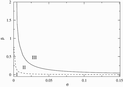
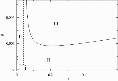
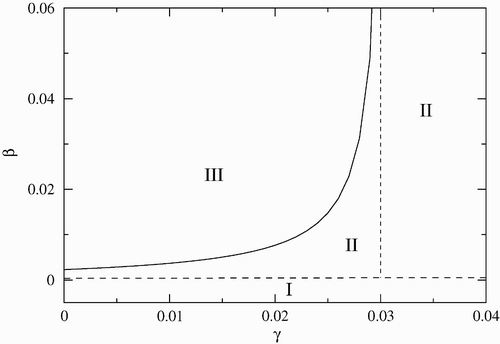
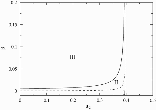
Most of the parameters are related to real data collected in the field and experiments. In all simulations μ _F , φ, C, and μ are kept fixed, and their values are μ _F =0.1, φ=0.4, C=200, and μ=0.0006, respectively. The other parameters have been varied to obtain the stability regions in the corresponding parameter space. We illustrate the different scenarios in several two-dimensional parameter spaces. In all figures, the solid line corresponds to the values of the parameters where Hopf bifurcation occurs, and the dashed line to the values where a bifurcation from the disease-free to endemic equilibrium takes place. Regions I, II, and III correspond to the stability regions of the disease-free equilibrium, the endemic equilibrium, and limit cycles, respectively.

Figure 1 illustrates the stability regions in the (β−σ) parameter space. In these simulations γ=0.01, μ _c =0, and α=0.07. The solid line corresponds to the critical values of β as a function of σ, where the dynamics of the endemic state goes through a Hopf bifurcation. We observe that above a minimum infection rate (β∼0.74) the disease cannot be eradicated, and the infected crab population either approaches the endemic equilibrium, or oscillates. The probability of periodic behaviour increases when the reproduction rate σ increases, and decreases as σ decreases. It is interesting to note that below a critical value of σ there are no limit cycles and solutions approach either the endemic or the disease-free equilibrium.

Figure 1. Stability region in the (β−σ) parameter space. Region I corresponds to the disease-free equilibrium, region II to the endemic equilibrium, and region III to limit cycles. The other parameters are fixed and given by γ=0.01, μ _c =0 and α=0.07.

In Figure 2 the stability regions are shown in the (β−α) parameter space with σ=1.4, γ, and μ _c as in Figure 1. Here, the Hopf bifurcation curve quickly decreases to a minimum for small values of the disease-induced mortality rate, α, and thereafter increases slowly as α increases. The minimum occurs at approximately α=0.1 and corresponds to the maximum-infected population size. Periodic solutions are not possible to the left of the dotted line α=0.04; the disease-free equilibrium is stable below the dashed line, and unstable above it, where the endemic equilibrium exists and is stable. Since α=τ⁻¹, where τ is the infectious period, large or small values of τ favors an endemic behaviour. Finally, it is interesting to observe that the minimum infection rate above which the infection cannot be eradicated is several orders of magnitude less than the corresponding one in Figure 1. This indicates that α is a determining factor for the establishment of the disease.

Figure 2. Stability region in the (β−α) parameter space. Region I corresponds to the disease-free equilibrium, region II to the endemic equilibrium, and region III to limit cycles. The other parameters are fixed and given by γ=0.01, σ=1.4 and μ _c =0.

The stability regions in the (β−γ) parameter space are given in Figure 3. The other parameters are the same as in previous figures. The solid line corresponds to the critical values of β as a function of γ where a Hopf bifurcation occurs. As in the previous case, the disease-free equilibrium region is very small. For values of γ to the right of the dotted line (γ>0.03), periodic solutions are not possible, and solutions approach the endemic equilibrium or the disease-free equilibrium, although the probability of the second case is very small.

Figure 3. Stability region in the (β−γ) parameter space. Region I corresponds to the disease-free equilibrium, region II to the endemic equilibrium, and region III to limit cycles. The other parameters are fixed and given by σ=1.4, μ _c =0 and α=0.07.

Finally, the bifurcation diagram in terms of (β−μ _c ) is illustrated in Figure 4. The values of the other parameters are as in the previous figures. In this scenario, the threshold curves that separate the stability regions are asymptotic to the line μ _c =0.4. To the right of this line R _C <1 implying that both populations go to extinction. We note, that as μ _c increases, the stability region of the endemic equilibrium increases.

Figure 4. Stability region in the (β−μ _c ) parameter space. Region I corresponds to the disease-free equilibrium, region II to the endemic equilibrium, and region III to limit cycles. The other parameters are fixed and given by γ=0.01, σ=1.4 and α=0.07.

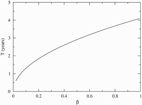
Figure 5 shows the frequency of the disease bursts as a function of the infection rate β. The Hopf bifurcation appears for β>0.012. As β increases, the time period between successive disease burst increases. Due to the great mortality of the infectious individuals, high infection rates drive the susceptible population to small values, and the disease dies out for large periods of time. Therefore, we can expect that in mangroves where the crab mortality due to LCD is high, the disease will take more time to appear again.

Figure 5. Period of disease oscillation as a function of β. The other parameters are μ _F =0.1, φ=0.15, γ=0.01, C=200, μ=0.0006, σ=0.7, μ _c =0.1 and α=0.07. The Hopf bifurcation appears for β>0.012.

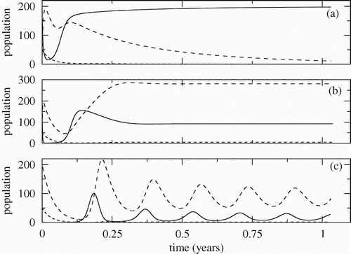
In Figure 6 we show the time evolution of the populations for three different infection rates β. Here, σ=0.25, and the other parameters are as in Figure 1. The continuous, dashed and dotted lines are susceptible crabs, infected crabs and fungus population, respectively. In (a) with β=0.02 (R _F <1) the populations approach the disease-free equilibrium ; in (b) with β=0.05 (R _F >1) the populations approach the endemic equilibrium; in (c) with β=0.29 (R _F >1) the populations have periodic behaviour. In all simulations we have R _C >1, so the trivial equilibrium is unstable. Of course, for this parameter set, in case (a), the fungus population goes to extinction, in (b) it goes to a small value different from zero and in (c) it oscillates around a small value.

Figure 6. Time evolution of the crab and fungus populations for the stability regions shown in Figure 1. The continuous, dashed and dotted lines are, respectively, the population of susceptible crabs, infected crabs and fungus. (a) Region I: convergence to disease-free equilibrium (β=0.02, R _F =0.87). (b) Region II: convergence to endemic equilibrium (β=0.05, R _F =2.17). (c) Region III: convergence to a limit cycle (β=0.29, R _F =12.57).

5. Conclusions

The present study represents the first attempt to model LCD, an infectious disease that has decimated populations of the mangrove land crab throughout the Brazilian coast. Little has been uncovered about LCD to date, despite the severity of the disease and the ecological and economic importance of its host. For this reason, it is imperative not only to learn the biological aspects of the disease but also to develop mathematical models to investigate its temporal and spatial dynamics. The use of theoretical models can address the relevance of intrinsic and extrinsic biological factors on the transmission of the disease, and can also be useful to investigate different scenarios about its control. The model formulated in the present study captures the essential features of LCD; in particular, it reproduces the periodic behaviour of LCD observed in several localities of Northeastern Brazil. The results are given in terms of the basic offspring of the crab, R _C , and the fungus population, R _F , as well as the transmission rate β.

The model has three equilibrium points. One corresponds to the absence of the two populations, and the system evolves to this state when R _C ≤1 (see Theorem A.1). In nature, this equilibrium is not feasible because there is larval exchange between the estuaries that would supply new individuals in each generation. For R _C >1, and R _F ≤1 solutions approach the disease-free equilibrium and the disease can be controlled in this case. R _F is proportional to the reproductive rate of fungus σ, which is a measure of the virulence of the pathogen, and to the infectious rate β, which is a measure of the crab susceptibility to infection. Conversely, R _F is inversely proportional to the fungus’s mortality rate, μ _F , i.e. proportional to its lifespan. Therefore, the infection can be controlled, combating fungus population in nature, and/or decreasing the crab susceptibility to the pathogen. A brief reflection indicates that the first alternative is undesirable, since a substance that destroy the fungus of LCD probably would affect other fungus which are essential for the balance of the mangrove ecosystem. Thus, the only viable control is to decrease crab susceptibility to the pathogen by the introduction of resistant crabs to the affected areas. Efforts in this direction has been done in Brazil. In particular, research to produce genetically resistant crabs cultivated in laboratories is developing 18.

The model also predicts that moderate crab capture decreases R _F and, depending on the value of the parameter β, can decrease the probability of disease bursts or increase the probability of the disease becoming endemic. In the first case, capture reduces the susceptible population below the threshold value needed to maintain the disease. In the second case, although the disease is maintained, the number of susceptible is not sufficiently high to produce periodic epidemic peaks. In both cases, the crab population is very close to extinction. We consider that it is necessary to conduct more studies to understand the influence of the crab capture on the disease dynamics.

When R _F >1, the endemic equilibrium where the disease persists all the time emerges. For suitable sets of the eight parameters, a Hopf bifurcation occurs, and then the disease dynamics can evolve to an endemic situation or can have an oscillatory behaviour. Therefore, the model results suggest that oscillations are produced by the interplay of constant demographic and epidemiological parameters, contrary to the hypothesis that such oscillations are a consequence of external forcing such as the stress associated with the mating season.

In this work, we chose the infection rate, β, as the bifurcation parameter. We found conditions (Equation (14)) as well as the neutral surface (Equation (15)) where the endemic equilibrium goes through a Hopf bifurcation. Using numerical simulations, we obtained the stability regions of the equilibria and limit cycles for two-dimensional parameter space while the other parameters remain fixed.

The numerical simulations given in section 4 show that increments of the infection rate β, and/or fungus reproduction rate σ increase the probability of oscillations as well as their period (see Figures 1, 5 and 6). Thus, in areas where crabs are more susceptible, or fungus is more virulent, the occurrence of periodic events with great epidemic peaks is higher. In both cases, cycles occur because the susceptible population almost disappears after an epidemic episode, and thereafter the fungus population decreases. When the susceptible population recovers to a threshold, another epidemic peak occurs, and so on. Conversely, Figure 3 relates increasing recovery rate γ to an endemic situation. In this case, the model behaves as an SIS model in which there is always a critical number of susceptibles to maintain the disease, due to the recovery of infected ones.

It is interesting to note that decreasing the disease mortality rate α below a threshold, or increasing it, promotes endemic behaviour (see Figure 2). Then, the model conjectures that LCD gradually becomes endemic in the regions where the disease induces a great mortality.

The lack of genetic structure among crab populations in the Brazilian coast 14 15 reflects the fact that crab larvae are capable of using ocean currents to disperse for dozens of kilometres from their native estuaries 3 16, promoting colonization of new estuaries. On the other hand, since fungus that causes LCD is resistant to ocean salinity, it is possible that its transmission to other estuaries is due to dispersion. Some numerical simulations have shown that, for small values of the migration rate, the model dynamics do not change qualitatively. Nevertheless, more studies are needed to understand the interplay between migration and infection. For this reason, we have in mind for the future to address this problem.

Acknowledgements

LE acknowledges a grant from PAPIIT IN08607–UNAM and CPF acknowledges a grant from FAPESP 05265-1/2007 and CNPq 478544/2007-3. MRP, WAB, and AO were partially funded by Companhia de Desenvolvimento Industrial e de Recursos Minerais de Sergipe (CODISE) and BahiaPesca, Brazil. PFAM acknowledges grants from FUNDUNESP 00238/08-DFP and CAPESP Pró-equipamentos 01/2007. We are also grateful to two anonymous referees for their valuable comments that helped to improve this paper.

Appendix 1. Stability of the trivial equilibrium E ₀

Theorem A.1

If R _C ≤1, then all solutions of system (1) in approach the trivial equilibrium E ₀ .

Proof

Consider the Lyapunov function with Lyapunov derivative given by

The last inequality holds because R _C =φ/a≤1. The Lyapunov-Lasalle Theorem 8 implies that all solutions in approach the largest positively invariant subset of . It is clear that when S=I=0. Then in M system (1) becomes S′=0, I′=0, F′=−μ _F F, which implies that as . Thus, E ₀ is the only positively invariant subset of M. Hence, all solutions in approach that point.   ▪

Appendix 2. Stability of the disease-free equilibrium E ₁

Theorem B.1

Assume R _C >1. If then all solutions of Equation (1) in Ω={(S, I, F)|S>0, I≥0, F≥0} approach the disease-free equilibrium E ₁ .

Proof

Consider the Lyapunov function defined in Ω,

It can be seen that (see 6) and its Lyapunov derivative is given by

Substituting from Equation (2), and simplifying gives

for . It is clear that if and only if , I=0, and F=0. Again, for the Lyapunov-Lasalle Theorem 8 this implies that all trajectories in Ω approach E ₁ as .   ▪

For R _F <1 and γ sufficiently small, . Therefore, the result above shows that the LCD can be effectively controlled if the basic reproductive number of the fungus, R _F , is less than one, and the recovery rate of the infected crabs is nearly zero.

References

- Aron , J. L. and May , R. M. 1982 . “ The population dynamics of malaria ” . In Population Dynamics of Infectious Diseases , Edited by: Anderson , R. M. London : Chapman and Hall .
- Boeger , W. A. , Pie , M. R. , Ostrensky , A. and Patella , L. 2005 . Lethargic crab disease: multidisciplinary evidence supports a mycotic etiology . Mem. Inst. Oswaldo Cruz , 100 ( 2 ) : 161 – 167 .
- Boeger , W. A. , Pie , M. R. , Vicente , V. A. , Ostrensky , A. , Hungria , D. B. and Castilho , G. G. 2007 . Histopathology of the mangrove land crab Ucides cordatus (Ocypodidae) affected by lethargic crab disease . Dis. Aquat. Organ. , 78 : 73 – 81 .
- Diele , K. and Simith , D. J.B. 2006 . Salinity tolerance of northern Brazilian mangrove crab larvae, Ucides cordatus (Ocypodidae): necessity for larval export? . Estuarine Coast. Shelf Sci. , 68 : 606 – 608 .
- Diele , K. , Koch , V. and Saint-Paul , U. 2005 . Population structure and catch composition of the exploited mangrove crab Ucides cordatus in the Caet estuary, North Brazil: Indications of overfishing? . Aquat. Living Resources , 18 : 169 – 178 .
- Glaser , M. 2005 . Interrelations between mangrove ecosystem, local economy and social sustainability in Caeté Estuary, North Brazil . Wetlands Ecol. Manage. , 11 : 265 – 272 .
- Goh , B. S. 1977 . Global Stability in Many Species Systems . Am. Nat. , 111 ( 997 ) : 135 – 143 .
- Guckenheimer , J. and Holmes , P. 1993 . “ Nonlinear Oscillations, Dynamical Systems, and Bifurcations of Vector Fields ” . In Applied Mathematical Sciences , Vol. 42 , New-York, Berlin, Heidelberg : Springer-Verlag .
- Hale , J. K. 1981 . Ordinary Linear Equations , New York : Wiley-Interscience .
- Heffernan , J. F. , Smith , R. J. and Wahl , L. M. 2005 . Perspectives on the Basic Reproductive Ratio . J. R. Soc. Interface , 2 ( 4 ) : 281 – 293 .
- Legat , J. F.A. , Mota , R. I. , Puchnick , A. , Bittencourt , C. and Santana , W. S. 2006 . Considerations about Ucides cordatus cordatus fishing in the Parnaiba River Delta region, Brazil . J. Coast. Res. , 3 : 1281 – 1283 .
- Melo , G. A.S. 1996 . “ Manual de identificação dos Brachyura (caranguejos e siris) do litoral brasileiro ” . 604 São Paulo, Plêiade/FAPESP .
- Mena-Lorca , J. and Hethcote , H. W. 1992 . Dynamic Models of infectious diseases as regulators of population sizes . J. Math. Biol. , 30 : 693 – 716 .
- Nordhaus , I. and Wolff , M. 2007 . Feeding ecology of the mangrove crab Ucides cordatus (Ocypodidae): food choice, food quality and assimilation efficiency . Mar. Biol. , 151 : 1665 – 1681 .
- Nordhaus , I. , Wolff , M. and Diele , K. 2006 . Litter processing and population food intake of the mangrove crab Ucides cordatus in a high intertidal forest in northern Brazil . Estuarine Coast. Shelf Sci. , 67 : 239 – 250 .
- Oliveira-Neto , J. F. , Pie , M. R. , Boeger , W. A. , Ostrensky , A. and Baggio , R. A. 2007 . Population genetics and evolutionary demography of Ucides cordatus (Decapoda : Ocypodidae) . Mar. Ecol. , 28 : 460 – 469 .
- Oliveira-Neto , J. F. , Boeger , W. A. , Pie , M. R. , Ostrensky , A. and Hungria , D. B. 2007 . Genetic structure of populations of the mangrove crab Ucides cordatus (Decapoda : Ocypodidae) at local and regional scales . Hydrobiologia , 78 : 73 – 81 .
- Schwamborn , R. , Ekau , W. , Silva , A. P. , Silva , T. A. and Saint-Paul , U. 1999 . The contribution of estuarine decapod larvae to marine zooplankton communities in North-East Brazil . Arch. Fishery Mar. Res. , 47 : 167 – 182 .
- Swart , J. H. 1989 . Hopf bifurcation and stable limit cycle behaviour in the spread of infectious disease, with special application to fox rabies . Math. Biosci. , 95 : 199 – 207 .
- Wolff , M. , Koch , V. and Isaac , V. 2000 . A trophic flow model of the Caete Mangrove Estuary (North Brazil) with considerations for the sustainable use of its resources . Estuarine Coast. Shelf Sci. , 50 : 789 – 803 .
- Revista do Gia (Grupo Integrado de Aqüicultura e Estudos Ambientais), Desvendando uma tragédia nos manguezais brasileiros 2 (49) (2006)
- Zhou , J. and Hethcote , H. W. 1994 . Population size dependent incidence in models for disease without immunity . J. Math. Biol. , 32 : 809 – 834 .