A mathematical model of the population dynamics of disease-transmitting vectors with spatial consideration

Abstract

A deterministic model with spatial consideration for a class of human disease-transmitting vectors is presented and analysed. The model takes the form of a nonlinear system of delayed ordinary differential equations in a compartmental framework. Using the model, existence conditions of a non-trivial steady-state vector population are obtained when more than one breeding site and human habitat site are available. Model analysis confirms the existence of a non-trivial steady state, uniquely determined by a threshold parameter, , whose value depends on the distribution and distance of breeding site j to human habitats. Results are based on the existence of a globally and asymptotically stable non-trivial steady-state human population. The explicit form of the Hopf bifurcation, initially reported by Ngwa [On the population dynamics of the malaria vector, Bull. Math. Biol. 68 (2006), pp. 2161–2189], is also obtained and used to show that the vector population oscillates with time. The modelling exercise points to the possibility of spatial–temporal patterns and oscillatory behaviour without external seasonal forcing.

Keywords:

• vector-breeding sites and human habitat
• Hopf bifurcation
• flight range domain
• population dynamics
• compartmental framework

2000 AMS Subject Classification :

• 34A
• 34C
• 92B

1. Introduction

Vector-borne diseases (e.g. malaria, dengue, fever, yellow fever, lyme disease, trypanosomiases, and leishmania), amongst all the human infectious diseases, continue to remain a public health concern and a severe burden on economies, causing high human mortality in the world. These diseases have not only posed problems to national economies, but have also caused poverty and low living standards, especially in countries in the tropical and subtropical regions of the worlds. For example, the vector-borne disease, malaria, caused by the plasmodium parasite and transmitted from one human to another by the female anopheles vector mosquito, continues to plague the world especially the developing nations. By the WHO World malaria report 22, the parasite, and hence malaria, caused an average of nearly 900,000 thousand deaths in 2006, of which 85% were of children under the age of five. Also, dengue fever, yellow fever, trypanosomiases, and leishmania are all highly prevalent tropical and subtropical diseases. Some vector-borne diseases, such as malaria, dengue, and yellow fever, that used to be common in some developed nations of the world have been successfully put under control 3. However, these diseases are still a threat to developing nations and hence a potential threat to many regions of the world. Given recent trends in climate change 2, global warming 6 7, and increased movement between different nations, disease-transmitting vectors may be able to (re)-colonize and survive in zones not formerly possible. Therefore, understanding the population dynamics of vectors that transmit diseases is an important area of scientific inquiry.

The main agents necessary for a successful transmission of a vector-borne disease are: the transmitting vector,1 the infectious agent,2 and the host.3 For the success of these diseases, the infectious agents adapt their life cycle so that part of it is harboured in the host and the other part in the vector, with the vector being the vehicle that transports the disease agent from one host to another. Hence, it is essential to study and understand the mechanism by which these transmitting vectors operate from a mathematical modelling perspective. Here, our focus will be on these vectors, with the main objective being to understand the dynamics of the transmitting vehicles – the vectors, by taking into consideration their behavioural aspects, their interaction with hosts, and their breeding patterns and habitats. Our special interest will be on insect-transmitting vectors though the ideas can easily be applied to any blood-sucking vector.

The geographical and local distribution of different kinds of disease-transmitting vectors in different regions is determined by a complex set of factors – climatic and geographic factors, or may even be associated with hosts endangered by the vectors 15. However, the basic transmission pattern for most vector-borne diseases are similar. The vectors interact with the host in some way, for the most part, in search of blood or other factors that can enhance its successful existence over different generations. During this interaction and search, the vector may either be successful or may fail and seek to try again, or may be killed. Upon a successful interaction, the vector may be infected by an infectious agent or on the other hand infect the host with an infectious agent. In our analysis, we will consider that a vector actively seeks the host 8 and hence seeks the interaction with a host. In addition, the vector lives, rests, and breeds in a habitat (vector-breeding site) and the host also lives and reproduces in its habitat with both habitats interacting. In trying to model the disease-transmitting vectors, we will focus on blood-feeding vectors with distinct stages of development, which include an egg laying, larval development, and adult eclosion vector stage, harboured in different breeding sites and habitats. In our modelling, these metamorphic stages of development will be accounted for. In addition, the model will take into consideration the human populations in their habitats that are endangered by the disease-transmitting vectors (not necessarily the disease) and the interactions between the two habitats.

Mathematical models to study such vector dynamics and in particular mosquito dynamics have been rare. Most models have focused on the population dynamics of disease agents, e.g. in the case of malaria see 11 13 14 17 19, or on the dynamics of the disease agent within a host 9 or within a vector 18 20. Ngwa 12 introduced a deterministic delayed differential equation model of the population dynamics of the malaria vector when only a single host habitat and single vector (mosquito) habitat or breeding site is concerned. His model incorporated vector deaths in stages prior to the adult vector eclosion stage. With his model, he showed that when a non-zero steady-state vector population density exists, it can be stable but can also be driven to instability via a Hopf bifurcation to periodic solutions.

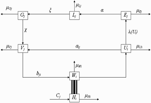
Here, we extend the deterministic model by Ngwa 12, to include more than one vector-breeding site and also more than one host habitat. The goal will be to understand how variation in the number of human habitats or variation in the number of breeding sites enhances or affects the interaction between the vector habitat or breeding sites and the host habitat dynamics and how this ultimately affects the dynamics and existence of the vector populations. Secondly, the solutions derived from the mathematical model will be obtained and studied to ascertain that oscillatory dynamics known to exist within disease vector populations are captured. The compartmental framework on which we base our model is displayed in Figure 1.

Figure 1. Schematic framework showing the inter-relationship between the different classes of vector populations and also the life cycle of vectors at breeding site.

The rest of the paper is organized as follows: In Section 2, we define the notations used, describe the methodology used, outline the essential assumptions, and briefly derive the mathematical model. In Section 3, the analysis of the interactive model is presented. In addition, we analyse the existence and stability of the steady-state vector and host population densities. In Section 4, we simplify our model for the vector population densities by studying a simple case (one-human habitat–one-vector-breeding site). For this simple case, we establish the stability of the non-zero steady state with help of Hopf bifurcation methods. We round up with a conclusion and discussion in Section 5.

2. Derivation of the model

The basic model divides the entire vector population into three compartmental classes representing physiological status. These classes are: the class of fed and reproducing vectors returning from human habitats to vector-breeding sites represented by the variable U; the class of unfed and resting vectors present at vector-breeding sites represented by the variable V; and the class of unfed vectors questing (or foraging) for food (blood meal) in human habitats represented by the variable W. Each class of vectors is again subdivided into subclasses representing spatial locations. If we assume that there are M human habitats , and N vector-breeding sites , then the classes of vectors U, V, and W are subdivided into subclasses U _i , V _j , and W _i , i=1, …, M, j=1, …, N, respectively, where U _i ’s represent fed vectors returning from location , W _i ’s represent unfed vectors foraging for food at location , and V _j ’s are unfed and resting vectors resting at the vector-breeding site . With these considerations, at time t we have

If N _v (t) is the total density of vectors at time t, then we have

The human population, on the other hand, is divided into classes representing spatial locations. This means that if the density of the entire human population at time t is H(t), then H(t) is divided into classes H _i (t), i=1, …, M, where each H _i (t) represents the density of humans present at location at time t, ∀ i. We also have

For the analysis, it is assumed that vectors of type V _j are located at breeding sites , j=1, …, N, in which they grow by undergoing four stages of metamorphosis (). They experience natural death at rate . In the interactive model, we take into consideration only adult female vectors. Thus, all vectors present at the breeding site are either young emerging adult vectors or vectors that have just returned from the human habitat. Also, vectors located at , can make visits to the human habitat , in search of a blood meal. When a vector leaves the breeding site and arrives at human habitat (to forage for blood meal), it immediately becomes a vector of type W _i , and the decision by such a vector to visit a particular human habitat, , is influenced by how far the human habitat is from the vector-breeding site, as well as the number of resource agents (humans) present at the human habitat. At habitat , vectors W _i interact with human according to standard mass action principle with a contact rate τ _i . This interaction is successful with probability p∈[0, 1] and a blood meal is taken, or else, it is unsuccessful with probability (1−p) and the vector is assumed killed. Vectors of type W _i experience natural death with rate denoted by . It is assumed that all vector-breeding sites are equally safe and that there is a constant alternative blood source for the vectors (may be from animals). However, we assume that the anthropophilic4 vectors, which form the basis of our mathematical study, have such a strong preference for human blood that they would fail to live in the absence of humans. Vectors which have successfully obtained a blood meal at human habitat join the class U _i of fed vectors returning to breeding site , . We assume that the decision by such a vector to go to a particular breeding site depends on how far the breeding site is from the human habitat, and perhaps on the degree of safety and availability of other vectors at that site. Vectors of type U _i experience a natural death at rate . In this paper, we do not take into consideration intervisitation of breeding sites by vectors.

Next, humans reside at human habitat , i=1, …, M, and for each i, the human population density at time t is labelled H _i (t). We assume that there is a net constant migration, C _i , of humans in habitat and that the humans experience a per capita natural death rate . The term C _i incorporates births, immigration, and emigration. Humans from habitat migrate to other human habitat at rate . In human habitat , the humans are visited by vectors and there is an interaction between the two species based on standard mass action contact. It is assumed at this stage that the humans do not suffer any deaths that can be directly associated with their contact and interaction with the vectors.5 However, every vector that interacts with a human and fails to obtain a blood meal is assumed killed. For a two-dimensional consideration, let d ₂: be the usual metric on ℝ². In other words,

Then, d ₂ is the standard Euclidean distance between the points and in ℝ². We then define the closed ball centred at of radius d, denoted by

This closed ball is a disc with radius d and centre in Euclidean ℝ². Define

and

Then, A _ij and B _ij are smallest when is ‘far’ from zero and largest when is ‘near’ zero. A _ij and B _ij may be regarded as flow rates from breeding site to human habitat and from human habitat to breeding site , respectively. It is evident that both forms for A _ij and B _ij suit our assumption that more vectors flow from breeding sites to nearest human habitats and vice versa. Additionally, in our definitions for A _ij and B _ij , the radius d will represent the maximum flight range of vectors.

It can be shown 12 that the net rate of adult eclosion at breeding site j resulting from vectors coming from human habitat sites i, for i=1, …, M, is

where , and T _g represent, respectively, the maturation times of the vector in previous life stages, is a birth rate function for vectors at breeding site , μ_e, μ_l, and μ_g are, respectively, the natural death rates for egg, larva, and pupa, the earlier life stages of the vector. Formula (7) represents the progeny of some fed vectors, U _i (t), which returned from human habitat to the breeding site and laid eggs units of time ago. Each of the exponential expressions , , and represent the probability of survival at a particular developmental stage (respectively, egg, larva, and pupa). Therefore, if we take into consideration the progeny of fed vectors from all human habitats that are within the flight range of vectors at the particular breeding site , we have the total sum

For simplicity, we assume that and set , with all parameters positive.

2.1. Dynamics of human population

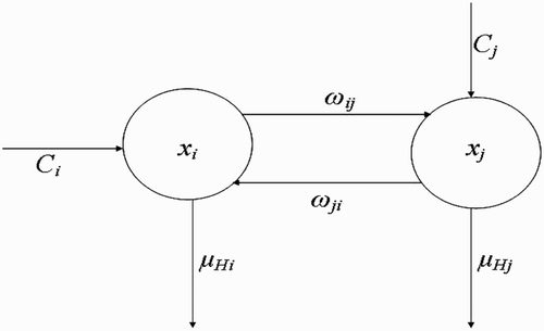
Let the density of human population at habitat be H _i (t). Let also C _i incorporate births, emigration, and immigration. Suppose that these resource agents, H _i , experience a constant natural death rate and migrate to human habitat at rate w _ij (see the flow diagram in Figure 2 which describes this situation). Then, the rate of change of H _i (t) with respect to time t could be written as follows:

where C _i , w _ij , and are positive constants, .

Figure 2. Dynamic interplay or migration between humans at habitat x _i and humans at habitat x _j .

2.2. Dynamics of vector population with spatial characteristics

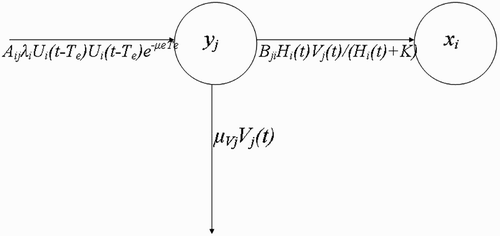
Vectors at the breeding site (V _j ): From Equation (8) and the assumptions and , we have that

is the total progeny at breeding site of vectors U _i that returned from all human habitats , that are within the flight range of vectors at breeding site , with T being the time lapse between egg-laying and adult vector eclosion. We assume that a fraction

of vectors prefer human blood meal. Here, α _v is the anthropophilic factor,6 while β _v is the zoophilic factor7 of vectors. In addition, let us take A _ij and B _ij to be the respective flow rates of vectors from breeding site to some human habitat and that of vectors from human habitat to some breeding site as defined in Equations (5) and (6), respectively. Also, let these vectors at the breeding site die naturally at a constant rate . Then using the flow diagram in Figure 3, showing the dynamic interplay between vectors at breeding site and human habitat , the rate of change of V _j (t) with respect to time t may be written as

where the sum is taken over all human habitat sites that communicate with the vector-breeding site, . Here, we assume that a human habitat site and a vector-breeding site communicate with each other if both sites are within the flight range, d, of the vector.

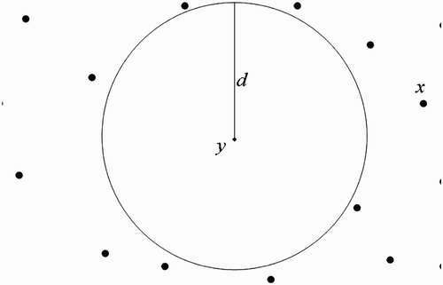
Figure 3. Schematic framework that models the flow of vectors V _j (t) from breeding site y _j to human habitat x _i .

Vectors visiting resource agents (questing vectors) (W _i ): Vectors from a particular breeding site, , are attracted to human habitat, (see the flow diagram in Figure 4), at the rate

and return to breeding site with rate A _ij , which is determined solely by proximity (we have chosen not to include whether the presence of vectors at a breeding site may aid returning vectors in choosing that breeding site because we are not aware of any strong scientific evidence that supports these claims). We consider that these questing vectors interact with humans in human habitats according to the principle of mass action, with contact rate , and that they succeed with probability p∈[0, 1] and fail with probability (1−p), in which case they are assumed killed. We further consider that the questing vectors experience a constant natural death rate . Figure 4 displays a flow diagram that shows the changes occurring in the vectors after interacting with the humans.

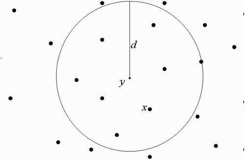
Figure 4. Changes in the population density of questing vectors W _i with respect to time t, resulting from their interaction with humans at the human habitat x _i .

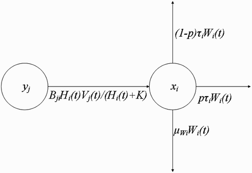
Then at the human habitat , i=1, …, M, the rate of change of the population density of the questing vectors with respect to time is

where , , i=1, …, M, are positive constants and the sum is taken over all vector-breeding sites that communicate with human habitat site .

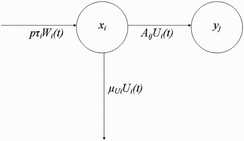
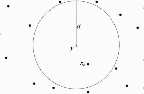
Vectors returning from resource agent sites (U _i ): Let U _i be the vectors which succeed in their quest for blood at the human habitat . They can move to any of the breeding sites , j=1, …, N, within their flight range, at rate A _ij . Suppose also that the fed vectors experience a natural constant death rate as they return to the breeding sites. Then using the flow diagram (Figure 5), the rate of change of U _i (t) with respect to time t can be written as

where , i=1, …, M, j=1, …, N, are positive constants and the sum is taken over all breeding vector sites which communicate with the human habitat site .

Figure 5. Dynamic interplay between fed vectors U _i at human habitat x _i returning to breeding site y _j .

Next, we make the following assumption.

Assumption 2.1

for all integers k and l not belonging to the sets and , respectively, .

Then without loss of generality, setting

and assembling Equations (9)–(12) together with Assumption 2.1, we obtain the following system of 3M+N equations in the 3M+N variables H _i , U _i , W _i , and .

Notice that the equation for H _i (t) decouples from the rest of the system.

To complete the formulation, it is expedient to give an explicit functional form to the function λ: and also to supply the initial data for our model. We begin with the functional form.

Definition 2.1

A function is a suitable birth rate function for the vectors of type U if it satisfies the following three assumptions:

• A1: 

• A2: λ(U) is continuously differentiable with

• A3: There exists a positive number, called the vectorial basic reproduction number (denoted by such that

Assumptions A1 and A2 ensure the existence of for x>0, with , while Assumption A3 ensures the existence of a threshold parameter, ℛ₀, with the property that, when , a positive non-trivial equilibrium, given by

exists. This equilibrium does not exist if .

The choice of the functional form of λ(U) is based on the fact that in ecology nonlinearity in the dynamics of the population of a single species can arise due to competition, usually for resources, between members of the population. When there is competition for a common resource between members of the same species, two types of competition can be identified, namely contest competition (competition for a resource that is partitioned unequally so that some competitors obtain all they need and others less than they need (i.e. there are winners and losers)) and scramble competition (competition for a resource that is inadequate for the needs of all, but is partitioned equally among contestants, so no competitor obtains the amount it needs) 5. It seems reasonable to assume a contest type competition for mosquito dynamics based on the fact that there is abundance of humans for blood meal; however, some of the vectors are killed (losers) in their quest for a blood meal. In this paper, the following form of birth rate function, which satisfies Assumptions A1–A3, will be used:

where and L _i >0 are positive constants. To ensure that Assumption A1 is satisfied, L _i is assumed very large and may be identified as the carrying capacity of environment created by habitat , while may be regarded as the limiting rate at which vectors from human habitat would lay eggs if the population of the vectors should become very small. This functional form, commonly known as the Verhulst–Pearl logistic growth model, has been used in previous studies 12. Other nonlinear birth rate functions can be used. For example: the Beverton–Holt function or the exponential or modified form of the Skellam function , or the Maynard–Smith–Slatkin function for some positive n). See 1 for more on these functional forms. The main reason for using the Verhulst–Pearl function is because of its linearity. In fact, it is a general form for a first linear approximation to any nonlinear form of birth rate function satisfying Assumptions A1–A3. The mathematical assessment of the role of nonlinear birth in the population dynamics of disease-transmitting vectors is under investigation.

Next we define initial data for t∈[−T, 0] as follows:

where , and u _i (t) are some continuously differentiable functions. Thus, the equations governing the rate of change of the total human and vector population densities, simply obtained by adding up the relevant equations from above (as given by Equations (2) and (3)), are

with appropriate initial conditions,

We observe that in the present formulation, the equation governing the human population, though influencing the size of the vector population, is decoupled from the system in the sense that those equations can be analysed separately. It is also clear from Equations (13) and (14) and the above formulation that if , then as , since then . We take up the analysis of the interactive model in the next section.

3. Analysis of the interactive model

In this section, we examine the spatially explicit model and show that there exists a steady-state spatial distribution of vector populations over the entire region of study (N>0, M>0 arbitrary) and derive conditions under which such population densities could exist. Before this, we briefly analyse the dynamics of the human population.

3.1. Existence of a steady-state human population density

Here, we examine the existence and stability of steady-state solutions for the density of human populations. In this section, we shall assume that the death rate of humans, , are identical for all habitats. In addition, we assume that the migration of humans between any two human habitats, w _ij , is also identical so that and w _ij =w, where w and μ are constants. This means that the human habitats are identical. To examine and analyse the stability of the steady state of the human population, we state and prove a lemma and theorem that will be essential.

Lemma 3.1

Let be an n×n real symmetric matrix depending on positive parameters x, y. If in addition, for each the matrix has only two distinct elements such that

then for has only two distinct eigenvalues. Furthermore, all the eigenvalues of the matrix are real and negative and satisfy

where is the identity matrix of size n×n.

Proof

Let n≥2 be an integer. We easily verify that

where is the n×n matrix

Then, direct computation by cofactor expansion shows that at the kth stage of the expansion, for k≤n, for any n≥2, we have the relation

Now,

Hence,

This therefore gives us

  ▪

We now use Lemma 3.1 to prove the following theorem.

Theorem 3.2

The linear system of equations

with (w and μ are constants), for any values of C _i , has a unique non-zero steady-state distribution of humans over the M habitat sites whose value for each i, is given by

Moreover, the postulated steady state is globally and asymptotically stable.

Proof

We examine Equation (20) when the time derivatives are set to zero. Let be the steady-state solution. Then on setting w _ij =w and , as assumed, we obtain that satisfies the system

If we let

and then substitute in Equation (22), we obtain

which when we substitute into Equation (23), and then solve for H*, results to

We next substitute Equation (25) into Equation (24) to obtain Equation (21). To establish the stability of this steady state, let

If we substitute Equation (26) into Equation (20) with , for all i, j, we obtain the analogous linear system

If we seek solutions of the form , where ξ is an eigenvalue that measures the temporal growth of the solution at time t, this leads to the solvability condition

where is the identity matrix of size M and is the M×M matrix with every off-diagonal elements being w and all diagonal elements being −μ−(M−1)w. That is,

Hence from Lemma 3.1, we obtain that

Thus, the eigenvalues are all real and negative, and the steady-state solution is globally and asymptotically stable for all values of the parameters.

Remark 3.1

The extension of the results of Theorem 3.2 to cover the general cases, where are different, is solved by observing that Equation (20) can be written in matrix form as

where the matrix is defined as

from which the steady states can be easily obtained and the system analysed based on the properties of . However, for our analysis, we will consider the simpler case where the human habitats are assumed identical since we are using human habitat here to refer to a location in space where there are humans from whom mosquitoes can quest for blood. The real structure and property of that spatial location does not really make a difference, since the differentiating feature is the presence of humans which has been captured by the model.  ▪

3.2. Existence of a steady-state vector population density

We examine in this section the spatially explicit model for the distributions of vectors. We show that there exists a spatial distribution of vector population densities over the entire region of study and derive conditions under which such steady population densities could exist. Our focus is now on the following three equations (taken from system (14)):

The steady states are obtained by setting the time derivatives in Equations (33)–(35) to zero and solving for the 2M+N quantities , and We then establish that

Also, substituting Equation (36) into Equation (33) when the right-hand side is equated to zero gives

Equations (36) and (37) show that we can calculate the steady-state values, and , once the ’s are known. We see that when , we have and . If , then the dynamic interaction between the human and vector populations establishes a non-zero steady-state population of vectors of all categories in all the human and vector sites that are within the flight range of the vectors from the particular breeding site . For each j, referring to Equation (34) and using the postulated form (15) for λ _i , the ’s should satisfy the N equations

where

are positive constants. Now, using the form of given in Equation (37), we set

so that Equation (38) for the steady state then takes the form

Q _jkl (T) and S _jk (T) as defined above are all positive constants. We also note that and . This relation simply captures the symmetry in the problem under consideration which arises due to the fact that when a human habitat site is within a vector breeding site , then the two sites communicate. In Equation (44), all parameters are positive and the relation must hold for all values of j. We observe that , is a solution. That is, the trivial steady state is the same for sites which are within a communicable distance. But when , the result is a system of N nonlinear equations for which the description of the solutions is not apparent in view of all arbitrary values of the parameters. However, from a mathematical (and physical) perspective, all we wish to establish is whether there exists a non-negative solution, the steady-state solution, for the system (44).

Definition 3.1

Let S _v and S _h be the sets of all vector-breeding and human habitats sites, respectively, and . Let , d>0 the maximum flight range of vectors from location . Define

Then, we call the flight range domain of vectors from location x , where d ₂ is the metric defined in Section 2, with domain . We similarly define the flight range domain for

Definition 3.2

Let , ’s the flight range domains of vectors at ’s, i=1, …, r, respectively. We say that the ’s are disjoint if

Definition 3.3

Let ’s the flight range domains of vectors at ’s, i=1, …, r, respectively. We say that the ’s are one-point-intersected if

In this case,

Definition 3.4

• (i) Let . We define the distance from a site to the set A as

• (ii) Let , ’s the flight range domains of vectors at ’s respectively. We say that the ’s full-intersect if there exist at least two sites s.t.

  We set .

Definition 3.5

Let and i=1, …, r ₁, j=1, …, r ₂, Suppose and s.t. and Define

where ∂ A is the boundary of A, for any set A (Notice that and where and are singleton sets). We call U _h the unit of the human habitats , i=1, …, r ₁, and U _v the unit of the vector-breeding sites . We call the centre of U _h and the centre of U _v .

Remark 3.2

We similarly define the concepts of disjoint, one-point-intersection and full-intersection flight range domains when ’s, , are taken in S _h .

We state and prove the following proposition using the case study approach that is later generalized.

Proposition 3.1

The system (44) has exactly a two-solution set in which . The trivial solution, which always exist, and a non-trivial solution, with whose existence is uniquely determined by a threshold parameter ℛ in the sense that

• (a) if then the system has no positive non-zero real solutions;

• (b) if then the system has exactly one real positive non-zero solution.

Proof

In all the proofs, we suppose that , since the solution is trivial. Without loss of generality, we rewrite Equation (44) replacing by V _j , ∀ j:

Case 1: N=1

(a) We first consider the situation where human habitats are not found within flight range domain of vectors at breeding site (Figure 6).

Figure 6. Diagram showing various human habitats not belonging to flight range domain R _y .

In this case, we deduce from (5), (6), and (13) that

This implies that

so that Equation (45) is simply

The solution of Equation (46) is the trivial steady state

which is what we expected, since an assumption made during the derivation of our model was that the vectors do not survive in the absence of human population. Therefore, if vectors cannot interact with humans at human habitats, then their population will die out.

Assumption 3.1

Within their flight range domain, vectors located at breeding site always have a unit of human habitats, centred at where they find blood meal to live and prosper.

(b) We now suppose that human habitats belong to the flight range domain of vectors located in breeding site (Figure 7).

Figure 7. Diagram showing various human habitats belonging to flight range domain R _y .

Taking into consideration Assumption 3.1 and using Figure 8, we shall use the centre of the unit U _y to represent all the human habitats within the flight range of vectors located at (we therefore think as if we have a system with one breeding site and one human habitat found within the flight range of vectors located at the breeding site), set

and substitute these into Equation (45) to have the equation

from which we derive the non-zero steady-state solution

In order that V>0, we should have

We therefore derive an expression for :

Case 2: N=2 In this case, Equation (45) becomes

Let and be the two breeding sites in the study. Let the centres of the units of each of the two breeding sites be, respectively, and .

• (a) Disjoint flight range domains (Figure 9):

  In this case, , therefore vectors in do not visit sites in , and vice versa. Then by Equation (13), we obtain

  Substituting Equation (51) into Equations (42) and (43), we get
  Substituting Equation (52) into Equation (50) gives
  which has as solution set when , the singleton
  We observe that for j=1, 2,
  This implies the following definition

• (b) One-point-intersection flight range domains (Figure 10):

  We consider here vectors present in human habitats , and intersection of the flight range domains and . At this site , vectors decide (according to our assumptions), after a successful interaction with humans, to return either to the breeding site , or to the breeding site , with equal chance. In Equation (13) where we define the rates at which vectors move from human habitat to vector-breeding site , and from breeding site to human habitat , respectively, we see that a _ij and b _ji depend essentially on the distance from to . With this, we obtain that at habitat x

  Substituting Equation (56) into Equations (39), (42), and (43), we have
  This means that at habitat x, all parameters are constant and positive (this is easily verified). Substitute Equation (57) into Equation (45) to obtain the following system of equations:
  Equate the two equations in Equation (58) to obtain
  Substitute this equality in any one of the equations in Equation (58) to have the following solution set
  For j=1, 2, we see that
  Therefore, we choose

• (c) Full-intersection flight range domains (Figure 11):

  Let , and and be the flight range domains of vectors present at and , respectively. Let us define the following:

Figure 8. Diagram showing centre of unit U _y as a representative of the whole unit.

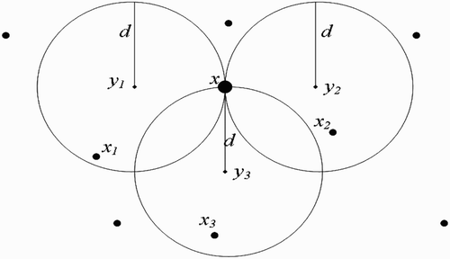
Figure 9. Disjoint flight range domains with the respective centres representing all the belonging human habitats.

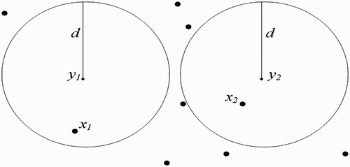
Figure 10. One-point-intersected flight range domains with the respective centres representing all the belonging human habitats.

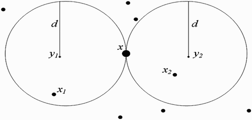
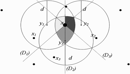
Figure 11. Full-intersected flight range domains with the respective centres representing all the belonging human habitats.

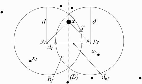
We make the following remark:

Remark 3.3

must belong to the line (D), which is equidistant to both and . For, if x does not belong to (D), then vectors present in x will choose to return to the nearest breeding site, that is or . Thus, cosθ cannot be equal to zero.

By considering the terms defined in Equation (61), we proceed as in the case of one-point-flight range domains above, with [dtilde] in the place of d, ã _ij and [btilde] _ji in places of a _ij and b _ji , respectively. We therefore obtain similar results, that is

and

where , and [Qtilde] are obtained by replacing a _ij and b _ji by ã _ij and [btilde] _ji , respectively, in Equations (39), (42), and (43).

Case 3: N=3 In this case, Equation (45) becomes

• (a) Disjoint flight range domains:

  For similar reasons as in previous cases,

  This implies that
  Equation (64) then becomes (using Equation (66))
  The non-zero solution of Equation (67) is the singleton set
  Again, for j=1, 2, 3,
  Therefore, we set

• (b) One-point-intersection flight range domains (Figure 12):

  this implies that
  Using Equation (71) into Equation (64), we obtain
  Equate all the equations in Equation (72) to have
  Substituting the last equality in any one of the equations in Equation (72), we have the following non-zero solution set
  From this, for j=1, 2, 3,
  Therefore, we define

• (c) Full-intersection flight range domains (Figure 13):

  We begin the following definition of a full point.

Figure 12. One-point-intersected flight range domains with three vector-breeding sites.

Figure 13. Full-intersected flight range domains with three vector-breeding sites.

Definition 3.6

Let j=3, …, N, be breeding sites. Let Δ _ij be the lines equidistant from and ∀ i, j. Then there are of these lines, with

Denote these lines by and define

We call F the full point, or simply the F-point, of the ’s.

We consider in the current situation only human habitat present at the F-point of , , and , for it is the only human habitat within flight range of vectors that is equidistant from all breeding sites.

As in Equation (61), we define the following:

and follow the same procedure as for the one-point-intersection case, with [dtilde] in the place of d, ã _ij and [btilde] _ji in places of a _ij and b _ji , respectively. We therefore obtained similar results. That is

and

where , and [Qtilde] M0080a _ij and b _ji by ã _ij and [btilde] _ji , respectively, in Equations (39), (42), and (43).

General case: N≥2

• (a) Disjoint flight range domains: As in previous cases,

  This implies that
  Using Equation (81) into Equation (45), we obtain the system of N equations
  which has as non-zero solution set the singleton
  This result tells us that within their respective flight range domains, vectors live and prosper whenever there is available nutrient from humans in human habitats. Observe that in the present situation, the number N of vector-breeding sites does not affect the value of the respective . From Equation (83),
  Therefore, we define

• (b) One-point-intersection flight range domains: As in previous cases, at the F-point,

  This implies that
  Using Equation (86) into Equation (45), we obtain the system of N equations
  Equating all equations in system (87), the following relation is clear:
  We use this equality into any one of the equations of the system and obtain the equation
  We therefore solve this equation for the unknown V ₁ and have the solution
  Hence
  is the non-zero solution set of Equation (87).
  so that we define

• (c) Full-intersection flight range domains: We use the definitions in Equation (77) of case N=3, and similar reasoning. The results in this case therefore are similar to those of case N=3. That is,

  Since this situation, with the definitions in Equation (77), is similar to the one-point-intersection flight range domains case, the conclusion is also similar to that of the quoted case. Then, we define
  where , and [Qtilde] are defined as in case N=3.

  ▪

We now state the following corollary which results from Proposition 3.1.

Corollary 3.1

Define

Then, Equation (44) has exactly one real non-negative solution when and no positive real solution when .

4. Example: the one-vector-breeding site–one-human habitat model with no delay

Using M=1, N=1, , and L ₁=L (as defined in Equation (15)) in the model (14), we obtain the simplified system which is studied at any time t ₁

Then, using the expression of λ in Equation (15), we obtain

For notational convenience, set

Also consider the change of variables:

where

to have

It is now easy to see that system (99) has the steady states

Ngwa 12 established that system (99) undergoes a Hopf bifurcation in part in a parametric space where

with Q and R as defined in Equation (96).

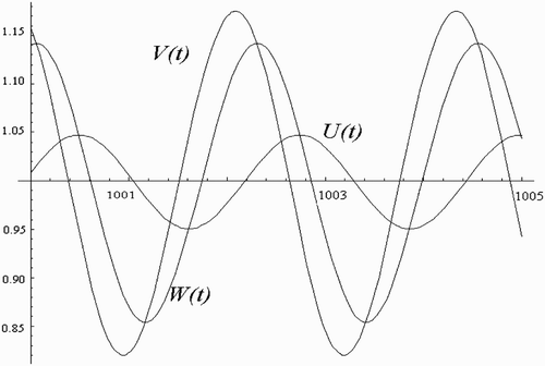
We use a step-by-step procedure, as explained in 4, to completely determine the nature of the periodic solutions arising from the Hopf bifurcation. Tedious but straightforward computations yield the approximation solutions

where

and

with

For the parameter values , and τ=4, we obtain the following values for the period, the amplitudes, and the characteristic exponent, respectively:

Figure 14 shows the graph of the periodic solutions plotted in the system of coordinates (u, v, w) with respect to time t, where . Observe that these solutions are positive and bounded around the steady state .

Figure 14. Graph representing the behaviour of the periodic solutions u(t), v(t), and w(t) in the system of coordinates (u, v, w) with respect to time (t _min=1000, t _max=1005).

5. Conclusion and discussion

A mathematical model, originally introduced by Ngwa 12 to study the population dynamics of the malaria vector, was extended to include spatial component and dispersal in which vectors, from different breeding sites, can visit host habitats within their flight range domain and interact with them. During the interaction, the vectors can be successful, fail and seek to try again, or fail and be killed. In our modelling, the vectors were assumed to be located at N breeding sites spatially distributed among M human habitats. Vector deaths prior to the adult vector stage and a delay factor T were taken into consideration in the modelling. Analysis of the model equations under a given set of defined assumptions and using a Verhulst–Pearl birth function for the vectors led to the following results:

• (1) There is always a unique non-zero steady-state distribution of humans over the number of human habitats, which is globally and asymptotically stable for all reasonable parameter values.

• (2) For the vector population, a trivial steady-state solution always exists. In addition, there is a non-trivial steady-state vector distribution whose existence is uniquely determined by a threshold parameter . When the threshold parameter , there exists exactly one real positive non-trivial steady state solution, and if the only steady state is the trivial steady state. The non-trivial steady states were obtained for different distributions of the vector-breeding sites.

• (3) Furthermore, for the one-human habitat, one-vector-breeding site scenario with no time delay, Ngwa 12 partially established the presence of a Hopf bifurcation in a particular parameter space. Here, we use a step-by-step procedure, as explained in 4, to completely determine the nature of the periodic solutions arising from the Hopf bifurcation.

The modelling techniques used can be applied to analyse the dynamics of many different vectors. In addition, the results obtained can be very useful in designing effective control strategies aimed at fighting and eradicating vector-borne diseases. Two major ways in which disease vectors can be controlled are chemical or biological. Biological control of vectors can be realized by the introduction of a predator (i.e. another organism which feeds on the vectors) at the vector breeding site. For example, in the case of swamp insect vectors, control can be implemented by the introduction of a species of fish which feeds on the larvae of the vectors. Usually, the effectiveness of this kind of control is long term, since the predator needs some time to establish itself in the environment. On the other hand, chemical control can be realized through direct application of a chemical and toxic substances in the vectors themselves or in their breeding sites, in order to interrupt their reproduction cycle. For example, pesticides like DDT and toxic bed nets are used to control mosquitoes and midges (see 16 for more on human disease vectors and their control measures). Therefore, understanding vector dynamics is crucial in the understanding how both biological and chemical control can impact vector-borne disease control. For example, continuous application of control measures (use of insecticides, bed nets, specialized candles, and mosquito traps 10) when the vector population is at its minimum amplitude may result in a decrease in the growth of the vector population and possible extinction in extreme cases. On the other hand, the application of control measures when the population is at its peak may not be an efficient strategy.

The model presented is the first to the best of our knowledge, and just the first step in completely understanding the population dynamics of vectors when there is more than one breeding site interacting with the host habitat. This is very important especially when applied to the Anopheles mosquito, the vector that transmits the malaria-causing agent – plasmodium. In order to control malaria, multiple interventions are needed 18 19 which involve a combination of: vector control 12; reduction of contact between humans and vector 17; control of the infectious agent, Plasmodium, both within the human host 19 and the vector 18; and education (of the people that are most affected) 17 and control of the vector-breeding sites. Hence, our paper seeks to further the understanding of the vector population dynamics which could assist in the planning and implementation of new malaria intervention and vector control strategies.

Many extensions exist, some of which are currently under investigation, and include the following:

• (1) Analysing the stability of the steady states obtained.

• (2) Using a shorter method of establishing the existence of steady states for any number of vector-breeding sites and human habitats, and obtaining an explicit form of the steady states and analysing their stability.

• (3) Incorporating the fact that many of the vector-breeding sites are dynamic. In most endemic regions such as Cameroon, breeding sites are created due to muddy ponds and washed out due to heavy rains or dried up due to high heat. Hence, most of the breeding sites very close to human habitats are temporal and created at some rate and destroyed at some rate [21 . Therefore, incorporating the lifespan of breeding sites and the dynamics of their formation and destruction into our model will prove very crucial in understanding mosquito dynamics and will be important in control measures at eradicating vector-borne diseases that are transmitted by vectors that live in breeding sites and rely on host habitats for their main sustenance and survival.

• (4) Incorporate predation at the vector-breeding sites and see what the impact to the mosquito dynamics will be.

• (5) Include disease dynamics in the model in which questing vectors that feed successfully can in the act transmit an infectious agent that can cause a disease or be infected with an infectious agent that can again be transmitted at a later feeding.

Acknowledgements

The first author (S. Nourridine) and the third author (G.A. Ngwa) wish to acknowledge support of a grant from the Faculty of Science, University of Buea, Cameroon, under the Faculty of Science Research Grant Scheme 2008/2009. The second author (M.I. Teboh-Ewungkem) wishes to acknowledge support of the NSF Grant Award No. OISE-0855380 that made it possible for all three authors to meet and to work at the University of Buea. All three authors will like to thank the reviewers for their time in reading this paper.

Notes

These are usually blood-sucking athropods.

It could be a virus, protozoa, bacteria, fungi, or helminth.

By host we mean the organism infected by the infectious agent and which interacts with the vector.

These are vectors with a preference for human blood. If the vectors have a preference to animal blood, they are said to be zoophilic.

It is understood that once the infectious disease is involved and accounted for in the model, e.g. when either the vector or human is infected, then this assumption must be relaxed.

Human's blood preference factor of the vectors (H=human density).

Animal's blood preference factor of the vectors (A=animal density).

References

- Brännström , Å. and Sumpter , D. J.T. 2005 . The role of competition and clustering in population dynamics . Proc. R. Soc. B. , 272 : 2065 – 2072 .
- Githeko , A. K. , Lindsay , S. W. , Confalonieri , U. E. and Patz , A. J. 2000 . Climate change and vector-borne diseases: A regional analysis . Bull. World Health Organ. , 78 ( 9 ) : 1136 – 1147 .
- Gubler , D. J. , Reiter , P. , Ebi , K. L. , Yap , W. , Nasci , R. and Patz , A. J. 2001 . Climate variability and change in the United States: Potential impacts on vector - and rodent-borne diseases . Environ. Health Perspect. , 109 ( 2 ) : 223 – 233 .
- Hassard , B. D. , Kazarinoff , N. D. and Wan , Y.-H. 1981 . Theory and Applications of Hopf Bifurcation , Vol. 41 , Cambridge : Cambridge University Press . London Mathematical Society Lecture Note Series, London
- Jang , S. R.J. 2005 . Contest and scramble competition with a dynamic resource . Nonlinear Anal. , 63 : 109 – 118 .
- Martens , W. J.M. , Jetten , T. H. , Rotmans , J. and Niessen , L. W. 1995 . Climate change and vector-borne diseases: A globally modelling perspective . Global Environ. Change , 5 : 195 – 209 .
- Martens , P. , Kovats , R. S. , Nijhof , S. , de Vries , P. , Livermore , M. T.J. , Bradley , D. J. , Cox , J. and McMichael , A. J. 1999 . Climate change and future populations at risk malaria . Global Environ. Change A , 9 : S89 – S107 .
- McCall , P. J. and Kelly , D. W. 2002 . Learning and memory in disease vectors . Trends Parasitol. , 18 ( 10 ) : 429 – 433 .
- McKenzie , F. E. and Bossert , W. H. 1997 . The dynamics of Plasmodium falciparum blood-stage infection . J. Theor. Biol. , 188 ( 1 ) : 127 – 140 .
- Mosquito Solutions . Dragonfly Mosquito System(R); available at http://www.cdc.mosquitosolutions.com (accessed May 2009)
- Ngwa , G. A. 2004 . Modelling the dynamics of endemic malaria in growing populations . Discrete Contin. Dyn. Syst. Ser. B , 4 ( 4 ) : 1173 – 1202 .
- Ngwa , G. A. 2006 . On the population dynamics of the malaria vector . Bull. Math. Biol. , 68 : 2161 – 2189 .
- Ngwa , G. A. and Shu , W. S. 2000 . A mathematical model for endemic malaria with variable human and mosquito populations . Math. Comput. Model. , 32 ( 7–8 ) : 747 – 763 .
- Ngwa , G. A. , Ngonghala , C. N. and Sama Wilson , N. B. 2001 . A model for endemic malaria with delay and variable populations . J. Cameroon Acad. Sci. , 1 ( 3 ) : 168 – 186 .
- Schmidt , G. D. and Roberts , L. S. 1989 . Foundations of Parasitology , 4 , Times Mirror/Mosby College Publishing .
- J.D. Smyth, Animal Parasitology, Low Price Edition, Vol. 19(1), Cambridge University Press, Cambridge, 1996
- Teboh-Ewungkem , M. I. 2009 . “ Malaria control: The role of local communities as seen through a mathematical model in a changing population-Cameroon ” . In Advances in Disease Epidemiology , Edited by: Tchuenche , J. M. and Mukandavire , Z. 103 – 140 . New York : Nova Science Publishers .
- Teboh-Ewungkem , M. I. and Yuster , T. 2010 . A within-vector mathematical model of Plasmodium falciparum and implications of incomplete fertilization on optimal gametocyte sex ratio . J. Theor. Biol. , 264 ( 2 ) : 273 – 286 .
- Teboh-Ewungkem , M. I. , Podder , C. N. and Gumel , A. B. 2010 . Mathematical study of the role of gametocytes and an imperfect vaccine on malaria transmission dynamics . Bull. Math. Biol. , 72 ( 1 ) : 63 – 93 .
- Teboh-Ewungkem , M. I. , Yuster , T. and Newman , N. H. 2010 . “ A mathematical model of the within-vector dynamics of the Plasmodium falciparum protozoan parasite ” . In Infectious Disease Modelling Research Progress , Edited by: Tchuenche , J. M. and Chiyaka , C. 177 – 199 . New York : Nova Science Publishers .
- Wanji , S. , Mafo , S. S. , Tendongfor , N. , Tanga , M. C. , Tchuente , F. , Bilong Bilong , C. F. and Njine , T. 2009 . Spatial distribution, environmental and physicochemical characterization of Anopheles breeding sites in the Mount Cameroon region . J. Vector Borne Dis. , 46 : 75 – 80 .
- WHO . World malaria report, 2008. Available at http://www.int/malaria/publications/atoz/9789241563697/en/index.html (accessed May 2010)