Coexistence of competitors in deterministic and stochastic patchy environments

Abstract

The spatial component of ecological interactions plays an important role in shaping ecological communities. A crucial ecological question is how does habitat disturbance and fragmentation affect species persistence and diversity? In this paper, we develop a deterministic metapopulation model that takes into account a time-dependent patchy environment, thus our model and analysis take into account environmental changes. We investigate the effects that spatial variations have on persistence and coexistence of two competing species. In particular, we study the local behaviour of the model, and we provide a rigorous proof for the global analysis of our model. Also, we compare the results of the deterministic model with simulations of a stochastic version of the model.

Keywords:

• metapopulation
• patch dynamics
• species competition
• coexistence
• stochasticity

1. Introduction

Understanding the impact of space on species coexistence is a major topic in theoretical and experimental ecology studies 23. Over the past decades, lots of mathematical models have been used to study the impact of spatial heterogeneity on population dynamics of systems of interacting species (see, e.g. 6 8 14 30 35). These studies have demonstrated that spatial structure is at least as important as birth and death processes, competition, or predation 35. For example, spatial structure is known to allow two competing species to coexist 30; stabilize predator–prey dynamics 9 14, and influence the evolution of cooperative behaviour 24.

There are several ways of incorporating spatial heterogeneity or patchiness into population models 6. Space is implicitly included in spatially structured metapopulation models, such as the Levins model 16. These models focus on changes in patch occupancy as a function of rates of patch colonization and extinction. However, these models have no spatial dimension and portray patches as equally accessible to one another 26. More recently, the spatially structured metapopulation models have been used extensively in studies of formation and conservation of biodiversity. Furthermore, extensions of these models have been used to describe multi-species intraspecific competition in patchy environments 6 7 8 30 35. Metapopulation models are known to have many characteristics that are similar to those of epidermic models 2 3 4 5 20 if empty and occupied ‘patches’ are represented as susceptible and infected individuals, respectively. Therefore, some typical results and terminologies in epidemiology will be used in this paper.

In 1983, Hanski and Ranta 8 formulated a two-species model to study intraspecific competition in water fleas of the genus Daphnia. In their model, the rate of appearance of new habitable patches is assumed to be constant, and the dynamic process of patch destruction and recreation is ignored. In real systems, however, habitable patches may be destroyed while destroyed patches may become habitable again. The rates at which these events occur may depend on many factors including climate changes, environmental conditions, or human activities. Thus, to capture this biological reality, we incorporate patch dynamics into our deterministic metapopulation model. Another major contribution of our study is that we provide a detailed analysis for the global stability of the system. Our analysis provides significant insights into the outcomes of species competition. The local stability analysis in Hanski and Ranta 8 is only applicable to special cases, and the stability conditions (based on the Routh–Hurwitz criteria ) do not provide biological insights, and the conditions for coexistence are only verified by numerical simulations instead of a rigorous mathematical proof. It should be noted that the approaches used in this paper are very general and can be used to analyse the global dynamics of the model formulated in Hanski and Ranta 8.

Real biological systems are inevitably subject to stochastic interference. Demographic stochasticity and environmental stochasticity are two familiar types of stochasticity that may significantly affect a biological system. Demographic stochasticity is the temporal variance in population density caused by randomness in the reproduction and mortality of individuals 30, and environmental stochasticity is the stochastic variation in the physical and biological environment and thereby in the parameters affecting the system. Many epidemiological and ecological models with demographic or environmental stochasticity have been studied in the past few decades (see, e.g. 1 17 18 19 25 32). In this paper, we incorporate such stochastic factors in our model and examine how these factors may influence the persistence and coexistence of two competing species.

The paper is organized as follows. In Section 2, we formulate the deterministic model. The model describes changes in the state of patches. Section 3 is focused on stability analysis of the deterministic model. In Section 3, we prove the local dynamics of the boundary steady states. Furthermore, we prove that under certain conditions on the ‘invasion reproductive number’ the model is uniformly persistent. That is, we obtain conditions that guarantee the coexistence of competing species in a deterministic patchy environment. In addition, we prove a global stability result for the deterministic model. In Section 4, we introduce two stochastic models that are based on the deterministic model. We investigate the impact of environmental stochasticity and demographic stochasticity on the persistence and coexistence of two competing species. We compare the dynamics of the deterministic model with that of two stochastic models. The paper ends with a brief discussion of our results in Section 5.

2. Deterministic model

Our deterministic model follows Levin's framework for metapopulation model, which in the case of a single species has the form

where p(t) denotes the proportion of occupied patches at time t, c is the per capita colonization rate of empty patches, and e is the per capita extinction rate of occupied patches. This model assumes an infinite network of homogeneous patches and is spatially implicit. A classic result provided by this model is that metapopulation persistence is possible if and only if the colonization rate exceeds the critical threshold set by the extinction rate. This model has been extended to include two interacting species 8 12 15 21 22 or multiple species 10 11 15 30.

Although our model has a similar structure as that in Hanski and Ranta 8, there are some key differences between the two models. One of the most significant differences between their study and ours lies in the biological insights obtained from the analytical results of the models. In terms of the model structure, their model includes a per capita rate (ν) of pool (patch) disappearance and a constant rate q of appearance of new pools (patches). Under this assumption, the total number of pools (N) satisfies the equation , and is asymptotically a constant (q/ν). Our model assumes a constant per capita patch destruction rate d (i.e. the rate at which a habitable patch becomes nonhabitable) and a constant per capita patch recreation rate r (i.e. the rate at which an nonhabitable patch becomes habitable). Under this assumption, the number of nonhabitable and habitable patches are time-dependent while the total number of patches remain constant for all time.

The analytic results of the model in Hanski and Ranta 8 and our model include the stability analysis of the nontrivial boundary equilibria (i.e. equilibria at which only one species is present). It is pointed out in Hanski and Ranta 8 that the local stability conditions expressed by (6c) and (6d) can be written down using the model parameters but they are uninformative. Consequently, they considered only some special cases of the expression. Our model allows us to derive general stability conditions for the system equilibria and are much more informative. Particularly, our results can be used to compute the criteria for one species to invade a metapopulation in which the other species has already established itself, as well as to examine the role of patch dynamics (destruction and recreation) on species invasion and coexistence. Moreover, our analytical results include both the local and the global stabilities of the nontrivial boundary equilibria as well as the uniform persistence of the metapopulations of both species.

In our two-species metapopulation model, we divide the total number of patches into five subtypes of patches. The fractions of these five types of patches are denoted by: u ₀ for nonhabitable patches (or destroyed); u ₁ for habitable but empty (i.e. not colonized by either species); x for patches occupied by species 1 only; y for patches occupied by species 2 only; and z for doubly occupied patches (i.e. occupied by both species 1 and species 2). The transition diagram between patch states is shown in Figure 1. Patch destruction occurs at a constant per capita rate d, and nonhabitable patches can become habitable at a constant per capita rate r. Species i (i=1, 2) colonizes an empty patch at the per capita rate c _i , and it goes extinct in a patch absent of the other species at the per capita rate e _i . A patch that is occupied by species i can be colonized by species j (j≠i) at the per capita rate k _j c _i with k _j ≤1 (which represents the assumption that the colonization of a patch occupied by the other species is more difficult than the colonization of an empty patch). If a patch is doubly occupied, then there may be an extra extinction rate for species i so that the total extinction rate is . All our model parameters are nonnegative. The definitions of all variables and parameters are summarized in Table 1. The model is described by the following system of differential equations:

Using the fact that , we can ignore the u ₀ equation in system (1) and consider the following equivalent four-dimensional system:

Our analytical results will be conducted using system (2).

Figure 1. Transition diagram between patch states. Nonhabitable patches and empty habitable patches correspond to u ₀ and u ₁, respectively. Patch dynamics are governed by destruction and creation rates d and r, respectively. Metapopulation dynamics are governed by colonization rates c _i and k _ij and extinction rates e _i and ε _i .

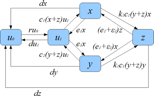
Table 1. Model parameters.

Parameter	Description
c i	Species i colonization rate of an empty patch
e i	Species i extinction rate in a patch occupied by a single species
	Species i extinction rate in a patch occupied by two species
k ij ∈(0, 1)	Species i colonization rate of a patch occupied by species j
d	Constant rate of patch destruction
r	Constant rate of patch creation

Adding all the equations in system (2) yields

From the above equation, we know that as , where

represents the long-term proportion of habitable patches. Assume that the system has reached the asymptotic state, i.e.

Then, the biologically feasible region for system (2) is

It can be verified that Γ is positively invariant, and that the usual results on the existence and uniqueness of solutions as well as the continuation results hold. In the following sections, we restrict our analysis to solutions with initial conditions in Γ.

3. Stability analysis

System (2) always has the trivial (species-free) equilibrium

There are two possible nontrivial boundary equilibria at which only one species is present:

where

and

Clearly, E _i is biologically feasible (i.e. the components are between 0 and 1) only if the following quantities

are sufficiently large or more specifically, if the following conditions hold

Note that c _i is the rate at which species i colonizes a habitable and empty patch, 1/(e _i +d) is the mean time of patch occupancy by species i (in the absence of the other species), and p is the long-term fraction of habitable patches. Thus, ℛ _i gives the long-term expected ‘reproduction number’ of species i in a landscape where the proportion of habitable patches is p.

3.1. Local stability and invasion criterion

The following results show that the reproduction numbers ℛ₁ and ℛ₂ also determine the stabilities of the equilibria E _i , i=0, 1, 2.

Theorem 1

Let ℛ _i be defined as in Equation (6). Then

• (i) E ₀ is globally asymptotically stable (g.a.s.) if for i =1, 2, and it is unstable if or ;

• (ii) E _i is g.a.s. if and only if and for i, j=1, 2 and j≠i.

Proof

Proof of part (i). Since k ₁<1, adding the second and fourth equations of system (2) gives

From the above inequality and , we have as ; and thus, and as . Similarly, it can be shown that if then and as . Therefore, if for i=1, 2, then E ₀ is globally asymptotically stable. This completes the proof of part (i). For the proof of part (ii), noticing the mathematical symmetry between species 1 and 2, we only need to prove the results for the case of i=1. From the proof of part (i), we know that if then and as . Thus, the limiting system of (2) is

Let denote the nontrivial equilibrium of system (7). Then the stability of E _1l is equivalent to the stability of E ₁ for system (2). It is easy to show that E _1l is locally asymptotically stable (l.a.s.) when . For the global stability of E _1l , let (f ₁, f ₂) be the vector field defined by system (7). Then using the Dulac function D(u ₁, x)=u ₁ x and noticing that x<1, we have

Thus, system (7) does not have a limit cycle. Notice that the trivial equilibrium (u ₁, x)=(0, 0) of system (7) is unstable as , and that E _1l is the only nontrivial equilibrium of system (7). Therefore, E _1l is g.a.s. It follows that the boundary equilibrium E ₁ of system (2) is g.a.s. Using a similar argument, we can show that E ₂ is g.a.s. when and . This completes the proof.   ▪

Next, we consider system (2) in the case of and . In this case, both E ₁ and E ₂ exist. However, their stabilities will now depend on other conditions. In fact, these conditions can be written in terms of the following quantities:

where

The biological interpretations of the quantities and are given in Section 3.3.

The local stability results for E _i (i=1, 2) are described in the following theorems.

Theorem 2

Let and be as defined in Equations (8) and (9), respectively.

• (a) If then the boundary equilibrium E ₁ is l.a.s. (unstable).

• (b) If then the boundary equilibrium E ₂ is l.a.s. (unstable).

Proof

Due to the mathematical symmetry between the two species, we only need to present a proof for Part (a) of this theorem. The Jacobian matrix of system (2) at E ₁ is

The top-left 2×2 block matrix has two negative eigenvalues

For the bottom-right 2×2 block matrix, the trace is

and the determinant is

It can be shown that if A>0 then B<0. Thus, B>0 implies that A<0. We can also verify (with extensive algebraic calculations) that B>0 if and only if . Therefore, E ₁ is l.a.s. if , and it is unstable if . This completes the proof of Part (a) of Theorem 2. Part (b) can be proved in a similar way.   ▪

The following theorem provides a result concerning the uniform persistence of both species, i.e. there exists a constant δ>0, which is independent of initial data, such that

Theorem 3

If and then system (2) is uniformly persistent and has a positive equilibrium.

Proof

Define

It suffices to show that system (2) is uniformly persistent with respect to 34. It is easy to see that both X and X ₀ are positively invariant. Clearly, ∂ X ₀ is relatively closed in X and system (2) is point dissipative. Set

with also satisfying Equation (2). We first show that

where and Let . To show that Equation (10) holds, it suffices to show that we have either x(t)=0 and z(t)=0, or y(t)=0 and z(t)=0 for all t≥0. Suppose this is not true. Then there exists a t ₀≥0 such that, without loss of generality, , and z(t ₀)=0 (other cases can be discussed in the same way). Assume that u ₁(0)>0 (a reasonable assumption), then it follows that u ₁(t)>0 for all t>0. Since

it follows that there is an such that z(t)>0 for . Clearly, we can restrict to be small enough so that , and u ₁(t ₀)>0 for . This means that for , which contradicts the assumption that . Hence, this shows that Equation (10) holds. Using the same argument as in the proof of Theorem 1, we know that E _i is a global attractor in for system (2) (i=1, 2). It then follows that the set {E ₀, E ₁, E ₂} is isolated and is an acyclic covering in ∂ X ₀. By Theorem 4.6 in Thieme 29, we only need to show that , , and when and . To show that , we notice that the conditions and imply that and . Thus, we can choose δ small enough such that

Assume that . Then there exists a positive solution with such that as . Then, for t sufficiently large, we have , and

Since (from the inequality (11)), by the comparison principle 27 we have as . This contradicts as , implying that . We now show that when . Since and hence B<0, we can choose η>0 small enough such that

Assume that . Then there exists a positive solution with such that as . Thus, for t sufficiently large we have and

Consider the following auxiliary system

The coefficient matrix Ĵ of system (13) is given by

Since Ĵ has positive off-diagonal elements, from the Perron–Frobenius theorem we know that there is a positive eigenvector v _m corresponding to the maximum eigenvalue λ _m of Ĵ. After extensive computations, we have λ _m >0 since Equation (12) holds. Using linear systems theory, we can show that all positive solutions of Equation (13) tend to infinity as t→∞. Then, applying the standard comparison principle we have and as . This contradicts as , implying that . The case for can be proved in a similar way. Finally, from , , , and the fact that the set {E ₀, E ₁, E ₂} is acyclic in ∂ X ₀, we can apply Theorem 4.6 in Thieme 29 and conclude that system (2) is uniformly persistent with respect to . Using Theorem 1.3.7 in Zhao 36 as applied to the solution semiflow of systems (2), we can immediately obtain that the system has a positive equilibrium. This completes the proof of Theorem 3.   ▪

3.2. Global analysis of the coexistence equilibrium

In this section, we mainly consider the case when the extra extinction rates in doubly occupied patches are ignored, i.e. . In this case, it is convenient to use the variables n ₁=x+z and n ₂=y+z (in stead of x and y). Note that n _i represents the total proportion of patches with species i (i=1, 2). System (2) can be rewritten as

Noting that

as , we can consider the limiting system of Equation (14):

For system (15), the trivial equilibrium and the two nontrivial boundary equilibria are

where and . Notice that these equilibria are the same as the corresponding ones for system (2), and we have used the same notation E _i (i=0, 1, 2). From Theorem 1, we can easily see that the global asymptotic behaviours of system (15) remain the same for the case of or . Thus, for the remaining analysis in this section, we assume that and , i.e.

Notice that for the invasion reproduction numbers and (given in Equations (8) and (9)) now simplify to

and

Let

It is easy to verify that all solutions of system (15) starting in Γ will remain in Γ for all t≥0. Hence, Γ is positively invariant. Thus, in this section, our analysis will be carried out for system (15) in Γ. Since for i=1, 2, it follows that

Therefore, we must have either or .

Let denote a positive equilibrium of system (15), i.e. , , and z*>0. We can find E* by solving the following algebraic equations:

Using the first and second equations in (18) we have

From Equation (19) and the third equation of (18) we know that z* satisfies the following quadratic equation

where

Thus, the components of E* are given by

where B ₁, B ₂, B ₃ are defined in Equation (21).

The existence (or nonexistence) condition of E* is described in the following theorem.

Theorem 4

Let denote a positive equilibrium of system (15). Then

• (i) E* does not exist if and , or if and ;

• (ii) E* exists and is unique if and . Moreover, and z* are given by Equation (22).

Proof

For the proof of part (i), we only pick up the case to prove the theorem. If , the theorem can be proved in a similar way. If we have B ₃<0 and

It follows that

and

We claim that B ₂<0. In order to prove the claim, we consider three cases, i.e. , and .

Case 1

. In this case, it is easy to see that B ₂<0 since

and

Case 2

. In this case, since

we have

Case 3

. In this case, we have

Since B _i <0, i=1, 2, 3, it is easy to see that Equation (20) has no positive solution. Therefore, when , system (15) has no positive equilibrium. This finishes the proof of part (i).

Proof of Part (ii). As and , we have B ₁<0 and B ₃>0. It then follows that Equation (20) has at most one positive solution

Consequently, system (15) has at most one positive equilibrium . On the other hand, system (20) is uniformly persistent for and . This implies that system (15) has at least one positive equilibrium. Therefore, when and , system (15) has a unique positive equilibrium , where and z* are given by Equation (22). This finishes the proof of part (ii). The proof of Theorem 4 is completed.   ▪

The next result concerns the global stabilities of the nontrivial equilibria E ₁ and E ₂. For these global dynamics of system (15), we need to first mention some results from Jiang et al. 13 concerning three-dimensional K-competitive dynamical systems.

Consider the system of differential equations:

It follows from Smith 27 that a matrix A is called type K-competitive and irreducible if A has the following form

where the ‘*’ represents an arbitrary element. System (23) is called type K-competitive and irreducible if the Jacobian Df(x) of f is type K-competitive and irreducible for each . Set

It follows from the Perron–Frobenius theorem that A has a real eigenvalue, which has a unique unit eigenvector in Int K, and the real parts of the other two eigenvalues are strictly greater than this real eigenvalue if A is type K-competitive and irreducible.

We also need to introduce the following concepts. A vector x is called K-positive if x∈K, and it is called strictly K-positive if . Two distinct points are K-related if either u−v or v−u is strictly K-positive. A set S is called K-balanced if no two distinct points of S are related.

Notice that the Jacobian of system (15) is

It can be verified that system (15) is K-competitive in Γ. From the expressions of , , z*, x¯, and [ytilde], it is not difficult to see that the equilibria E ₁ and E ₂ (or E ₁, E ₂, and E*) are unordered in the K-order. It follows from Proposition 3.2 in Wang and Jiang 33 and Proposition 1.3 in Takac 28 that there exists a two-dimensional compact Lipschitz submanifold Σ such that , or and . Moreover, Σ is K-balanced. Since Σ is a two-dimensional compact Lipschitz submanifold and homeomorphic to a compact domain in the plane, it is obvious that the Poincare–Bendixson theorem holds for the dynamics of system (15) on Σ.

Notice that system (15) has only two boundary equilibria E ₁ and E ₂, and from Theorems 2 and 3 we know that E ₁ is stable and E ₂ is unstable when and . Since there is no positive equilibrium, from the Poincare–Bendixson theorem we know that E ₁ is g.a.s. Using a similar way, we show that E ₂ is g.a.s. if and . Therefore, the following result holds.

Theorem 5

If and then the nontrivial boundary equilibrium E _i of system (15) is g.a.s.

Although we do not have an analytic result for the stability of the interior equilibrium E*, the results in Theorems 1 – 6 suggest that E* is l.a.s. when and . Biological interpretations of these results are provided in the next section.

3.3. Biological interpretations of the results

In the previous sections, we proved several results regarding the local and global dynamics of system (2) including the existence and stability of the equilibria E ₀, E ₁, E ₂, and E*. We point out that these results have been described using the quantities ℛ _i and (i, j=1, 2 and i≠j), which are defined in Equations (6), (8), and (9). These quantities have clear biological meanings. For example, is the product of c _i (the rate that species i colonize a habitable and empty patch), 1/(e _i +d) (the mean time that a patch is occupied by species i in the absence of the other species), and p (the fraction of habitable patches). Thus, ℛ _i gives the expected ‘reproduction number’ of species i in a landscape where the proportion of habitable patches is p. If a landscape is completely habitable, i.e. if p=1, then the ‘basic reproduction number’ of species i is

To see the meaning of more easily, we ignore the extra extinction rate for doubly occupied patches (i.e. ). In this case, from Equations (8) and (9) we can simplify the expressions for and as

where ū ₁, x¯, ũ ₁, and [ytilde] are given in Equations (4) and (5). Notice that is the species 1-only equilibrium and is the species 2-only equilibrium. Thus, gives the reproduction number of species j in a landscape in which only species i (j≠i) is present. We term the ‘invasion reproduction number’ of species j. The result in Theorem 2 implies that species 2 can invade the metapopulation of species 1 only if the invasion reproduction number exceeds 1.

Combining the results in Theorems 1–5, we can draw the following conclusions for the competition outcomes of the two species:

These conditions make clear biological sense from the meaning of ℛ _i and . Comparing with the corresponding results in Hanski 6 in which the conditions for nontrivial equilibria cannot provide explicit biological interpretations due to the complexity of the expressions, our results are more useful in terms of gaining biological insights.

It is also helpful to rewrite the invasion condition in Equation (25) in terms of ℛ₁ and ℛ₂:

and

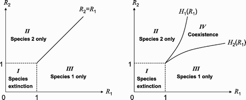
Since the equilibrium E _i exists if and only if (i=1, 2), and from , and , we know that the curve is above the curve for , except that in the case of k ₁=k ₂=0 (i.e. no doubly occupied patches). Moreover, the two curves intersect at . Bifurcation diagrams for these two cases are shown in Figure 2. It is shown in Figure 2 that coexistence is very unlikely if no patches can be cooccupied by both species (the left figure), and there are three regions (labelled by I, II, and III) formed by the lines and by the curves (i=1, 2) representing species extinction (Region I), species 1 only (Region II), and species 2 only (Region III). If double occupancy is allowed, then there is a region for coexistence (Region IV).

Figure 2. (ℛ₁, ℛ₂) plane. The left figure is for the case when there is no doubly occupied patches (k ₁=k ₂=0) and the right figure is for the case k ₁>0 and k ₂>0. The two curves ℛ₂=H ₁(ℛ₁) and ℛ₂=H ₂(ℛ₁) are determined by the invasion conditions ℛ _ij >1 (i, j=1, 2, i≠j). Both species will go extinct if ℛ _i <1 (i=1, 2), i.e. if (ℛ₁, ℛ₂) is in Region I. Only species 1 will be present if (ℛ₁, ℛ₂) is in Region II, and only species 2 will be present if (ℛ₁, ℛ₂) is in Region III. Both species will coexist if (ℛ₁, ℛ₂) is in Region IV.

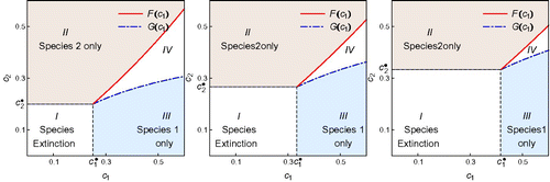
These results can be used to examine the role of various ecological factors play in the competitive outcomes of metapopoulation. For example, from the threshold value we can derive a threshold value of colonization rate ,

such that if and only if . Similarly, the conditions and are equivalent to, respectively,

and

where p=r/(r+d) is the long-term proportion of habitable patches.

Using Equations (29)–(31), we can draw a bifurcation diagram in the (c ₁, c ₂) plane. Moreover, these conditions allow us to examine how the model parameters such as p (the long-term proportion of habitable patches) and e _i (patch extinction) may affect the competition outcomes. For example, the effect of p is illustrated in Figure 3, in which the three plots are for the values of p=1 (left), p=0.75 (middle), and p=0.6 (right). We observe that as p decreases (i.e. as the fraction of habitable patches decreases), the region for the extinction of both species increases significantly while the coexistence of two species becomes much less likely. It also suggests that the negative impact of decreasing p is higher on species 1 than on species 2. The parameter values used in this figure are e ₁=0.15, e ₂=0.1, k ₁=0.1, and k ₂=0.4.

Figure 3. Regions of competition outcomes in the first quadrant of the (c ₁, c ₂) plane for different values of p, the long-term proportion of habitable patches. The four regions are: (i) species extinction if for i=1, 2, where the threshold values and are given in Equation (29), i.e. if (c ₁, c ₂) is in Region I; (ii) species 1 only if (c ₁, c ₂) is in Region II; (iii) species 2 only if (c ₁, c ₂) is in Region III; and (iv) coexistence of both species if (c ₁, c ₂) is in Region IV. The left figure is for the case p=1 (i.e. all patches are habitable). The middle and right figures are for the cases p=0.8 and p=0.5, respectively. It shows that as p decreases, the region of extinction increases significantly while the region of coexistence becomes much smaller. It also suggests that the negative impact of decreasing p is higher on species 1 than on species 2.

4. Stochastic simulations

To explore the impact of stochastic factors on the system behaviours, we conducted stochastic simulations of the system, and the results from the deterministic model and stochastic simulations are compared. Guided by the theoretical results from the deterministic model, we consider stochasticity in several parameters that may have important influence on the dynamics of the system. For example, the effect of environmental stochasticity is examined by considering random parameters including the species i, i=1, 2 colonization rate of empty patch c _i , the extinction rate e _i , the colonization rates of occupied patch k ₁₂ and k ₂₁, and the rates of patch destruction d and recreation r. For simplicity, our basic model describes the dynamics of a metapopulation without keeping track of the local population dynamics for species within each patch. That is, a habitable patch is considered either empty or occupied, and there is no detailed description for the population growth within an occupied patch. Consequently, there is no demographic stochasticity.

In this section, we present three scenarios based on the competitive outcomes of the two species identified from the analysis of the deterministic model. There the scenarios correspond to the three cases are listed in Equation (26). We first consider the case when the rates of colonization (c _i ) and extinction (e _i ) are random parameters, which are assumed to be uniformly distributed.

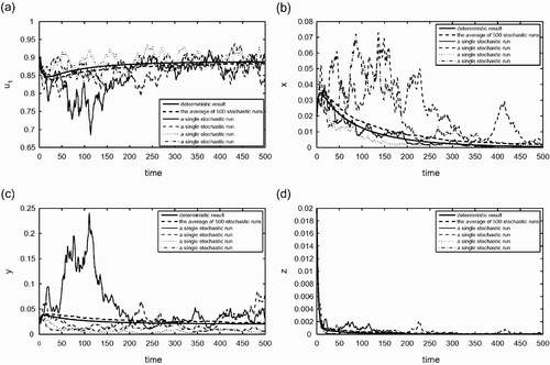
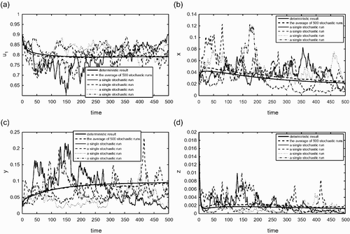
In Figure 4, and , which corresponds to the case (i) described in Equation (26) with i=2 and j=1. Thus, the deterministic outcome is that only species 2 will be present. Time variations of the variables x, y, z, u ₁ are presented in these figures. Figure 4 shows the average of 500 stochastic runs (the dashed curve) and the solution curve of the deterministic model (the solid curve), whereas Figure 4 illustrates four individual stochastic runs (thin curves) together with the deterministic curve (the solid curve). We see from Figure 4 that the average behaviour of the stochastic simulations is very similar to that of the deterministic simulation. More diverse outcomes can also be observed in Figure 4. There are individual runs that exhibit coexistence of the two species (e.g. see the solid blue curve), and other runs show that both species go extinct (see the solid red curve).

Figure 4. Stochastic simulations with c _i and e _i as random parameters (see the text for more detailed explanations). (a) The fraction of habitable but empty patches; (b) the fraction of patches occupied by the species 1 only; (c) the fraction of patches occupied by the species 2 only; (d) the fraction of patches occupied by both species 1 and 2. The random parameters are again c _i , e _i , i=1, 2, k ₁₂, k ₂₁, d, and r. The solid curve represents the solution curve of the deterministic model and the dash thick curve shows the average of 500 stochastic runs. The thin (solid, dashed, dot, dashed, and dot) curves show four individual stochastic runs. The parameter values used for the deterministic simulation, which are the mean values of the random variables in the stochastic runs, are: c ₁=0.17, c ₂=0.18, e ₁=e ₂=0.15, r=0.1, d=0.01, ε₁=ε₂=0.01. For this set of parameter values, ℛ₁=0.9659, ℛ₂=1.0227, ℛ₁₂=1.0408, and ℛ₂₁=0.9552. This corresponds to the case (i) listed in Equation (26). In this case, the deterministic outcome is that only species 2 will be present. We observe that the average behaviours of stochastic simulations is very similar to the behaviour of the deterministic model. The outcomes of some individual runs, for example the solid thin curves, may be very different from the average outcome in some relative short time periods.

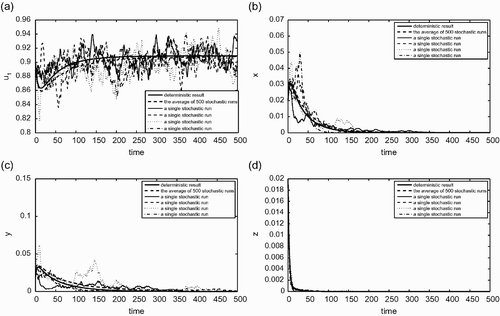
Figure 5 is similar to Figure 4, but for the case (ii) described in Equation (26). That is, and (i, j=1, 2 and i≠j). In this case, the deterministic outcome is coexistence of both species. We see from Figure 5 again that the average behaviour of the stochastic simulations is very similar to that of the deterministic simulation. The individual runs shown in Figure 4 include both the case when species 1 out-competes species 2 (blue solid curve) and the case when species 2 out-competes species 1 (red solid curve).

Figure 5. (a) The fraction of habitable but empty patches; (b) the fraction of patches occupied only by the species 1; (c) the fraction of patches occupied only by the species 2; (d) the fraction of patches occupied by both species 1 and 2. Similar to Figure 4 but for a set of parameter values that correspond to the case (ii) given in Equation (26). The random parameters are again c _i , e _i , i=1, 2, k ₁₂, k ₂₁, d, and r. The solid curve represents the solution curve of the deterministic model and the dash thick curve shows the average of 500 stochastic runs. The thin (solid, dashed, dot, dashed, and dot) curves show four individual stochastic runs. The parameter values used for the deterministic simulation are the same as these in Figure 4 except the colonization rates are increased as: c ₁=0.19, c ₂=0.2. For this set of parameter values, ℛ₁=1.0795, ℛ₂=1.1364, ℛ₁₂=1.0945, and ℛ₂₁=1.0148. In this case, the deterministic outcome is that the two species will coexist. We observe again that the average behaviours of stochastic simulations is very similar to the behaviour of the deterministic model.

Figure 6 is also similar to Figure 4 except that it corresponds to the case (iii) given in Equation (26), i.e. for i=1, 2. The deterministic outcome for this case is that both species will go extinct. Figure 6 shows again that the behaviour of average stochastic simulations is similar to that of the deterministic model. We also observe from Figure 6 that all individual runs also show extinction of both species, although it may take a very long time in some individual runs.

Figure 6. (a) The fraction of habitable but empty patches; (b) the fraction of patches occupied only by the species 1; (c) the fraction of patches occupied only by the species 2; (d): the fraction of patches occupied by both species 1 and 2. Similar to Figure 4 but for a set of parameter values that correspond to the case (iii) listed in Equation (26). The random parameters are again c _i , e _i , i=1, 2, k ₁₂, k ₂₁, d, and r. The solid curve represents the solution curve of the deterministic model and the dash thick curve shows the average of 500 stochastic runs. The thin (solid, dashed, dot, dashed, and dot) curves show four individual stochastic runs. The parameter values used for the deterministic simulation are the same as these in Figure 4 except the colonization rates are decreased as: c ₁=0.15, c ₂=0.16. For this set of parameter values,ℛ₁=0.8523, ℛ₂=0.9091, ℛ₁₂=0.9879, and ℛ₂₁=0.8949. In this case, the deterministic outcome is that the both species will go extinct. We observe again that the average behaviour of stochastic simulations is very similar to the behaviour of the deterministic model. The outcomes of some individual runs may be very different from the average outcome in some relative short time periods.

5. Conclusion

In this paper, we studied a two-species metapopulation model in a competitive dynamic landscape. We considered both a deterministic and stochastic versions of the model. For the deterministic system, we presented detailed stability analysis including the local and global stabilities of the nontrivial boundary equilibria (the equilibria at which only one species is present). These analytical results provide threshold conditions for the invasion of a species into an environment in which the other species has already established, and the conditions are expressed in terms of the ‘invasion reproduction numbers’, and 23 31. These invasion reproduction numbers are shown to have clear ecological interpretations in terms of their dependence on parameters representing patch colonization and extinction (c _i and e _i ), species competition (k _ij ), and landscape dynamics (d).

The analytical results can be used to examine the impact of various factors on species coexistence. For example, from the invasion condition (i, j=1, 2), we derived the threshold level of colonization rate c _i for species i, such that the species i can invade into a population of species j if and only if . Moreover, coexistence of the two species can be expected when for i=1, 2. Similarly, the invasion and coexistence conditions can be expressed using other model parameters including the rates of patch extinction, patch destruction and recreation, and species competition. These types of results may provide useful information for management.

The analytical results also provided helpful guidance for the simulations of the system with and without stochastic factors. Our simulations suggest that stochastic factors such as environmental fluctuations do not alter the qualitative behaviours of metapopulation systems. That is, stochasticity does not alter species coexistence or competitive exclusion.

Acknowledgements

This work was started when the authors attended an AIM workshop, and the authors would like to thank AIM for the opportunity. The research by Feng is supported in part by the NSF grant DMS-0920828. The research by Qiu is supported by the NSFC grant 10801074 and by the Zijin Star Project of Excellence Plan of NJUST. Abdul-Aziz Yakubu is partially supported by the Department of Homeland Security and CCCiCADA of Rutgers University and NSF 0832782.

References

- Ackleh , A. S. , Allen , L. J.S. and Carter , J. 2007 . Establishing a beachhead: A stochastic population model with an Allee effect applied to species invasion . Theor. Popul. Biol. , 71 : 290 – 300 .
- Adler , F. and Mosquera , J. 2000 . Is space necessary? Interference competition and limits to biodiversity . Ecology , 81 : 3226 – 3232 .
- Amarasekare , P. and Possingham , H. 2001 . Patch dynamics and metapopulation theory: The case of successional species . J Theor. Biol. , 209 : 333 – 344 .
- Andersonb , R. M. and May , R. M. 1991 . Infectious Diseases of Humans: Dynamics and Control , Oxford : Oxford University Press .
- Grenfell , B. and Harwood , J. 1997 . (Meta)population dynamics of infectious disease . Trends Ecol. Evol. , 12 : 395 – 404 .
- Hanski , I. 1983 . Coexistence of competitors in patchy environment . Ecology , 64 : 493 – 500 .
- Hanski , I. 1998 . Metapopulation dynamics . Nature , 365 : 41 – 49 .
- Hanski , I. and Ranta , E. 1983 . Coexistence in a patchy environment: Three species of Daphnia in Rock Pools . J. Animal Ecol. , 52 : 263 – 279 .
- Hassell , M. P. , Comins , H. N. and May , R. M. 1991 . Spatial structure and chaos in insect population dynamics . Nature , 353 : 255 – 258 .
- Hastings , A. 1980 . Disturbance, coexistence, history and competition for space . Theor. Popul. Biol. , 18 : 363 – 373 .
- Holt , R. D. 1997 . “ From metapopulation dynamics to community structure: Some consequences of spatial heterogeneity ” . In Metapopulation Biology: Ecology, Genetics and Evolution , Edited by: Hanski , I. and Gilpin , M. 149 – 165 . New York : Academic Press .
- Horn , H. S. and MacArthur , R. 1972 . Competition among fugitive species in a harlequin environment . Ecology , 53 : 749 – 752 .
- Jiang , J. F. , Qiu , Z. P. , Wu , J. H. and Zhu , H. P. 2009 . Threshold conditions for West Nile virus outbreaks . Bull. Math. Biol. , 71 : 627 – 647 .
- Kareiva , P. 1987 . Habitat fragmentation and the stability of predator-prey interactions . Nature , 326 : 388 – 390 .
- Levin , S. A. 1974 . Dispersion and population interactions . Am. Nat. , 108 : 207 – 225 .
- Levins , R. 1969 . Some demographic and genetic consequences of environmental heterogeneity for biological control . Bull. Entomol. Soc. Amer. , 15 : 237 – 240 .
- Lv , Q. , Schneider , M. K. and Pitchford , J. W. 2008 . Individualism in plant populations: Using stochastic differential equations to model individual neighbour-dependent plant growth . Theor. Popul. Biol. , 74 : 74 – 83 .
- May , R. M. 1973 . Stability in randomly fluctuating versus determinist environments . Am. Nat. , 107 : 621 – 650 .
- McCormack , R. and Allen , L. J.S. 2005 . Disease emergence in deterministic and stochastic models for host and pathogen . Appl. Math. Comput. , 168 : 1281 – 1305 .
- Mosquera , J. and Adler , F. R. 1998 . Evolution of virulence: A unified framework for coinfection and superinfection . J. Theor. Biol. , 195 : 293 – 313 .
- Nee , S. and May , R. M. 1992 . Dynamics of metapopulations: Habitat destruction and competitive coexistence . J. Animal Ecol. , 61 : 37 – 40 .
- Nee , S. , May , R. and Hassell , M. 1997 . “ Two-species metapopulation models ” . In Metapopulation Biology: Ecology, Genetics and Evolution , Edited by: Hanski , I. and Gilpin , M. 123 – 147 . New York : Academic Press .
- Neuhauser , C. 2001 . Mathematical challenges in spatial ecology . Notices Amer. Math. Soc. , 48 : 1304 – 1314 .
- Nowak , M. A. and May , R. M. 1992 . Evolutionary games and spatial chaos . Nature , 359 : 826 – 829 .
- Ovaskainen , O. and Cornell , S. J. 2006 . Space and stochasticity in population . PNAS , 103 : 12781 – 12786 .
- Rohrbach , T. “ Metapopulations and patch dynamics: Animal dispersal in heterogeneous landscapes ” . Available at http://crssa.rutgers.edu/courses/lse/Web_Patch/final/Tanya/Rohrbach_Final.htm
- Smith , H. L. 1995 . “ Monotone dynamical systems: An introduction to theory of competitive and cooperative systems ” . Providence, RI : AMS . Mathematical Surveys and Monographs, Vol. 41
- Takac , P. 1992 . Domains of attraction of generic-limit sets for strongly monotone discrete-time semigroups . J. Reine Angew. Math. , 423 : 101 – 173 .
- Thieme , H. R. 1993 . Persistence under relaxed point-dissipativity with an application to an epidemic model . SIAM J. Math. Anal. , 24 : 407 – 435 .
- Tilman , D. 1994 . Competition and biodiversity in spatially structured habitats . Ecology , 75 : 2 – 16 .
- Tilman , D. and Kareiva , P. 1997 . Spatial Ecology: the Role of Spare in Population Dynamics and Interspecies Interactions , Princeton, NJ : Princeton University Press .
- Varughese , M. M. and Fatti , L. P. 2008 . Incorporating environmental stochasticity within a biological population model . Theor. Popul. Biol. , 74 : 115 – 129 .
- Wang , Y. and Jiang , J. 2001 . The general properties of discrete time competitive dynamical systems . J. Differential Equations , 176 : 470 – 493 .
- Wang , W. D. and Zhao , X. Q. 2004 . An epidemic model in a patchy environment . Math. Biosci. , 190 : 97 – 112 .
- Xu , D. , Feng , Z. , Allen , L. J.S. and Swihart , R. K. 2006 . A Spatially structure metapopulation model with patch dynamics . J. Theor. Biol. , 239 : 469 – 481 .
- Zhao , X. Q. 2003 . Dynamical Systems in Population Biology , New York : Springer .