Use of optimal control models to predict treatment time for managing tick-borne disease

Abstract

Tick-borne diseases have been on the rise recently, and correspondingly, there is an increased interest in implementing control measures to decrease the risk. Optimal control provides an ideal tool to identify the best method for reducing risk while accounting for the associated costs. Using a previously published model, a variety of frameworks are assessed to identify the key factors influencing mitigation strategies. The level and duration of tick-reducing efforts are key metrics for understanding the successful reduction in tick-borne disease incidence. The results show that the punctuated nature of the tick's life history plays a critical role in reducing risk without the need for a permanent treatment programme. This work suggests that across a variety of optimal control frameworks and objective functionals within a closed environment, similar strategies are created, all suggesting that the tick-borne disease risk can be reduced to near zero without completely eliminating the tick population.

Keywords:

• tick model
• ehrlichiosis
• optimal control
• bang bang control

AMS Subject Classification :

• 92D30
• 49K15
• 49J15

1. Introduction

As tick-borne diseases have been found across the USA, there is increased awareness and concern 2. According to the US Centers for Disease Control and Prevention, incidences of tick-borne diseases have risen dramatically in the past decade. In 2006, the most recent year reported, there were 578 confirmed cases of ehrlichiosis, 19,931 confirmed cases of Lyme disease and 2288 cases of Rocky Mountain spotted fever (Rickettsia rickettsii) 3. All of these most common tick-borne diseases can cause mild to severe health complications and even death in humans and dogs if left untreated.

Given the risk posed by these diseases to the public, any public park would be remiss to not respond appropriately to the threats found within park boundaries. In order to hope to contain or eliminate tick-borne diseases, we must understand the underlying dynamics of the tick populations themselves 21. Mathematical models can play an integral role in this critically important area of research. Combining the dynamics of the tick populations, the host populations and the environmental factors that influence those populations is a challenging task that is naturally suited for mathematical modelling. Mathematical models have been used to study the spread and control of a variety of diseases starting with Bernoulli's simple model of smallpox 1. However, relatively few tick-borne disease models have been derived in comparison to the number of models for other vector-borne or directly transmitted diseases.

The mathematical technique of optimal control is an ideal tool to explore strategies for the reduction of a tick-borne disease in an area where that disease has been found to be endemic. Optimal control has been used in many epidemiological models to assess the use of interventions such as vaccination, treatment and isolation 6 11 15 16 and in tick-borne diseases. Optimal control provides a method for assessing the trade-offs between the cost of treatment and the costs of the disease. Gaff and Gross 9 developed a mathematical model for ehrlichiosis, and this model was further expanded to analyse various aspects of the disease 10 12. Here, we use this model as the basis for identifying the key factors influencing the predicted optimal control strategy to reduce the risk of ehrlichiosis and other similar tick-borne diseases.

There are a variety of biological and chemical methods for controlling ticks and tick-borne disease risk 19. Examples include the application of chemical insecticides that are highly effective against ticks (often called acaricides), biocontrol by introduced predators, and the introduction of biological agents such as fungi or bacteria that attack ticks. The biggest challenge to implementing these efforts is understanding at what level and for how long a programme must be maintained to see significant reductions in the risk of disease. From a mathematical modelling perspective, all of these methods can be represented by an additional death rate for ticks, with additional terms to account for the specific costs associated with the chosen approaches. We implement this approach in the model described herein and we focus on returning answers to the questions of ‘how much?’ and ‘how long?’

This article looks at how optimal control can predict the impact of the use any of these tick-killing interventions on the reduction of tick-borne disease risk. Rather than restricting ourselves to a single optimal control system, we formulate a set of possible systems. We discuss the existence of the optimal control system for each problem. Then we explore the implications of the predicted optimal control solutions using numerical simulations for a variety of scenarios. By comparing the results from each simulation, we draw our conclusions about the effort required for optimal results. This analysis will allow us to choose the most appropriate formulation of the optimal control in future metapopulation optimal control settings.

2. Model equations and analysis

We start from the model of Gaff and Gross 9 to provide our state equations which describe the interaction of the entire and infected portions of host and tick populations. Below, N and V represent the size of the entire host and vector populations, while Y and X represent the size of the infected host and tick populations.

with initial conditions

The variables and parameters in the equations above are described in depth in 9 and are given in Table 1. A brief description of the model follows.

Table 1. Parameter names and values.

Name	Symbol	Value
Total number of hosts per m^2	N
Total number of ticks per m^2	V
Number of infected hosts per m^2	Y
Number of infected ticks per m^2	X
Initial number of hosts	N 0	20.0
Initial number of ticks	V 0	3000.0
Initial number of infected hosts	Y 0	8.0
Initial number of ticks	X 0	80.0
Number of months		360
Tick growth rate	βˆ	0.75^a
Background tick death rate in grass	b 1ˆ	0.1^b
Background tick death rate in woods	b 1ˆ	0.01^b
Host carrying capacity in grass	K	0.001
Host carrying capacity in woods	K	0.002
Infection from ticks to hosts	Â	0.07
Infection from hosts to ticks	A	0.02
Background host death rate	b	0.01
Balance term	C 0	100.0
Balance term	C 1	1.0
Balance term	C 2	10000.0
Balance term	C 3	10000.0
Host growth rate	β	0.2
Maximum ticks per host	M	200.0
Maximum treatment	δmax	Varies^c
Host recovery rate	ν	0.0
^aIf variable, take the above maximum value *[0.0 0.0 0.0 0.6 0.8 1.0 0.8 0.4 0.8 0.8 0.6 0.0] for monthly values.
^bIf variable, take the above maximum value *[0.5 0.5 0.0 0.0 0.0 0.0 0.0 0.5 0.0 0.0 0.0 0.5] for monthly values.
^cMaximum treatment is given for each scenario in Table 3.

The model given by Equations (1)–(4) describes a system in which hosts and ticks are interacting with a disease present. For both the host and tick populations, we assume no within-population structure except for infection status. The disease is only passed from an infected tick to a susceptible host or from an infected host to a susceptible tick during a blood meal. The ticks do not recover from the disease, but the hosts may recover at a given rate with no lasting immunity. The time unit of this model is assumed to be one month, and the spatial unit is assumed to be per m². All rates and results are per m² and per month.

The state equations are well defined only if the host population N remains strictly positive. A simple phase line analysis assures us that this is the case provided that the host death rate remains smaller than the host birth rate, which would certainly hold in cases of interest.

2.1. Quadratic control

We first consider a twist on a common form of the objective functional in optimal control. We use a quadratic term for rate of application of a tick-killing control. However, in recognition of the use of ticks, especially engorged ticks, as a prey source for other species, we opted not to simply eliminate infected ticks as our goal. Rather, our goal is to minimize the cost and disease, while maximizing the disease-free tick population. Mathematically, the goal is to optimize the function δ(t) so that the functional given below, J, is minimized.

We assume there are practical limitations on the maximum rate at which the tick-killing treatment may be applied in a given time period and we define the positive constant δ_max accordingly. We define the set Ω of admissible controls to be all Lebesgue measurable functions which take on values in the control set a.e. on [0, T]. We seek an optimal control such that

2.1.1. Existence of an optimal control

We examine sufficient conditions for the existence of a solution to the quadratic optimal control problem. Because the question of optimal control is only interesting in the case that disease is endemic, we note that the assumption of parameter relationships in the case that no tick-killing treatment are applied

corresponds to the case in which the basic reproductive number is greater than 1 9.

Theorem 2.1

When Equation (8) is satisfied and given a control u∈Ω, the set of solutions to the initial value problem 1-5 is non-empty and bounded on [0, T].

Proof

We refer to Theorem 3.1 by Picard–Lindelöf in Coddington and Levinson 5. If the solutions to the state equations are a priori bounded and if the state equations are continuous and Lipschitz in the state trajectories, then there is a unique solution corresponding to every admissible control in Ω. In the case that no tick-killing treatment is applied, , then as shown in 9, using assumption (8), the state trajectories will remain non-negative with non-negative initial conditions and will have locally asymptotically stable equilibria of the state trajectories

On the other hand, if the application of tick-killing treatment is sufficiently large so that the tick death rate exceeds the growth rate, then of course both tick populations have an equilibrium value of zero, and the host popoulation N heads to the non-zero equilibrium , with the diseased host population reaching zero. The cases with δ(t)=0 and for all t∈[0, T] form special cases of system (1)-(5), and the solutions of these special cases provide super- and sub-solutions, respectively, for our system. Therefore, the state trajectories for our system have a priori lower bounds of 0 and upper bounds given by either the initial conditions or the equilibrium values given above. Additionally, it is useful to note that N remains strictly positive. It is straightforward to show the boundedness of the partial derivatives with respect to the state trajectories in the state system, which establishes that the system is Lipschitz with respect to the state variables [p. 248]4. Thus, there is a unique solution to the state system for every admissible control.   ▪

We now state and prove an existence result for the quadratic objective functional. We prove this theorem in a manner that can be easily generalized to the mixed and linear objective functional cases which is given as follows.

Theorem 2.2

When Equation (8) is satisfied, there exists an optimal control δ* and corresponding solution N, V, Y, X to the state initial value problem (1) - (5) that minimizes J(δ) over Ω.

Proof

This proof is a direct application of the conditions for existence of a control minimizing an objective functional given in Theorem III.4.1 and its corresponding corollary in Fleming and Rishel 8. For clarity, we follow the lettering of the text, though several conditions are trivially or vacuously met. The theorem assumes several bounds that can be established by noting that the right-hand sides of the state equations are continuously differentiable and bounded, with bounded partial derivatives (see problem III.7 in 8). These bounds follow easily from Theorem 2.1.

• (a) The set of all solutions to system (1)–(5) with corresponding control functions in Ω is non-empty. This was established in Theorem 2.1.

• (b) The control set is closed.

• (c) The set of initial conditions to the state system and the range of the state variables at the final time are both compact.

• (d) The control set is convex, and the state system can be written as a linear function of the control variable δ with coefficients dependent on time and the state trajectories, and the integrand in Equation (6) is convex as a function of the control on . We observe the linear dependence of the state equations on the control δ and note that convexity follows from the fact that the integrand L of the objective functional is quadratic in the control.

  ▪

We note that there is an additional statement (a) in the Theorem from 8 which does not need to be established in the case that the range of the controls is compact.

2.1.2. Characterization of optimal control

We apply Pontryagin's maximum principle 20 to find a characterization of the optimal control δ(t).

Theorem 2.3

Given an optimal control δ and corresponding solutions N, V, Y, X to the state system (1)–(5) that minimize the objective functional (6), there exist adjoint variables λ₁, λ₂, λ₃ and λ₄ satisfying

with transversality conditions

Furthermore, we may characterize δ by

Proof

The result follows from a direct application of a version of Pontryagin's maximum principle for bounded controls 17 18 20. We form the Hamiltonian H:

As dictated by the maximum principle, the adjoint equations are given by the equations , , , and must satisfy transversality conditions for values i=1−4. Finally, the optimality conditions dictate that for the optimal control δ on the interior of the control set, and this condition is simplified in Equation (14) with attention to the bounds on the control as given in the definition of Ω. Note that as a result of the transversality condition, the optimal application of tick-killing treatment will be zero at the end time.   ▪

The optimality system is defined as the compilation of the state equations (1)–(4), the initial conditions (5), the adjoint equations (9)–(12) and the transversality conditions (13), with the optimality equations (14) substituted into the state and adjoint equation. Uniqueness of the optimality system could be shown for a small time interval following 7 11 14.

2.2. Mixed control: linear and quadratic

Our next functional contains both linear and quadratic terms for the control in an effort to account for both linear and nonlinear costs in applying the control. Thus, still penalizing for the decline of the healthy tick population, we seek to minimize the objective functional

The proof of Theorem 2.2 still holds in this case, and we do not repeat the statement or proof in the interest of space. Likewise, because the Hamiltonian in Equation (15) is only changed with the addition of the linear term, the adjoint equations and transversality conditions are unchanged from Theorem 2.3. We do, however, have a new characterization for the optimal control:

2.3. Linear control

When observing our initial results for the problem with quadratic control, we noted that with many parameter sets the suggested strategy was reminiscent of a bang-bang strategy. Thus, a direct comparison with a linear objective functional is of interest. As above, we seek to minimize the number of infected ticks and the intervention needed with the least decline in the total tick population, and presumably the least potential disruption to the natural system. Thus, we seek to minimize the objective functional

The existence of the optimal control would again follow as in Theorem 2.2, but the characterization of the control is, of course, quite different from our previous two cases. To characterize an optimal control in the case that the objective functional has linear dependence on the control, we reformulate the Hamiltonian

and note that

The switching function is . When we have bang-bang control: if , then , and if , then δ(t)=0. We considered the case of a singular control which would occur on time internals for which the switching function has a zero value, i.e. for which on a non-empty open interval of time control. Numerically, we find that the case of a singular does not occur; i.e. our switching function is never zero on a non-empty internal of time. The full characterization of the singular case is beyond the scope of this paper, and we focus instead on a numerical comparison of the control advice suggested should the objective functional have linear, mixed or quadratic dependence on the control.

2.4. Control without regard to tick survival

How would the optimal control advice change if we did not explicitly penalize for the decline in the tick population in the objective functionals? This change can be made by simply setting C ₁=0 in the previous three sections, which causes the similar alteration in the third adjoint equations. There are no other mathematical consequences of this change.

3. Numerical results and discussion

3.1. Parameter estimation

The parameter estimates are from the original model formulation in 9. It is of interest to note the seasonal assumptions for the growth and death cycle. In this work, we will consider constant birth and death rates at the maximum in addition to the variable rates, and we consider the importance in understanding the seasonal tick life style in suggesting control strategies. The parameters show an underlying assumption that the natural tick death rate is 10 times higher in the grass than in the woods, and this difference will be especially important in future metapopulation approaches to the optimal control problem.

3.2. Scenarios and results

In Table 2, we list the scenarios for which optimal acaricide applications were considered.

Table 2. Summary of control simulations performed.

Scenario	Constant or variable	Type of control	Objective
1	Constant grass	Quadratic	Maximize disease-free ticks
2	Constant woods	Quadratic	Maximize disease-free ticks
3	Constant grass	Mixed	Maximize disease-free ticks
4	Constant woods	Mixed	Maximize disease-free ticks
5	Constant grass	Bang-bang	Maximize disease-free ticks
6	Constant woods	Bang-bang	Maximize disease-free ticks
7	Constant grass	Quadratic	Minimize diseased ticks
8	Constant woods	Quadratic	Minimize diseased ticks
9	Constant grass	Mixed	Minimize diseased ticks
10	Constant woods	Mixed	Minimize diseased ticks
11	Constant grass	Bang-bang	Minimize diseased ticks
12	Constant woods	Bang-bang	Minimize diseased ticks
13	Variable grass	Quadratic	Maximize disease-free ticks
14	Variable woods	Quadratic	Maximize disease-free ticks
15	Variable grass	Mixed	Maximize disease-free ticks
16	Variable woods	Mixed	Maximize disease-free ticks
17	Variable grass	Bang-bang	Maximize disease-free ticks
18	Variable woods	Bang-bang	Maximize disease-free ticks
19	Variable grass	Quadratic	Minimize diseased ticks
20	Variable woods	Quadratic	Minimize diseased ticks
21	Variable grass	Mixed	Minimize diseased ticks
22	Variable woods	Mixed	Minimize diseased ticks
23	Variable grass	Bang-bang	Minimize diseased ticks
24	Variable woods	Bang-bang	Minimize diseased ticks

The optimal control problem was solved using an iterative scheme derived by Hackbush 13 and described briefly here. Using an initial guess for the control, δ, the states, N, V, X, Y, are solved forward in time, and then the adjoints, λ _i , i=1−4, are solved backwards in time. If the new values of the state and adjoint variables differ from the previous values, the new values are used to update δ and the process is repeated until the system converges. The state equations are given by Equations (1)–(4) with the initial conditions given in Table 1.

Two habitat types, grassy and wooded, are considered for each of the objective functionals. These habitat types differ in the natural external death rate for ticks as well as the carrying capacity for hosts as given in Table 1. We consider quadratic, mixed and linear objective functionals as given in Equations (6), (16) and (18), as well as the problems of maximizing the healthy tick population (C ₁≠0) or minimizing the diseased tick population (C ₁=0). In all cases, the adjoint variables must satisfy Equations (9)–(12) with the final time conditions given by Equation (13). The optimality conditions used to update the control vary between the quadratic, mixed and linear approaches given in Equations (14), (17) and (18), respectively. For each scenario, the optimal control system is run for 30 years using 360 monthly time steps with the control variable set to an initial guess of 0.0 for all time.

Figure 1. Plots for Scenario 1 (constant grass, quadratic control, maximize disease-free ticks). Top left: total tick population over time. Top right: percent of ticks infected over time. Bottom left: total host population over time (note minimum for Y-axis is 19.0). Bottom right: percent of hosts infected over time. Results from Scenarios 2–12 all produced similar plots. Note that the disease is recurrent at the end time in these scenarios that do not reflect the seasonally fluctuating tick life cycle.

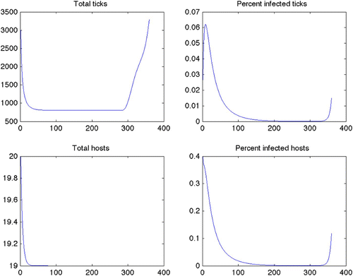
Figure 2. Plots for Scenario 13 (constant grass, quadratic control, maximize disease-free ticks). Top left: total tick population over time. Top right: percent of ticks infected over time. Bottom left: total host population over time (note minimum for Y-axis is 19.0). Bottom right: percent of hosts infected over time. Results from Scenarios 14–24 all produced similar plots.

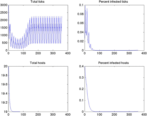
Figure 3. Optimal treatment for Scenario 1 (constant grass, quadratic control, maximize disease free ticks). Note that there is a constant treatment required for nearly the entire length of the scenario. Predicted optimal controls for Scenarios 2–12 produced similar results.

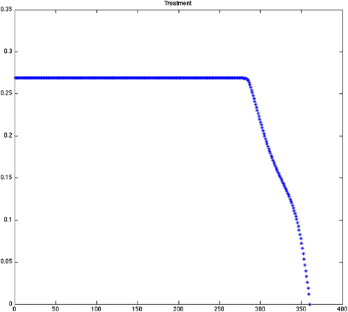
Figure 4. Optimal treatment for Scenario 13 (variable grass, quadratic control, maximize disease-free ticks). Note that after a couple years of constant treatment, the treatment is tapered back to seasonal application and then stopped well before the end of the scenario. Predicted optimal controls for Scenarios 14–24 produced similar results with variation in when constant treatment stopped and when treatment stopped entirely (Table 3).

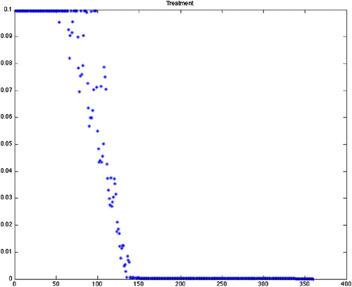
Figure 5. Optimal treatment for Scenario 15 (variable grass, quadratic control, maximize disease-free ticks). This is offered as a comparison between quadratic (Figure 4), mixed and linear (Figure 6) objective functionals. As we mention in Figure 2, the end effect on the tick population is similar.

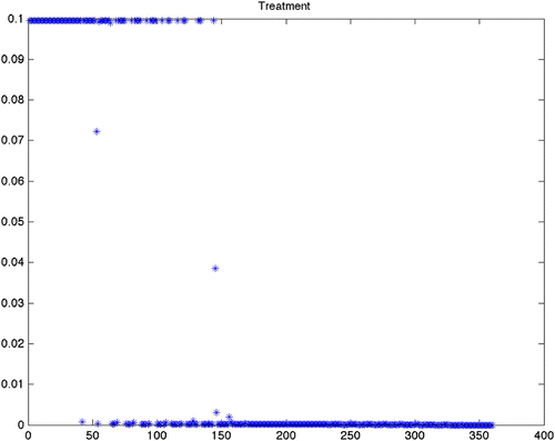
Figure 6. Optimal treatment for Scenario 17 (variable grass, quadratic control, maximize disease-free ticks). This is offered as a comparison between quadratic, mixed and linear objective functionals. As we mention in Figure 2, the end effect on the tick population is similar.

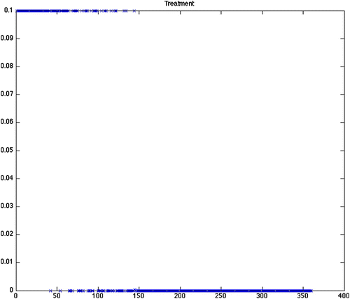
From Table 3, we can see that the predicted optimal control strategy differs greatly between the scenarios using constant birth and death rates (1–12) (Figure 1) and the scenarios using the varying birth and death rates (13–24) (Figure 2). It is important to note that while the results from the varying birth and death rates seem to show chattering, this is simply a reflection of the input parameter variation. The scenarios with constant rates shows that the control efforts will be required to continue at the maximum treatment for an average of more than 26 of the 30-year period. There is little difference with the constant rate scenarios between the grass and wooded habitats. There is also little difference whether using quadratic, mixed or bang-bang control techniques. Finally, there is little difference in the cost of treatment as defined by the sum of effort required for that strategy across all constant rate scenarios (Figures 2–6).

Table 3. Summary results for each scenario.

Scenario	Maximum optimal treatment	Time at maximum	Stop all treatment	Treatment cost
1	0.269 (0.3)	28.916667	29.916667	87.955079
2	0.29 (0.3)	25.666667	25.666667	88.869936
3	0.28 (0.3)	24.916667	24.833333	82.746523
4	0.28 (0.3)	26.416667	26.250000	86.766443
5	0.28 (0.3)	25.000000	24.833333	83.460439
6	0.28 (0.3)	26.583333	26.416667	87.649798
7	0.2675 (0.3)	29.583333	29.916667	88.923389
8	0.28 (0.3)	29.666667	29.916667	94.682668
9	0.28 (0.3)	24.916667	24.833333	83.197294
10	0.28 (0.3)	27.333333	27.333333	91.287848
11	0.28 (0.3)	25.083333	24.916667	83.74412
12	0.28 (0.3)	27.416667	27.250000	91.575036
13	0.1 (0.1)	5.583333	10.916667	10.630587
14	0.1 (0.1)	22.750000	22.833333	25.296268
14a	0.175 (0.175)	12.083333	12.500000	25.296268
15	0.1 (0.1)	3.583333	12.083333	9.317537
16	0.1 (0.1)	22.333333	22.166667	26.612752
16a	0.175 (0.175)	11.583333	12.166667	24.995588
17	0.1 (0.1)	3.583333	12.000000	9.301185
18	0.1 (0.1)	22.333333	22.250000	26.6369
18a	0.175 (0.175)	11.583333	12.166667	24.984107
19	0.1 (0.1)	3.416667	26.000000	12.506637
20	0.1 (0.1)	19.583333	29.333333	31.050363
20a	0.175 (0.175)	12.583333	29.166667	32.28216
21	0.1 (0.1)	3.583333	13.083333	9.451533
22	0.1 (0.1)	20.500000	27.000000	27.994741
22a	0.175 (0.175)	10.583333	17.083333	26.785332
23	0.100000	3.583333	13.083333	9.502303
24	0.100000	20.500000	27.000000	28.001424
24a	0.165000	10.583333	17.166667	26.905953
Notes: For each scenario described in Table 2, a number of metrics are derived from the optimal solution. ‘Maximum optimal treatment’ is the maximum value of the control solution, and the value in parenthesis is the value used for δmax for that scenario. ‘Time at maximum’ is the number of years that the control solution remains at the maximum optimal treatment. ‘Stop all treatment’ is the year when all treatment is stopped out of the 30-year simulation. ‘Treatment cost’ is the projected cost of treatment for the entire 30 years as defined by . Scenario numbers followed by an ‘a’ have the same construct with a different maximum treatment rate.

In contrast, the variable rate scenarios predict control to be needed for as little as 11 years with an average of 13.5 years at maximum treatment. In addition, the level of effort required by the variable rate scenarios is less than half that of the constant rates with similar reductions in the percent of infected ticks. The wooded habitats showed better control in a shorter period of time using an increased maximum treatment rate. The grass habitats (13, 15, 17, 19, 21 and 23) predicted that year-round treatment would only be required for the first 3–5 years followed by another approximately 10 years of seasonal application of maximum control effort. This shortened time frame is reflected in the far smaller costs of the strategies in the grass habitats. This prediction remained consistent across all optimal control techniques and for both objective functionals.

The wooded habitats (14, 16, 18, 20, 22 and 24) predicted approximately 12 years of year-round control with no additional effort in the remaining 18 years. If the wooded habitat is limited to the maximum rate used for the grass habitat, it would take an additional eight or more years of treatment.

3.3. Discussion

This model used six objective functionals to suggest optimal strategies for eradicating tick disease and suggested similar outcomes at a similar cost regardless of the choice of functional. In particular, this suggests that one could give wildlife managers simplified bang-bang advice without loss of results. Secondly, later metapopulation studies can be simplified by not explicitly requiring the preservation of the tick population since the end populations were not sizeably affected by competing strategies.

With constant tick birth and death terms, it is more challenging to control tick disease without eliminating the ticks. The variable birth and death rates reflecting the tick's life history provides a focused time for control efforts. These results highlight the importance of including the tick's life history into a model to assess the potential interventions. This model still has many assumptions that could affect the predictions for the optimal application tick-killing treatment.

Given the differences in the optimal control identified between the grassy and wooded habitats, we will next turn our attention to a spatially explicit, metapopulation optimal control problem. This will allow us to investigate the question of where as well as when and how much tick-killing effort should be used. Additionally, we will need to explore the application of optimal control to models reflecting other tick-borne diseases, such as Lyme disease or Rocky Mountain spotted fever, with more complicated life histories.

The ultimate questions for individuals interested in controlling risk of tick-borne diseases in an area are ‘how long’ and ‘how much’ treatment will be needed to significantly reduce disease risk. The results of this optimal control research indicate that any effort will have to be sustained for many years at an intense level. The results are consistent for all scenarios, but those including the tick life history indicate that this seasonally-fluctuating activity level can be advantageous in minimizing disease risk.

Acknowledgements

The project described was supported by Grant Number K25AI067791 from the National Institute of Allergy and Infectious Diseases. Lenhart's support includes funding from the National Institute for Mathematical and Biological Synthesis (NSF EF-0832858). All authors acknowledge additional support from Grant Number NSF DMS-0813563. The content is solely the responsibility of the authors and does not necessarily represent the official views of the National Institute of Allergy and Infectious Diseases or the National Institutes of Health. K25 Mentoring Committee: J. Stephen Dumler (primary mentor), Abdu Azad, Richard Ostfeld, Daniel Sonenshine and Denise Kirschner.

References

- Blower , S. and Bernoulli , D. 2004 . An attempt at a new analysis of the mortality caused by smallpox and the advantages of inoculation to prevent it . Rev. Med. Virol. , 14 : 275 – 88 .
- Bowman , D. , Little , S. E. , Lorentzen , L. , Shields , J. , Sullivan , M. P. and Carlin , E. P. 2009 . Prevalence and geographic distirbution of Dirofilaria immitis, Borrelia burgdorferi, Ehrlichia Canis, and anaplasma phagocytophilum in dogs in the United States: Results of a national clinic-based serologic survey . Vet. Parasitol. , 160 : 138 – 148 .
- CDC . 2008 . Summary of notifiable diseases – United States, 2006 . Morb. Mortal. Wkly Rep. , 55 : 1 – 94 .
- Coddington , E. A. 1961 . An Introduction to Ordinary Differential Equations , Englewood Cliffs, NJ : Prentice-Hall .
- Coddington , E. A. and Levinson , N. 1955 . Theory of Ordinary Differential Equations , New York : McGraw Hill Co. Inc .
- Ding , W. 2007 . Optimal control on hybrid ODE systems with application to a tick disease model . Math. Biosci. Eng. (SCI) , 4 : 633 – 659 .
- Fister , K. R. , Lenhart , S. and McNally , J. 1998 . Optimizing chemotherapy in an HIV model . Electron. J. Diff. Equ. , 1998 : 1 – 12 .
- Fleming , W. H. and Rishel , R. W. 1975 . Deterministic and Stochastic Optimal Control , Berlin : Applications of Mathematics, No 1 . Springer-Verlag
- Gaff , H. D. and Gross , L. J. 2007 . Modeling tick-borne disease: A metapopulation model . Bull. Math. Biol. , 69 : 265 – 288 .
- Gaff , H. and Schaefer , E. 2010 . “ Metapopulation models in tick-borne disease transmission modeling ” . In Modeling Parasite Transmission and Control, Advances in Experimental Medicine and Biology , Edited by: Michael , E. and Spear , R. C. Vol. 673 , 51 – 65 . New York : Springer . Landes Bioscience
- Gaff , H. and Schaefer , E. 2009 . Optimal control applied to vaccination and treatment strategies for various epidemiological models . Math. Biosci. Eng. , 6 : 469 – 492 .
- Gaff , H. , Gross , L. and Schaefer , E. 2009 . Results from a mathematical model for human monocytic ehrlichiosis . Clin. Microbiol. Infect. Suppl. (S2) , 15 : 15 – 16 .
- Hackbush , W. K. 1978 . A numerical method for solving parabolic equations with opposite orientations . Computing , 20 : 229 – 240 .
- Joshi , H. R. 2002 . Optimal control of an HIV immunology model . Optimal Control Appl. Methods , 23 : 199 – 213 .
- Joshi , H. , Lenhart , S. , Li , M. and Wang , L. 2006 . “ Optimal control methods applied to disease models ” . In Mathematical Studies on Human Disease Dynamics: Emerging Paradigms and Challenges , Edited by: Gumel , A. , Castillo-Chavez , C. , Mickens , R. E. and Clemence , D. P. 187 – 208 . Providence, R.I. : American Mathematical Society .
- Jung , E. , Lenhart , S. and Feng , Z. 2002 . Optimal control of treatments in a two-strain tuberculosis model . Discrete Contin. Dyn. Syst. Ser. B , 2 : 473 – 482 .
- Kamien , M. I. and Schwartz , N. L. 1991 . Advanced Textbooks in Economics , Vol. 31 , Amsterdam : North-Holland Publishing Co .
- Lenhart , S. L. and Workman , J. T. 2007 . Optimal Control Applied to Biological Models , Boca Raton, FL : Chapman Hall/CRC .
- Ostfeld , R. , Price , A. , Hornbostel , V. , Benjamin , M. and Keesing , F. 2006 . Controlling ticks and tick-borne zoonoses with biological and chemical agents . Bioscience , 56 : 383 – 394 .
- Pontryagin , L. S. , Boltyanskii , V. G. , Gamkrelidze , R. V. and Mishchenko , E. F. 1962 . The Mathematical Theory of Optimal Processes , New York, London : Interscience Publishers, John Wiley & Sons .
- Sonenshine , D. E. and Mather , T. N. 1994 . Ecological Dynamics of Tick-Borne Zoonoses , New York : Oxford University Press .