A discrete dispersal model with constant and periodic environments

Abstract

We study a discrete juvenile–adult model which describes the dynamics of a population that reproduces and disperses between two patches constantly or seasonally. When breeding and dispersal rates are constant, the model has a unique interior equilibrium that is globally attractive, provided the net reproductive number is greater than one. If net reproductive number is less than one, then the extinction equilibrium is globally asymptotically stable. When breeding and dispersal rates are periodic of period 2, the extinction equilibrium is globally asymptotically stable if the net reproductive number is less than one. If the net reproductive number is greater than one, then there exists a unique globally attractive periodic solution. We then use bifurcation analysis to compare constant and seasonal breeding strategies, to explore the effects of different birth and dispersal periodicities and to understand the influence of strong nonlinearities on the dynamics of the model.

Keywords:

• population dynamics
• dispersal model
• continuous and seasonal reproduction
• bifurcation analysis

1. Introduction

The process of migration and dispersal has been studied in ecology for many years. Not only has the migration and dispersal of animals, such as birds, insects, and fish, been a popular topic to study, but also the migration and dispersal of plants (seed dispersal) and tissue, blood, and cancer cells are being studied 7 10 11 12 15 20 24. In the last few decades, ecologists and mathematicians have been interested in the dispersal of amphibian populations (4 5 13 16 17 18 22 23 just to name a few).

In the 1960s, Dole studied the summer dispersal of a population of adult leopard frogs, Rana pipiens, in Cheboygan County, Michigan. He was interested in the movements of the adult leopard frogs and the factors controlling them 13. Gibbs examined amphibian movements relative to roads, forest edges, and stream beds by using drift fences and pitfall traps to intercept dispersing amphibians in a forest tract in southern Connecticut. He investigated several amphibian species that were captured, including the pickerel frog, Rana palustris, and the wood frog, Rana sylvatica. Gibbs suggested that the relative permeability of forest-road edges was much reduced compared with the forest interior and with edges between forest and open land 16. From 1995 to 1998, Pilliod et al. researched the habitat use and movement patterns of 736 marked and 87 radio-tagged Columbia spotted frogs, Rana luteiventris, in a mountain basin in central Idaho. Their work showed that many of the Columbia spotted frogs used spatially separated, specific habitat patches for breeding, foraging, and hibernating. They also witnessed that individuals could disperse across hundreds to thousands of metres annually among these complementary resources 22. Kirkland et al. studied general discrete population models where the populations reproduce and disperse in a landscape consisting of a finite number of patches. They wanted to better understand the evolution of dispersal in spatially heterogeneous landscapes by studying the population dynamics for both conditional and unconditional dispersal strategies 19.

We were mainly motivated in this paper by two urban populations of green tree frogs, Hyla cinerea, that are being studied in a joint project by the University of Louisiana at Lafayette and the United States Geological Survey National Wetlands Research Center (USGS NWRC). One population is located at the National Wetlands Research Center/Estuarine Habitat and the Coastal Fisheries Center research complex (referred to as NWRC/EHCFC complex) and the other is located at the Louisiana Immersive Technologies Enterprise Center (referred to as LITE Center). Each location contains man-made ponds with the fringing landscape simulating different wetland types. These populations are relatively isolated as each complex is bordered by buildings, sidewalks, and four lane roads. The distance between the NWRC/EHCFC complex and the LITE Center is approximately half a mile. Dispersal between the ponds is one main topic being studied. For example, in 2008, out of the total number of frogs recaptured at both sites, approximately 1.2% were frogs that had dispersed from one location to the other 21.

In this paper, we develop a juvenile–adult discrete model that describes the dynamics of one species dispersing between two locations, patches 1 and 2. In Section 2, we first analyse the case where the breeding and dispersal rates are constant. Then we study the model by assuming that all the breeding and dispersal rates are seasonal (periodic of period 2). In Section 3, we use bifurcation analysis to compare the population levels resulting from seasonal birth and dispersal rates and constant birth and dispersal rates. We also examine the effects on the population dynamics when considering different periods for the birth and dispersal rates. Finally, we give conclusions in Section 4.

2. Two-stage discrete model

We develop a juvenile–adult discrete model that describes the dynamics of one species dispersing between two locations, patches 1 and 2. We assume that the juveniles and adults only compete with themselves and not with each other. We also assume that the juveniles always remain at their location of birth and only the adults disperse. This is typical of amphibians where the tadpoles remain in the body of water they were born in while the adults move around. Let J _i (t) and A _i (t) denote the number of juveniles and adults, respectively, at time t at patch i for i=1, 2. Let represent the survivorship of the juveniles and represent the survivorship of the adults at time t at patch i for i=1, 2. We will denote the time-dependent birth rates at the two locations as b ₁(t) and b ₂(t). Thus, we obtain the following model:

where m ₁₂(t) is the rate at which adults disperse from patch 1 to patch 2 at time t and where m ₂₁(t) is the rate at which adults disperse from patch 2 to patch 1 at time t. Hence, we assume . Note if m ₁₂=m ₂₁=0, the system (1) reduces to a more general version of the model studied in 3. Also, we assume for the remainder of this paper that and have the following properties:

• (Σ1) For k=J _i , A _i , i=1, 2, , , , and S _k (0)=a _k (0<a _k <1).

Clearly, (Σ 1) is satisfied by the Beverton–Holt dynamics given by , for k=J _i , A _i and also the Ricker dynamics given by , for k=J _i , A _i .

Model (1) will be analysed in two cases. In the first case, we assume b _i (t)=b _i , and are positive constants, while in the second case, we assume b _i (t), m ₁₂(t) and m ₂₁(t) are periodic with period 2.

2.1 Constant birth and dispersion

Consider system (1) with continuous breeding. For the remainder of this section, we assume b _i (t)=b _i , and are positive constant, for i=1, 2. Thus, system (1) can be written as

where , and B has the form

Note that system (1) will always have the trivial steady state . We use the techniques in 9 to find the net reproductive number ℛ₀ of the population. Notice that the inherent projection matrix

where

and

Thus the net reproductive number is the positive strictly dominant eigenvalue of the matrix F(I−G)⁻¹, which is given by

where

Clearly the non-zero eigenvalues of matrix (2) are the eigenvalues of the 2×2 matrix

Let

and

Note that and Therefore, the net reproductive number, in terms of D ₁ and D ₂, is given by

Now, in the following theorem, we provide a stability result for system (1).

Theorem 2.1

Let b _i (t)=b _i , m ₁₂(t)=m ₁₂, and be positive constants, for i=1,2 and t=0, 1, 2…. Assume (Σ 1) holds. If then E ₀ is globally asymptotically stable.

Proof

We will use techniques similar to 2 19. All vector and matrix inequalities hold componentwise. Assume . Define the map to be the right side of system (1). Since B(E ₀) is non-negative, irreducible, and primitive it has a positive, simple, and strictly dominant eigenvalue λ. Since , by [Theorem 1.1.3]8, we know λ<1. Thus, E ₀ is locally asymptotically stable. Let v ^T>0 be the corresponding left eigenvector of λ. That is,

Define as . By (Σ 1), we have that for all X>0. Thus, we have for X>0,

Therefore, as L is a strictly decreasing along the non-zero orbits of P, L(X)=0 if and only if X=0, and L(X)>0 for all X>0, we conclude that Thus, we have that E ₀ is globally asymptotically stable.   ▪

In the following theorem, we show the existence of a unique non-trivial interior steady state for system (1) which is globally attractive. In addition to (Σ 1), we need to assume that and also satisfy

• (Σ2) For k=J _i , A _i , i=1, 2, and .

Note that (Σ 2) is still satisfied by the Beverton–Holt dynamics given by , for k=J _i , A _i . Under (Σ 2), system (1) is monotone. This facilitates the proof of the global attractivity of the interior equilibrium 2 19, which is given in the next theorem.

Theorem 2.2

Let b _i (t)=b _i , m ₁₂(t)=m ₁₂, and be positive constants, for i=1, 2 and t=0, 1, 2…. Assume (Σ 1) and (Σ 2) hold. If then there exists a unique non-trivial interior steady state for system (1) which is globally attractive.

Proof

Assume . Then from the proof of Theorem 2.1, the dominant eigenvalue of B(E ₀), λ, is greater than 1. Define the map to be the right side of system (1). Now we will show that system (1) has a unique interior fixed point X¯. First we will show existence. Let u>0 be the corresponding right eigenvector of λ. That is,

Since B(E ₀)u>u and since B(X) is continuous, there exists ε>0 such that for Y=ε u, we have B(Y)Y≥Y. Note that by (Σ 2), P has the property

Thus, we can conclude that . Hence, P ^t (Y) is an increasing sequence. We know further that P ^t (Y) is bounded from (Σ 2). Therefore as a bounded increasing sequence converges, there exists X¯ such that By the continuity of P, we have . Thus, X¯ is a positive fixed point for P. Next we will show the uniqueness of X¯. First consider the case where 0<X<X¯. Let λ₁ be the positive, simple, and strictly dominant eigenvalue of B(X¯). Since X¯ is a positive fixed point of P, λ₁=1. Let be the corresponding left eigenvector of λ₁ that satisfies . Now, define as Then for 0<X<X¯, we have and

Thus, we have that is a positive increasing sequence that is bounded above by . As L ₁(X)<1 for all X<X¯, we get that for all 0<X<X¯. Similarly, one can show that for all X>X¯. Now for any X>0, we can choose 0<X ₁<X¯ and X ₂>X¯ such that X ₁<X<X ₂. Then P ^t (X ₁ ) < P ^t (X) < P ^t (X ₂ ), for all t>0. But since , it follows from the continuity of P that for all X>0. Therefore, we have that X¯ is the unique, globally attractive positive fixed point.

2.2 Seasonal breeding and dispersion

In this section, we assume that breeding and dispersal movements of the population are seasonal. For example, there are times when the environment is suitable for frogs to hunt, mate, breed, and disperse. And to escape harsh weather, many amphibians including frogs hibernate in winter and estivate when the weather is too hot or dry. During these periods each year, the frogs do not eat, move, or breed. All their life processes drop to a very low level. Hence, we assume in model (1) that the dispersal rates m ₁₂(t), m ₂₁(t) and the birth rates b _i (t), i=1, 2 are periodic with period 2. Specifically, we let for i=1, 2, and we take , where . In other words, if the time unit is half a year and a full cycle consists of one year, the population gives birth and disperses only half the year, while in the other half there is no dispersal or birth.

We will find the net reproductive number for the seasonal breeding case by using similar techniques used in the continuous breeding case. From 6 14, since system (1) is periodic with period 2, we define the projection matrix over a full cycle [Bcirc](X) to be the product of the following matrices, where the short notation S _k represents S _k (k), for k=J _i , A _i , and i=1, 2.

Thus, the resulting product matrix is

Note the inherent projection matrix over a full cycle is

where

and

Therefore, the net reproductive number is the positive, strictly dominant eigenvalue of . After some calculations, we obtain

where

Notice that non-zero eigenvalues of Equation (4) are the eigenvalues of the 2×2 matrix

Let

and

Again, note that and Thus, the net reproductive number, in terms of [Dcirc] ₁ and [Dcirc] ₂, is given by

The following theorem shows the global stability of the extinction equilibrium E ₀.

Theorem 2.3

For t=0, 1, 2, …, and for i=1, 2, let and where . Assume (Σ 1) holds. If then is globally asymptotically stable.

Proof

Let and (Σ 1) hold. Define the map to be the right side of Equation (1). Since , by [Theorem 1.1.3, p. 10]8, we have that the dominant positive eigenvalue, λˆ, of the non-negative, irreducible, and primitive matrix [Bcirc](E ₀) is also less than one. So E ₀ is locally asymptotically stable. From (Σ 1), system (1) has the property

where the vector and matrix inequalities hold componentwise. Thus, for X>0, we have

Since , then . Therefore, for any X(0)>0, we have

and

Since both and converge to 0 as t→∞, the solution converges to 0. Thus, E ₀ is globally asymptotically stable.   ▪

In the following theorem, we show the existence of a unique non-trivial two-cycle for system (1) which is globally attractive in . To prove global attractivity, we again require that the assumptions in (Σ 2) hold in order for the system to be monotone.

Theorem 2.4

For t=0, 1, 2, …, and for i=1, 2, let and where . Assume (Σ 1) and (Σ 2) hold. If then there exists a unique non-trivial two-cycle for system (1) which is globally attractive in .

Proof

Suppose (Σ 1) and (Σ 2) hold and that . We will use techniques akin to 1. We see that

as b _i (2t)=0, for i=1, 2, and

as . From this, we get

and

where

and

  ▪

Let for i≥0. Then we have the following system

Here,

and

We can write system (6) as

where and [Btilde] has the form

where

Therefore, the inherent projection matrix of system (6) is given by

Now by assumption, . So it follows that the spectral radius of , λˆ, is greater than one. Let to be the right-hand side of Equation (6). It can be easily shown that the Jacobian matrix for all X≥0 by (Σ2). Thus, [Ptilde](X) is monotone.

Then by a similar argument as in the proof of Theorem 2.3, we can show that system (6) has a unique interior fixed point , which is globally attractive. Thus, we have that

It follows that

Hence, Equation (1) has a unique, globally attractive 2-cycle.

3. Bifurcation analysis

In Section 3.1, we address the question of whether a seasonal breeding strategy is advantageous or deleterious over a constant breeding strategy. In Section 3.2, using bifurcation analysis, we study our model with birth and dispersal rates that are periodic with periods 3 and 6. We compare these results with the period 2 case studied in Section 2. Then, in Section 3.3, we replace the Beverton–Holt non-linearities with Ricker-type non-linearities to study the effects of strong non-linearities on the dynamics of the population.

3.1 Period 2 versus constant birth rate

We are interested in understanding whether there are birth rates b for which seasonal breeding is advantageous over constant breeding. In particular, are there values of b in which a seasonal breeding strategy will result in an average adult population size that is larger than with a constant breeding strategy? To compare on an equal basis, we assume that over a complete cycle (composed of p time units), an adult produces the same number of juveniles whether breeding constantly or seasonally. For period 2, the constant breeders will produce b+b=2b offspring in one complete cycle. The seasonal breeders will produce offspring in one complete cycle. Therefore, we assume that [bcirc]=2 b. In the same light, we take and . In the following example, we show that for low birth rates the periodic strategy has an average adult population that is larger than that of the constant. While for large birth rates, the opposite happens.

For this example, we assume that the environment in patch 2 is better than that in patch 1. Therefore, we assume that the birth rate in patch 2 to be higher than that in patch 1, the dispersal rate from patch 1 to patch 2 is higher than that from patch 2 to patch 1, and the survivorship rate in patch 2 is higher than that in patch 1. In particular, we use , , , and where , and . We set b ₁=b, b ₂=b+1, m ₁₂=0.04, and m ₂₁=0.01. 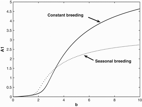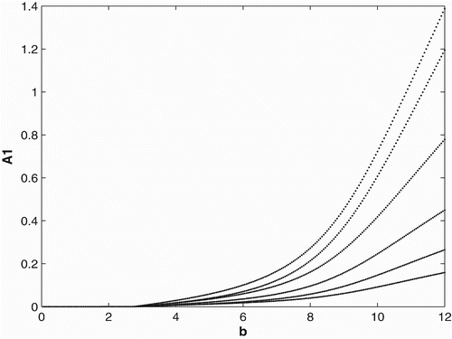The initial conditions are , A ₁(0)=4, and A ₂(0)=5. A similar scenario seems to occur at the two locations of our motivating populations of green tree frogs. Among all the recaptures of green tree frogs in 2008, there were four times as many frogs migrating to the NWRC/EHCFC complex than to the LITE Center. In Figure 1, we provide a bifurcation diagram for the constant and seasonal birth and migration rates with the birth rate used as a bifurcation parameter. This example shows that for birth rates less than ∼0.07, both populations with a seasonal breeding and constant breeding strategy will become extinct. We also can see that for birth rates both the constant and seasonal breeders will survive, but seasonal breeding is advantageous over constant breeding. For birth rates b>3.36, we see that constant breeding is advantageous.

Figure 1. Bifurcation diagrams for the continuous and seasonal birth rate. The bifurcation diagram of the seasonal case is the cycle average of the adult population in patch 1.

3.2 Constant and periodic breeding and dispersal rates

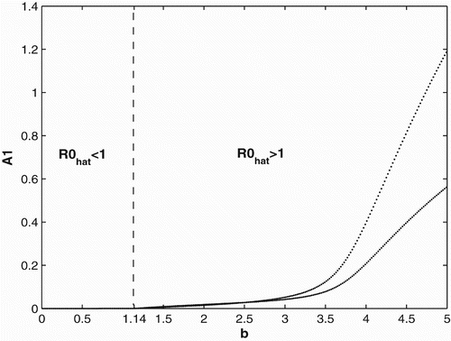
We first provide bifurcation diagrams illustrating our theoretical conclusions in Section 2. In Figures 2 and 3, we graph the population of adults in patch 1. The bifurcation diagram of the other adult population and the juveniles are similar and hence are not presented. We use the same survivorship functions and parameter values as in Section 3.1. Figure 2 is the bifurcation diagram for constant breeding and dispersal. For b<0.35, the population becomes extinct, while the population persists for b>0.35. Figure 3 is the bifurcation diagram for the period 2 birth and dispersal rates of the form used in Section 2. Extinction of the population occurs for b<1.14, while for b>1.14, the population persist and converges to a two-cycle.

Figure 2. Bifurcation diagram for the continuous birth and dispersal rates.

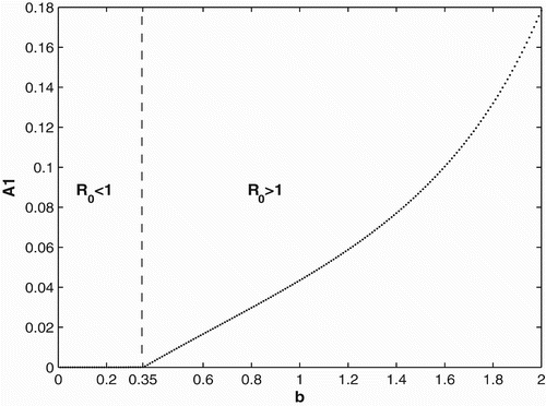
Figure 3. Bifurcation diagram for the seasonal birth and dispersal rates of period 2.

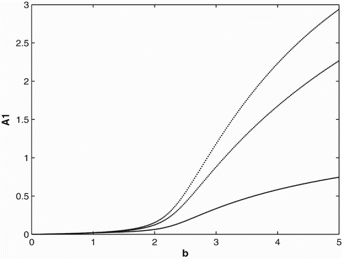
In Figure 4, we set a ₁=0.5, a ₂=0.4, a ₃=a ₄=0.6, . We consider period 3 birth rates of the form , and period 3 dispersal rates of the form and . In other words, if a full cycle is a year (composed of three time units, 4 months each), the populations would breed and disperse for only 8 months out of the year. We can see that when the birth rate gets large enough, the population persists and converges to three cycles.

Figure 4. Bifurcation diagram for the seasonal birth and dispersal rates of period 3.

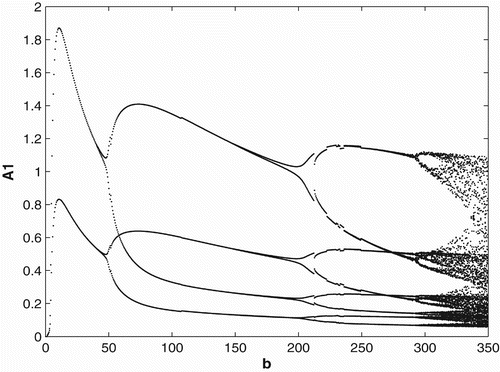
Next we consider the case where birth rates are period 6 of the form , and dispersal rates are period 6 of the form and . This strategy suggests that dispersal begins before and ends after the breeding season. In this example, we let a ₁=0.4, a ₂=0.6, a ₃=0.5, a ₄=0.7, . Figure 5 shows that when the birth rate gets large enough, the population persists and converges to six cycles.

Figure 5. Bifurcation diagram for the seasonal birth and dispersal rates of period 6.

3.3 Ricker-type non-linearities

In order to study the effects of survivorship functions that are strong non-linearities as opposed to weak non-linearities, we replace the Beverton–Holt non-linearities in our model used in Sections 3.1 and 3.2 with Ricker-type non-linearities. In Figure 6, we consider Ricker-type survivorship functions with constant birth and dispersal rates, and in Figure 7, we consider seasonal birth and dispersal rates of period 2. We use the following Ricker-type survivorship functions , , , . The parameter values and initial conditions are set to be the same as in Section 3.1. We see that the Ricker-type survivorship functions result in much richer dynamics than those with the Beverton–Holt functions used in Section 3.2, including chaotic dynamics. Observe, however, that in comparison with the constant case, seasonal birth and dispersal rates tend to stabilize the population dynamics. In particular, for some values of birth rates when the population has chaotic dynamics in the constant rate strategy, it has periodic dynamics under the seasonal rate strategy.

Figure 6. Bifurcation diagram for the continuous birth and dispersal rates with Ricker-type survivorship functions.

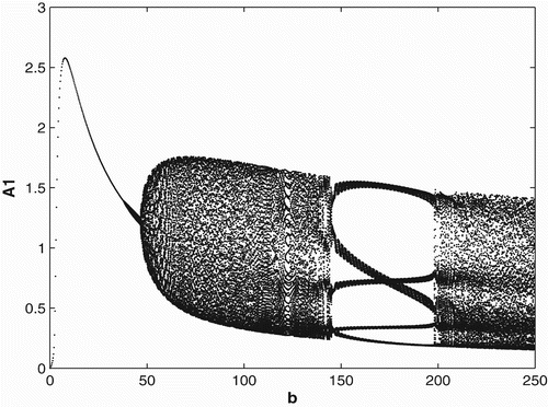
Figure 7. Bifurcation diagram for the seasonal birth and dispersal rates of period 2 with Ricker-type survivorship functions.

4. Conclusion

In this paper we develop and analyse a discrete juvenile–adult model (1) with constant or seasonal reproduction and dispersion. When the population breeds and disperses with constant rates b _i , i=1,2, and m ₁₂, m ₂₁, respectively, we show that when the net reproductive number the extinction equilibrium E ₀ is globally asymptotically stable; while if , the model has a unique interior equilibrium which is globally attracting. When assuming the population breeds and disperses periodically with period 2, we get that if , then the extinction equilibrium E ₀ will be globally asymptotically stable. If , then the model has a unique non-trivial periodic solution, which is globally attractive.

Bifurcation diagrams conclude that for low birth rates, the periodic strategy has an average adult population that is larger than that of the constant, while for large birth rates, the opposite happens. This indicate that seasonal breeding is advantageous for low birth rates and deleterious for high birth rates.

Finally, we consider the notion of using weak non-linearities as opposed to strong non-linearities for the survivorship functions in our models. In Section 3.2, we demonstrated bifurcation diagrams for Beverton–Holt non-linearities. The results indicate the existence of a periodic solution which emanates from the periodic environment. When replacing the Beverton–Holt non-linearities with Ricker-type non-linearities, the dynamics become much richer including chaotic dynamics. The data collected from 2004 to 2009 on our motivating population of green tree frogs indicates that the population oscillates and the length of the oscillation is 1 year. This suggests that weak non-linearities are likely to describe the type of competition occurring in this population and the fact that oscillation in this population arises from seasonality.

Acknowledgements

The work of A.S. Ackleh and P. Zhang was supported in part by the National Science Foundation under grant # DUE-0531915. The work of A.S. Ackleh was also supported in part by the National Science Foundation under grant # DMS-0718465. We would like to thank Dan Sutton and Tracey Robin for their participation in the summer research project related to the work in this paper. We would also like to thank the referees for their useful comments and suggestions.

References

- Ackleh , A. S. and Chiquet , R. A. 2009 . The global dynamics of a discrete juvenile-adult model with continuous and seasonal reproduction . J. Biol. Dyn. , 3 : 101 – 115 .
- Ackleh , A. S. and De Leenheer , P. 2008 . Discrete three-stage population model: Persistence and global stability results . J. Biol. Dyn. , 2 : 415 – 427 .
- Ackleh , A. S. and Jang , S. R.-J. 2007 . A discrete two-stage population model: Continuous versus seasonal reproduction . J. Diff. Equ. Appl. , 13 : 261 – 274 .
- Blaustein , A. R. , Wake , D. B. and Sousa , W. P. 1994 . Amphibian declines: Judging stability, persistence, and susceptibility of populations to local and global extinctions . Conserv. Biol. , 8 : 60 – 71 .
- Carr , L. W. and Fahrig , L. 2001 . Effect of road traffic on two amphibian species of differing vagility . Conserv. Biol. , 15 : 1071 – 1078 .
- Caswell , H. 2001 . Matrix Population Models , 2 , Sunderland : Sinauer .
- Cox , G. W. 1985 . The evolution of avian migration systems between temperate and tropical regions of the new world . Amer. Nat. , 126 : 451 – 474 .
- Cushing , J. M. 1998 . “ An Introduction to Structured Population Dynamics ” . Philadelphia : SIAM .
- Cushing , J. M. and Yicang , Z. 1994 . The net reporductive value and stability in matrix population models . Nat. Res. Model. , 8 : 297 – 333 .
- DiMilla , P. , Barbee , K. and Lauffenburger , D. A. 1991 . Mathematical model for the effects of adhesion and mechanics on cell migration speed . Biophys. J. , 60 : 15 – 37 .
- DiMilla , P. , Stone , J. A. , Quinn , J. A. , Albelda , S. M. and Lauffenburger , D. A. 1993 . Maximal migration of human smooth muscle cells on fibronectin and type IV collagen occurs at an intermediate attachment strength . J. Cell Biol. , 122 : 729 – 737 .
- Dingle , H. 1982 . Function of migration in the seasonal synchronization of insects . Entomol. Exp. Appl. , 31 : 36 – 48 .
- Dole , J. W. 1965 . Summer movements of adult leopard frogs, Rana Pipiens Schreber, in northern Michigan . Ecology , 46 : 236 – 255 .
- Elaydi , S. 2005 . An Introduction to Difference Equations , 3 , New York : Springer .
- Elzer , K. L. , Heitzman , D. A. , Chernin , M. I. and Novak , J. F. 2008 . Differential effects of serine proteases on the migration of normal and tumor cells: Implications for tumor microenvironment . Integr. Cancer Ther. , 7 : 282 – 294 .
- Gibbs , J. P. 1998 . Amphibian movements in response to forest edges, roads, and streambeds in Southern New England . J. Wildl. Manage. , 62 : 584 – 589 .
- Grayson , K. L. and Wilbur , H. M. 2009 . Sex- and context-dependent migration in a pond-breeding amphibian . Ecology , 90 : 306 – 312 .
- Halley , J. M. , Oldham , R. S. and Arntzen , J. W. 1996 . Predicting the persistence of amphibian populations with the help of a spatial model . J. Appl. Ecol. , 33 : 455 – 470 .
- Kirkland , S. , Li , C. and Schreiber , S. J. 2006 . On the evolution of dispersal in patchy landscapes . SIAM J. Appl. Math. , 66 : 1366 – 1382 .
- Levey , D. J. and Stiles , F. G. 1992 . Evolutionary precursors of long-distance migration: Resource availability and movement patterns in neotropical landbirds . Am. Nat. , 140 : 447 – 476 .
- Pham , L. , Boudreaux , S. , Karhbet , S. , Price , B. , Ackleh , A. S. , Carter , J. and Pal , N. 2007 . Population estimates of Hyla Cinerea (Schneider)(green tree frog) in an urban environment . Southeast. Nat. , 6 : 203 – 216 .
- Pilliod , D. S. , Peterson , C. R. and Ritson , P. I. 2002 . Seasonal migration of Columbia spotted frogs Rana luteiventris among complementary resources in a high mountain basin . Can. J. Zool. , 80 : 1849 – 1862 .
- Pope , S. E. , Fahrig , L. and Gray Merriam , H. 2000 . Landscape omplementation and metapopulation effects on leopard frog populations . Ecology , 81 : 2498 – 2508 .
- Roff , D. A. 1986 . The evolution of wing dimorphism in insects . Evolution , 40 : 1009 – 1020 .