Complex behaviour in four species food-web model

Abstract

A four-dimensional food-web system consisting of a bottom prey, two middle predators and a generalist predator has been developed with modified functional response. The system is well posed and dissipative. Some results on uniform persistence have been developed. The dynamics of the system is found to be chaotic for certain choice of parameters. The coexistence of all four species is possible in the form of periodic orbits/strange attractors for suitably chosen set of parameters.

Keywords:

• dissipative
• stability
• uniform persistence and chaotic behaviour

AMS Subject Classification:

• Primary: 92B05, 92D25, 37N25
• Secondary: 70K05, 37D45

1. Introduction

Communities or ecosystems with one or two species are very rare in nature. Coexistence of a large number of species is almost universal in natural communities and ecosystems 20. Over the last three decades, many mathematical models have been investigated to study the dynamics of three interacting species in food chains/webs. Few models for more than three species also exist 26. These studies indicate the complexity in the dynamics of such systems. The coexistence of species may not be only in terms of stability of singularities and orbits, it may happen in more complex forms such as quasi-periodic or strange attractors 17.

Many simulation studies have shown that food chain models can have chaotic dynamics, generally obtained through a cascade of period doubling 1 17 18 21–24 27. Hastings and Powell 17 demonstrated the existence of a ‘tea-cup’ strange attractor in a three-trophic-level food chain. McCann and Yodzis 21 pointed out that parameters used to obtained the strange attractor by many of the investigators may not be biologically feasible. However, parameters used by Scheffer 24 for plankton and by Wilder et al. 27 for a study of gypsy moths are biologically feasible. This fact, together with the analysis carried out by Abrams and Roth 1 and by McCann and Yodzis 21 22 on food chains and food webs might, indeed, be those of a strange attractor. The above results justify the interest for a deeper understanding of the complexity of food chains/webs.

El-Owaidy and Ammar 6 investigated a three-level food web. The food web consists of a prey at the lowest level, a specialist predator at the second level and another generalist predator at the highest level. The model deals with the dynamics around the stability of various isolated singularities, but it raises certain doubts about various functional responses in the model. The functional response of one prey species is independent of the density of other prey species, that is, the predator takes food from a prey species irrespective of the food that has already been taken from another prey species. It appears that the predator has two guts, one for each prey species. The model is rectified by modifying the functional response by Gakkhar and Naji 13. Through numerical simulations they had shown the existence of chaos in the model for biologically feasible parametric values. The presence of chaotic nature in three species food chain/web models has also been established in 12 15.

El-Owaidy et al. 7 investigated a four-level generalized food chain model. However, this model also suffers from the same problem as in 6. The authors analysed the existence of a bounded solution and investigated the stability of various equilibrium points. However, the complex dynamics of the model was not explored.

The paper is organized as follows. In Section 2, model formulation using various functional responses has been shown. The explicit conditions for Kolmogorov subsystems have been obtained in Section 3. The system has been proved to be dissipative in Section 2. The local behaviour of the various singularities has been discussed in Section 5. The uniform persistence of three-dimensional subsystems has also been discussed. The uniform persistence of a four-dimensional system is analysed in Section 6. Extensive numerical simulations are carried out in Section 7 to support the analytical results and to explore the complex dynamics of the system. The paper ends with a discussion.

2. Model formulation

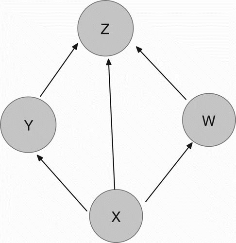
Consider a food web comprising of four species and three trophic levels. This food web consists of a bottom prey with density X, two middle predators with densities Y and W feeding on the bottom prey and a top predator with density Z feeding on all three other populations. There is no explicit interaction between two middle predators as shown in Figure 1. The dynamics of four species are governed by the following system:

The following assumptions are made on growth and interaction functions:

A1. The bottom prey is growing logistically g(X)=a ₀(1−X/K) such that

A2. The Holling type-II functional response of the middle predators to prey X are

A3. Since top predator takes food from all three (a bottom prey and two middle predators), the functional responses are assumed, respectively, as

The following non-dimensional variables and constants are introduced:

Accordingly, system (1) is transformed to the following non-dimensional vector field :

In system (2), all the model parameters are positive and have usual meanings in the ecological context. The system is associated with the initial conditions:

Figure 1. Energy flow diagram of the model.

3. Kolmogorov analysis

The food-web system is feasible if it is possible to split the system into feasible prey–predator subsystems in the absence of other predators 5. Accordingly, only three subsystems are possible, namely x y, x z and x w. Three biologically feasible two-dimensional subsystems are now formulated from system (2)

These Kolmogorov subsystems are biologically feasible in x y-plane, x w-plane and x z-plane, respectively 8, under the following respective conditions:

Further analysis of system (2) is carried out under conditions (6)–(8).

4. Analysis of the system

It is observed that all the interaction functions involved in system (2) are continuous and have continuous derivatives on the non-negative orthant

Therefore, system (2) admits a unique solution in . If the prey species is resource limited, then all predator species are also be limited regardless of their predation curves. Accordingly, the solution of the system initiating in the first orthant must be bounded. Further, a biologically feasible model must be dissipative, that is, all populations are uniformly limited in time by their environments 9.

Theorem 4.1

The solution of system ( 2) initiating in is uniformly bounded. Moreover, the system is dissipative in .

Proof

The system (2) is dissipative in , if solutions (x(t), y(t), w(t), z(t)) of the system initiating in it are uniformly bounded as .

From the first equation of system (2),

Standard comparison theorem on differential equations gives

Let A ₁(t)=x(t)+y(t)/w ₄. Computing and simplifying its derivatives give

Similarly, introducing A ₂(t)=x(t)+w(t)/w ₁₄ gives

Let

Then,

Thus, all the solutions of system (2) enter into the region

Here, B ₀ is a connected compact set and an invariant attractor for the flow of the system. Therefore, system (2) is uniformly bounded. Hence, it is dissipative.

5. Local behaviour of the system

In this section, the local behaviours of isolated singularities of system (2) are investigated and the results are stated in the form of theorems.

Theorem 5.1

1.	The trivial singularity E 0 =(0, 0, 0, 0) of system ( 2) always exists. It is hyperbolic saddle having one-dimensional unstable manifold W u (E 0) along the x-direction.
2.	The axial singularity E 1 =(1, 0, 0, 0) always exists. It is hyperbolic saddle having one-dimensional stable manifold W s (E 1) along the x-direction.

The results are evident from the eigenvalues of the associated variational matrix.

5.1. Behaviour of the system in a two-dimensional hyperplane

For the Kolmogorov system, a unique singularity always exists in the hyperplane .

The local behaviour of the singularity E ₂ is given in the following theorem.

Theorem 5.2

1.	The singularity E 2 is a hyperbolic attracting focus in the hyperplane Ω 1 provided:
2.	The singularity E 2 has an invariant hyperbolic repelling manifold in the w-direction when n 2 >0. Similarly,  it has an invariant hyperbolic repelling manifold in the z-direction when n 3 >0.
3.	There exists a small neighbourhood of n 1 =0 such that the singularity E 2 has a supercritical Andronov–Hopf bifurcation in the hyperplane Ω 1 ,  bifurcating to a hyperbolic attracting limit cycle.

Proof

Consider the variational matrix:

Parts (1) and (2) of Theorem 5.2 are evident from the eigenvalues of the matrix D X _η(E ₂).

It is observed that the sum of eigenvalues in the x y-plane is equal to zero when n ₁=0. This is possible only when w ₁>1. Accordingly, the first Liapunov exponent L ₁, at singularity E ₂ is zero 2 3. The second Liapunov exponent is computed as

Since E ₂ is attracting focus when n ₁<0 and repelling when n ₁>0, the system undergoes supercritical Andronov–Hopf bifurcation and bifurcates to a limit cycle. Moreover, since L ₂ is negative, it is an attracting limit cycle. This proves Part (3) of Theorem 5.2.

For the Kolmogorov system (2), there always exists a unique singularity in the hyperplane .

Also, in the hyperplane , there always exists a unique singularity .

Proceeding on similar lines, as above, the local behaviours around E ₃ and around E ₄ are stated in the next theorems (proofs omitted):

Theorem 5.3

1.	The singularity E 3 is a hyperbolic attracting focus in the hyperplane Ω 2 provided:
2.	The singularity E 3 has an invariant hyperbolic repelling manifold in the y-direction if n′ 2 >0. Similarly,  it has an invariant hyperbolic repelling manifold in the z-direction when n′ 3 >0.
3.	There exists a small neighbourhood of n′ 1 =0 such that the singularity E 3 has a supercritical Andronov–Hopf bifurcation in the hyperplane Ω 2 ,  bifurcating to a hyperbolic attracting limit cycle.

Theorem 5.4

1.	The singularity E 4 is a hyperbolic attracting focus in the hyperplane Ω 3 provided:
2.	The singularity E 4 of the system has an invariant hyperbolic repelling manifold in the y-direction if n′′ 2 >0. Similarly,  it has an invariant hyperbolic repelling manifold in the w-direction when n′′ 3 >0.
3.	There exists a small neighbourhood of n′′ 1 =0 such that the singularity E 4 has a supercritical Andronov–Hopf bifurcation in the hyperplane Ω 3 ,  bifurcating to a hyperbolic attracting limit cycle.

5.2. Behaviour of three-dimensional subsystems

In the absence of a middle predator w, the subsystem X _η(x, y, 0, z) exists in hyperspace . The conditions for persistence of the subsystem is investigated in the following section.

Theorem 5.5

If n ₃ >0 and n′′ ₂ >0,  then the three-dimensional subsystem X _η(x, y, 0, z) is uniformly persistent when one of the following set of conditions is satisfied.

a.	[In the absence of periodic solutions in xy- and xz-planes] n 1 <0,  n′′ 1 <0.
b.	[In the absence of periodic solutions in the xz-plane] n′′ 1 <0 and for each periodic solution of period τ 1 in xy-plane.
c.	[In the absence of periodic solutions in the xy-plane] n 1 <0 and for each periodic solution of period τ 2 in xz-plane.
d.	[In the presence of periodic solutions in both xy- and xz-planes] and for each periodic solution of period τ 1 in the xy-plane and for each periodic solution of period τ 2 in the xz-plane.

Proof

By Theorem 5.2, there exists a hyperbolic repelling manifold in an orthogonal direction to the x y-plane when n ₃>0. The condition n′′₂>0 implies that there exists a hyperbolic repelling manifold in an orthogonal direction to the x z-plane.

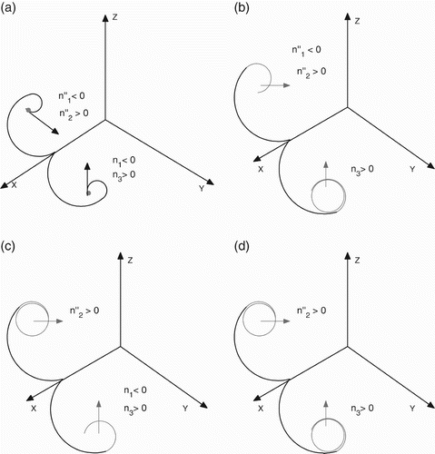
a.	Clearly, under condition (a) of Theorem 5.5, the subsystem X η(x, y, 0, z) will not admit any periodic solutions in boundary planes (Figure 2(a)). In this case, the proof of Theorem 5.5 is obvious 11.
b.	In this case, the subsystem X η(x, y, 0, z) will not admit periodic solutions in the x z-boundary plane when n′′1<0. However, the x y-boundary plane may have periodic solutions (Figure 2(b)). Let O(X) be the orbit through the interior point X=(x, y, 0, z) and Ω(X) be the ω-limit set of O(X). Note that Ω(X) is bounded. Using Butler–McGehee lemma 11, it is observed that E 0, E 1 and E 3 does not belong to Ω(X). Now, we show that no periodic orbits in the x y-plane or E 2 belongs to Ω(X). Suppose γ i ,  i=1, 2, …, n denotes the closed orbit of the periodic solution in the x y-plane such that γ i lies inside γ i−1. The variational matrix corresponding to γ i is obtained as The fundamental matrix of the linear periodic system is computed as The floquet multiplier in the z-direction is . Proceeding along the lines of Kumar and Freedman 19, it is concluded that no γ i lies in Ω(X). Thus, Ω(X) lies in the positive octant. Hence, the system X η(x, y, 0, z) is persistent. The dissipative nature of the system leads to uniform persistence of the subsystem X η(x, y, 0, z) in this case 4 10.
c.	Also, under these conditions, the subsystem X η(x, y, 0, z) admits periodic solutions in the x z-boundary plane only (Figure 2(c)). In this case, the proof of this part is similar to the previous one.
d.	The subsystem X η(x, y, 0, z) admits periodic solutions in both boundary planes x y and x z (Figure 2(d)). The proof is similar.

Figure 2. Dynamics of the three-dimensional subsystem in the absence of the middle predator w. (a) No periodic solutions in x y- and x z-planes; (b) no periodic solutions in the x z-plane, but periodic solution in the x y-plane; (b) no periodic solutions in the x y-plane, but periodic solution in the x z-plane and (c) periodic solutions in both x y- and x z-planes.

The solution of the system of equations gives the non-trivial singularity in the space , where and are uniquely expressed in terms of , while is obtained from the quadratic:

Accordingly, the vector field X _η(x, y, 0, z) under Kolmogorov conditions admits unique singularity when

The vector field X _η(x, y, 0, z) has two singularities when

The application of the Routh–Hurwitz criterion gave rise to intractable mathematical conditions for the local stability of E ₅.

Let us assume that the unique singularity of the vector field X _η(x, y, 0, z) has an index of stability one (i.e. has stable manifold in only one direction). The following gives the conditions for existence of an invariant compact set in Ω₄.

Theorem 5.6

For the vector field X _η(x, y, 0, z) having unique singularity in the interior of Ω ₄ with an index of stability one,  there exists an attracting compact set in its interior provided:

Proof

Let be the flow of the vector field X _η. By Theorem 4.1, the vector field X _η(x, y, w, z) is bounded in and implies that the subsystem X _η(x, y, 0, z) is also bounded in a positive octant Ω₄.

By Theorem 5.1, the singularities E ₀ and E ₁ are hyperbolic saddle points. Moreover, under conditions (11), there are no periodic orbits in x y- and x z-planes but the singularity E ₂ has a repelling manifold along the z-direction and singularity E ₄ has a repelling manifold along the y-direction pointing towards the interior of Ω₄. Clearly, these singularities are not the ω-l i m i t s of the orbits initiating in the interior of Ω₄.

Now, if in the interior of Ω₄, there exists only one singularity E ₅ having an index of stability one, then there must exist a connected compact set (‘trapping region’), which contains neither any singularities nor the tubular neighbourhood of stable manifold W ^s (E ₅) of E ₅, such that the flow Φ(t) crosses its frontier ∂Σ transversally towards the interior of Σ. The associated attracting set (maximal invariant set) is given as

By definition 16, Γ is non-empty because it is an intersection of decreasing family of compact sets. Moreover, it is an invariant maximal attracting set in Σ. Furthermore, it is not difficult to see that Γ is a path-connected set and does not reduce to a single point since the only singularity (E ₅ has stable manifold in one direction only). Therefore, there exists an invariant compact set , which contains all possible orbits of X _η(x, y, 0, z). This proves Theorem 5.6.

Remark 1

i.	With this attracting invariant compact set, the coexistence of three species with time is guaranteed. Observe that the orbits initiating in complement of the tubular neighbourhood of the stable manifold of E 5 in the interior of Ω4 tends to the attractor Λ1. This ensures the coexistence of three species in time.
ii.	Although the singularity E 5 is assumed to be of the index of stability one in Theorem 5.6, no explicit conditions could be derived for the same. Further, under certain choice of parameters (condition (10)), it is possible to have more than one singularity of the vector field X η(x, y, 0, z). It is expected that one of them may be a saddle.
iii.	Results similar to Theorems 5.5 and 5.6 are obtained for the other subsystem X η(x, 0, w, z) in the absence of predator y.

6. Analysis of the system in four dimensions

When no periodic orbits are possible in the coordinate planes x y, x w and x z of the proposed system X _η(x, y, w, z), the conditions for persistence are obtained in the following theorem.

Theorem 6.1

The system X _η(x, y, w, z) is uniformly persistent when one of the following set of conditions holds:

Proof

By Theorem 4.1, the system X _η(x, y, w, z) is uniformly bounded and dissipative. Clearly, under conditions (6)–(8), the system X _η(x, y, w, z) has unique singularities in coordinate planes x y, x w and x z. Moreover, there are no equilibria in y z- and w z-planes.

From Theorem 5.2, it is clear that no periodic solution exists in x y-plane and it has a repelling manifold along the z-direction (under first condition of Equation (13)).

Accordingly, any solution initiating in the neighbourhood of the x y-plane will be attracted by the x z-plane. Now, the x z-plane has no periodic solutions and has repelling manifolds along w-direction (second condition of Equation (13), Theorem 5.4).

Due to the third condition of Equation (13), there are no periodic orbits and the inward trajectories in x w-plane will be repelled again towards the x y-plane (Theorem 5.3).

Hence, all the four species coexist in the interior of . Further, dissipative nature of the system guarantees the uniform persistence of the system X _η(x, y, w, z).

Similar argument gives uniform persistence in the case of the set of condition (14) also. (This proof is inline with the proof of Theorem (3.1) in 11, where conditions of persistence have been satisfied.)

Remark 2

It is realized that Theorem 6.1 regarding the persistence of system (2) is of limited applicability. In the case of periodic solutions existing in boundary planes and in three-dimensional hyperspace, no such criteria have been established.

A unique non-zero singularity E ₇=(x*, y*, w*, z*) of the vector field X _η(x, y, w, z) in Ω is obtained under the condition:

Two singularities of X _η(x, y, w, z) are obtained, when

Local stability of E ₇ can be analysed using Routh–Hurwitz criterion. However, the complex and intractable conditions so obtained could not yield any meaningful result.

In the absence of any such analytical results, numerical simulations are carried out to investigate the complex dynamics and coexistence of four species of the system.

7. Numerical simulations

To verify the analytical results and explore the global dynamics of four species food-web model, extensive numerical simulations are carried out. The system is numerically solved for suitable combination of parameter values. The parameters are chosen in such a manner that Kolmogorov conditions (6)–(8) are satisfied. Since bifurcation diagrams are considered as a tool for locating and identifying the signatures of chaos in a system, they are drawn with respect to critical parameters in a specific range. Attractors of the vector field X _η(x, y, w, z) in Ω are also drawn at selected values of the critical parameters, for example, an attractor in four dimensions is depicted in x y z- and x w z-phase space plots. Time series are also drawn in some cases to show the extinction or coexistence in the four species food-web model.

Consider the following set of data for the vector field X _η(x, y, 0, z):

For the data set (17), the singularity E ₂=(0.206186, 1.02296, 0, 0) is an attracting focus in x y-plane and has an unstable manifold along the z-axis. The singularity E ₄=(0.57193, 0, 0, 1.6522) is also an attracting focus in the x z-plane and has an unstable manifold along the y-axis. Thus, E ₂ and E ₄ have one-dimensional unstable manifolds in axial directions. The three-dimensional subsystem X _η(x, y, 0, z) is uniformly persistent in this case. Further, E ₅=(x=0.319781, y=0.103251, w=0, z=2.08542) is the only singularity in the interior of Ω₄ since . The eigenvalues associated with singularity E ₅ is given by (λ _x =0.060983+0.120909i, λ _y =0.060983−0.120909i, λ _z =−0.120744). The existence of non-trivial invariant attracting compact set in the interior of Ω₄ is now possible due to Theorem 5.6. This implies that, the prey and both the predators coexist in time which tends to the maximal invariant set Λ₁ proved in Theorem 5.6. The bifurcation diagram with respect to w ₂ in the range (3.5–5.5) is drawn in Figure 3. The existence of complex dynamics in three-dimensional hyperspace is evident. The three species coexist in a limit cycle/long periodic/chaotic attractor for w ₂∈(3.5, 5.5).

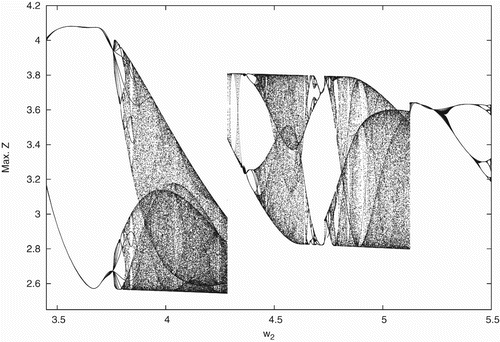
Figure 3. Bifurcation diagram with respect to w ₂∈(3.5, 5.5) for data set (17).

For the vector field X _η(x, 0, w, z), we consider the following data set:

Since the corresponding parameters in three-dimensional hyperspace Ω₄ and Ω₅ are identical for data sets (17) and (18), the bifurcation diagram with respect to w ₂∈(3.5, 5.5) is identical to Figure 3.

For the vector field X _η(x, y, w, z), the bifurcation diagram with respect to w ₂∈(3.5, 5.5) is identical to Figure 3 for the following set of data:

Since the corresponding parameters related to two middle predators competing for the bottom prey are identical, the vector field X _η(x, y, w, z) reduces to X _η(x, y+w, 0, z). Accordingly, the bifurcation diagrams in this case is obtained as shown in Figure 3. To further confirm the chaotic nature of system (2), the maximal Liapunov exponents for the bottom prey as a function of parameter w ₂ is drawn in Figure 4.

Figure 4. Maximal Liapunov exponent versus w ₂ for data set (19).

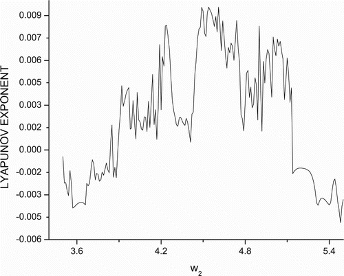
Observe that for w ₂∈(3.5, 5.5) in data set (19), the singularity E ₂=(0.206186, 1.02296, 0, 0) is an attracting focus (n ₁<0) in the x y-plane and has an unstable manifold along the z-axis (n ₃>0). The singularity E ₄=(0.57193, 0, 0, 1.6522) is attracting focus (n′′₁<0) in the x z-plane having an unstable manifold (n′′₂>0) in y-direction for w ₂∈(4.105, 5.5). Now, due to the first condition of Theorem 5.5, the three-dimensional subsystem X _η(x, y, 0, z) is uniformly persistent. The attractor for w ₂=5.0 for data set (19) in x y z-phase space is shown in Figure 5.

Figure 5. Attractor in the x y z-phase space for data set (19) at w ₂=5.0.

For the three-dimensional subsystem X _η(x, 0, w, z), the singularity E ₃=(0.206186, 0, 1.02296, 0) is also an attracting focus (n′₁<0) in the x w-plane and has an unstable manifold in the z-direction (n′₃>0). However, the singularity E ₄=(0.57193, 0, 0, 1.6522) is attracting focus (n′′₁<0) in thex z-plane having an unstable manifold (n′′₃>0) in the w-direction for w ₂∈(4.105, 5.5). Therefore, the three-dimensional subsystem X _η(x, 0, w, z) is uniformly persistent.

Now, for the data set (19), the singularities E ₂,  E ₃ and E ₄ of the system X _η(x, y, w, z) are attracting focus in respective coordinate planes having unstable manifolds in orthogonal directions. Due to conditions (13) of Theorem 6.1, the coexistence of all four species is obtained in this case. The attractors are drawn for various values of w ₂∈(4.104, 5.5). In particular, strange attractor is obtained for w ₂=5.0. The attractor is drawn in x y z-phase spaces in Figure 5. 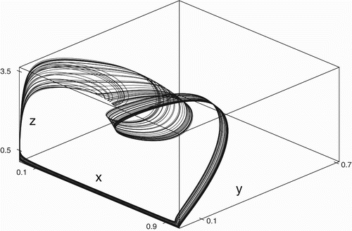Identical attractor is obtained in the x w z-phase space. From the figure, the denseness of the orbits clearly show the chaotic nature of the system and coexistence of all the four species in time.

It should be noted that the data in Equation (19) is symmetric (in parameters) about the middle predators (see data sets (17) and (18)). The data set (19) is now made asymmetric with slightly different death rates w ₅ and w ₁₃ as follows:

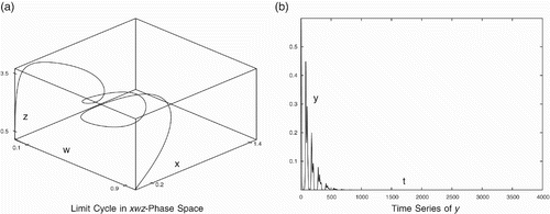
For the data set (20), the periodic orbit in the x w z-phase space and time series of predator y are shown in Figure 6. The coexistence of three species (x, w, z) and the extinction of predator y with time are evident. Similar observations were made for several other combinations of w ₅ and w ₁₃ also.

Figure 6. Periodic Behaviour for data set (20). (a) Limit cycle in x w z-phase space and (b) time series of y.

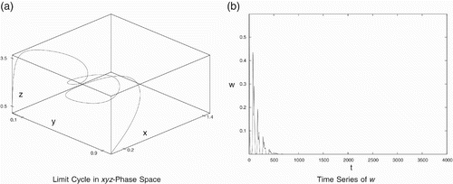
The middle predators (y and w) are in implicit competition due to the sharing of common prey~x. When other parameters are the same, the middle predator with higher conversion rate will be fitter than the other predator. Consider a set of data in which the conversion rate w ₄ of predator y is higher than to w ₁₄ of predator w:

Figure 7 shows the limit cycle in the x y z-phase space and the time series of predator w for the data set (21). The coexistence of three species (x, y, z) and the extinction of weaker predator w with respect to time are clearly evident. Similar observations were made for other combinations of conversion rates w ₄ and w ₁₄. In these conditions, the fittest of middle predators with higher conversion rate survives.

Figure 7. Periodic behaviour for data set (21). (a) Limit cycle in the x y z-phase space and (b) time series of w.

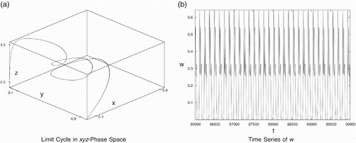
It is interesting to see that a small change in more than one parameters (asymmetries) may lead to coexistence of all the four species again. For example, we consider the following data set with different death rates and conversion rates:

The limit cycle in the x y z-phase space and the corresponding time series of predator w are shown in Figure 8. The dynamics of the system and the coexistence of all the four species in time are evident for this choice of parameters set (22).

Figure 8. Periodic behaviour for data set (22). (a) Limit cycle in the x y z-phase space and (b) time series of w.

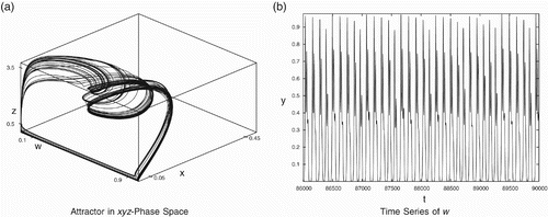
It is very interesting to observe that with more asymmetric data, all the four species may coexist. Also, it is possible to obtain many combinations of data around which the system may show the coexistence. In particular, consider the asymmetric data set:

The x w z attractor and corresponding y−t time series are shown in Figure 9 for data set (23). This clearly indicates the complexity of the system and the coexistence of all the four species in time. In the data sets (22) and (23), the complex interplay of parameters may be responsible for the coexistence of all the four species.

Figure 9. Complex dynamics for data set (23). (a) Attractor in the x y z-phase space and (b) time series of w.

8. Discussion

In this paper, a mathematical model is developed for a four-dimensional food-web system consisting of one prey population, two-middle predators feeding on the prey and one generalist predator feeding on all three other populations. The model does not consider any direct competition between the two middle predators, though they are in implicit competition through the shared predation on the bottom prey. The complex dynamic behaviour of the model incorporating nonlinear functional response is investigated. The solution initiating in the positive orthant is uniformly bounded and hence the system is dissipative. The system is decomposed in various subsystems under Kolmogorov conditions. The conditions for uniform persistence for three-dimensional subsystems has been established. In some cases, the extinction of one of the middle predator is observed in numerical simulations. However, the coexistence of all the four species is established when middle predators are symmetric in their interactions with other species. But the weaker of them will go to extinction in asymmetric cases. Some results regarding the existence of chaos have been established in special cases. For an open set of parameter space, the chaotic nature of the system is observed. Further, the coexistence of all the four species in the form of strange attractor is shown for suitable set of parameters. Numerical simulations suggest the coexistence of all the four species in asymmetric data. It may be possible due to inherent complex relationship between various parameters in the model.

Acknowledgements

We are thankful to anonymous reviewers for their valuable comments which has not only improved the quality of the paper but also significantly improved our understanding related to many concepts in this area. We also express our sincere thanks to Prof. Cushing for his valuable suggestions. The second author (A. Priyadarshi) wishes to thank ‘Ministry of Human Resources and Development (MHRD), India’ for a Senior Research Fellowship through Grant no. MHR02-23-200-304.

References

- Abrams , P. A. and Roth , J. D. 1994 . The effects of enrichment of three-species food chains with nonlinear functional responses . Ecology , 75 ( 4 ) : 1118 – 1130 .
- Andronov , A. A. 1973 . Qualitative Theory of Second-Order Dynamic Systems , New York : Halsted Press .
- Arrowsmith , D. K. 1990 . An Introduction to Dynamical Systems , Cambridge : Cambridge University Press .
- Butler , G. , Freedman , H. I. and Waltman , P. 1986 . Uniformly persistent systems . Proc. Amer. Math. Soc. , 96 : 425 – 430 .
- Angelis , D. L. 1975 . Stability and connectance in food web models . Ecology , 56 ( 1 ) : 238 – 243 .
- El-Owaidy , H. and Ammar , A. A. 1986 . Mathematical analysis of a food-web model . Math. Biosci. , 81 ( 2 ) : 213 – 227 .
- El-Owaidy , H. , Ragab , A. A. and Ismail , M. 2001 . Mathematical analysis of a food-web model . Appl. Math. Comput. , 121 : 155 – 167 .
- Freedman , H. I. 1980 . Deterministic Mathematical Models in Population Ecology , New York : Marcel Dekker .
- Freedman , H. I. and Hongshun , Q. 1988 . Interactions leading to persistence in predator–prey systems with group defence . Bull. Math. Biol. , 50 ( 5 ) : 517 – 530 .
- Freedman , H. I. and Ruan , S. 1995 . Uniform persistence in functional differential equations . J. Differential Equations , 115 : 173 – 192 .
- Freedman , H. I. and Waltman , P. 1984 . Persistence in models of three interacting predator–prey populations . J. Math. Biosci. , 68 : 213 – 231 .
- Gakkhar , S. and Naji , R. K. 2002 . Chaos in three species ratio dependent food chain . Chaos Solitons and Fractals , 14 ( 5 ) : 771 – 778 .
- Gakkhar , S. and Naji , R. K. 2003 . On a food web consisting of a specialist and a generalist predator . J. Biol. Syst. , 11 ( 4 ) : 365 – 376 .
- Gakkhar , S. and Naji , R. K. 2003 . Chaos in seasonally perturbed ratio-dependent prey–predator system . Chaos Solitons and Fractals , 15 ( 1 ) : 107 – 118 .
- Gakkhar , S. and Singh , B. 2005 . Complex dynamic behavior in a food web consisting of two preys and a predator . Chaos Solitons Fractals , 24 ( 3 ) : 789 – 801 .
- Guckenheimer , J. and Holmes , P. 1983 . Nonlinear Oscillations, Dynamical Systems and Bifurcations of Vector Fields , 8291 New York : Springer .
- Hastings , A. and Powell , T. 1991 . Chaos in a three-species food chain . Ecology , 72 ( 3 ) : 896 – 903 .
- Hogeweg , P. and Hesper , B. 1978 . Interactive instruction on population interactions . Comput. Biol. Med. , 8 ( 4 ) : 319 – 327 .
- Kumar , R. and Freedman , H. I. 1989 . A mathematical model of facultative mutualism with populations interaction in a food chain . J. Math. Biosci. , 97 : 235 – 261 .
- May , R. M. 1973 . Stability and Complexity in Model Ecosystems , Princeton , NJ : Princeton University Press .
- McCann , K. and Yodzis , P. 1994 . Biological conditions for chaos in a three-species food chain . Ecology , 75 ( 2 ) : 561 – 564 .
- McCann , K. and Yodzis , P. 1995 . Bifurcation structure of a three-species food-chain model . Theor. Popul. Biol. , 48 ( 2 ) : 93 – 125 .
- Rai , V. and Sreenivasan , R. 1993 . Period-doubling bifurcations leading to chaos in a model food chain . Ecol. Model. , 69 ( 1–2 ) : 63 – 77 .
- Scheffer , M. 1991 . Should we expect strange attractors behind plankton dynamics – and if so, should we bother? . J. Plankton Res. , 13 ( 6 ) : 1291
- Segel , L. 1984 . Modeling Dynamic Phenomena in Molecular and Cellular Biology , Cambridge : Cambridge University Press .
- Takeuchi , Y. 1996 . Global Dynamical Properties of Lotka–Voltera Systems , Singapore : World Scientific .
- Wilder , J. W. , Voorhis , N. , Colbert , J. J. and Sharov , A. 1994 . A three variable differential equation model for gypsy moth population dynamics . Ecol. Model. , 72 ( 3–4 ) : 229 – 250 .