Optimal strategy for controlling the spread of HIV/AIDS disease: a case study of South Africa

Abstract

HIV/AIDS disease continues to spread alarmingly despite the huge amounts of resources invested in fighting it. There is a need to integrate the series of control measures available to ensure a consistent reduction in the incidence of the disease pending the discovery of its cure. We present a deterministic model for controlling the spread of the disease using change in sexual habits and antiretroviral (ARV) therapy as control measures. We formulate a fixed time optimal control problem subject to the model dynamics with the goal of finding the optimal combination of the two control measures that will minimize the cost of the control efforts as well as the incidence of the disease. We estimate the model state initial conditions and parameter values from the demographic and HIV/AIDS data of South Africa. We use Pontryagin's maximum principle to derive the optimality system and solve the system numerically. Compared with the practice in most resource-limited settings where ARV treatment is given only to patients with full-blown AIDS, our simulation results suggest that starting the treatment as soon as the patients progress to the pre-AIDS stage of the disease coupled with appreciable change in the susceptible individuals’ sexual habits reduces both the incidence and prevalence of the disease faster. In fact, the results predict that the implementation of the proposed strategy would drive new cases of the disease towards eradication in 10 years.

Keywords:

• antiretroviral treatment
• basic reproduction number
• disease incidence
• disease prevalence
• optimal control
• Pontryagin's maximum principle
• optimality system

1. Introduction

Mathematical representation and analysis of infectious diseases have been central to infectious disease epidemiology. Now, mathematical models are being integrated with rigorous statistical methods to estimate the key model parameters and test hypotheses using available data 11 13. In the absence of reliable data, Mathematics is used to formulate hypotheses, inform data-collection strategies, and determine sample sizes. Optimal control theory is one area of Mathematics that is used extensively in the control of the spread of infectious diseases 9 16 22 31 32. It is a powerful mathematical tool that can be used to make decisions involving complex situations. Particularly, optimal control theory can be used in the control of the spread of most diseases for which there is either vaccination or treatment.

For example, Sethi and Staats 26 formulated some simple deterministic epidemic models for optimal control problems with the level of medicare programme effort and the level of inoculation programme effort as the control variables. They obtained the needed characterization of the optimal policies for the control of the epidemic over time using Pontryagin's maximum principle (PMP). Similarly, Gaff and Schaefer 7 applied optimal control theory to a series of epidemiological models in their attempt to find the most effective control strategy to minimize the number of individuals who become infected in the course of an epidemic using both treatment and vaccination as control measures.

Joshi et al. 16 used two examples to illustrate the concept of optimal control in two different disease models. In the first example, they showed how optimal control theory can be applied to find an optimal vaccination strategy that will minimize the size of the infectious population as well as the cost of vaccination. In the second example, they considered a model describing the interaction between the virus and the immune cell population in an individual under drug treatment, and they illustrated how optimal control theory can be used to determine a drug treatment strategy that minimizes the side effects of the drug together with the viral population at any point in time.

The work of Kirschner et al. 18 used the optimal control approach to determine the optimal strategy for the administration of reverse transcriptase inhibitors for HIV-positive individuals that minimizes the drug toxicity and their viral load while maximizing helper T-cell counts. In a related study, Fister and Donnelly 5 used optimal control theory to determine the condition for the elimination of tumour cells in individuals under treatment. Recently, Blayneh et al. 1 studied a deterministic model for the transmission dynamics of West Nile virus in the mosquito–bird–human zoonotic cycle using mosquito reduction strategies and human protection strategies as control measures. The numerical simulations of their resulting optimal control problem suggest that mosquito reduction strategies should be emphasized ahead of human protection measures in order to reduce the disease burden.

In this paper, we consider a deterministic for the spread of HIV/AIDS with a removed class that is made up of individuals who have sufficiently modified their sexual habits, thus making them literarily ‘immune’ to HIV infection by sexual contact. This differentiates the model from most of the existing models (see 14 17 23 25). We found the inclusion of this compartment justifiable because it is true that an appreciable number of people are now changing their sexual habits sufficiently due to the awareness of the widespread nature of the disease in society, the monumental deaths resulting from the disease, increasing knowledge of the agony and psychological trauma experienced by the infected individuals, and better enlightenment due to intense HIV/AIDS educational campaigns. Note that our proposed change in sexual habits does not imply that the removed individuals would no longer engage in sexual activities, rather this class of individuals would remain faithful to their sexual partners, reduce the number of the sexual partners to the barest minimum and avoid extra-marital affairs for the rest of their lives. We formulate our model as a fixed time optimal control problem with a view to finding the optimal combination of the control measures that will reduce the spread of the disease within a specified time period, since most governments usually set time frames for the accomplishment of the stated policy or objective.

This paper is organized as follows: In Section 2, we describe our proposed model. In Section 3, we establish the local and global stability of the model disease-free equilibrium. In Section 4, we estimate the model state initial conditions and parameter values. In Section 5, we formulate an optimal control problem subject to the model dynamics, characterize the optimal controls, and constitute its optimality system using PMP. In Section 6, we solve the resulting optimality system numerically and discuss our results.

2. Model equations

We consider a sexually active population N(t), divided into six compartments: S(t), H(t), P(t), A(t), T(t), and R(t). S(t) represents the number of susceptible individuals; H(t) represents the number of HIV-positive individuals in the asymptomatic stage of HIV infection; P(t) represents the number of HIV-positive individuals in the pre-AIDS stage but not receiving antiretroviral (ARV) treatment; A(t) represents the number of individuals with full-blown AIDS but not receiving ARV treatment; T(t) represents the number of individuals who are receiving ARV treatment; and R(t), the removed class, represents the number of individuals who have changed their sexual habits sufficiently such that they are, literarily, ‘immune’ to HIV infection by sexual contact. Note that the individuals in the R class are people who take up safe sexual habits and maintain the habits for the rest of their lives. The significance of the removed the R class is that it emphasizes the importance of prevention for a disease, such as HIV, that has no cure. Increasing the members in this class is one of the keys to controlling the spread of the disease.

A schematic diagram for the spread of the disease is shown in Figure 1.

Figure 1. A schematic diagram for the spread of HIV.

From Figure 1, the population dynamics is given by the following equations:

where N(t) denotes total population,

and N(t) satisfies the following equation:

The parameters for the model are defined in Table 1.

Table 1. Parameters used in the model.

Parameter	Description
Λ	Recruitment rate into the S class
d	Natural death rate
β1	Transmission rate for contact with the H class
β2	Transmission rate for contact with the P class ()
k 1	Progression rate from the H class into the P class
k 2	Progression rate from the P class into the A class ( k 1<k 2 )
u 1	Proportion of susceptible individuals who changed their sexual habits per unit time
u 2	Proportion of the P class receiving ARV treatment per unit time
u 3	Proportion of the A class receiving ARV treatment per unit time
δ1	Disease-induced death rate for AIDS individuals
δ2	Disease-induced death rate for the T class ()

Note that . However, under the dynamics described by Equation (1), the region Ω defined by

is positively invariant.

Lemma 1

The cone is positively invariant for the model (1) (i.e. the model does not predict negative values for the state variables at any future time).

Proof

Let . From Equation (1), we have

This is same as

and this implies that

Thus,

Hence,

Similarly, we can show that H(t)≥0, P(t)≥0, A(t)≥0, T(t)≥0, and R(t)≥0. This completes the proof.   ▪

The above lemma is important because it guarantees that the model variables are continuously biologically meaningful, since population size cannot be negative.

Lemma 2

Ω is a compact attracting set (i.e. the Ω limit set of any orbit starting in lies in Ω).

Proof

Using the non-negativity of the model state variables as established in the preceding lemma and

for initial conditions in and t≥0, we have This implies that

So, for all t≥0,

If is an Ω limit point of an orbit in , then there is a subsequence such that

Hence,

From Equation (4) (by evaluation at t=t _i and passing to the ), it follows that and hence that   ▪

Thus, for any initial starting point the trajectory lies in Ω. Therefore, the system is both mathematically and epidemiologically well posed.

3. Stability analysis

The system (1) has a disease-free equilibrium solution

and the model basic reproduction number, ℛ₀, is as given below:

Note that the basic reproduction number, ℛ₀, is the expected number of secondary infections arising from a single individual during his or her entire infectious period in a population of susceptible individuals 12. ℛ₀ is obtained using the next- generation matrix approach described in 4.

Theorem 1

The disease-free equilibrium is locally asymptotically stable if .

Proof

The Jacobian matrix of the system (1) is

where

  ▪

Evaluating the Jacobian matrix J at the disease-free equilibrium gives

The eigenvalues of J ₀ are

and we obtained λ₅ and λ₆ from the characteristic polynomial given below:

Taking a=1, , and

we have

Thus, we only need to show that b and c are positive in order for both λ₅ and λ₆ to be negative. However, implies that

Note that

and

Since c>0 and b>0, λ₅<0 and λ₆<0 if Therefore, the disease-free equilibrium is locally asymptotically stable if

Theorem 2

The disease-free equilibrium is globally asymptotically stable if .

Proof

We introduce the Lyapunov candidate function

Differentiating V(t) with respect to time yields

Substituting the model equations into Equation (9), we get

With and we have

Hence,

Choosing , we then find that

It is important to note that V̇=0 only when H=P=0. However, substituting H=P=0 into Equation (1) shows that , and as Applying LaSalle's invariance principle, every solution of the model (1), with initial conditions in Ω, converges to ℰ₀ 19 27. Hence, the disease-free equilibrium is globally asymptotically stable in Ω if .   ▪

4. Estimation of the model parameters and initial conditions

Each country has its own HIV/AIDS data. Here, we focus on South Africa, but the same analysis can be applied to other countries.

Initial conditions

The base year used in our simulations was 2006. The number of sexually active individuals (age 15–49 years) in South Africa was approximately 25.92 million in 2006. The number of HIV/AIDS-positive individuals in 2006 was 4.756 million. The number of individuals receiving ARV treatment was 0.511 million, and the number of AIDS-sick individuals not receiving ARV treatment was 0.2 million 3. Thus, we took A(0)=0.2 million, T(0)=0.511 million, and million. We assumed that H(0)=2P(0), so that H(0)=2.697 million and P(0)=1.348 million. Since N(0)=25.92 million, we also had million.

Parameter values

Constant recruitment rate (Λ). This was estimated as the net births that occurred 15–20 years ago plus the present net migration. The net births were calculated using the average of births in South Africa between 1990 and 2000 since this gives a good rough estimate of the group of individuals who will become sexually active after the year 2005. The birth value obtained was adjusted with the infant mortality rate over the same period (Table 2). According to United Nations 30, the crude births in South Africa for 1990–1995 and 1995–2000 were 27.5 and 25.2 per thousand population, respectively, while the infant mortalities were 50.4 and 56.8 per thousand live births, respectively. Thus, we got an average of 26.3 per thousand population for the crude births and 53.6 for the infant mortality per thousand live births. We used the number of people in South Africa in 1990, which was 36.747 million, to estimate the births during 1990–2000. Also, the net annual migration into South Africa between 2000 and 2010 was 140, 000. Therefore, we computed the constant recruitment rate (Λ) as follows:

Table 2. Parameter values obtained using data from South Africa.

Parameter	Units	Value	Reference
Λ	Population/year	1.04	3 and estimate
d	yr^−1	0.0196	28
β1	yr^−1	0.11	Estimate
β2	yr^−1		10 and estimate
k 1	yr^−1	0.198	10 and estimate
k 2	yr^−1	0.4621	10 and estimate
u 1	yr^−1		Variable
u 2	yr^−1		Variable
u 3	yr^−1		Variable
δ1	yr^−1	0.0909	Estimate
δ2	yr^−1	0.0667	Estimate

Natural death rate (d). This was estimated using the life expectancy for a South African at birth who was 51 years old in 2006 28. Based on the assumption that if the population were to be normally distributed, 1 in every 51 persons will die every year. Thus, we estimated .

Progression rates (k ₁, k ₂). Following 10, we assumed that it takes 7 years for a newly infected person to progress to the pre-AIDS stage and 3 more years to develop full-blown AIDS. Therefore, we obtained and

Disease-induced death rates . Based on their analyses of findings from several studies conducted mostly in Africa to examine the survival period of HIV patients from seroconversion to death before ARV treatment becomes available, Ghys et al. 8 recommended that an average survival period of 11 years be used in modelling national epidemics. Thus, we computed . There is overwhelming evidence that ARV therapy substantially extends the life of HIV/AIDS patients 8 9. Thus, we assumed that ARV treatment will extend the life of patients for an additional 4 years. Thus, the survival period for HIV-infected individuals under ARV treatment was estimated as 15 years. We computed .

Transmission rates . It is known that the infection rate (β₁) of individuals from the H class is smaller than the infection rate (β₂) of individuals from the P class 10. We assumed that According to Dorrington et al. 3, the prevalence of HIV/AIDS among adults in South Africa for the year 2006 was 18.3%. In order to determine β₂, we used the Berkeley Madonna software for parameter fitting. We solved the system (1) with the initial conditions and the parameters (except β₂) as determined above and determined β₂, which yields π=18.3%, namely

5. Optimal control problem formulation

Our objective functional is defined by

subject to the system of Equations (1) with appropriate state initial conditions, and t _f is the final time, while the control set 𝕌 is defined as

and the weight constants w ₁, w ₂, w ₃, w ₄, w ₅, w ₆, and w ₇ are the relative weights and help to balance each term in the integrand so that any of the terms do not dominate. Here, it is important to note that w ₁, w ₂, and w ₃ are the relative measures of the cost or effort required to implement each of the associated controls, while w ₄, w ₅, w ₆, and w ₇ are the relative measures of the importance of reducing the associated classes on the spread of the disease and its burden.

The lower bounds for u ₁, u ₂, and u ₃ correspond to no change in sexual habits, no ARV treatment for the P class, and no ARV treatment for the A class, respectively, while the upper bound for each of the controls , and u _3max) will depend on the budget allocated for the execution of each of the control measures. For instance, we shall hypothetically set u _1max=0.2, u _2max=0.5, and u _3max=0.5 in our subsequent simulations. We wish to determine the optimal combination of controls u ₁, u ₂, and u ₃ that will be adequate to minimize the cost of the education/enlightenment campaign together with the cost of ARV treatment as well as to reduce the incidence of the disease over a fixed time period. Note that S was included in the integrand to emphasize the need for reducing the susceptible individuals in addition to the infective individuals, particularly for a disease without cure. Moreover, S contributes to the incidence of the disease together with H and P. We also included A in the integrand to indirectly reduce AIDS-induced deaths.

5.1 Existence of an optimal control pair

Here, we examine the sufficient conditions for the existence of a solution to the optimal control problem.

Theorem

There exists an optimal control set with a corresponding solution to the model system (1) that minimizes J(u ₁, u ₂, u ₃) over 𝕌.

Proof

The existence of the optimal control is guaranteed by the compactness of the control and the state space and the convexity in the problem based on Theorem 4.1 of Chapter III and its corresponding corollary in 6. The following non-trivial requirements from Fleming and Rishel's theorem are stated and verified:

	(1) The set of all solutions to Equation (1) and its associated initial conditions together with the corresponding control functions in 𝕌 is non-empty.
	(2) The state system can be written as a linear function of the control variables with coefficients dependent on time and state variables.
	(3) The integrand L in Equation (14) is convex on 𝕌 and additionally satisfies where c 1, c 2>0 and α>1.

We refer to Theorem 3.1 proposed by Picard–Lindelof in 2. Based on this theorem, if the solutions to the state equations are a priori bounded and if the state equations are continuous and Lipschitz in the state variables, then there exists a unique solution corresponding to every admissible control set in 𝕌. Using the fact that for all , all the model states are bounded below and above, the solutions to the state equations are bounded. In addition, the boundedness of the partial derivatives with respect to the state variables in the system can be directly shown, and this shows that the system is Lipschitz with respect to the state variables. Thus, condition 1 holds. As we can observe from the state equations (1), the state equations are linearly dependent on the controls u ₁, u ₂, and u ₃. Thus, condition 2 also holds. To establish condition 3, we observe that the integrand L in our objective functional is convex since it is quadratic in the controls. Then, we only need to prove the bound on L. This is shown as follows:

The above then establishes a bound on L. Thus, we have a unique solution of the optimality system for small time intervals due to the opposite time orientations of the state equations and the adjoint equations. Moreover, the uniqueness of the solution of the optimality system guarantees the uniqueness of the optimal control if it exists.   ▪

5.2 Characterization of the optimal controls

We characterize the optimal controls u ₁*, u ₂*, and u ₃*, which gives the optimal levels for the various control measures and the corresponding states The necessary conditions for the optimal controls are obtained using PMP 24.

Theorem 4 (Necessary conditions)

Let be an optimal control with the corresponding states S*, H*, P*, A*, T*, and R*. Then, there exist the adjoint variables λ _i for i=1, …, 6, which satisfy

and the transversality conditions

with the optimal controls defined as follows:

Proof

Using PMP, we obtain Equation (17) from

where the Hamiltonian ℍ is given by

The transversality conditions have the form (18), since all the states are free at the terminal time. The Hamiltonian is maximized with respect to the controls at the optimal control , thus we differentiate ℍ with respect to u ₁, u ₂, and u ₃ on 𝕌, respectively, to obtain

Hence, solving for u ₁*, u ₂*, and u ₃* on the interior sets gives

We can now impose the bounds , , and on the controls to get

  ▪

It is important to note that the characterization of the above controls can be written in a simpler piecewise form given below:

We can now solve the optimality system that consists of the state system (1) with its associated initial conditions and the adjoint system (17) with its transversality conditions coupled with the control characterizations (26)–(28).

6. Numerical results and discussion

We numerically solved the resulting optimality system – a two-point boundary value problem – using a fourth-order iterative Runge–Kutta scheme. This method solves the state equations with an initial guess for u ₁, u ₂, and u ₃ forward in time, after which it solves the adjoint equations backward in time, and then the controls are updated using Equations (26)–(28). This computational procedure is done iteratively until a convergence is attained. Details on the forward- and backward-sweep procedure are given in 20. We simulated our model with the data described below.

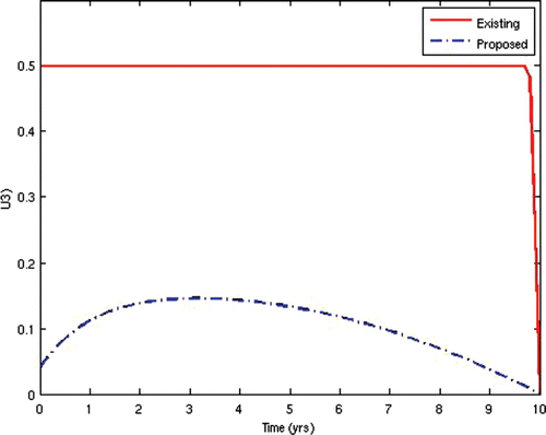
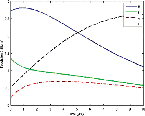
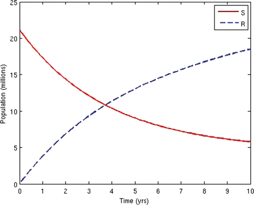
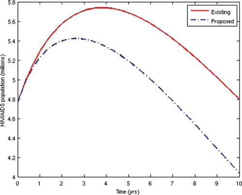
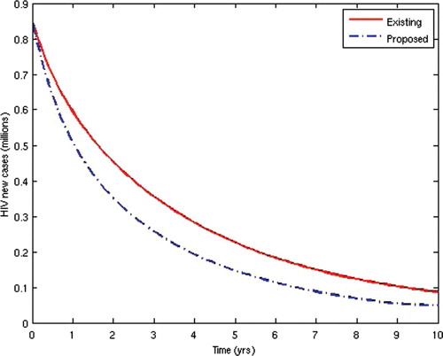
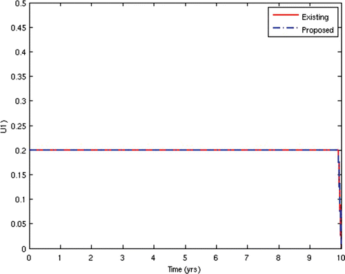
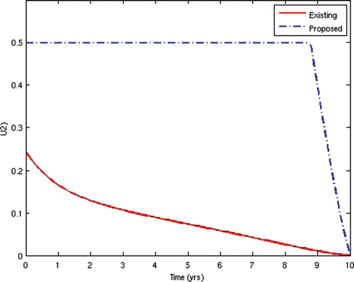
We investigated the dynamics of the disease compartments for varying combinations of the weight constants w ₁, w ₂, w ₃, w ₄, w ₅, w ₆, and w ₇, with the assumption that the resources available can only accommodate the following maximum levels of the controls: u _1max=0.2, u _2max=0.5, and In the first scenario, we set w ₁=1.0, w ₂=1000, w ₃=10, w ₄=1, w ₅=10, w ₆=10, and w ₇=50. This scenario corresponds to the present situation in most developing countries where ARV treatment is only given to the AIDS-sick individuals, while the pre-AIDS individuals have to wait until they develop full-blown AIDS before they can be given the treatment. This is often the case in situations where branded ARV drugs (usually very expensive) are mostly used for the treatment and the medical personnel and facilities required for the administration of the treatment are grossly inadequate, thus prompting the government to make the treatment available to only the patients who need it the most. The population profiles of the different disease compartments and the disease-free compartments for this case are shown in Figures 2 and 3, respectively.

Figure 2. Population of the different disease classes with u ₂ ≈ 0 and u ₃=0.5.

Figure 3. Population of the disease-free classes (S, R) with u ₂ ≈ 0 and u ₃=0.5.

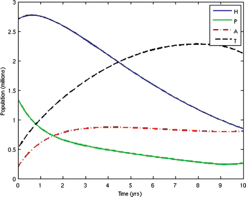
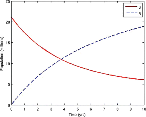
In the second scenario, we alternated the values of the weights w ₂ and W ₃ and fixed the other weights. Thus, we set w ₂=10 and w ₃=1000. This scenario corresponds to the situation where HIV-infected individuals are given ARV treatment as soon as they progress to the pre-AIDS stage without waiting for the onset of AIDS. This is presently not the case in many resource-limited countries. This would be the situation in societies where generic versions (considerably cheaper) of ARV drugs are used as substitutes for the branded ones, while there are adequate medical personnel and facilities to enable a wide coverage of ARV treatment. In this instance, the cost of initiating ARV treatment at the pre-AIDS stage is significantly reduced. This strategy obviously prolongs the lifespan of HIV/AIDS patients and delays the onset of AIDS. However, the AIDS cases in this scenario are usually very serious and a lot more expensive to manage due to the patients’ development of resistance to most of the first-line and second-line ARV drugs, thus leaving the doctors no options other than patients’ hospitalization and use of very expensive ARV drugs.

The population profiles of the different disease compartments and the disease-free compartments for this case are shown in Figures 4 and 5, respectively.

Figure 4. Population of the different disease classes with u ₂=0.5 and u ₃ ≈ 0.

Figure 5. Population of the disease-free classes (S, R) with u ₂=0.5 and u ₃ ≈ 0.

Now, we consider the prevalence and incidence of the disease for the two scenarios. Figures 6 and 7 show the prevalence and incidence for each of the two cases, respectively.

Figure 6. The disease prevalence for each of the two scenarios.

Figure 7. The disease incidence for each of the two scenarios.

From the above results, we can observe that the administration of ARV treatment to HIV-infected individuals before they become AIDS sick reduces both the prevalence and the incidence of the disease faster than in the case where we wait until they become AIDS sick before we give them the treatment (Figures 8–10). The expenses that will be incurred by starting ARV treatment earlier will be compensated for by the remarkable reduction in the prevalence and incidence in the later years. Thus, it will be cheaper in the long run to commence ARV treatment at the pre-AIDS stage for the infected population.

Figure 8. Control u ₁ for the two scenarios.

Figure 9. Control u ₂ for the two scenarios.

Figure 10. Control u ₃ for the two scenarios.

Remark

The two scenarios simulated were specifically chosen to demonstrate that the case where ARV treatment is given to patients after they have developed full-blown AIDS, as practised in most resource-limited settings. This may not be helpful in reducing the spread of the disease. Rather, an alternative approach of starting the treatment as soon as the patients progress to the pre-AIDS stage of the disease would be better.

7. Conclusion

We presented a deterministic model for controlling the sexual spread of HIV/AIDS disease. We established that the model disease-free equilibrium is locally and globally asymptotically stable, if the basic reproduction number is less than unity. We formulated an optimal control problem subject to the model dynamics with change in the susceptible individuals’ sexual habits due to education/enlightenment campaigns and the administration of ARV treatment to the pre-AIDS and the AIDS-sick individuals as controls. Our aim is to find an optimal strategy that will minimize the cost of implementing the combined control programmes as well as the incidence of the disease.

We proved the existence and uniqueness of the optimal control and we characterized the controls using PMP. The resulting optimality system was solved numerically; the results show that the optimal way to mitigate the spread of the disease is for susceptible individuals to consistently practise safe sex as much as possible, while ARV treatment should be initiated for patients as soon as they progress to the pre-AIDS stage of the disease. This strategy may be expensive at the outset, but it is optimally cost effective in the long run and it portends more benefits for the HIV/AIDS individuals and the society at large.

Acknowledgements

This work was supported by the National Science Foundation African Biomathematics initiative Grant Award 6RT00014792. The authors acknowledge the support of the German Academic Exchange Service (DAAD) scholarship award for this work. Also, the first author thanks the Mathematical Biosciences Institute (MBI), Ohio State University, for providing research facilities towards the completion of this work. The authors thank Avner Friedman, S. Lenhart and R. Leander for their useful discussions on the work and also appreciate the anonymous reviewers for their constructive suggestions.

References

- Blayneh , K. W. , Gumel , A. B. , Lenhart , S. and Clayton , T. 2010 . Backward bifurcation and optimal control in transmission dynamics of the West Nile virus . Bull. Math. Biol. , 72 : 1006 – 1028 .
- Coddington , E. A. and Levinson , N. 1955 . Theory of Ordinary Differential Equations , New York : McGraw Hill .
- Dorrington , R. , Johnson , L. , Bradshaw , D. and Daniel , T. The demographic impact of HIV/AIDS in South Africa: National and provincial indicators for 2006 , Cape Town : Centre for the Actuarial Research, South African Medical Research Council and Actuarial Society of South Africa .
- Driessche , P. V. and Watmough , J. 2002 . Reproduction numbers and sub-threshold endemic equilibria for compartmental models of disease transmission . Math. Biosci. , 180 : 29 – 48 .
- Fister , K. R. and Donnelly , J. H. 2005 . Immunotherapy: An optimal control theory approach . Math. Biosci. Eng. , 2 : 499 – 510 .
- Fleming , W. H. and Rishel , R. W. 1955 . Deterministic and Stochastic Optimal Control , New York : Springer-Verlag .
- Gaff , H. and Schaefer , E. 2009 . Optimal control applied to vaccination and treatment strategies for various epidemiological models . Math. Biosci. Eng. , 6 : 469 – 492 .
- Ghys , P. D. , Basia , Z. and Prins , M. 2007 . Survival and mortality of people infected with HIV in low and middle income countries: Results from the extended ALPHA network . AIDS , 21 ( Suppl. 6 ) : S1 – S4 .
- Gilks , C. F. , Crowley , S. , Ekpini , R. , Gove , S. , Perriens , J. , Souteyrand , Y. , Sutherland , D. , Vitoria , M. , Guerma , T. and De Cock , K. 2006 . The WHO public-health approach to antiretroviral treatment against HIV in resource-limited settings . Lancet , 368 : 505 – 510 .
- Granich , R. M. , Gilks , C. F. , Dye , C. , De Cock , K. M. and Williams , B. G. “ Universal voluntary HIV testing with immediate antiretroviral therapy as a strategy for elimination of HIV transmission: A mathematical model ” . The Lancet . published online 26 November (2008), doi:10.1016/S0140-6736(08)61697-9
- Grassly , N. C. and Fraser , C. 2008 . Mathematical models of infectious disease transmission . Nat. Rev. Microbiol. , 6 : 477 – 487 .
- Heffernan , J. M. , Smith , R. J. and Wahl , L. M. 2005 . Perspectives on the basic reproduction ratio . J. R. Soc. Interface , 2 : 281 – 293 .
- Hethcote , H. W. 2000 . The Mathematics of Infectious Diseases . SIAM Rev. , 42 : 599 – 653 .
- Hsieh , Y. and Sheu , S. 2001 . The effect of density-dependent treatment and behaviour change on the dynamics of HIV transmission . J. Math. Biol. , 43 : 69 – 80 .
- Joshi , H. , Lenhart , S. , Albright , K. and Gipson , K. 2008 . Modeling the effect of information campaign on the HIV epidemic in Uganda . Math. Biosci. Eng. , 5 : 757 – 770 .
- Joshi , H. , Lenhart , S. , Li , M. Y. and Wang , L. 2006 . Optimal control methods applied to disease models . Contemp. Math. , 410 : 187 – 207 .
- Kgosimore , M. and Lungu , E. M. 2006 . The effects of vertical transmission on the spread of HIV/AIDS in the presence of treatment . Math. Biosci. Eng. , 3 : 297 – 312 .
- Kirschner , D. , Lenhart , S. and Serbin , S. 1997 . Optimal control of the chemotherapy of HIV . J. Math. Biol. , 35 : 775 – 792 .
- Lasalle , J. P. 1976 . The stability of dynamical systems , Philadelphia : SIAM .
- Lenhart , S. and Wortman , J. T. 2007 . Optimal control applied to biological models , Boca Raton , FL : Taylor & Francis .
- Mukandavire , Z. and Garira , W. 2007 . Sex-structured HIV/AIDS model to analyse the effects of condom use with application to Zimbabwe . J. Math. Biol. , 54 : 669 – 699 .
- Nanda , S. , Moore , H. and Lenhart , S. 2007 . Optimal control of treatment in a mathematical model of chronic myelogenous leukemia . Math. Biosci , 210 : 143 – 156 .
- Naresh , R. , Tripathi , A. and Omar , S. 2006 . Modelling the spread of AIDS epidemic with vertical transmission . Appl. Math. Comput. , 178 : 262 – 272 .
- Pontryagin , L. S. , Boltyanskii , V. G. , Gamkrelidze , R. V. and Mishchenko , E. F. 1986 . The Mathematical Theory of Optimal Processes , New York : Gordon and Breach Science Publishers .
- Rao , A. S. , Thomas , K. , Sudhakar , K. and Maini , P. K. 2009 . HIV/AIDS epidemic in India and predicting the impact of the national response: Mathematical modeling and analysis . Math. Biosci. Eng. , 6 : 779 – 813 .
- Sethi , S. P. and Staats , P. W. 1978 . Optimal control of some simple deterministic epidemic models . J. Oper. Res. Soc. , 29 : 129 – 136 .
- Tewa , J. J. , Dimi , J. L. and Bowong , S. 2009 . Lyapunov function for a dengue disease transmission model . Chaos Solitons Fractals , 39 : 936 – 941 .
- UNAIDS/WHO . Epidemiological fact sheet on HIV and AIDS: Core data on epidemiology and response. South Africa 2008 Update Available at www.unaids.org or www.who.int/hiv
- UNAIDS/WHO . AIDS epidemic update: November 2009 Available at www.unaids.org or www.who.int/hiv
- United Nations . 2009 . World Population Prospects: The 2008 Revision Population Database Available at http://esa.un.org/unpp
- Vladimir , M. V. 2008 . Optimal Control of heterogeneous systems: Basic theory . J. Math. Anal. Appl. , 346 : 227 – 242 .
- Yan , X. , Zou , Y. and Li , J. 2007 . Optimal quarantine and isolation strategies in epidemics control . World J. Model. Simul. , 3 : 202 – 211 .
- Zaman , G. , Kang , Y. H. and Jung , I. H. 2008 . Stability analysis and optimal vaccination of an SIR epidemic model . BioSystems , 93 : 240 – 249 .