Estimating von Bertalanffy parameters with individual and environmental variations in growth

Abstract

Variation among individuals is an ubiquitous feature of natural populations. However, the relative roles of intrinsic individual differences and stochastic processes in generating variation remain poorly understood. For somatic growth, identifying the contribution of individual and stochastic processes to observed variation in size has important implications both for basic and applied biology. Here we propose and develop methods for estimating individual variation in growth using size-at-age data. We modify the von Bertalanffy growth model to explicitly incorporate individual, environmental, and stochastic variation and provide analytic expressions for the mean and variance of length-at-age in populations. We use a Bayesian statistical model to estimate individual variation from length-at-age data and apply the model to simulated data to test its efficacy. Although a first step towards understanding individual variation, we demonstrate that estimating individual variation from observational samples is possible and provide a platform for future analytical and statistical developments.

Introduction

Better understanding of the biology of growth will always be a challenge. Individual variability is a fundamental component of biological systems that has important implications for both evolutionary and ecological dynamics. On ecological scales, individual variation can alter predictions from population models 5 25 69 and affect the estimation of parameters that are vital for management and conservation (e.g. estimates of somatic growth; 51 60). In evolutionary terms, the rate of phenotypic and genotypic change depends strongly on the individual variation present in populations as well as the heritability and plasticity of traits, and the strength of selection 41. The presence of individual variation in natural populations is likely an indicator of life-history tradeoffs and/or bet-hedging strategies. For example, the persistence of individual variation in populations may be an indicator of negative-frequency dependence 26 40, an interaction between traits and a variable environment 24, or equivalent fitness between alternative life-history strategies 65, among other mechanisms. Furthermore, it is increasingly evident that human-driven selection can substantially and rapidly affect the genotypes and phenotypes present in populations 9 13. Together, these facts motivate the investigation of individual variation in natural populations.

Evidence from across many taxonomic groups demonstrates individual differences are common in natural populations 8. Plant biologists have long noted the persistent variation individuals in growth and reproductive output 29 61 62 72. Studies of mammals have illustrated persistent individual differences in growth, maternal quality, and behaviour 8 66 67. Similar observations have been made among fish 45 59. Among invertebrates, there is evidence that individual specialization on different prey items that may have population consequences 47 73. The possible consequences of individual variation for management have been acknowledged (e.g. for fisheries management: 57 58 60; for conservation biology: 10 51 52), but few efforts have been made to explicitly estimate individual variation and incorporating it into management (but see 28 48 53).

A common and important occurrence of individual variation is in the context of somatic growth 15 50 51. Individual variation in growth can arise from a variety of processes. Two examples include individuals within a population varying in their intrinsic metabolic rates 2–4,45 49 and individuals varying in behavioural traits (e.g. aggressiveness or territoriality; 43 59, Brikead 2008). Both metabolic and behavioural traits can be heritable, but are certainly not perfectly inherited. Realized growth is a combination of an individual's genetic background, the environmental conditions an individual experiences, and stochastic forces 41. Methods that seek to document and understand individual variation in growth must account for these three distinct forces.

The complexity of variation in growth has promoted a diversity of approaches taken to look at individual variation in growth. In the theoretical context, models for growth range from approaches based on partial differential equations 15 27 to individual-based simulations (51, reviewed by DeAngelis and Mooij 14), to detailed physiological models of growth 22 37 39.

A major challenge in understanding individual growth is determining how to connect these models to the available data. Estimating the amount of individual variation is a complex biological and statistical problem 15 38 41 50. In particular, distinguishing variation arising from true individual differences from variation arising from stochastic processes can be very difficult as multiple processes may produce very similar patterns in natural populations 17 48. Thus, estimating individual variation usually requires individual level data. However, data on individuals derived from mark-recapture studies are difficult to collect and for many species may be logistically impossible 7. A common data source in many ecological situations are longitudal surveys where a sample of representative individuals are collected at regular intervals. While such time-series will never provide the details available from individuals 8, the abundance of observational data motivates the development of methods to extract additional biological inference from such sources.

Here we focus on the development of methods for estimating individual variation in growth from observational data. We build a flexible framework for assessing individual variation in growth that builds from basic physiological assumptions. We balance the desire for biologically complex models with large numbers of parameters that may be only weakly statistically identifiable (e.g. bioenergetic models of Kitchell et al. 37, Essington et al. 18, and Harvey 30 or dynamic energy budget models of Kooijman 39 and Nisbet et al. 46) and the desire for simple statistically rigorous models that cannot incorporate individual varation 20. We highlight the assumptions made by investigators when they incorporate individual variation into standard growth models and provide biological interpretations for some of the most common assumptions about individual variation.

We present our paper in four sections: (1) motivation and description of a basic individual growth model; (2) incorporating individual variation and environmental variation into the growth model; (3) developing a Bayesian statistical model for estimating individual level traits from observational data; (4) testing the efficacy of our approach, using simulated data.

Happy Birthday Simon!

We are delighted to contribute to this issue in honour of the birthday of Simon Levin, a longtime friend (since 1977) of one of us (Mangel). In the late 1980s, both Mangel and Levin worked independently on the temporal and spatial dynamics of southern ocean krill Euphausia superba (the superb krill), as the Commission for the Conservation of Antarctic Marine Living Resources (CCAMLR) wrestled – as it continues to do – with the problem of managing the krill fishery so that dependent predators were not adversely affected by the fishery. Although Simon left krill-related work shortly thereafter, Mangel continues on it to this day.

Krill can be effectively aged by the size of their eyes, and when captured in the field (or even grown in tanks), krill of the same age show distributions in size 6 34 and understanding the sources of those distributions has implication for management of the krill fishery 1, predictions of the effects of climate change on krill biomass available for predators 74, and more fundamental questions such as how maturity is regulated for organisms living in a seasonal environment 35.

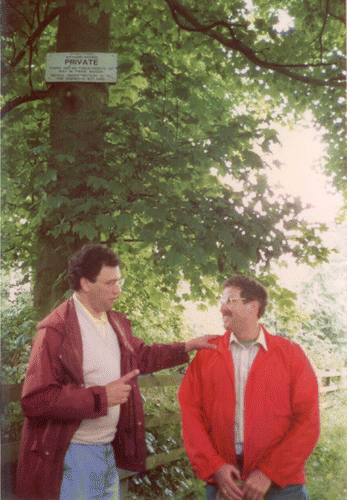
Levin and Mangel also spent part of their sabbatical year 1987–1988 at the University of Oxford, much time was spent discussing biological dynamics (Figure 1).

Figure 1. Simon Levin instructing Marc Mangel on aspects of biological dynamics during an outing in Whytam Woods, University of Oxford, Spring 1988.

Methods

Growth model

Our starting point is the most commonly used model of growth, the von Bertalanffy growth function (VBGF; 2 4). The rate of growth of an individual of length x

where q is a coefficient of anabolism and k is a coefficient of catabolism (commonly known as the von Bertalanaffy growth coefficient). We refer readers to von Bertalanffy 2 4, Essington et al. 18, or Mangel 44 for a more complete discussion of the derivation of the VBGF. The more commonly used form of the VBGF is

Here, , the asymptotic length, replaces q as the second parameter.

The important difference between these equations is that the two parameters in Equation (2), k and L _∞, are not independent, which is often forgotten in the analysis of growth and problematic in the context of understanding individual variation. For example, assuming one parameter (e.g. L _∞) is fixed for all individuals and the other (k) varies among individuals 53 54 makes specific assumptions about the process of growth that are not generally acknowledged (e.g. that q is directly proportional to k). Assuming the converse relationship (L _∞ random and k fixed for individuals), makes a very different set of biological assumptions. While these assumptions may have relatively small consequences for the estimation of some management relevant quantities such as mean length-at-age 19, in the context of understanding individual variation in growth, these assumptions are very important (see Methods: Incorporating individual and environmental variation).

Thus, in Equation (2) L _∞ and k should be strongly correlated when estimated from data (as noted by many authors, e.g. Pilling et al. 53, Helser and Lai 32, Siegfried and Sansó 63, Helser et al. 33, and Eveson et al. 19). The persistence of the negative correlation is a result at least in part of the parameterization of the VBGF, not necessarily any biologically interesting or important mechanism (see also 19 53 55).

To begin, we illustrate how Equation (1) provides an intuitive way to incorporate individual variation into growth. We integrate Equation (1) with the initial condition x(0)=x ₀ and add the subscript i to make explicit that growth is an individual process to obtain

We assume that among individuals in the population, the distributions of q and k are strictly positive so the expected length in the population at time t, E[x(t)], is

where f(k) and g(q) indicate the probability density function for q and k among individuals, respectively. If f(k) is a Gamma distribution with parameters 1 g(q) is any positive distribution with mean , and q and k are independent, the expected length in the population is

where is the mean von Bertalanffy coefficient among individuals in the population. In the supplementary information, we give the general analytic solution for the variance of length at t.

If x ₀ is very small (), the first term in this equation is effectively 0. Large values of α indicate low individual variability while small values indicate high among individual variation (for reasonable results, α> 1) so as individual variability declines, , this equation collapses to the standard VBGF with no individual variation. While it is not immediately obvious from Equation (5), the expected length in the population at a given t in a population with no individual variation is always greater than the asymptotic length when variation in k is present 60, due to Jensen's inequality 16. Thus, failing to account for individual variation will lead to biased estimates of growth parameters and biased estimates of length-at-age, as previously noted by Sainsbury 60, Francis 21, Wang 70, and Eveson et al. 19. However, the amount by which the expected length declines in the presence of individual variation depends strongly on the amount of variation present in k in the population (i.e. the magnitude of α). Furthermore, there are biological reasons for k and q to be inter-related and not independent, so we now turn to a model that combines individual and environmental variation and allows for dependence between q and k.

Incorporating individual and environmental variation

Because q _i is the parameter of anabolism, it should be closely linked to bottom-up factors in the environment such as food availability. The parameter k _i determines how metabolic rates scale with an individual's size and, therefore, relates to an individual's phenotypic capacity for growth and, for ectotherms, should be related to temperature. We follow Snover et al. 64 65 and assume that k _i combines physiological and behavioural traits that determine individual activity and, therefore, affect the ability of an individual to obtain resources from the environment. Under this assumption, we model q _i as a function of k _i 64 65. To do so, we let γ to be a parameter describing the condition of the environment common to all individuals and ψ be a parameter that determines the degree to which q _i depends on environmental versus individual factors, and set

We treat ψ as a population-level parameter so that all individuals are assumed to have a shared value. We constrain ψ to the interval [0,1] (see 65). The effect of ψ on growth for individuals with different k _i can be considerable (Figure 2). If ψ=0, k _i and q _i are independent and individual activity has no affect on an individual's success at obtaining resources from the environment; all individuals experience an identical environment, γ. Therefore, when ψ=0 individuals with large k _i will have lower realized growth increments (Figure 2(a)). At the other extreme, ψ=1, aggressive or highly active individuals (large k _i ) always have greatly increased access to resources, and therefore experience faster length-specific growth (Figure 2(c)). For intermediate values of ψ, the relative growth rate for each individuals with different k _i will change with an individual's length. Individuals with large k _i will grow faster at small lengths and individuals with small k _i will grow faster at large size (Figure 2(b)), and the length at which individuals experience equivalent growth depends on ψ.

Figure 2. Expected growth increments (Δ x) for three individuals with fixed differences in k across a range of values for ψ. All individuals were assumed to have a starting length of 1 and live in a constant environment. The x-intercept of each line corresponds to an individual expected asymptotic length, L _∞. Each growth trajectory was calculated from Equation (7) using a constant value of γ scaled such that k=0.10 always has L _∞=100. (a) ψ=0, (b) ψ = 0.5, and (c) ψ=1.0.

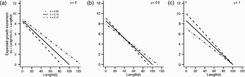
Equation (6) connects directly to previous attempts to account for individual variation in statistical analyses of growth. Assuming k is variable among individuals and L _∞ is fixed for all individuals 19 54 is a special case of Equation (6) when ψ=1 (Figure 2(c)). Treating only L _∞ as a random variable with k fixed among individuals 19 42 70 71 assumes that each individual experiences a distinct environment (q _i ) that persists throughout an individual's life (Figure A1). This assumption may be reasonable for some sessile organisms, where micro-habitat differences may wholly determine an individual's growth, but is less likely for most mobile animals, including mammals, birds, or fish, that are competing for resources on a heterogeneous landscape. Nearly all attempts to model both k and L _∞ as random variables treat these parameters as independent (e.g. 19 42, but see 68); they are are inconsistent with the physiological foundations of the VBGF and mathematically wrong.

Behavioural characteristics (e.g. the amount of dominance) vary among species and potentially among populations within a species, so we expect ψ to vary as well. In most instances, we lack direct information about the importance of dominance to species growth and thus need methods to help inform the contribution of behavioural traits to growth.

Variable environments are the rule in natural systems and can have significant effects on growth 22 31. Variable environments can by incorporated by allowing γ to differ among time intervals. If γ _t indicates the environmental conditions for an interval ending at time t, then we set . Thus, we interpret q _{i, t} as the realized growth conditions for an individual during the interval ending at time t, given the environmental conditions and the individual's traits. The parameter γ _t is shared by all individuals but can vary among time periods. While we will not implement it here, γ _t could be written as a function of environmental covariates (e.g. temperature) instead of as a series of discrete states (see 36 for a similar approach using the standard parameterization of the VBGF). We choose the time interval sufficiently small that γ _t can be treated as constant between t−1 and t we can write a discrete time map for length

Equation (7) describes growth as a deterministic process. However, stochastic processes also contribute to growth. For example, finding a particularly rich food source is most generally a function of the environmental conditions, individual traits, and luck; the contribution of stochastic variation most generally scales with the quality of the environment and the individual. When an individual is small, the second term in Equation (7) is much larger than the first term and the environment plays a predominant role in determining the size in the following time period. If an individual is large, x _i (t−1) is closer to the asymptotic length and the second term contributes relatively less to size in the following year. Thus, the relative contribution of the environment for small individuals is much larger than for large individuals.

To account for stochastic environmental effects, we use a multiplicative error structure. Starting at an individual's initial size, x _{i, 0}, the length of an individual after a single time period is (where we use upper case to denote random variables)

where [Wtilde] is a positive random variable with E[[Wtilde]]=1. Thus, the process stochasticity only affects the second term, which represents the variability in the environment experienced by an individual conditioned on its traits. We characterize [Wtilde] using a gamma distribution, , for which the mean is 1 and variance is 1/δ. We assume that the [Wtilde] are independent and identically distributed between intervals of growth for an individual. In a constant environment, the use of multiplicative process error produces results similar to those that arise from using additive independent normal errors (assuming [Wtilde] is approximately symmetric around 1 and low individual variation). After an arbitrary number of equally spaced intervals, the length of an individual is

Assuming a shared initial length, x ₀, the expected value of length in the population is then

where f(k) and g(w) are the probability density functions of k, and w, respectively. Given the functional forms for g(w) and f(k), we obtain the expected value of length in the population

We evaluate Equation (11) using logarithms to minimize the computational error. Note that the environmental variability parameter, δ, does not appear in this expectation because , and Equation (9) is linear in [Wtilde].

Since, , the variance of length in the population is

Expanding the square and integrating over w and k yields

As with the Equation (11), in practice, we evaluate this expression on the logarithmic scale to avoid dealing with very small and very large numbers. As the variation in the environment experienced by individuals falls to zero and the observed variation in length is attributable to only fixed individual variation and the mean quality of the environment. Equation (13) by itself provides very little biological insight. It does provide an analytic solution for the variance of lengths in the population, given the parameters. In the next section, we show how these analytic expressions can be used in combination with data on the lengths of individuals to make inference about the biological parameters of interest.

Estimating individual and environmental variation from observed time-series

In this section, we develop a Bayesian statistical model 11 so that the VBGF (Equation (9)), and expressions for the expectation (Equation (11)) and variance (Equation (13)) can be used to estimate individual and environmental variation. Our approach is rooted in the observation that patterns of individual interactions with the environment (controlled by ψ) and different sources of variation (individual, k, and stochastic, w) generate different patterns of size-at-age in populations (Figure 3). Our goal is to use time-series of size-at-age distributions to infer the contribution of individual relative to environmental variation present in the population. For simplicity, we develop a model that uses a time series of length-at-age data from a single cohort of individuals. However, our approach is immediately generalizable to analysing multiple cohorts simultaneously. Also for simplicity, we assume that there is no measurement error, but the inclusion of measurement error can be incorporated as an extension of the basic model.

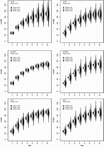
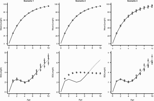
Figure 3. Patterns of among individual variation for a range of values of ψ and a range of among individual variation (CV (k)) and environmental variation (CV (w)). The left column shows the effect of increasing CV (k) for a fixed w and the right column of plots show the effect of increasing CV (w) for a fixed k Each violin plot shows the probability density function of length-at-age for 10,000 simulated individuals. Relatively wider areas indicate lengths with more individuals in the population. All violin plots are scaled by their most abundant length in that age class; violins with larger area do not indicate more individuals, only a wider spread in the observed length-at-age. Shading corresponds to the parameter combination indicated.

We are interested in estimating the following parameters: (1) x ₀, the initial length of individuals; (2) α and β, the parameters controlling fixed individual variation in growth; (3) ψ, a parameter that controls the connection between individual traits and the environment; (4) the vector which has an element for each of the environmental conditions between observed sampling dates; and (5) δ, characterizing the variability of the process stochasicity in growth. In addition, we estimate latent variables at each sampling date which correspond to the mean and variance of length of the population at time t, μ _t , and , respectively.

The distribution of individual lengths does not follow a canonical statistical distribution; the overall shape of the distribution changes as individuals age. The distribution may have stable, increasing, or decreasing variance as the cohort ages and may change over time from left to right skewed (or vice versa). This is evident in Figure 3 where the variance and skew of individual lengths is strongly affected by changing the values of ψ, α , and . We will discuss variation in k and w in terms of the coefficient of variation (CV (k) and CV (w)) instead of α and δ directly. Coefficient of variation is a measure of the amount of variability, relative to the mean with larger CVs indicating more variations.

Given the potential variation in distributional shapes of cohorts, which may range from nearly symmetric to positively (right) skewed, the gamma likelihood provides a flexible distribution for lengths, so we develop statistical methods based on the assumption that the gamma likelihood is an adequate descriptor of length data. Depending on the data that one wishes to analyse, alternate likelihood functions may be desirable and our methods can be implemented by replacing the Gamma likelihood with another likelihood function. Other investigators have found it expedient to describe size-at-age as following a normal or log-normal density 19 48. We address other likelihoods choices and potential alternative methods for estimating parameters in the Discussion.

When analysing a single cohort, t is equivalent to the cohort's age, and we let θ _t and φ _t be the parameters for the gamma distribution describing the distribution of lengths at time t. From the definition of the gamma distribution, these two parameters are determined by the mean (μ _t , Equation (11)) and variance (, Equation (13) of lengths in the population: and . Note that we assume that approximating the distribution of lengths at time point, using the only observed expectation and variance is adequate. We ignore the information contained in the third and higher moments of the observed length distributions.

We let y _{j, t} , represent the length of the jth sampled individual at time t, so \newline ) (bold symbols indicate vectors) is the posterior probability of the parameters and latent variables, given the data, is the prior distribution for the parameters, is the probability of the latent variables given the parameters, and is the likelihood of the data, given the latent variables. The joint posterior of the parameters and latent variables is

This general form provides a fairly flexible structure that provides possible options for more complicated models such as including measurement error or hierarchical structures. Assuming a gamma likelihood, and likelihood of the observed length of individual j at t is

The likelihood of all individuals and sampling times is

In situations when data from multiple cohorts are available, we add a subscript to denote the cohort (c) and the likelihood for all individuals from all cohorts is

To complete the model, we use diffuse, independent priors for all parameters except x ₀ (Table 1); we assume that there is typically very good information on the initial size of individuals in the populations. The option to include prior information about any of the parameters is an important advantage of the Bayesian approach. We use standard Markov chain Monte Carlo (MCMC) approaches to fit the model. We implement all of fitting routines in R (v. 2.13.1 56) and use Metropolis–Hastings MCMC algorithms to estimate the posterior distributions of the parameters 23. We provide details of the fitting algorithms and discuss computational issues in the appendix.

Table 1. Prior distributions for parameters.

Parameter	Prior	Constraints
α	Gamma(0.0001, 0.0001)	α>2
β	Gamma(0.0001, 0.0001)	α>2
γ	Uniform(0, 10000)
δ	Gamma(0.0001, 0.0001)
ψ	Beta(1, 1)	0 1
x 0	Normal(1, 0.0001)	>0

Tests with simulated data

To determine the efficacy of our approach, we tested it against simulated data with known parameters, using three scenarios that demonstrate both the usefulness and potential limitations of our approach. In all simulations, we assume a random sample of lengths are observed from a single cohort of individuals at regularly spaced intervals, to produce a time-series of length-at-age samples. All observations are assumed to be independent samples. We maintain a mean , and mean asymptotic length of an individual with , , in all simulations. In each, we simulated a single cohort of 10,000 individuals using Equation (7) where each individual was assigned a k _i from a Gamma distribution defined at the beginning of the simulation (see Table 2). All individuals started at size x ₀=1 at t=0 and 100 individuals were sampled from at t=1, 2, …, 7.

Table 2. Summary of simulation scenarios.

Parameter	Simulated values	Fixed	Estimated
Scenario 1:
	0.3	–	Yes
CV (k)	0.01, 0.05, 0.10, 0.20	–	Yes
L ∞	100	–	Yes
CV (w)	0.05, 0.10, 0.20	–	Yes
ψ	0, 0.5, 1.0	Yes, ψ=0, 0.5, 1.0
x 0	1	Yes, x 0=1	–
Scenario 2:
	0.3	–	Yes
CV (k)	0.01, 0.05, 0.10, 0.20	–	Yes
L ∞	100	–	Yes
CV (w)	0.05, 0.10, 0.20	–	Yes
ψ	0.25, 0.5, 0.75	Yes, ψ=1	–
x 0	1	Yes, x 0=1	–
Scenario 3:
	0.3	–	Yes
CV (k)	0.01, 0.05, 0.10, 0.20	–	Yes
L ∞	100	–	Yes
CV (w)	0.05, 0.10, 0.20	–	Yes
ψ	0.25, 0.5, 0.75	–	Yes
x 0	1	Yes, x 0=1	–
Notes: Estimated parameters use the prior distributions listed in Table 1. For all scenarios, we scaled the values of γ so that for an individual with , . We also present the variability of k and w in terms of their CV. For k, and for .

In the first scenario, we assume a constant environment for the entire time-series () and that x ₀ and ψ are considered fixed and known. We then estimated α, β, γ, and δ, and the latent variables and from the data. This scenario is comparable in spirit to the most common analysis of growth data where a single growth curve is estimated from a time series of observations. However, our analysis also provides an estimate of the individual variability in k. We compared the ability of our statistical model to estimate parameters used to simulate individuals across a range of individual and stochastic variation by changing CV (k) and CV (w). We performed simulations and estimated parameters from all possible combinations of simulations of four levels of individual variation (, or 0.20) and three levels of environmental stochasticity (, or 0.20). We repeated our simulation and analysis for three values of ψ (ψ=0, 0.5, and 1.0). In total, we simulated 36 parameter combinations (see Table 2). For each parameter combination, we performed three independent simulations and estimated parameters, using MCMC.

In the second scenario, we assume a constant environment for the entire time-series, and that x ₀ is fixed. We simulated populations with three values of ψ (0.25, 0.50, or 0.75), but when fitting the model we assumed ψ=1. Again we estimated α, β, γ, and δ, and the latent variables and from the data. This scenario explores the consequences of assuming a fixed but incorrect value of ψ for the estimates of individual variation in k and is equivalent to asking what are the consequences of assuming that L _∞ is fixed for all individuals when in truth L _∞ varies among individuals 19 54. As in the first scenario, we consider four levels of individual variation and three levels of environmental stochasticity (Table 2).

In the third scenario, we assumed a constant environment γ for the entire time-series and a shared initial size, but considered ψ to be unknown. Thus, we estimated α, β, γ, δ, and ψ and the latent variables from the data. In many ways, this is the most realistic simulation test, because ψ is fitted as a free parameter.

In all cases, we compared the estimates of from our statistical model with the known input parameters for each simulation.

Results

Using simulated data revealed both the value and potential weaknesses of our approach. Across all simulations scenarios, the statistical approach was very good at correctly identifying biological quantites of interest that were combinations of parameters. For example, for all parameter combinations in all three scenarios, the model correctly identified the mean of among individual growth () and the mean asymptotic length () (Figures 4 and A2). The precision of model estimates declined with increased environmental and individual variation, but in all cases the relative error in estimation was very small (always ≤5% ). Also, the model was very good at approximating the length-at-age distributions of ages with sampled individuals and provides good estimates of the distribution of lengths for ages older than those observed (e.g. age 8, 9, or 10; Figure 5).

Figure 4. Estimation bias for and for scenario 1 with ψ=0.5 (see Table 1). In both panels, the dashed line indicates the input value. Point and vertical line indicates a posterior mean and a 90% credible interval for the posterior distribution (50,000 iterations), respectively.

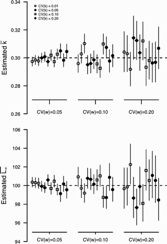
Figure 5. Estimated latent states (mean length-at-age, μ _t (top row) and standard deviation of length-at-age, σ _t (bottom row)) for three statistical models (columns). The true underlying mean and standard deviation are indicated by the line. For each scenario, parameters were estimated for three independent simulations (points: mean posterior estimate±1 standard error derived from 1000 posterior samples). Points have been slightly jittered along the x-axis to reduce overlap. For all scenarios, individuals were simulated using CV(k)=0.2 and CV(w)=0.05 (see Table 2 and methods for full scenario descriptions). The solid line indicates the range of age for which individuals were observed (ages 1–7). The dashed line indicates ages for which no sampled lengths were included in the fitting procedure (ages 8–10). Note that the statistical model provides estimates for the mean and variance beyond the range of observed ages.

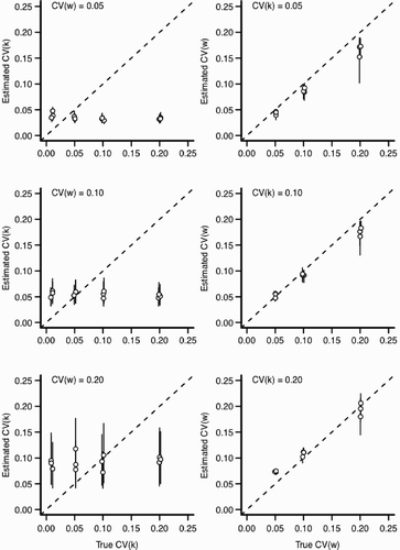
However, the ability to identify the primary parameters of interest (the individual variability in growth rate, CV (k), and environmental variation, CV (w), varies according to the scenario. When we assumed that ψ was known without error (Scenario 1), the statistical model estimated both CV (k) and CV (w) well (Figure 6). For scenario 1, the only situation in which the model performed poorly was when individual variation was very small . For small CV (k), the model tends to overestimate the amount of individual variation. Estimation bias increased with the amount of variation in the environment (CV (w); Figure 6). While this pattern of relative bias held true across all three values of ψ considered, the relative error in the estimated parameters was much larger for ψ=0.5 than ψ=0 or 1 (compare Figure 6 with Figure A4). In particular, the statistical model had difficultly identifying CV (k) under simulations with large environmental stochasticity . The cause of a poor model performance is likely explained by strong similarity between distribution of length-at-age across a range of CV (k) (see Figure 3 with ψ=0.5). There are many values of CV (k) that generate very similar distributions of length-at-age and there is simply insufficient information contained in the distribution of lengths to distinguish among possible values of CV (k). This fact is magnified when there is a large amount of environmental variation that produces an especially broad distribution of length-at-age. This problem will decline with increased sample sizes as estimates of the length-at-age distribution improve. An additional contributor to parameter mis-estimation is likely our assumption that the distribution of lengths follows a gamma density (Figure 7). For ψ=0.5, changing CV (k) has a relatively small effect on the variance in length-at-age distribution (Figure 3), but does affect the skew of length-at-age; the skew becomes more negative as CV (k) and CV (w) increase (see also Figure 7). As implemented with the Gamma likelihood, we cannot properly account for the left skewed length-at-age distributions and have some difficultly estimating the underlying parameters. In this case, attempts to fit the model using other likelihood functions including the normal likelihood performed similarly.

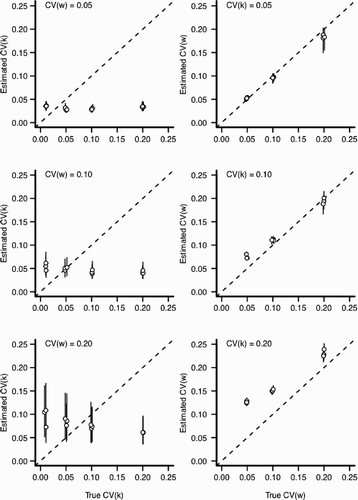
Figure 6. Estimation bias for individual and environmental variation for scenario 1 with ψ=0 (see Table 1). In all panels, x-axis indicates the value input into the simulation and y-axis indicates the estimated value from the statistical model. Perfect estimation would be indicated by points lying upon the dashed line. Each point and vertical line indicates a posterior mean and a 90% credible interval for the posterior distribution, respectively. Points have been slightly jittered along the x-axis to reduce overlap. Left column: The effect of increasing environmental variation (CV (w)) for the estimation of CV (k). Right column: The effect of increasing individual variation (CV (k)) for the estimation of CV (w).

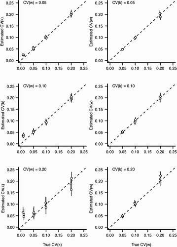
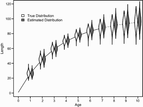
Figure 7. Length-at-age distributions for 10,000 simulated individuals (‘true’) and estimated posterior distribution from scenario 3 with CV(k)=0.2 and CV(w)=0.05 (see Table 2). The solid line indicates the mean length-at-age of observed individuals (ages 1–7), while the dashed line indicates the mean length-at-age for which no sampled lengths were included (ages 8–10). For a description of violin plots see Figure 2.

Assuming a specific but incorrect value of ψ during model fitting (scenario 2) yielded incorrect inference about the amount of individual versus environmental variation in populations. When the model is mis-specified (assuming ψ=1 when ψ≠1), the statistical model tends to overestimate the contribution of environmental variation and estimate a consistent amount of individual variation regardless of the true value of CV (k) (Figures 8 and A5). That parameter estimates derived from an incorrect statistical model are biased is not particularly surprising. However, the direction and magnitude of the estimation bias are substantial and were not obvious before we fit the model. This result is a general caution against fitting complex growth models with many parameters by assuming some parameters are fixed and known when they are not; an approach commonly undertaken when authors use parameter-rich physiological models to estimate individual variation and only allow a few parameters to be estimated from the data 30. If the assumptions are correct, the inference is entirely valid. However, if the parameters are fixed at an incorrect value, the estimates for unknown parameters will be strongly biased and, potentially, misleadingly precise (Figures 8 and A5). Even with a mis-specified value of ψ, the estimated mean of length-at-age matched the true mean very well (Figure 5; see 19). However, the estimated variance substantially differed from the true variance-at-age (Figure 5)

Figure 8. Estimation bias for individual and environmental variation for scenario 2 with ψ=0.25 but fit assuming ψ=1 (see Table 1). In all panels, x-axis indicates the value input into the simulation and y-axis indicates the estimated value from the statistical model. Perfect estimation would be indicated by points lying upon the dashed line. Each point and vertical line indicates a posterior mean and a 90% credible interval for an independent MCMC sampler (50,000 iterations), respectively. Points have been slightly jittered along the x-axis to reduce overlap. Left column: The effect of increasing environmental variation (CV (w)) for the estimation of CV (k). Right column: The effect of increasing individual variation (CV (k)) for the estimation of CV (w).

Estimating parameters for scenario 3 proved to be more difficult than in the other scenarios. because the posterior samples of γ and ψ in the MCMC chain were strongly correlated. In some cases, the covariation of parameters either prevented the model from converging to a posterior distribution or the mixing of the posterior chains was poor enough to make determination of convergence of the model uncertain. In others scenarios, the MCMC sampler clearly converged but produced posterior chains that mixed poorly with high autocorrelation. Poorly mixing chains required long simulations (several hundred thousand iterations) to obtain meaningful parameter estimates. This occurred despite a substantial amount of effort to design and implement efficient mixing in the MCMC (see Appendix) and arises primarily because of the model formulation: γ and ψ both occur in the same term in the growth equation (see Equation (7)). Therefore, estimates of the parameters are strongly correlated. Despite these problems, scenario 3 provided good estimates of parameters that were combinations of parameters (e.g. and ; Figure A3). Even when γ and ψ mixed poorly, the marginal posteriors for and converge near the true values (Figure A3). Similarly, the mean and variation of length-at-age from the latent variables tend to converge and mix reasonably well. For example, Figures 5 and 7 compare latent variable estimates to true values from one simulation scenario that converged and mixed well. Generally, the statistical model tended to converge successfully when individual variation in k was substantial (CV(k)=0.10 or 0.20) and similar or larger than the magnitude of environmental variation (CV). But we view the resulting estimates of CV (k) and CV (w) to be uncertain to allow any discussion of general patterns of the estimation bias or precision.

Anecdotally, increasing the sample size of individuals improved the mixing properties of all posterior simulations. Sampled lengths from old individuals who were near the asymptotic length were particularly influential in improving the estimation of parameters.

Discussion

Our formulation of the VBGF – which is a balance of biological detail and statistical rigour – provides a flexible approach to understanding the interaction between behavioural traits, intrinsic individual variation and environmental variation and how these factors combine to affect growth. Our work provides analytic solutions for the expectation and variance of length-at-age, given model parameters and a statistical framework for estimating model parameters. As written, our model is directly applicable to instances in which it can be assumed that growth is the only factor driving variation among individuals. Thus, the approach presented here is directly applicable to populations for which other size-dependent processes such as mortality can be reasonably assumed to be negligible. In the presence of size-dependent mortality, it may be quite difficult to estimate individual variation 7 48. Explicitly accounting for other processes such as size-dependent mortality can be added to the model presented, but incorporating such processes is beyond the scope of this paper.

We used simulated data to identify both strengths and weaknesses of the statistical methodology. In all simulation scenarios, the model provided accurate estimates of and , as well as descriptions of the distribution of length-at-age (Figures 4 and 5). Our results parallel the conclusions reached by Eveson et al. 19 who assessed the efficacy of several models to estimate mean length-at-age when individual variation in k and/or L _∞ was assumed. They showed that treating k and/or L _∞ as varying among individuals, even when these assumptions were incorrect, produced less biased estimates of the mean length-at-age.

We move beyond their work by incorporating information from the variance of the distribution of length to estimate the amount of individual variation in the population. Estimating individual variation from observational population samples is difficult and can be prone to error (Figures 6 and 8), and in some cases (scenario 3), subject to statistical computing challenges. However, there is cause for optimism: estimating individual variation using reasonable sample sizes and widely available data sources is possible.

Our results indicate that using statistical methods based on only the first two moments of size-at-age distributions are sufficient to estimate both individual and environmental variation. The performance of the parameter estimation algorithm for the full model (scenario 3) clearly indicates that some statistical challenges remain. Additional information improved the model performance. Specifying the value of ψ (scenario 1) resulted in good estimation in most instances. However, it seems unlikely that ψ can be specified a priori in most cases and scenario 2 illustrates the consequences of fixing ψ at an incorrect value (Figure 8).

There are at least three accessible sources for additional information about individual variation that should improve the estimation of parameters in scenario 3. First, and most obviously, larger sample sizes of length-at-age improve model performance. Second, informative prior distributions for any parameters, but for γ and ψ in particular would increase model identifiability. Prior information could potentially come from mark-recapture data of the growth of individuals or an understanding of behavioural biology. Different sources of prior information pose practical challenges, but the Bayesian framework developed here present a way to integrate diverse data sources to understand the process of growth.

A third and perhaps a more readily available source of information is from the length-at-age data itself. Our analytical solutions provide expressions for the mean and variance of length in the population as a function of the parameters. In using only the mean and the variance, we ignore the information contained in the higher moments of the distribution of length-at-age. However, different combinations of parameters can generate length-at-age distributions that are not symmetric – some are left skewed while others are right skewed (Figure 3). Since skew is associated with the third moment of distribution, it is logical that including information from the third moment might aid parameter identifiability. This aspect of our model does cause some mismatch between estimated and true length-at-age (see Figure 7) because the gamma likelihood cannot account for negative skew. At present, developing methods that can include information from the the third and higher moments is a non-trivial statistical task that warrants future investigation (see also the appendix).

The methods outlined here emphasize the value of moving beyond the mean length-at-age for investigating individual variation in growth. Many models can provide adequate descriptions of the mean length-at-age (Figure 5; see also 19 53), but most growth models do not compare the variance of lengths in the data and the model. Mis-specifying the growth model can result in good estimates of the mean length-at-age, but a mismatch between the estimated and true variance of the length-at-age (Figure 5). A current avenue of research is determining how to incorporate the information contained in the third moment (and, potentially, quantities related to higher moments) for the inference of biological parameters. We speculate that moving from a likelihood framework towards a Generalized Method of the Moments framework may be a way to advance estimation of individual variation 76. Other possibilities include using synthetic likelihood approaches 75 or Approximate Bayesian Computation methods 12. All three approaches can be employed to exploit the information contained in the higher moments of the length-at-age distribution. None of these approaches are widely known or implemented in the ecological literature currently and the development of statistical methods based on these approaches are difficult. However, such approaches do suggest that there is hope for extracting additional biological details from observational time-series of individuals.

In all of our simulation scenarios, we assumed fairly simple biological scenario: a single cohort of individuals growing in a constant environment. With a single cohort of fish, estimating multiple environmental states in concert with the other parameters is not possible; length data from multiple cohorts observed in a single year are required to estimate discrete environments. In the future, our model should be tested against more realistic situations with multiple co-occuring cohorts and a variable environment. Describing the environment as a function of environmental covariates 36 would likely increase the identifiability of environmental parameters. As an aside, the simultaneous analysis of multiple cohorts may allow improved estimation of ψ as well.

Beyond our ability to statistically estimate the parameters, the model for growth provides a forum for investigating topics such as growth autocorrelation where certain individuals grow faster than others 50 51. Population level data will never provide the same amount of biological insight as that which is available from individual tagging data. However, individual-level tagging data are difficult to collect while simple population censuses are relatively easy. The Bayesian framework provides a direct method for incorporating analyses from individual level data with observational data and provides intuitive ways to make predictions about the length-at-age distributions.

Acknowledgements

This work was supported by the Center for Stock Assessment Research, a partnership between the Fisheries Ecology Division, NOAA Fisheries, Santa Cruz, CA and the University of California Santa Cruz and by NSF grant EF-0924195 to MM. We thank E.J. Dick, S. Munch, W. Satterthwaite, and S. Vincenzi for helpful discussions and comments on the manuscript

Notes

Throughout the paper, we use Gamma densities of the form, , where Γ is the Gamma function. The Gamma density has an expected value, , variance, , and a coefficient of variation, .

Appendix

Analytical expression for variance with among individual variability in k and q

In the main text, we derived expressions for the expected value of length-at-age when k and q are independent but vary among individuals (Equations (4) and (5)). Here we derive the general expression for variance of length-at-age. Using the definition of variance, , an initial size for all individuals x ₀ and assuming that q is normally distributed among individuals, ,

where E[x(t)] is given by Equation (5). Completing this double integration yields

MCMC implementation details

Sampling from the posterior distribution

In this section, we describe the technical details of the Metropolis–Hastings MCMC sampler.

Conditional posterior distributions

We present only the statistical details for sampling from the posterior distribution of Scenario 3 since Scenarios 1 and 2 are special cases of Scenario 3. From Equation (17) in the main text, the joint posterior for the parameters and latent variables is

We sample from the joint posterior by sequentially sampling from the conditional posterior distributions for the parameters and latent variables. Bold indicates vectors and for parameters that are constant in each equation have been omitted on the right side of each equation for notational simplicity.

The latent variables, and , are deterministic functions of the lower level parameters, so we do not need to sample them. Note that we update α and β in one step. After specifying the prior distributions for the parameters, we use standard MCMC sampling techniques for these posterior distributions.

Proposal distributions

An integral part of efficiently sampling from the posterior distribution is developing efficient proposal distributions for the parameters. To sample the posterior, we performed independent, sequential MCMC chains for each data set. For the first MCMC chain, we used independent, normally distributed proposal distributions. We discovered that mixing of α, β, δ, was greatly improved using log-normal proposal distributions. Thus, for example, a proposed value of δ, δ*, would be , where δ _c is the current value of δ and is the proposal variance on the log scale. Because log-normal proposal distributions are asymmetric, we had to include a term in the acceptance step of the Metropolis–Hastings algorithm that accounts for this asymmetry 23. We use normal proposal distributions for ψ and γ.

In most situations, ψ had unreasonably low acceptance rates so we used adaptive sampling approaches to modify the proposal distribution for ψ until its acceptance rate ranged from 0.2 to 0.4. We ran this first MCMC for 10,000–20,000 iterations and used the accepted values from the burn-in MCMC to calculate an empirical variance–covariance matrix for the parameters α, β, , and δ. Then we used this variance–covariance matrix for the multivariate normal proposal distributions in the second MCMC. For scenarios 1 and 2, we used this second MCMC as our final sampler. For scenario 3, we used a third MCMC that used a variance–covariance matrix from accepted values from the second MCMC as the proposal distribution for the third MCMC. For the parameters with normal proposal distributions, we rejected proposed negative values or values outside of the possible range of that parameter.

Initially, we used trace plots of the MCMC chain to assess convergence of all parameters. In addition, we used Geweke criteria to compare the variance of the first 10% of samples in the final chain to the last 50% of samples to confirm convergence.

Analytical solution for the skew of the distribution of lengths

It is possible to derive analytic expressions for quantities associated with higher moments of the distribution as well. Here we derive the general expression for the skew of the distribution of length-at-age (which is associated with the third moment of the distribution). By definition, , where E[X(t)³] is the unnormalized third moment of the distribution of lengths, and μ and σ² are given by Equations (14) and (16), respectively. Thus, we need to evaluate E[X(t)³], where

This integral is available in the closed form, but the expression is complicated and so we leave its evaluation to interested parties.

Figure A1. Expected growth trajectories for three individuals with fixed differences in q (q=11, 10, or 9) but identical k (k=0.10). All individuals were assumed to have a starting length of 1 and live in a constant environment. The x-intercept of each line corresponds to an individuals expected asymptotic length, L _∞.

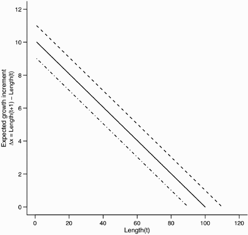
Figure A2. Estimation bias for and for scenario 2 with ψ=0.50 but fit assuming ψ=1 (see Table 1). In both panels, dashed line indicates the input value. Point and vertical line indicates a posterior mean and a 90% credible interval for the posterior distribution, respectively.

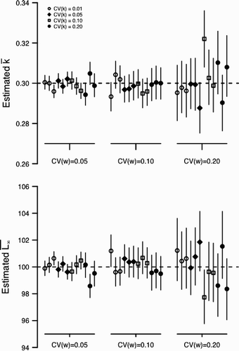
Figure A3. Estimation bias for and for scenario 3 with a simulated, true value of ψ=0.50. ψ estimated as a free parameter (see Table 1). In both panels, dashed line indicates the input value. Point and vertical line indicates a posterior mean and a 90% credible interval for the posterior distribution, respectively.

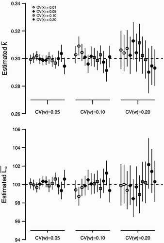
Figure A4. Estimation bias for individual and environmental variation for scenario 1 with ψ=0.5 (see Table 1). In all panels, the x-axis indicates the value input into the simulation and the y-axis indicates the estimated value from the statistical model. Perfect estimation would be indicated by points lying upon the dashed line. Each point and the vertical line indicate a posterior mean and 90% credible interval for an independent MCMC sampler (50,000 iterations), respectively. Points have been slightly jittered along the x-axis to reduce overlap. Left column: The effect of increasing environmental variation (CV (w)) for the estimation of CV (k). Right column: The effect of increasing the individual variation (CV (k)) for the estimation of CV (w).

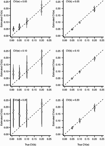
Figure A5. Estimation bias for individual and environmental variation for scenario 2 with ψ=0.50 but fit assuming ψ=1 (see Table 1). In all panels, the x-axis indicates the value input into the simulation and the y-axis indicates the estimated value from the statistical model. Perfect estimation would be indicated by points lying upon the dashed line. Each point and the vertical line indicate a posterior mean and a 90% credible interval for an independent MCMC sampler (50,000 iterations), respectively. Points have been slightly jittered along the x-axis to reduce overlap. Left column: The effect of increasing environmental variation (CV (w)) for the estimation of CV (k). Right column: The effect of increasing individual variation (CV (k)) for the estimation of CV (w).

References

- Alonzo , S. H. , Switzer , P. V. and Mangel , M. 2003 . An ecosystem-based approach to management: Using individual behaviour to predict indirect effects of Antarctic krill fisheries on penguin foraging . J. Appl. Ecol. , 40 : 692 – 697 .
- von Bertalanffy , L. 1938 . A quantitative theory of organic growth (inquiries on growth laws. II) . Human Biol. , 10 : 181 – 213 .
- Beverton , R. J.H. and Holt , S. J. 1957 . On the dynamics of exploited fish populations . UK Min. Agric. Fish. Fish. Invest. , 19 : 97 – 105 .
- von Bertalanffy , L. 1957 . Quantitative laws in metabolism and growth . Quart. Rev. Biol. , 32 : 217 – 231 .
- Bjørnstad , O. N. and Hansen , T. F. 1994 . Individual variation and population dynamics . Oikos , 69 : 167 – 171 .
- Candy , S. and Kawaguchi , S. 2006 . Modelling growth of antarctic krill. II. Novel approach to describing the growth trajectory . Mar. Ecol. Prog. Ser. , 306 : 17 – 30 .
- Carlson , S. , Kottas , A. and Mangel , M. 2010 . Bayesian analysis of size-dependent over-winter mortality from size-frequency distributions . Ecology , 91 : 1016 – 1024 .
- Clutton-Brock , T. and Sheldon , B. C. 2010 . Individuals and populations: The role of long-term, individual-based studies of animals in ecology and evolutionary biology . Tren. Ecol. Evol. , 25 : 562 – 573 .
- Connover , D. O. and Munch , S. B. 2002 . Sustaining fisheries yields over evolutionary time scales . Science , 297 : 94 – 96 .
- Coulson , T. , Benton , T. G. , Lundberg , P. , Dall , S. R.X. , Kendall , B. E. and Gaillard , J.-M. 2006 . Estimating individual contributions to population growth: Evolutionary fitness in ecological time . Proc. R. Soc. Lond. B. Biol. , 273 : 547 – 556 .
- Cressie , N. and Wikle , C. K. 2011 . Statistics for Spatial-Temporal Data , New York : John Wiley and Sons .
- Csilléry , K. , Blum , M. G.B. , Gaggiotti , O. E. and Frano¸is , O. 2010 . Approximate bayesian computation (ABC) in practice . Trends Ecol. Evol. , 25 : 410 – 418 .
- Darimont , C. T. , Carlson , S. M. , Kinnison , M. T. , Paquete , P. C. , Reimchen , T. E. and Wilmers , C. C. 2009 . Human predators outpace other agents of trait change in the wild . Proc. Natl. Acad. Sci. USA , 106 : 952 – 954 .
- DeAngelis , D. L. and Mooij , W. M. 2005 . Individual-based modeling of ecological and evolutionary processes . Ann. Rev. Ecol. Evol. Syst. , 36 : 147 – 168 .
- DeAngelis , D. L. , Rose , K. A. , Crowder , L. B. , Marschall , E. A. and Lika , D. 1993 . Fish cohort dynamics: Application of complementary modeling approaches . Am. Nat. , 142 : 604 – 622 .
- DeGroot , M. H. 1970 . Optimal Statistical Decisions , New York : McGraw Hill .
- Deriso , R. B. and Parma , A. M. 1988 . Dynamics of age and size for a stochastic population model . Can. J. Fish. Aquat. Sci. , 45 : 1054 – 1068 .
- Essington , T. E. , Kitchell , J. F. and Walters , C. J. 2001 . The von Bertalanffy growth function, bioenergetics, and the consumption rates of fish . Can. J. Fish. Aquat. Sci. , 58 : 2129 – 2138 .
- Eveson , J. P. , Polacheck , T. and Laslett , G. M. 2007 . Consequences of assuming an incorrect error structure in von Bertalanffy growth models: A simulation study . Can. J. Fish. Aquat. Sci. , 64 : 602 – 617 .
- Fabens , A. J. 1965 . Properties and fitting of the von Bertalanffy growth curve . Growth , 29 : 265 – 289 .
- Francis , R. I.C.C. 1988 . Maximum likelihood estimation of growth and growth variability from tagging data . New Zealand J. Mar. Fresh. Res. , 22 : 42 – 51 .
- Fujiwara , M. , Kendall , B. E. and Nisbet , R. M. 2004 . Growth autocorrelation and animal size variation . Ecol. Lett. , 7 : 106 – 113 .
- Gelman , A. , Carlin , J. B. , Stern , H. S. and Rubin , D. B. 2004 . Bayesian Data Analysis , 2 , Boca Raton , FL : Chapman & Hall/CRC Press .
- Grant , P. R. and Grant , B. R. 2002 . Unpredictable evolution in a 30-year study of Darwin's finches . Science , 296 : 707 – 711 .
- Grimm , V. and Uchmanski , J. 2002 . Individual variability and population regulation: A model of the significance of within-generation density dependence . Oecologia , 131 : 196 – 220 .
- Gross , M. R. 1991 . Evolution of alternative reproductive strategies: Frequency-dependent sexual selection in male bluegill sunfish . Philos. Trans. R. Soc. Biol. Sci. , 332 : 59 – 66 .
- Gudmundsson , G. 2005 . Stochastic growth . Can. J. Fish. Aquat. Sci. , 62 : 1746 – 1755 .
- Hare , J. A. and Cowen , R. K. 1997 . Size, growth, development, and survival of the planktonic larvae of Pomatomus saltatrix (Pisces: Pomatomidae) . Ecology , 78 : 2415 – 2431 .
- Harper , J. L. 1977 . The Population Biology of Plants , London : Academic Press .
- Harvey , C. J. 2009 . Effects of temperature change on demersal fishes in the California Current: A bioenergetics approach . Can. J. Fish. Aquat. Sci. , 66 : 1449 – 1461 .
- He , J. X. and Bence , J. R. 2007 . Modeling annual growth variation using a hierarchical Bayesian approach and the von Bertalanffy growth function, with application to lake trout in souther Lake Huron . Trans. Amer. Fish. Soc. , 136 : 318 – 330 .
- Helser , T. E. and Lai , H. L. 2004 . A Bayesian hierarchical meta-analysis of fish growth: With an example for North American largemouth bass, Micropterus salmoides . Ecol. Mod. , 178 : 399 – 416 .
- Helser , T. E. , Stewart , I. J. and Lai , H.-L. 2007 . A Bayesian hierarchical meta-analysis of growth for the genus Sebastes in the eastern Pacific Ocean . Can. J. Fish. Aquat. Sci. , 64 : 470 – 485 .
- Kawaguchi , S. , Candy , S. , King , R. , Naganobu , M. and Nicol , S. 2006 . Modelling growth of Antarctic Krill. I. Growth trends with sex, length, season, and region . Mar. Ecol. Prog. Ser. , 306 : 1 – 15 .
- Kawaguchi , S. , Yoshida , T. , Finley , L. , Cramp , P. and Nicol , S. 2007 . The krill maturity cycle: A conceptual model of the seasonal cycle in Antarctic krill . Polar Biol. , 30 : 689 – 698 .
- Kimura , D. K. 2008 . Extending the von Bertalanffy growth model using explanatory variables . CJFAS , 65 : 1879 – 1891 .
- Kitchell , J. F. , Stewart , D. J. and Weininger , D. 1977 . Applications of a bioenergetics model to yellow perch (Perca flaescens) and walleye (Stizostedion vitreum vitreum) . J. Fish. Res. Board Can. , 34 : 1922 – 1935 .
- Knape , J. , Jonzen , N. , Skold , M. , Kikkawa , J. and McCallum , H. 2011 . Individual heterogeneity and senescence in Silvereyes on Heron Island . Ecology , 92 : 813 – 820 .
- Kooijman , S. A.L.M. 2000 . Dynamic Energy and Mass Budgets in Biological Systems , 2 , Cambridge : Cambridge University Press .
- Koskella , B. and Lively , C. M. 2009 . Evidence for negative frequency-dependent selection during experimental coevoluation of a freshwater snail and a sterilizing trematode . Evolution , 63 : 2213 – 2221 .
- Kruuk , L. E. 2004 . Estimating genetic parameters in natural populations using the ‘animal model’ . Phil. Trans. Roy. Soc. B , 359 : 873 – 890 .
- Laslett , G. M. , Eveson , J. P. and Polacheck , T. 2002 . A flexible maximum likelihood approach for fitting growth curves to tag-recapture . Can. J. Fish. Aquat. Sci. , 59 : 976 – 986 .
- Magnuson , J. J. 1962 . An analysis of aggressive behavior, growth, and competition for food and space in Medaka (Oryzias latipes (Pisces, Cyprinodontidae)) . Can. J. Zool. , 40 : 313 – 363 .
- Mangel , M. 2006 . The Theoretical Biologist's Toolbox , Cambridge : Cambridge University Press .
- Metcalfe , N. B. , Taylor , A. C. and Thorpe , J. E. 1995 . Metabolic rate, social status and life-history strategies in Atlantic salmon . Anim. Behav. , 49 : 431 – 436 .
- Nisbet , R. M. , Muller , E. B. , Lika , K. and Kooijman , S. A.L.M. 2000 . From molecules to ecosystems through dynamic energy budget models . J. Anim. Ecol. , 69 : 913 – 926 .
- Palmer , A. R. 1984 . Prey selection by thaidid gastropods: some observational and experimental field tests of foraging models . Oecologia , 62 : 162 – 172 .
- Parma , A. M. and Deriso , R. B. 1990 . Dynamics of age and size composition in a population subject to size-selective mortality: Effects of phenotypic variability in growth . Can. J. Fish. Aquat. Sci. , 47 : 274 – 289 .
- Paszkowski , C. A. and Olla , B. L. 1985 . Social interaction of coho salmon (Oncorhynchus kisutch) smolts in seawater . Can. J. Zool. , 63 : 2401 – 2407 .
- Pfister , C. A. and Stevens , F. R. 2002 . Genesis of size variability in plants and animals . Ecology , 83 : 59 – 72 .
- Pfister , C. A. and Stevens , F. R. 2003 . Individual variation and environmental stochasticity: Implications for matrix model predictions . Ecology , 84 : 496 – 510 .
- Pfister , C. A. and Wang , M. 2005 . Beyond size: Matrix projection models for populations where size is an incomplete descriptor . Ecology , 86 : 2673 – 2683 .
- Pilling , G. M. , Kirkwood , G. P. and Walker , S. G. 2002 . An improved method for estimating individual growth variability in fish, and the correlation between von Bertalanffy growth parameters . Can. J. Fish. Aquat. Sci. , 59 : 424 – 432 .
- Punt , A. E. , Hobday , D. , Gerhard , J. and Troynikov , V. S. 2006 . Modelling growth of rock lobsters, Jasus edwardsii, off Victoria, Australia using models that allow for individual variation in growth parameters . Fish. Res. , 82 : 119 – 130 .
- Quinn , T. P. and Deriso , R. 1999 . Quantitative Fish Dynamics , Oxford : Oxford University Press .
- R Development Core Team . R: A Language and Environment for Statistical Computing R Foundation for Statistical Computing, Vienna, Austria, 2011, ISBN 3-900051-07-0. Available at http://www.R-project.org.
- Rice , J. A. , Miller , T. J. , Rose , K. A. , Crowder , L. B. , Marschall , E. A. , Trebitz , A. S. and DeAngelis , D. L. 1993 . Growth rate variation and larval survival: Inferences from an individual-based size-dependent predation model . Can. J. Fish. Aq. Sci. , 50 : 133 – 142 .
- Ricker , W. E. 1958 . Handbook of computations for biological statistics of fish populations . Fish. Res. Bd. Canada , Bulletin Number 119.
- Ryer , C. H. and Olla , B. L. 1996 . Growth depensation and aggression in laboratory reared coho salmon: The effect of food distribution and ration size . J. Fish Biol. , 48 : 686 – 694 .
- Sainsbury , K. J. 1980 . Effect of individual variability on the von Bertalanffy growth equation . Can. J. Fish. Aquat. Sci. , 37 : 241 – 247 .
- Schmitt , J. , Eccleston , J. and Ehrhardt , D. W. 1987 . Dominance and suppression, size-dependent growth and self thinning in a natural Impatiens capensis population . J. Ecol. , 75 : 651 – 665 .
- Schmitt , J. , Ehrhardt , D. W. and Cheo , M. 1986 . Light-dependent dominance and suppression in experimental radish populations . Ecology , 67 : 1502 – 1507 .
- Siegfried , K. I. and Sanso , B. 2006 . Two Bayesian methods for estimating parameters of the von Bertalanffy growth equation . Environ. Biol. Fish. , 77 : 301 – 308 .
- Snover , M. L. , Watters , G. M. and Mangel , M. 2005 . Interacting effects of behavior and oceanography on growth in salmonids with examples for coho salmon (Oncorhynchus kisutch) . Can. J. Fish. Aquat. Sci. , 62 : 1219 – 1230 .
- Snover , M. L. , Watters , G. M. and Mangel , M. 2006 . Top-down and bottom-up control of life history strategies in coho salmon (Oncorhynchus kisutch) . Am. Nat. , 167 : E140 – E157 .
- Stopher , K. V. , Pemberton , J. M. , Clutton-Brock , T. H. and Coulson , T. 2008 . Individual differences, density dependence and offspring birth traits in a population of red deer . Proc. Roy. Soc. B. , 275 : 2137 – 2145 .
- Tinker , M. T. , Bentall , G. and Estes , J. A. 2008 . Food limitation leads to behavioral diversification and dietary specialization in sea otters . Proc. Nat. Acad. Soc. USA , 105 : 560 – 565 .
- Troynikov , V. S. 1998 . Probability density functions useful for parametrization of heterogeneity in growth and allometry data . Bull. Math. Biol. , 60 : 1099 – 1122 .
- Vindenes , Y. , Engen , S. and Saether , B.-E. 2008 . Individual heterogeneity in vital parameters and demographic stochasticity . Am. Nat. , 171 : 455 – 467 .
- Wang , Y.-G. 1998 . Effect of individual variability on estimation of population parameters from length-frequency data . Can. J. Fish. Aquat. Sci. , 55 : 2393 – 2401 .
- Wang , Y.-G. , Thomas , M. R. and Somers , I. F. 1995 . A maximum likelihood approach for estimating growth from tag-recapture data . Can. J. Fish. Aquat. Sci. , 52 : 252 – 259 .
- Weiner , J. 1985 . Size hierarchies in experimental populations of annual plants . Ecology , 66 : 743 – 752 .
- West , L. 1986 . Interdividual variation in prey selection by the snail Nucella (=Thais) emarginata . Ecology , 67 : 789 – 809 .
- Wiedenmann , J. , Creswell , K. and Mangel , M. 2008 . Temperature-dependent growth of Antarctic krill: Predictions for a changing climate from a cohort model . Mar. Ecol. Prog. Ser. , 358 : 191 – 202 .
- Wood , S. N. 2010 . Statistical inference for noisy nonlinear ecological dynamic systems . Nature , 466 : 1102 – 1104 .
- Yin , G. 2009 . Bayesian generalized method of moments . Bayesian Anal. , 4 : 191 – 208 .