General Allee effect in two-species population biology

Abstract

The main objective of this work is to present a general framework for the notion of the strong Allee effect in population models, including competition, mutualistic, and predator–prey models. The study is restricted to the strong Allee effect caused by an inter-specific interaction. The main feature of the strong Allee effect is that the extinction equilibrium is an attractor. We show how a ‘phase space core’ of three or four equilibria is sufficient to describe the essential dynamics of the interaction between two species that are prone to the Allee effect. We will introduce the notion of semistability in planar systems. Finally, we show how the presence of semistable equilibria increases the number of possible Allee effect cores.

Keywords:

• population biology
• competition models
• Allee effect
• semistability
• extinction region

1. Introduction

In their book, Courchamp et al. 4, the authors described the Allee effect in a straightforward manner: ‘The more the merrier: This effect is simply a causal positive relationship between the number of individuals in a population and their fitness. The more individuals there are (up to a point), the better they fare’. So as population size approaches a threshold, favourable influences stimulate its growth and when it goes below it, unfavourable influences inhibit its growth. From their point of view, the Allee effect may be described as a notion of positive density dependence in which ‘the overall individual fitness, or one of its components, is positively related to population size or density’ 4. However, Lidicker 15 recently proposed that Allee effects may be described and defined in terms of demographic processes. He explained that ‘Allee effects are expressed at the population level of organization, and the parameters of interest are the population properties of growth rates, recruitment rates, loss rates, equilibrium densities, and perhaps, success in establishing new populations’. All the above authors indicated that they are using size and density interchangeably, unless otherwise explicitly stated.

Allee et al. 1 2 provided experimental and field studies that confirmed the presence of the Allee effect among many species. The examples include bobwhite quails (Colinus virginianus) that huddle together to lower the surface presented to cold weather, and the disappearance of tsetse fly from an area in which the density of the flies fall below a threshold minimum density (see also 11,13–16,19 20).

Let x _n denote the size or density of species x at the time period or generation n. Then, we define the fitness of species x as the per-capita growth of its population, represented by the function . Thus, the difference equation that models the growth of the population is given by

Definition Model (1) is said to have a strong Allee effect if the following conditions hold true:

	(1)  for for some ,
	(2) f(0)<1,
	(3) There exists a unique K>0, such that f(K)=1, .

Remark

It follows from the above conditions that there exists a fixed point A, 0<A<K, such that f(A)=1 and A is unstable.

In the absence of the Allee effect, the fitness is expected to decrease when the population increases, most likely as the result of inter-specific competition, difficulty in finding mates, or/and limitation of resources. On the other hand, a strong Allee effect is exhibited by an increase in per-capita growth with increasing population size. These competing mechanisms can be readily modelled for a single species x as follows. The fitness of the population is represented by the product

where , ; f ₀(x) is the fitness function if there is no Allee effect, and I(x) represents the Allee effect on the fitness of the population. The assumption ensures the negative correlation of the fitness with the population size (in the absence of the Allee effect), i.e. the fitness decreases when the population increases (negative density dependence). On the other hand, produces the required dynamics of the Allee effect that may lead to extinction of the population if it falls below a certain threshold (positive density dependence).

An example of a model having the dynamics of (2) is the λ-Ricker Map 11,

where and , λ>1. The physical meaning of the exponent λ in Equation (3) is given by the percentage rate of change as follows:

This may be easily shown by taking the derivative of Equation (3) near the fixed point x=0, i.e. and then dividing this by Equation (3), where we obtain .

For two-species models representing two species x and y, the difference equation is given by the planar system

General planar models with the Allee effect caused by an inter-specific interaction may be written in a form extending Equation (2) to two-species model,

Furthermore, by extending the Λ-Ricker model to two species, we obtain the following planar system:

with x _n >0, y _n >0 and Λ₁, Λ₂>0.

For the suitable selection of the parameters there can be up to seven fixed points:

•	Origin: (0, 0).
•	Two fixed points on the x-axis, given implicitly by the roots of , when .
•	Two fixed points on the y-axis, again given implicitly by , when .
•	Two fixed points in the interior, given by the system and . In the case of a symmetric model, i.e. , , , , two fixed points exist in the interior, if .

Another interesting example of a planar model that describes a two-species competition model exhibiting contest inter-specific competition 18 is the following 10:

with . This model may have up to nine fixed points:

•	Origin: (0, 0).
•	Two fixed points on the x-axis,
•	Two fixed points on the y-axis,
•	Four fixed points in the interior. We can easily compute these fixed points for the symmetric case, where and . They are given by , for a>b+2, and , , for .

Next, we will introduce the notion of semistability in planar systems.

2. Semistability

Let us start by defining the notion of semistability in the one-dimensional case.

Definition A fixed point x* is said to be semistable if there exists an interval , , such that x* is attracting from one side and repelling from the other side. It is said to be semistable from the left {right} if it is attracting on .

We will start our exposition by stating the main result of semistability for single species (one-dimensional maps).

Theorem 1

6 Consider the one-dimensional difference equation . If g∈C ² and x* is a fixed point of the map g(x), such that for , then x* is semistable from the left if and semistable from the right if . On the other hand, if , then the fixed point x* is either asymptotically stable or unstable but not semistable.

Now we are going to study semistability for planar maps as illustrated in Figure 1. Let us extend the notion of semistability to the two-dimensional case by the following definition:

Definition A fixed point X* is said to be semistable, if there exists a centre manifold W ^c that is semistable at X*.

Figure 1. Phase space showing semistability (from the left) in accordance with the Examples 1–4. (a) Example 1: λ₁=1 (W ^c), λ₂=1/2<1 (W ^s). The left-hand side of the phase space imitates an Attractor (A) and the right-hand side a saddle point (S). The semistable point is indicated by H _A . (b) Example 2: λ₁=1 (W ^c), λ₂=2>1 (W ^u). The left-hand side of the phase space imitates a saddle point (S) and the right-hand side a Repeller (R). The semistable point is indicated by H _R . (c) Example 3 (without semistability): λ₁=1 (W ^u), λ₂=1/2<1 (W ^s). The fixed point is a saddle point (S). (d) Example 4 (without semistability): λ₁=1 (W ^u), λ₂=2>1 (W ^u). The fixed point is a Repeller (R).

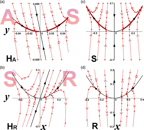
Let the map , G:R ²→R ². Let JG(X*) be the Jacobian matrix of G at the fixed point X*= (x*, y*). Then, the map G may be written in the form of the following difference equation:

where the map [Gtilde] contains all the higher order terms 12. Let us assume that one of the eigenvalues of, say λ₁=1, and the other eigenvalues is . We also assume that JG is the following diagonal matrix:

Now Equation (9) may be written as

The existence of a centre manifold for Equation (11) is guaranteed by the following theorem.

Theorem 2

(Invariant manifold theorem) 3 16. Assume that and . For the eigenvector is E ^c. Let us split the case of into two subcases, and , where E ^u and E ^s are the corresponding eigenvectors. Suppose now that F∈C ². Then there exist a centre manifold W ^c and a stable W ^s (or an unstable manifold, respectively tangent to E ^c and E ^s (or at the fixed point X=0. Moreover, all the manifolds W ^c, W ^s and W ^u are invariant (both positively and negatively invariant).

Now let the centre manifold be given by y=h(x). Throughout this section we consider the case where λ₁=1. Then substituting in Equation (11), yields where the map u(x) is given by

where x* is the first component of the fixed point X*. In order to have semistability on the centre manifold h(x) of the map u(x), one must have, , and (Theorem 1, 6). We demonstrate the semistability by the two following examples for the two cases (i) λ₂<1, and (ii) λ₂>1. Furthermore, we provide two additional examples that show how this semistability may be destroyed if .

Example 1

Semistability with λ₁=1 and λ₂<1:

There is a unique fixed point X*=(0, 0). We write the centre manifold as y=h(x), and substituting in Equation (13) we obtain

that is

or

that is

where we set . Then, we easily conclude that h(x)=x ² by comparing both sides of Equation (17). Now , and, thus, the centre manifold is semistable from the left by Theorem 1.

Example 2

Semistability with λ₁=1 and λ₂>1:

There is a unique fixed point X*=(0, 0). Again, substituting y=h(x) in Equation (18) we obtain

that is

or

that is

where again we set and conclude that h(x)=x ². Now , . Hence, the centre manifold is semistable from the left by Theorem 1.

Example 3

λ₁= 1 and λ₂ \textless 1 without semistability:

There is a unique fixed point X*= (0, 0). We write the centre manifold as y=h(x), and substituting in Equation (23) we obtain

that is

or

where we set . Again we conclude that h(x)=x ². Equation (26) becomes , where g ₁ (0)=0, , , . By a theorem in 9, if and , the fixed point x=0 is unstable under the map g ₁(x). Hence, the centre manifold W ^c is unstable. Therefore, in order to obtain semistability, it is necessary to have .

Example 4

λ₁=1 and λ₂>1 without semistability:

The reader may easily show that the centre manifold W ^c is h(x)=x ², but similar to the previous example, we have , with and , and thus, W ^c is unstable again.

Remark

	(1) In the case of negative eigenvalues λ2<0 we obtain the same dynamics but with oscillations. We omit the discussion of this case.
	(2) In the case of negative eigenvalue , the centre manifold dynamics do not involve semistability as was explained earlier. The centre manifold may be stable or unstable so that the fixed point in the plane is either a repeller (R), a saddle (S), or an attractor (A) (depending on the second eigenvalue).

In Figure 2, we demonstrate the creation of a semistable fixed point associated with λ₁=1 and (a) λ₂>1, (b) λ₂<1, by ‘merging’ through bifurcation the two fixed points of stability R (or A) and S. The yellow-shaded region in each panel shows the degenerated orbits of the discrete flow. In Figure 2(a), the degenerated orbits start near R, passing asymptotically near S, and diverge to infinity. As the R and S fixed points are getting closer to each other (by setting suitably the map's parameters), the yellow regions shrink while the outer dynamics remain basically the same. The first eigenvalue that in our example operates on the horizontal axis, λ₁>1 on the left-hand side graph of the R fixed point, and λ₁<1 on the right-hand side graph of the S fixed point, approaches λ₁=1, where the bifurcation occurs. Similar explanation may be given for Figure 2(b). The degenerated orbits of the discrete flow come from infinity, passing asymptotically near S, and converge to A. The first eigenvalue λ₁<1, on the left-hand side graph of the fixed point A, and λ₁>1, on the right-hand side graph of the fixed point S, approaches λ₁=1 where bifurcation occurs. The second eigenvalue, operating on the vertical axis, retains its dynamics in this bifurcation, that is, (a) λ₂>1 and (b) λ₂<1. Thus, the ‘created’ semistable fixed points have λ₁=1 and (a) λ₂>1 or (b) λ₂<1, denoted by H _R or H _A , respectively.

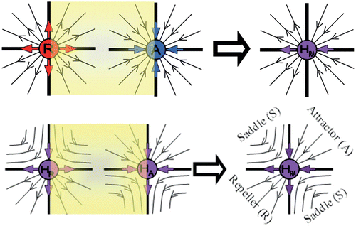
In all the above, we defined and described in detail, planar semistable fixed points that have only one eigenvalue that equals one (λ₁=1). Now we explore the cases when both eigenvalues equal one (λ₁=1, λ₂=1). Though this case will not be thoroughly studied here, we will, however, demonstrate all the possible scenarios of this semistability. One possible combination is the utilization of R and A fixed points, as shown in Figure 3(a). The resulting semistable fixed point has both eigenvalues equal to 1. The vertical axis is a separatrix, dividing the outward discrete flow on the left-hand side with the inward discrete flow on the right-hand side. For this reason, we denote this semistable fixed point as H _RA .

The three semistable fixed points H _R , H _A , and H _RA are created through a new type of bifurcation of the fixed points of regular stability R, A, and S (first-generation semistability). More complicated structures may be obtained through the bifurcation of any two semistable fixed points (second-generation semistability). As an example, we depict the case of the bifurcation of H _R and H _A in Figure 3(b). The result is a fixed point with different dynamical behaviour in each quadrant. In particular, in the first quadrant the created fixed point behaves as an attractor A, while in the third quadrant as a repeller R; in the second and fourth quadrants the fixed point behave as a saddle S. The dynamics of this semistable point is similar to H _RA . The main difference is that when H _RA is created through bifurcation of R and A (first-generation semistability), the saddle behaviour (second and fourth quadrants) degenerates into a separatrix (coinciding with the vertical axis).

Figure 2. Two different types of semistable points H _R and H _A can be seen as ‘merging’ two ordinary fixed points through a bifurcation, that is a repeller (R) + a saddle (S) (upper graphs) (see also Figure 1(b)), and an attractor (A) +a saddle (S) (lower graphs) (see also Figure 1(a)).

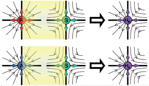
Figure 3. Semistable point H _RA is created through a bifurcation of the ordinary fixed points of stability R and A, or of the first-generation semistability points H _R and H _A . The semistable point H _RA on the top-right figure is a special case of the semistable point H _RA depicted on the lower right figure, where the second and fourth quadrants that behave as a saddle S degenerate to a separatrix (coinciding with the vertical axis) that consists entirely of fixed points.

Remark

In the case of eigenvalues λ₁=1 and , and if both of the centre manifolds exist, then we will have the same dynamics as in the case of λ₁=1 and λ₂<1 (or λ₂>1), but with oscillations, leading again to the semistable fixed points H _A and H _R . This is due to the fact that the centre manifold corresponding to is either stable or unstable and cannot be semistable (Theorem 1).

In the sequel, we will utilize the fixed points R, A, S and H _R , H _A , H _RA to characterize the Allee effect in planar models.

3. General Allee effect

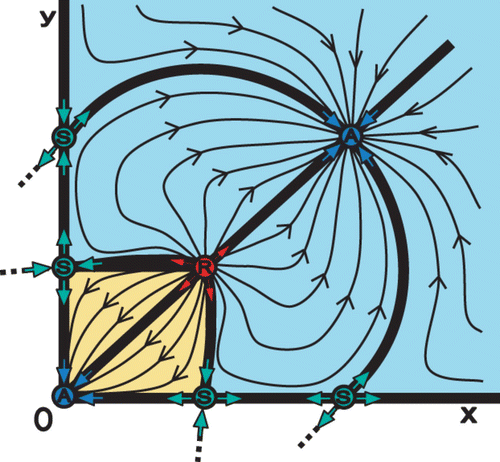
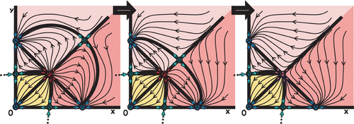
We start our approach by using the planar Λ-Ricker map (5). In Figure 4 we plot the phase space for values of the parameters , , k ₁=k ₂=1.7. There are seven fixed points, with an attractor A at the origin (0, 0), a pair of S and A at each axes, and a pair of R and S in the first quadrant. Furthermore, each species possess the strong Allee effect that is represented by the well-known one-dimensional Allee effect, located between the S fixed point on each axis and the attractor A at the origin. Moreover, we have two new fixed points, a repeller R, called the planar Allee point, and a saddle S, called the planar-carrying capacity. The separatrices are heteroclinic orbits.

Figure 4. The phase space for the planar Λ-Ricker map (5) with parameters Λ₁=Λ₂=2, b ₁=b ₂=c ₁=c ₂=1, k ₁=k ₂=1.7 (symmetric map).

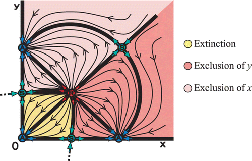
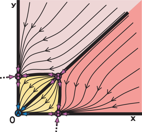
An interesting scenario occurs when two heteroclinic orbits connect two saddle points S on the two axes with an interior repeller point R (Figure 4). The two orbits lie on the stable manifolds of the saddle points on the axes. These two manifolds separate the extinction region (yellow) from the exclusion regions of species x (light red), and y (red). Notice that the boundary of the extinction region consists of the above-mentioned two stable manifolds and the two axes x and y. Therefore, if the initial point (x ₀, y ₀) lies in the extinction region, then both species will go extinct. Now we formalize the above discussion.

Definition The planar extinction region or Allee basin is the basin of attraction of the origin; its boundary in the interior of the first quadrant defines the planar Allee curve. Moreover, a planar Allee point is any positive fixed point that lies on the planar Allee curve.

Remark

	(1) Notice that the Allee curve encloses the extinction region, but not the two axes that correspond to one-dimensional Allee effect and include only the Allee point.
	(2) An Allee point must be either of type R, S, or H, but cannot be of type A; this is self-evident, since then part of the extinction region will be in the basin of attraction of the Allee point A, an absurdity.
	(3) The notions of planar Allee curve and planar Allee point generalize, in a natural way, the Allee point threshold point in the (one-dimensional) dynamics of single species.
	(4) The planar extinction region generalizes the one-dimensional extinction interval of each species that in each axis segment bounded by the origin and the one-dimensional Allee point S.
	(5) The certain arrangement of the four fixed points located on the boundaries of the extinction region (e.g. A–S–R–S in Figure 4) is not random. On the contrary, this certain permutation of fixed points is valuable for having the strong Allee effect and it is called ‘core’ of the Allee effect. In the next section, we will expose all the possible arrangements of fixed points that construct a core.

The planar Allee point R in the above remarks leads to the following definition.

Definition A planar competition model is said to possess the strong Allee effect properly if its phase space exhibits an extinction region and a non-extinction region separated by an Allee curve.

We now resume our investigation of the planar map (8) of two competing species exhibiting contest inter-specific competition. As we mentioned, depending on the parameter values we may have nine fixed points (see Section 1). A diagram of the phase space is given in Figure 5 for a ₁=2.5, a ₂=2.5, b ₁=0.1, b ₂=0.1. We observe the presence of an Allee curve that passes through three planar Allee points (similar to Figure 4). Two of the planar Allee points are the fixed points S that correspond to one-dimensional Allee points (placed on the axes); the third Allee point is the interior fixed point R. In addition, the two one-dimensional-carrying capacities points A are present. The interior saddle point S in Figure 4, that is changed to A in Figure 5, is a planar-carrying capacity point. Moreover, in Figure 5 there are two new interior S fixed points surrounding the mentioned planar-carrying capacity point A. Both the interior saddle points S and the attractor A are characterized by a stable manifold emanating from the R Allee point. Therefore, we give the following definition for the planar-carrying capacity curve and points.

Definition A planar-carrying capacity is a fixed point with one stable manifold emanating from an Allee point. The planar-carrying capacity curve may connect all or a subset of the planar-carrying capacities. The dynamics of the planar-carrying capacities have to be A, S, or H, and not R (since R has no stable manifolds).

The two planar-carrying capacities S (Figure 5) separate the exclusion regions from the coexistence region. It is noteworthy to mention that the four regions of (1) extinction (yellow), (2) exclusion of species y (red), (3) exclusion of species x (light red), and (4) co-existence (light blue) are either the basin of attraction of A fixed points or the stable sets of H fixed points.

Generally speaking, planar maps may exhibit only two of the critical regions of extinction, exclusion, and co-existence. The example in Figure 4 shows a case with extinction and exclusion regions, while for planar maps that do not exhibit strong Allee effect there are only exclusion and coexistence regions. Theoretically, we may be able to observe phase spaces with only extinction and coexistence regions, as shown in Figure 6. This is the phase space of Figure 4, after exchanging the S carrying capacity points to A, and vice versa.

Moreover, Figure 7 demonstrates how the Allee point R merges with the carrying capacity S through a bifurcation, by varying suitably the parameters (while keeping the symmetry of the system). The result of the bifurcation is a semistable fixed point H _R , as defined in Section 2. The core is still present, but is constructed by different permutations of fixed points since R is replaced by H _R .

Notice that in the case of the symmetric planar Λ-Ricker map, the semistable point in the interior appears for . For other selections of the parameters, the two fixed points on each of the axes may be merged through a bifurcation into a semistable point. The bifurcation leads to a semistable fixed point H _A . For the symmetric Λ-Ricker map, this occurs when for the x-axis and for the y-axis. Figure 8 shows a hypothetical case where all three semistable points (two H _A fixed points at each axis and one H _R fixed point in the interior) appear simultaneously.

Finally, we are in a position to give details and explanations of the notion of the ‘core’ of the Allee effect.

Figure 5. The phase space for the planar map of (8) (competition model that exhibits contest inter-specific competition) and a selection of the parameter values a ₁=a ₂=2.5, b ₁=b ₂=0.1 (symmetric map).

Figure 6. A hypothetical phase space with only extinction and coexistence regions.

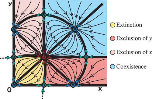
Figure 7. In the symmetric planar Λ-Ricker map, the two interior fixed points of a repeller (R) and a saddle (S) are merged through a bifurcation into one semistable fixed point when k=ln (2). Panels show a gradual decrease of k: (a) k=1.7, (b) k=1 and (c) k=ln (2). The generated semistable point (indicated by H) is of type H _R (Figure 2).

Figure 8. Phase space with three semistable points (indicated by H), two H _A fixed points at each axis and one H _R fixed point in the interior.

4. The core of Allee effect

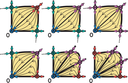
Different arrangements of the surrounding fixed points may lead to different cores of the Allee effect. Figure 9 shows the three possible different cores of the Allee effect, one with three fixed points (A–R–S) and two with three fixed points (A–S–R–S, A–R–S–R).

Figure 9. The three possible arrangements of fixed points that construct a core of the Allee effect.

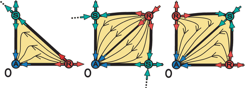
The semistable fixed points H _R , H _A , and H _RA increase the possible permutations of the core. This can be realized in two possible ways. (i) By replacing fixed points of regular stability A, R, S; (ii) Having double role as fixed points. For example, in the upper panels of Figure 10 we observe semistable fixed points H _R and H _A replacing regular fixed points R and S, respectively. However, in the lower panels we observe the double role of H _R (as R and S) and H _A (as A and S).

Figure 10. Semistable fixed points H _R and H _A replace regular fixed points R and S, respectively, as it is shown in upper middle and right panels. The double role of H _R (as R and S) and H _A (as A and S) is shown in the lower panels. (Both H _R and H _A are indicated by H.)

5. Discussion and conclusions

In 4 the authors laid down the consequences of Allee effects for population and community dynamics. We see at least two fruitful avenues for future research on Allee effect. The first avenue is to learn much more about effects of positive density dependence on population dynamics by recognizing and modelling impacts of multiple Allee effects, i.e. in two or more fitness components 4. The second avenue, which is more relevant to this paper, is to investigate the Allee effect for multi-species systems.

In a series of papers, Deredec and Courchamp 7 8 studied the impact of Allee effect on host populations in a host–parasitoid systems. Like most of the literature on population dynamics (e.g. 5), they used differential equations for modelling populations with the Allee effect.

In this paper, we have developed a theoretical foundation for discrete models of populations with the strong Allee effect, described by difference equations. These models describe populations that exhibit a ‘critical size’ below which the population declines on average and goes to extinction, and above which it increases on average. To illustrate our concepts, we investigated two planar models with the Allee effect and showed all the related possible scenarios of phase space diagrams. These are (i) the Λ-Richer competition model, and (ii) a specific model of contest inter-specific competition. These models belong to a class of systems that possess ‘intraspecific’ Allee effect, in which the Allee effect is caused by the intra-specific competition (competition among members of the same species), and not by the inter-specific competition (competition between individuals of different species). This work may be applicable to both intra-specific and inter-specific competition models.

Moreover, we presented a general framework for the notion of strong Allee effect in planar discrete semi-dynamical systems but restricted to the dynamics of equilibria, as shown by the following four paragraphs:

•	A significant idea in the paper is the introduction of the ‘Allee curve’, which is the boundary of the basin of attraction of the origin (0, 0) that separates the extinction region from the rest of the phase space, and thus generalizing the concept of ‘Allee-point’ in one-dimensional dynamics.
•	We described the essential dynamics that characterize the strong Allee effect within the basin of attraction of the origin that is bounded by the Allee curve. This is called the ‘phase space core’ of the Allee effect and consists of only three or four fixed points. The regular type of fixed points (repeller, saddle, and attractor) combine three different types of cores. However, semistable fixed points increase the variety of ‘phase space cores’.
•	We introduced and thoroughly characterized the notion of semistability in planar discrete semi-dynamical systems, and showed its crucial role in the Allee effect dynamics. Two categories of semistable fixed points are defined, and their phase spaces are studied in accordance with the regular type of fixed points.

In a future work, we will investigate thoroughly the dynamics of both scrambled competition models with the strong Allee effect and contest competition models with the strong Allee effect. Moreover, we will study the cases of periodic orbits in the presence of the strong Allee effect.

Notes

This is a paper based on an invited talk given at the 3rd International Conference on Math Modeling & Analysis, San Antonio, USA, October 2011.

References

- Allee , W. C. , Emerson , A. E. , Park , O. , Park , T. and Schmidt , K. P. 1949 . “ Principles of Animal Ecology ” . Philadelphia : WB Saunders .
- Allee , W. C. and Rosenthal , G. M. 1949 . Group survival value for Philodina roseola, a rotifer . Ecology , 30 : 395 – 397 .
- Carr , J. 1981 . “ Applications of Centre manifold theory ” . New York : Springer-Verlag .
- Courchamp , F. , Berec , L. and Gascoigne , J. 2008 . “ Allee Effects in Ecology and Conservation ” . Oxford : Oxford University Press .
- Cushing , J. M. and Hudson , J. T. Evolutionary dynamics and strong Allee effects . J. Biol. Dyn. , to appear
- Dannan , F. M. , Elaydi , S. and Ponomarenko , V. 2003 . Stability of hyperbolic and non-hyperbolic fixed points of one-dimensional maps . J. Difference Equ. Appl. , 9 : 449 – 457 .
- Deredec , A. and Courchamp , F. 2003 . Extinction thresholds in host–parasite dynamics . Ann. Zool. Fenn. , 40 : 115 – 130 .
- Deredec , A. and Courchamp , F. 2006 . Combined impacts of Allee effects and parasitism . Oikos , 112 : 667 – 679 .
- Elaydi , S. 2008 . “ Discrete Chaos with Applications in Engineering and Science ” . Boca Raton , FL : Chapman & Hall/CRC .
- Elaydi , S. and Kang , Y. “ Allee effects in two species interactions ” . preprint
- Elaydi , S. and Sacker , R. 2010 . Population model with Allee effect: A new model . J. Biol. Dyn. , 4 : 397 – 408 .
- Guzowska , M. , Luis , R. and Elaydi , S. 2011 . Bifurcation and invariant manifolds of the logistic competition model . J. Difference Equ. Appl. , : 1851 – 1872 .
- Jang , S. R.-J. 2006 . Allee effects in a discrete-time host–parasitoid model . J. Differential Equation Appl. , 12 : 165 – 181 .
- Kulenović , M. R.S. and Yakubu , A.-A. 2004 . Compensatory versus overcompensatory dynamics in density-dependent Leslie models . J. Difference Equ. Appl. , 10 : 1251 – 1265 .
- Lidicker , W. Z. 2010 . The Allee effect: Its history and future importance . Open Ecol. J. , 3 : 71 – 82 .
- Luis , R. , Elaydi , S. and Oliveira , H. 2010 . Non-autonomous periodic systems with Allee effects . J. Difference Equ. Appl. , : 1179 – 1196 .
- Marsden , J. E. and McCraken , M. 1976 . “ The Hopf Bifurcation and its Applications ” . New York : Springer-Verlag .
- Mohamad , R. , Monge , J.-P. and Goubault , M. 2011 . Agonistic interactions and their implications for parasitoid species coexistence . Behav. Ecol. , 22 : 1114 – 1122 .
- Schreiber , S. J. 2003 . Allee effects, extinctions, and chaotic transients in simple population models . Theor. Popul. Biol. , 64 : 201 – 209 .
- Wang , G. , Liang , X.-G. and Wang , F.-Z. 1999 . The competitive dynamics of populations subject to an Allee effect . Ecol. Model. , 124 : 183 – 192 .