The role of adaptations in two-strain competition for sylvatic Trypanosoma cruzi transmission

Abstract

This study presents a continuous-time model for the sylvatic transmission dynamics of two strains of Trypanosoma cruzi enzootic in North America, in order to study the role that adaptations of each strain to distinct modes of transmission (classical stercorarian transmission on the one hand, and vertical and oral transmission on the other) may play in the competition between the two strains. A deterministic model incorporating contact process saturation predicts competitive exclusion, and reproductive numbers for the infection provide a framework for evaluating the competition in terms of adaptive trade-off between distinct transmission modes. Results highlight the importance of oral transmission in mediating the competition between horizontal (stercorarian) and vertical transmission; its presence as a competing contact process advantages vertical transmission even without adaptation to oral transmission, but such adaptation appears necessary to explain the persistence of (vertically-adapted) T. cruzi IV in raccoons and woodrats in the southeastern United States.

Keywords:

• Trypanosoma cruzi
• horizontal transmission
• vertical transmission
• trade-off
• cross-immunity

MSC 2010 :

• 92D15
• 92D30
• 92D40

View correction statement:

Erratum

1. Introduction

†Evolutionary epidemiology describes the adaptation of pathogens to selection pressure in host populations. The protozoan parasite Trypanosoma cruzi offers an opportunity to extend this field in two ways: by considering vector-transmitted disease, where host–vector cycles present a more complex landscape for pathogen evolution, and by considering interstrain competition as a selective force driving specialization towards distinct transmission modes. This pathogen, native to the Americas, is enzootic in host–vector cycles from the central USA to the southern cone, involving hundreds of mammalian host species and dozens of triatomine vector species. Although T. cruzi is best known as the etiological agent of Chagas’ disease, affecting millions of people throughout Latin America, it is the sylvatic cycles which maintain the parasite, with vectors infected in the wild continually moving to human habitations in search of new bloodmeal sources. In the USA, where Chagas’ disease is little-known, recent concerns in this regard have focused on the risk of transmission by transfusion or organ transplants from individuals (including immigrants) infected in Latin America. As a result, the sylvatic cycles in the USA have been less studied despite the often high (over 50%) prevalence of infection observed in some sylvatic US hosts. Only recently have studies begun to examine the characteristics particular to the sylvatic infection cycles that keep T. cruzi in zoonosis in the USA (some recent relevant summaries include 12 19 23 41).

In the southeastern United States (SE US), in a region extending from eastern Texas to the Atlantic coast, the primary T. cruzi hosts are raccoons (Procyon lotor) and Virginia opossums (Didelphis virginiana). The main vector species associated with these hosts is Triatoma sanguisuga (other members of the Triatoma lecticularia complex which includes T. sanguisuga have also been observed). To the west of this region, in parts of Texas and northern Mexico dominated by desert scrub, Triatoma gerstaeckeri is the dominant species, associated in sylvatic settings almost exclusively with the southern plains woodrat (Neotoma micropus). Strains of T. cruzi have been classified by phylogenetic lineage as belonging to one of six types, I–VI (formerly I and IIa–e); while all six types cocirculate in South America, only types I and IV (formerly IIa) have been identified in the USA 39. Type I, which is associated with Chagas’ disease and human infections, is the only type found in Virginia opossums, as they have been found immune to type IV 41, consistent with the association of South American opossums with type I infections there 50. Other sylvatic US hosts, including raccoons (as well as skunks, foxes, and armadillos), are associated instead with T. cruzi IV 17 39. Most recently, both strains have been found in Texas woodrats 5.

The traditional means of infection with T. cruzi involves the vector feeding on a host. Vectors become infected via a bloodmeal on an infected host, following which the parasite reproduces in the vector's gut. Hosts become infected when the parasite comes into contact with their mucous membranes or with a lesion in the skin; typically the vector defecates near the feeding site shortly after feeding, and the host scratches the bite area, inadvertently rubbing the parasite into the wound. This is referred to as stercorarian transmission. Vertical (congenital) transmission, which has been observed in humans as well as laboratory rats 28 43, may also be significant among other placental hosts (but not in marsupials such as opossums). Furthermore, it has been suggested that oral transmission of T. cruzi via host consumption of infected vectors (raccoons and opossums are both opportunistic feeders whose diets include insects) may be the dominant infection pathway in some cycles, more likely among raccoons than among opossums 32 37 40 49. Oral transmission has also been documented in laboratory mice as well as in humans 4 7 and other primates 35. Oral transmission is a risky adaptation in evolutionary terms since the consumed vector can infect at most one host this way, as opposed to potentially many via stercorarian transmission, but as shown in 24 it can, under some conditions, maintain sylvatic cycles alone. Indeed, it may not be any riskier than stercorarian transmission, which by its nature is less efficient than the more classical vector-borne transmission seen in mosquito-transmitted diseases, where vector feeding transmits the parasite directly into the host from the vector's salivary glands.

In the SE US, the vectors T. sanguisuga and T. gerstaeckeri have long been observed to be inefficient vectors 33 because of their cautious feeding behaviour – they avoid climbing completely onto the host – and the long mean time between feeding and defecation. As a result, other avenues of transmission may be more important to maintaining the sylvatic cycles found in the SE US. In particular, the vectors’ inefficiency at stercorarian transmission may make oral and vertical transmission successful competition strategies when T. cruzi is under strong selection pressure to increase its host infection rate, either by improving its stercorarian transmission rate or by adapting to other transmission modes. Each of these modes involves a different mechanism for which pathogen strains may be more or less adapted. Each transmission cycle (host–vector association) has unique characteristics (vector–host density ratio, host predation rate on vectors, etc.) which can shape adaptation by advantaging one transmission mode over others.

Infection with a given strain of T. cruzi has been observed 26 31 to confer immunity against infection by other strains. This cross-immunity highlights a competition between strains for access to hosts and vectors, and one hypothesis is that this competition has driven adaptations in the strains to specific modes of transmission in order to persist. In particular, T. cruzi IV is often described as being less virulent than type I 30 38 44, but appears to be better adapted to vertical transmission (by a factor of 2 in one study 17), and may also be better adapted to oral transmission, to both of which raccoons – the target host for type IV in the SE US since opossums are immune to it – are more vulnerable than opossums, as noted above. (Neither of these modes has yet been studied in woodrats.) Theory developed for directly transmitted pathogens suggests that a trade-off occurs between vertical and horizontal (classical) transmissibility 27 42. This trade-off postulates a correlation between virulence and transmission, holding that more virulent – and hence more transmissible by classical means – strains should be favoured when hosts are numerous, and less virulent strains – which, being less harmful to hosts, may make vertical transmission more successful – when hosts are scarce 46. Such theory is not well-established for vector-transmitted diseases, where new factors come into play. For example, the relative efficiency of different transmission modes may depend on the vector–host density ratio (when it is low, hosts are plentiful relative to vectors, so may not be bitten as often – does this scenario then favour alternative transmission modes?). In addition, in the case of T. cruzi in the SE US, pathogen-related mortality is not customarily observed in the primary hosts, so any notion of virulence associated with horizontal (here, stercorarian) transmission to hosts must be clarified. The present study focuses on the trade-off between stercorarian transmission and vertical (and perhaps oral) transmission hypothesized to occur in T. cruzi strains competing in sylvatic cycles in the SE US.

Although evidence of such evolutionary adaptations remains circumstantial and indirect at present, the competition between strains can be studied theoretically using mathematical models. Most theoretical studies of T. cruzi transmission have heretofore been limited to domestic transmission involving humans, including by transfusion 36 48, but modelling has been used to study many other vector-borne diseases, including vertical transmission in dengue vectors 14. Variable adaptation to vertical transmission has been studied in infections transmitted purely horizontally 1 9 15, including Dhirasakdanon and Thieme's 9 finding of persistence in vertically transmitted parasite strains that provide cross-immunity against infection by more virulent strains transmitted purely horizontally, a situation not unlike the competition hypothesized between T. cruzi I and IV here. The contact process(es) that drive the transmission of pathogens between two distinct populations, however, saturate in one or the other population, as a function of the ratio of the two densities. Recently, Kribs–Zaleta 21 23 24 developed models for sylvatic T. cruzi transmission which incorporate stercorarian, oral and vertical transmission to hosts, finding that for cycles involving raccoons and opossums the feeding processes of both hosts and vectors are likely saturated in vectors, and hence primarily dependent on host population density, and also that oral transmission is likely the dominant means of infection for raccoons in the SE US, even if raccoon predation on vectors is rare, thanks in part to a boost by vertical transmission. For woodrats, meanwhile, estimates 23 suggest that the two processes are saturated in different densities, leading to potentially different selection pressures and different interstrain competition outcomes.

The present study builds on this work by extending the models to examine the competition between T. cruzi I and IV in cycles involving a placental host such as raccoons or woodrats, and the vector T. sanguisuga or T. gerstaeckeri (respectively), in order to describe the role played by possible evolutionary adaptations in determining the outcome of this competition. The next section develops a model to describe the underlying dynamics and establishes a framework for evaluating adaptation's influence on the competition, through a trade-off between transmission modes. Analysis of the resulting dynamics focuses on reproductive numbers for the infection, which permit evaluation of the role of adaptive trade-offs between transmission modes on the interstrain competition. We consider raccoon-T. sanguisuga and woodrat-T. gerstaeckeri cycles separately since disparities in the vector–host ratio, host (predator) functional response, and other characteristics may shape adaptation differently.

2. Model formulation

2.1. Underlying dynamics

To describe the competition between T. cruzi I and IV, we extend the host–vector infection model of 24 to a two-strain model, summarizing first the underlying assumptions. For simplicity in modelling vertical transmission, we consider only female hosts, and assume that a proportion p _j (j=1, 2) of hosts infected with strain i give birth to infected young. There is no vertical transmission in vectors since parasites reside only in the gut of infected vectors. Rates for both types of feeding contacts – vector bloodmeals, which lead to vector infections of type j (j=1, 2) at rate c _vj and to stercorarian infection of hosts with strain j at rate c _hj (both in units of 1/time), and host predation (effort, in units of vectors/host/time) E _h on vectors – are assumed to depend on the vector–host population density ratio 2. A proportion ρ _j of hosts that consume a vector infected with strain j become infected with that strain. We also assume simple demographics for both host and vector, e.g. logistic reproduction and linear per capita mortality.

Since sharp saturation in contact rates (such as piecewise linear, corresponding to Holling type I) has been shown to exhibit a wider variety of behaviours than smooth saturation (such as Holling type II) 20–22, we initially consider the three contact rates mentioned above to follow such (piecewise linear) sharp saturation, defining:

as in Equation (2) of 24, with maximum values , (j=1, 2) and H, respectively, and respective saturation thresholds Q _v (for vector feeding) and Q _h (for host predation). Thus, the host-related rates c _hj and E _h saturate for high vector–host ratios, while the vector-related infection rate c _vj saturates for low vector–host ratios.

Variables, notation, and parameters are summarized in Tables 1 and 2, with baseline parameter estimates either taken from 23 or developed in Appendix 1. Here the total vector density is , and similarly for N _h, while the total vector birth rate is given by the function b _v, say , and analogously for the host birth rate b _h. The resulting dynamics can be summarized by the flowchart in Figure 1 and by the following system of ordinary differential equations:

Figure 1. Flow chart illustrating model (2). All rates given are per capita except birth rates. For space constraints, the notation C _j =[c _hj (Q)+ρ _j E _h(Q)]I _vj /N _v (j=1, 2) is used.

Table 1. Variables and notation for sylvatic T. cruzi transmission model.

Var.	Meaning	Units
S h(t)	Density of uninfected hosts	hosts/area
I h1(t)	Density of hosts infected with T. cruzi I	hosts/area
I h2(t)	Density of hosts infected with T. cruzi IV	hosts/area
S v(t)	Density of uninfected vectors	vectors/area
I v1(t)	Density of vectors infected with T. cruzi I	vectors/area
I v2(t)	Density of vectors infected with T. cruzi IV	vectors/area
Q	Vector–host population density ratio ()	vectors/host
	Strain j stercorarian infection rate	1/time
	Strain j vector infection rate	1/time
	Per-host predation rate	vectors/host/time

Table 2. Parameter definitions and estimates (from 23 and Appendix 1) for sylvatic T. cruzi cycles involving raccoons and T. sanguisuga (R/S), woodrats and T. gerstaeckeri (W/G).

Parm.	Definition	Units	R/S	W/G
r h	Maximum growth rate for hosts	per year	0.90	1.8
r v	Maximum growth rate for vectors	per year	33	100
μh	Natural mortality rate of hosts	per year	0.40	1
μv	Natural mortality rate of vectors	per year	0.271	0.562
N h*	(Equilibrium) host population density	hosts/acre	0.080	9.3
K h	Carrying capacity for hosts	hosts/acre	0.14	21
N v*	(Equilibrium) vector population density	vectors/acre	128^a	128
K v	Carrying capacity for vectors	vectors/acre	129^a	129
Q h	Threshold vector–host density ratio for predation	vectors/host	10	10
Q v	Threshold vector–host density ratio for bloodmeals	vectors/host	100	100
	Maximum stercorarian infection rate	per year	0.525	13.5
	vector infection rate	per year	9.67	1.59
p max	Maximum vertical transmission proportion	dimensionless	0.15	0.375
H	(Maximum) per-host predation rate	vectors/host/yr	1	1
ρmax	Maximum proportion of hosts infected after consuming an infected vector	hosts per vector	1	1
ρ	Estimated proportion of hosts infected after consuming an infected vector	hosts per vector	0.177	0.177
^aVector density estimates for this cycle were taken from that for the other cycle, which is the only published vector density estimate. See 23 for discussion.

The estimates derived in 23 imply that in practice for the raccoon-T. sanguisuga transmission cycle, so that both types of host–vector contact processes are saturated in vectors and thus driven by host density, while for the woodrat-T. gerstaeckeri transmission cycle . We therefore take the corresponding terms from Equation (1), making

for the raccoon-T. sanguisuga transmission cycle, while

for the woodrat-T. gerstaeckeri transmission cycle. We consider these two cycles separately in the numerical work that follows, in order to see how the changes in saturation status affect T. cruzi interstrain competition for hosts.

2.2. Adaptive trade-off

The trade-off between adaptations to distinct transmission modes manifests in the dynamical model of Section 2.1 through the host infection parameters (stercorarian), p _j (vertical) and ρ _j (oral) for each strain. In order to explore the effects of this trade-off, we rewrite these parameters to make the degree of specialization explicit. In particular, we define variables x, y, and z to be the respective degrees of specialization towards stercorarian, vertical, or oral transmission, with a value of 1 representing full adaptation towards the given transmission mode and a value of 0 representing adaptation away from it (i.e. a complete inability to transmit via that mode). Then for a given strain j, we can write , , and , with . The nature of relevant evolutionary trade-offs can now be described as relationships among x, y, and z.

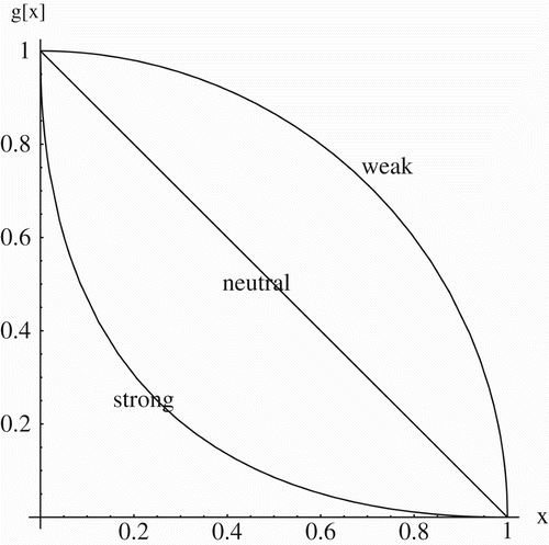
In this study, we assume that a trade-off exists between stercorarian and vertical transmission, so that x=1 implies y=0, and y=1 implies x=0. The trade-off is described by the relation y=g(x), where defines the nature of the trade-off. Trade-off is typically described qualitatively as strong, neutral, or weak, depending on the relative gains and losses at each degree of specialization (see Figure 2). Strong trade-offs mean that specialists (x=0 or x=1) lose more in their specialty than they gain in the other type of transmissibility as they move away from the extremes, creating a curve that is concave down. Under weak trade-offs, specialists gain more in the other type of specialty than they lose in their own as they move away from either extreme, creating a curve that is concave up. In a neutral trade-off, gains or losses in either specialty are exactly offset by corresponding losses or gains in the other specialty. To describe these trade-offs mathematically, we use the symmetric curve 25, where α is a dimensionless parameter measuring the strength of the trade-off. In this study, we shall use α values of ½, 1, and 2 to describe weak, neutral, and strong trade-offs, respectively.

Figure 2. Weak, neutral, and strong trade-offs between two specialties as described by the symmetric function y=g(x)=(1−x ^1/α)^α, with α=½, 1, and 2, respectively.

Since there is not yet any data on whether oral transmissibility is aligned with vertical transmissibility, we shall consider both the case in which oral transmissibility is independent of the stercorarian-vertical adaptation (i.e. z _j is fixed), and the case in which oral transmissibility is aligned with vertical transmissibility (i.e. z _j =y _j ). Finally, in studying trade-off, we assume that with just a single mode of vector infection, and parasites in a different life stage within vectors than within hosts, vector infection rates are unaffected by the trade-off, i.e. .

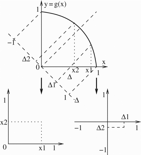
Adaptation along the trade-off curve y=g(x) is typically tracked using x as an index variable, with the spectrum of possible strains varying from x=0 to x=1. However (as observed in 25), for extreme values of the trade-off strength α ( or ) half of the curve (beginning at the midpoint, where x=y) becomes nearly vertical, making it difficult if not (in the limiting cases) impossible to distinguish among these adaptive outcomes using x as an index variable, since their x-coordinates are compressed toward either 0 or 1. That is, for extremely weak trade-offs (), half of the spectrum for which x>y is compressed toward x=1; meanwhile, for extremely strong trade-offs () half of the spectrum for which x<y is compressed toward x=0. In either case x becomes unsuitable as an index variable. It may, therefore, be more helpful to use instead the variable Δ=x−y as an index of a strain's location along the trade-off curve; as x goes from 0 to 1 (and y from 1 to 0), Δ goes from −1 to 1, with the midpoint at 0. This avoids the compression issues at the endpoints. We then evaluate the competition on the subset of the plane. Figure 3 illustrates how any pair of points on the curve y=g(x) corresponds to a unique point in the plane as well as a unique point in the (x ₁, x ₂) plane. This framework shift from x to Δ maintains the notion of the arclength as the genetic distance and hence the primary measure of adaptation. By assumption strain 1 (T. cruzi I) will be taken as further adapted toward stercorarian transmission than strain 2 (T. cruzi IIa/IV), so that x ₁>x ₂, and .

Figure 3. Competition between two strains with adaptation coordinates (x ₁, y ₁) and (x ₂, y ₂) can be studied through pairwise invasibility plots using either x ₁ and x ₂ or Δ₁ and Δ₂, where Δ=x−y. Here x ₁>x ₂.

From adaptive dynamics 10, a pairwise invasibility plot is a useful graphical representation of competition between two variants of an organism, in which the outcome is given for each ordered pair of the two variants’ values of the characteristic which distinguishes them. These plots will be used in the next section after analysis of the infection dynamics provides a fitness measure by which to determine a competition's outcome.

3. Analysis

3.1. Model dynamics

The behaviour of model (2) can be described by studying first the overall host and vector density dynamics, and then simplifying the model to focus on the infection dynamics, where reproductive numbers determine the outcome of the interstrain competition. If we write equations for the total host and vector densities, summing the respective trios of equations in (2), we find that

For most forms of birth rate function , including constant and logistic, Equation (5) has a single globally stable equilibrium N _h* (for instance, if , then ); thus as regardless of initial condition. This leads us to consider Equation (6) for N _v with . As in the simpler models studied in 21 24, the vector density dynamics thus decouple from the infection dynamics, and can be studied separately. As detailed in 21 22, the dynamics of N _v(t) depend on two dimensionless quantities, rescaled versions of the maximum predation rate HN _h* and the saturation threshold , and may exhibit one of four behaviours: (i) the vectors go extinct; (ii) the vectors persist at a unique equilibrium level; (iii) an Allee effect occurs, with extinction and persistence both possibilities depending on initial density; and (iv) the vectors persist at one of two different survival equilibrium densities (each of which then generates a different value for the basic T. cruzi reproductive number R ₀). This last behaviour (positive bistability) occurs for all predator functional responses E _h which saturate more sharply than Holling type II saturation 22; all other behaviours also occur even for smooth saturation in E _h. Vector extinction requires .

In practice, however, high predation on vectors by any T. cruzi host has not been documented, let alone vector extinction as a result. We will, therefore, assume henceforth that vector population dynamics have reached a stable equilibrium level , and by a theorem of Thieme 45 pass to the limiting system of (2) in which , . We can thus eliminate S _h by defining it as , and similarly for S _v. (To simplify notation, we henceforth write N _h, N _v.)

is also fixed in this case, so that

are all constants with respect to time (regardless of whether Q* is greater or less than Q _h and Q _v). The resulting model can thus be further simplified by introducing the following notation: , (j=1, 2), (all with units 1/time). The infection dynamics can thus be studied via the system1

which can be shown to exhibit competitive exclusion, similar to other previously studied models for competing pathogen strains with cross-immunity 3 16. Examination of the steady-state conditions shows system (7) to have three equilibria: the disease-free equilibrium E ₀(0, 0, 0, 0), the equilibrium in which only strain 1 is endemic , and the equilibrium in which only strain 2 is endemic, , where the equilibrium prevalence levels are given by

(No coexistence endemic equilibrium exists except in the trivial case where all parameters are equal.)

In order to describe existence and stability conditions for these equilibria, we must define the basic reproductive numbers R ₁ and R ₂ for strains 1 and 2, respectively, and the invasion reproductive numbers (IRNs) [Rtilde] ₁ and [Rtilde] ₂ for the respective strains. The basic reproductive number for a given strain, a familiar and key quantity in mathematical epidemiology, gives the mean number of secondary infections produced by a single infected individual (host or vector) introduced into a completely naive population. The invasion reproductive number (IRN) gives instead the mean number of secondary infections of the given strain produced by a single infected individual introduced into a population in which the other strain is already endemic 8 34 51. In a cross-immunity context, therefore, . Both reproductive numbers can be calculated using next-generation operator approaches 11 47 (for the IRN, only the invading strain is considered to be an infection, and the endemic equilibrium for the resident strain is used in place of the disease-free equilibrium); the results are as follows:

The overall T. cruzi basic reproductive number is ; some strain of T. cruzi remains enzootic in the given host–vector transmission cycle if R ₀>1. If only one of R ₁ and R ₂ is greater than 1, then the corresponding strain is the one which remains endemic. If both exceed 1, then in theory coexistence could occur if in addition [Rtilde] ₁>1 and [Rtilde] ₂>1. However, some algebra shows that

so it is impossible for both IRNs to exceed 1 simultaneously, which implies competitive exclusion. We can also observe that in these expressions, the vertical transmission terms are separate from the horizontal (other) transmission terms, the latter of which are grouped together as (j=1, 2).

The proofs defining these reproductive numbers in terms of next-generation operators establish local asymptotic stability of the three equilibria: E ₀ alone if R ₀≤1, E ₁ alone if R ₀>1 and [Rtilde] ₁>1, and E ₂ alone if R ₀>1 and [Rtilde] ₂>1 (thus partitioning the entire parameter space into three regions)2. This local stability can be extended to global stability in some cases, as illustrated by the following result, the proof of which (given in Appendix 2) uses a standard application of Lyapunov functions.

If R ₀≤1, the disease-free state E ₀ of system (7) is globally asymptotically stable (GAS). The strain 1 endemic state E ₁ is GAS under any of the following three sets of conditions:

where μ˜_hj =(1−p _j )μ_h, R _j+=β˜_hj β˜_vj /μ˜_hj μ˜_v, and f _j (x)=x/(x+μ˜_hj ) (j=1, 2). Likewise, the strain 2 endemic state E ₂ is GAS under any of the following three sets of conditions:

A note regarding the quantities R _j+ defined above: it is straightforward to prove that , and . The first of these facts implies that (k≠j), reflecting the increased difficulty of invasion when another strain is present. In these terms, we can also write .

3.2. Trade-off and competition

The deterministic model (2) can, therefore, be used to predict the outcome of interstrain T. cruzi competition by identifying which (if either) of the two strains’ IRNs exceeds 1. As observed in Equation (8), the question of which strain's IRN exceeds 1 is mathematically equivalent to which strain [j] has the greater value of the expression . We can rewrite this expression as a function of the degrees of adaptation to stercorarian transmission x and vertical transmission y: without adaptation to/from oral transmission, it is , where

is the relative importance of oral transmission over stercorarian at their maxima, and b=p _max. Similarly, with adaptation to oral transmission aligned with that to vertical, . In both cases, ℋ is an increasing function of both x and y on the unit square. As noted in Section 2.2, since x and y are assumed constrained by the trade-off relation y=g(x), this fitness measure can be written as a function h of a single variable Δ=x−y representing the location along the trade-off curve. Whichever strain has a higher value of then wins the competition. Note that the forward diagonal automatically serves as one boundary where both strains have the same value of h.

Since the h-values of the two endpoints of the spectrum are independent of the trade-off strength α, we consider separately the two cases h(−1)<h (1) and h(−1)>h (1). We first note that ; then, without adaptation to/from oral transmission (AOT), h (1)=k(a+1), while with AOT, h (1)=k. Thus the case h(−1)<h (1) simplifies to (a+1)b<1 without AOT and a+b<1 with AOT.

The pairwise invasibility plots in Figure 4 depict outcomes of the competition (a) without, and (b) with, AOT in the plane. For a neutral trade-off (α=1) the competition is independent of the magnitude of the difference in Δ and is instead entirely determined by the relative fitness of the two extremes – whichever strain is closer to the ‘fitter’ extreme wins. However, as the trade-off becomes stronger or weaker, the other strain gains an increasing area (in the triangle ) in which it wins, until for extreme values of α ( and ), the areas are almost equal. Classical trade-off studies suggest that weak trade-offs favour generalists (i.e. h has a maximum in the interior of [−1, 1]), so for whichever strain is more like the optimal generalist (as measured by h) than the other is, wins. Strong trade-offs, meanwhile, favour specialists (i.e. h’s maximum is at one of the endpoints), so the winning strain must be less like (in terms of h) the generalist which minimizes h than the other is; this can occur by being closer to the winning specialist, but it can also occur by being closer to the losing specialist (a local maximum of h) than the other strain is to the winning specialist.

Figure 4. Competition outcomes (a) without, and (b) with, AOT in terms of the Δ₁−Δ₂ plane, with ℋ(0, 1)<ℋ(1, 0) in the left column and ℋ(0, 1)>ℋ(1, 0) in the right column, as the strength α of the trade-off varies from weak (top) to strong (bottom). Strain 1 wins in lighter shaded areas, strain 2 in darker ones.

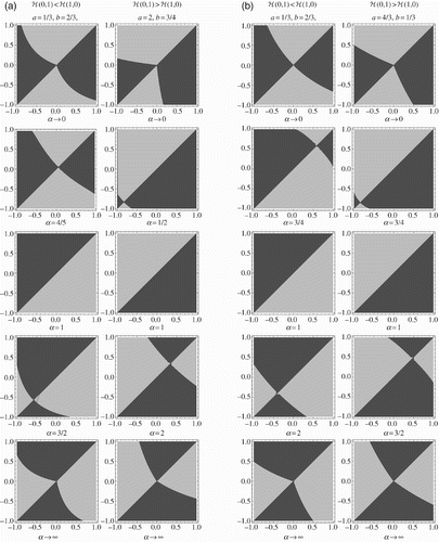
We note that a comparison using x instead of Δ would compress 3/4 of the diagrams representing extreme values of α down into lines with no area; for only the lower left quarter of the diagram would remain, and for only the upper right quarter of the diagram would remain. In both cases (cf. the eight relevant diagrams in Figure 4), the results would suggest that whichever strain has the greater x value (i.e. is more adapted to stercorarian transmission) than the other would win, a result clearly at odds with the more symmetric picture provided using Δ.

It can also be observed that the impact of AOT is quantitative rather than qualitative: if strain 2 is better adapted to both vertical and oral transmission than strain 1, then the region in parameter space in which it wins the competition is larger, but still generally the same shape.

Given the dearth of data from which to estimate several model parameters, one can also consider the effects of variation in parameters such as the maximum predation rate H and the [equilibrium] vector–host ratio Q. Both of these parameters affect the competition through the quantity a:H in a straightforward linear way, Q in a more limited way. Since a involves two saturation processes dependent on Q with different saturation thresholds, as Q rises the process with the lower threshold is advantaged. Estimates suggest here that , making a an increasing function of Q for and independent of Q when both processes are saturated . Thus increasing either parameter makes oral transmission more significant relative to stercorarian transmission, which advantages strain 2 even when both strains are equally orally transmissible.

The baseline parameter estimates developed in Appendix 1, which assume the general vector contact rate of raccoons and opossums to be the same (since they have similar size, eating, moving and sleeping habits) and which assume 10% strain 2 vertical transmission , yield , x ₁=0.755, x ₂=0.431, , , with a=1.90 and b=0.15 for the raccoon-T. sanguisuga cycle, making but a+b=2.05>1. Since α is so close to 1 (i.e. the trade-off is relatively neutral), the competition is determined by the relative fitness of the two evolutionary extremes for most values of x or Δ, including those estimated above. With (a+1)b<1 but a+b>1, strain 2 only wins the competition if it is adapted to oral as well as vertical transmission, although (since here a+b>2) the degree of adaptation need not be as strong as that to vertical transmission.

If we assume that vertical transmission is equally likely in woodrats and raccoons, with p _2w =0.1, then for the woodrat-T. gerstaeckeri cycle a=0.533, making and a+b=0.689<1, i.e. strain 1 should win regardless of AOT. The primary factor contributing to the difference from the raccoon cycle is not the difference in the vector–host ratio Q but the difference in lifespan : a woodrat population is renewed (existing members die and new ones are born) 2.5 times as fast as raccoons, so in order to account for the observed prevalence, any infected woodrats ‘replaced’ by uninfected ones must be infected faster than raccoons. These results (for both cycles) hold for a relatively wide range of values of p (0–0.3) and ρ (0–0.4); higher values (roughly p≥0.5 and ρ≥0.6) are inconsistent with observed prevalence since they would predict higher prevalence even without any stercorarian transmission whatsoever.)

However, if we suppose that rats are more like the lab mice in 18 than like raccoons, strain 2 can win in the woodrat cycle as well. For the given values, if we assume that (hence as in Table 2), then strain 2 wins if adapted to oral transmission, and for higher values of p _2W (e.g. 0.4) strain 2 wins even without AOT. The observation of both strains of T. cruzi in woodrat populations can be understood in terms of this model by taking vertical transmission to occur at a higher proportion than in raccoons, at a level that places the two strains’ fitnesses at roughly equal levels, under which scenario local stochasticity can allow either to dominate.

4. Discussion

The dynamical system used in this study to describe sylvatic T. cruzi transmission dynamics provides a framework for evaluating the competition between the two parasite strains native to the USA through fitness measures derived from the infection's reproductive numbers. The fitness measure used here highlights the interplay among transmission avenues to the host – classical stercorarian transmission, vertical (congenital) transmission, and oral transmission via predation – in determining the outcome of this competition. Although adaptive trade-offs involving virulence and alternative transmission modes (in particular, horizontal versus vertical) are well-studied in the context of directly transmitted infections, this may be the first study of such a trade-off in the context of a vector-borne parasite, and the role of oral transmission as a third mode in mediating adaptation between the other two is especially significant. The outcome of this competition takes on special importance since the strain (T. cruzi I) more adapted to stercorarian transmission is associated with Chagas’ disease in humans, and cross-immunity, which prevents co-infection, implies that if the other strain (T. cruzi IV) can entrench itself in a sylvatic host population via improved vertical transmission, it may constitute a barrier against invasion by the Chagasic strain.

Estimates of infection-related rates and each strain's degree of adaptation (based on comparison of type I infection rates in opossums and type IV infection rates in raccoons in the same region) suggest that for very modest vertical and oral transmission rates, strain IV must adapt to oral as well as vertical transmission in order to win the competition in raccoons (as observed). Under the same assumptions, strain I wins the competition in woodrats, but higher vertical or oral transmission rates (still lower than what has been observed in mice in laboratory conditions) allow strain IV to win. Field observations find both strains present in woodrat populations, which suggests that slightly higher vertical (or oral) transmission rates in woodrats place the competing strains on almost equal ground, where local stochastic effects and limited communication between neighbouring woodrat populations allow each parasite strain to make inroads.

Analysis also shows more generally how oral transmission as a second contact process saturating in the vector–host ratio (and sooner than stercorarian transmission does) acts as an important mediator in the competition (in favour of adaptation to vertical transmission), even when both strains are equally orally transmissible. That is, adaptation to oral transmission (aligned with that to vertical transmission) is not as important to persistence of a primarily vertically transmitted strain as is the mere presence of oral transmission as a competing contact process with classical stercorarian transmission.

Further study of this competition using stochastic and/or multi-host models is warranted by reports of prevalence of T. cruzi I – at trace levels in raccoons 39 and more widespread among woodrats 5 – in transmission cycles where T. cruzi IV is established as enzootic. Although the deterministic model developed in this study predicts competitive exclusion, stochastic models can show how fluctuations in transient dynamics (which may last many years) can slow or even reverse its outcome on a local scale, allowing a strain to persist (and even displace another) when it would be normally expected to die out. Such research is already in progress.

Another significant factor in the geographical spread of T. cruzi is the interaction of multiple transmission cycles. First, vector species in any given area usually feed on multiple host species, notably raccoons and Virginia opossums in the SE US (as mentioned above) and raccoons and woodrats in parts of Texas, inevitably complicating the dynamics within each cycle. Second, both small-scale and large-scale spatial heterogeneities bring otherwise disjoint cycles into contact in ecological transition zones via the dispersal of vectors, which has been shown to be a key factor in domestic T. cruzi transmission 13 and is also likely to play an important role in communicating sylvatic cycles. Study of both these factors is already in progress (with some preliminary results, e.g. 6 29); meanwhile, data about the underlying biology – such as infection rates from the various modes, and T. cruzi strain typing in woodrats and their vectors – is in the process of being collected.

Acknowledgements

The authors acknowledge and thank the authors of [6] and [30], the work for which was done in parallel with the writing of the present manuscript and thus informed and influenced it. CMKZ also acknowledges Christopher Hall, Perrine Pelosse, and MichaelYabsley for several helpful conversations in framing the underlying biology. This work was partially supported by a 2008 Norman Hackerman Advanced Research Program grant, and by the National Science Foundation under Grant DMS-1020880. CMKZ also acknowledges the support of a Marie Curie Fellowship (IIF) from the European Commission while at Université Claude Bernard Lyon 1, with funding from the European Union Seventh Framework Programme [FP7/2007–2011] under grant agreement no. 219266. In addition, parts of this research were carried out at UniversitéVictor Segalen Bordeaux 2 and at the Mathematical and Theoretical Biology Institute (MTBI) at Arizona State University. Through MTBI, this research has been partially supported by grants from the National Security Agency, the National Science Foundation, the T Division of Los Alamos National Lab (LANL), the Sloan Foundation, and the Office of the Provost of Arizona State University. The authors are solely responsible for the views and opinions expressed in this research; it does not necessarily reflect the ideas and/or opinions of the funding agencies, UT Arlington, NEIU, Arizona State University, UB2, or UCBL1.

Notes

This version has been corrected. Please see Erratum (10.1080/17513758.2013.795753).

^†Dedicated to the memory of our colleague Ioana Elise Hociota

The vertical transmission terms are kept distinct from the host mortality terms in the first two equations for purposes of calculating reproductive numbers.

The bifurcation at R ₀=1 is transcritical, as is typical in epidemiological models. The bifurcation at is a degenerate transcritical bifurcation, as discussed in [Section 3.2]6.

Appendix 1. Parameter estimation

Parameter estimates for the models in this paper (see Table 2) are taken from 23 except as detailed below. Note that Kribs-Zaleta 23 estimates Q _v to be in the range , of which we take the approximate geometric mean 100, and H to be in the range 0<H<100, from which we here take H=1.

All parameter estimates should be specific to the transmission cycle (host and vector species and location), but the extreme lack of data for the two cycles under study in this article leave no alternative but to extrapolate from the most closely related available data.

One very small (n=2) study on oral transmission generated a 100% oral infection rate for raccoons fed vectors infected with T. cruzi IV 40, so we shall take as the maximum capacity of T. cruzi to adapt to oral transmission. The only other two reports of observed oral transmission probability involved opossums and different parasite strains, and generated much lower estimates of 0.075 37 and 0.15 49; the differences in host biology, vector species and parasite strain make it difficult to extend them to the two cycles under study here but may signal significant differences in oral transmissibility by strain and/or host. In the scenario in the main text which assumes no adaptation to/from oral transmissibility (AOT), we can take the weighted (by sample size) average of 0.177 from 23.

Estimates of the vertical transmission probability range between 1% and 10% in humans; one study of Wistar rats 28 found vertical transmission of about 9% for one parasite strain but none in another. Another study conducted with mice found vertical transmission of strain I at 33.3% and of strain IIa/IV at 66.7% . Although T. cruzi infection is typically more acute in incidental hosts (such as lab mice) than in customary hosts like raccoons and woodrats, these results suggest that T. cruzi IV is twice as adapted to vertical transmission as is T. cruzi I (p ₂=2p ₁, y ₂=2y ₁), and take the figures above for y ₁ and y ₂, respectively (i.e. we assume p _max=1 for these lab mice; we estimate absolute p values for raccoons and woodrats below).

Table A1 T. cruzi prevalence estimates for selected transmission cycles, from 23.

Cycle	In host	In vector
Raccoon/T.s., SE US	0.387	0.565
Opossum/T.s., SE US	0.280	0.565
Woodrat/T.g., TX	0.332	0.454

The only other parameter estimates not taken from 23 are the infection rates β_*, which we back-calculate here based on observed prevalences, using the technique outlined in 23. Table A1 provides estimates of T. cruzi infection prevalence in the various host and vector species, also taken from 23. Note that studies reviewed in 23 which provided prevalence estimates did not identify parasite type or strain; although opossums are associated exclusively with T. cruzi I in the USA, while raccoons are associated with T. cruzi IIa, both strains have been found to be enzootic in woodrats, at roughly equal levels 5. Vectors are presumably infected with the same strains as their respective hosts.

Using a simple one-strain SI host–vector model with constant population densities N _h, N _v,

we can estimate infection rates as follows, using the equilibrium conditions:

where we assume that the average observed prevalences given in Table A1 reflect equilibrium prevalences i _h*, i _v*. This is a reasonable assumption since T. cruzi is endemic in this region and has been for a long period of time. We disregard strain variation in the region and assume there is only one resident strain for a given cycle.

In estimating the vector–host ratio Q for the various cycles, we must take into account the fact that T. sanguisuga is associated with multiple hosts. We make the assumption that in the SE US the vectors are distributed evenly among raccoons (r) and opossums (o) in areas unpopulated by humans, making this ratio applied to raccoons

where N _r and N _o are the equilibrium population densities for raccoons and opossums, respectively. This yields an estimate of . For woodrats we estimate . Since these estimates suggest that Q>Q _h for all cycles, we take . For cycles involving raccoons or opossums, given the estimate that Q>Q _v, we take and . For cycles involving woodrats, where Q<Q _v, we instead take and .

For purposes of estimating infection rates, we assume p ₁=0.05 and p ₂=0.10 for both raccoons and woodrats, in keeping with the usual 1–10% range. (Using a higher value of p such as the 0.667 value reported above actually generates a negative value of – that is, vertical and oral transmission alone are then more than able to account for the observed prevalence, edging out stercorarian transmission altogether!) This implies that for these hosts. For purposes of estimating we also apply Equations (A1) to an opossum-T. sanguisuga cycle, recalling that opossums (being marsupial) have no vertical transmission. Substituting these expressions and the estimated parameter and prevalence values from Tables 2 and A1, respectively, into Equations (A1) yields values for and for each cycle. The resulting estimates are given in Table A2.

Table A2 Estimates for infection rates in sylvatic T. cruzi transmission cycles (units 1/yr).

Cycle
Raccoon/T.s., SE US	0.225	9.67
Opossum/T.s., SE US	0.394	13.4
Woodrat/T.g., TX	5.77	1.59

Using the given values for y ₁, y ₂, and assuming that vector contact rates for raccoons and opossums are roughly the same, so that the ratio between x ₁ and x ₂ is the same as the ratio between (for opossums) and (for raccoons), it is possible to use the relation y=g(x) (cf. Section 2.2) to calculate that x ₁=0.75, x ₂=0.43, and , a slightly weak trade-off. The x ₂ value together with the corresponding values above imply values for of 0.525/yr for raccoons and 13.5/yr for woodrats.

Although these estimates are all rather rough, they are constrained (through Equations (A1)) by the fact that increasing either vertical (p) or oral (ρ) transmissibility significantly yields negative values for the ’s. (The high vertical transmission rates in lab mice also constrain p _max against being much higher.) A limited increase in p is possible, however, and can yield α values greater than 1, i.e. can estimate the trade-off to be slightly stronger than neutral, rather than slightly weaker. For example, if we instead take p ₂=0.2 (and keep ), then for raccoons (making ) and 4.99/yr for woodrats, which yields x ₁=0.611, x ₂=0.280 and α=1.09. From these values, one calculates for raccoons and 17.8/yr for woodrats. Thus increasing p ₂ decreases and thus x ₂/x ₁, but then increases both and α since y ₂/y ₁ is held fixed. Further discussion of these consequences is given in Section 3.2.

Appendix 2. Global asymptotic stability proofs for system (7)

If R ₀≤1, then the disease-free state E ₀ of system (7) is GAS. The strain 1 endemic state E ₁ is GAS under any of the following three sets of conditions:

where , , (j=1, 2). Likewise, the strain 2 endemic state E ₂ is GAS under any of the following three sets of conditions:

The proofs of these results involve a standard application of Lyapunov functions. We first reintroduce S _h and S _v and normalize the system, dividing through by N _h or N _v as appropriate (e.g. defining ):

The corresponding Lyapunov function candidate is

(all k _j >0), unless any of the equilibrium values is equal to zero, in which case, we remove the logarithmic terms. The derivative is

A.2.1. The disease-free equilibrium (DFE)

Here , , and (for stability) R ₁₊≤1, R ₂₊≤1, where and . Then

The first two of these six terms are clearly non-positive. The third term is non-positive if

We obtain similar inequalities for the remaining three terms. Thus if all eight of the following conditions hold:

We combine (i) and (ii) and let k ₁=1 to get

which is clearly only possible if R ₁₊≤1. Under this hypothesis, we continue, arbitrarily choosing the upper bound . We now similarly combine (iii) and (iv) and let k ₂=1 to obtain

which is clearly only possible if R ₂₊≤1. Assuming it is, we take .

Conditions (v) and (vii) now simplify to , so we choose k ₃ to be the minimum of the two given values. Finally, (vi) and (viii) simplify to , so we choose k ₀ to be the smaller of those two values. This makes everywhere except the DFE, where , so V is a strong Lyapunov function and the DFE is GAS as long as R ₀≤1 ( and R ₂₊≤1).

A.2.2. The endemic equilibria

We first consider E ₁, for which , , , , , and R ₁₊>1. Now, since , .

We first consider the endemic (strain 1) terms in dV/dt:

and likewise

so that the four strain 1 terms become

where the middle term in each of the last two equations is obtained via the equilibrium conditions. The terms sum to

where

with . To simplify, we let k ₀=k ₁ and , so that

The first two terms, multiplied by the coefficient of Z in dV/dt, become

thereby cancelling with the two identical terms in dV/dt, and leaving the endemic terms’ sum as

where G and A are the geometric and arithmetic means, respectively, of the four quantities , , , . By the AM–GM inequality, A≥G, with equality iff all four quantities are equal.

We now consider the strain 2 terms (recalling ):

The coefficients of i _h2 and i _v2 in the last two terms are non-positive for all and all , respectively, iff

these conditions can be expanded and separated as

We can simplify somewhat by setting k ₂=1 and recalling k ₃=k ₀ k:

Using

we can further simplify (i) to provide the following upper bound for k ₀:

The remaining conditions bound k ₅ in terms of k ₀. Satisfying both (ii) and (iii):

is only possible if

Clearly R ₂₊≤1 is enough to satisfy this, but we can do better:

Substituting the equilibrium value

The condition F≥1 which enables (ii) and (iii) to be satisfied (by suitable choice of k ₅) is itself satisfied if R ₂₊≤R ₁₊ and (*), since , so that

This new lower bound (*) on k ₀ can be satisfied simultaneously with (i) only if

Note that if then R ₂₊≤R ₁₊ implies Equation (A2), while if then Equation (A2) implies R ₂₊≤R ₁₊.

Meanwhile, satisfying (ii) and (iv) simultaneously requires that

which can be simplified to

This is satisfied automatically (i.e. for any k ₀) if ; otherwise it becomes

The bounds (*) and (A3) can be satisfied simultaneously iff (**) or

Note first that ‘(**) or (A4)’ simplifies to just (A4). Note also that if then R ₂₊≤R ₁₊ implies (A4), while if then (A4) implies R ₂₊≤R ₁₊.

To put everything together, we have, finally, that

The terms in the first line are all negative. The terms in the last line are negative if conditions (i)–(iv) hold, which can be accomplished in several ways, including:

•	R 2+≤1 (and judicious choice of k 0 and k 5);
•	R 2+≤R 1+, (A2), and (A4) (and judicious choice of k 0 and k 5).

From the implications identified earlier, the latter set of criteria simplifies to

•	either and (A4), or and (A2).

The term in the middle line, however, may be of either sign, and potentially very large, without further constraints. Thus, in general, we require that (i.e. that p ₁=p ₂), except under the more restrictive hypothesis R ₂₊≤1, in which case the term can be used to counterbalance this other term:

Since the left-hand side is linear in s _h, the inequality above holds for all iff it holds for s _h=0 and for s _h=1. It clearly holds for s _h=0 iff . It holds for s _h=1 iff

Thus it holds for all iff

Hence, finally, we can conclude that everywhere except at the equilibrium E ₁, which is therefore GAS, if (R ₁₊≥1 and) either:

•	R 2+≤1 and (A5); or
•	p 1=p 2, and either and (A4), or and (A2).

References

- Allen , L. J.S. , Langlais , M. and Phillips , C. J. 2003 . The dynamics of two viral infections in a single host population with applications to hantavirus . Math. Biosci. , 186 : 191 – 217 .
- Arditi , R. and Ginzburg , L. R. 1989 . Coupling in predator-prey dynamics: Ratio-dependence . J. Theoret. Biol. , 139 : 311 – 326 .
- Bremermann , H. J. and Thieme , H. R. 1989 . A competitive exclusion principle for pathogen virulence . J. Math. Biol. , 27 : 179 – 190 .
- Camandaroba , E. L. , Pinheiro Lima , C. M. and Andrade , S. G. 2002 . Oral transmission of Chagas disease: Importance of Trypanosoma cruzi biodeme in the intragastric experimental infection . Rev. Inst. Med. Trop. Sao Paulo , 44 ( 2 ) : 97 – 103 .
- Charles , R. , Kjos , S. , Ellis , A. , Barnes , J. and Yabsley , M. 2012 . Southern plains woodrats (Neotoma micropus) from southern Texas are important reservoirs of two genotypes of Trypanosoma cruzi and host of a putative novel Trypanosoma species . Vector-Borne Zoonotic Dis. , in press.
- Cherif , A. , García Horton , V. , Meléndez Rosario , G. , Feliciano , W. , Crawford , B. , Vega Guzmán , J. , Sánchez , F. and Kribs-Zaleta , C. A tale of two regions: A mathematical model for Chagas’ disease . Tech. Rep. MTBI-05-05M, 2008. Available at mtbi.asu.edu.
- Covarrubias , C. , Cortez , M. , Ferreira , D. and Yoshida , N. 2007 . Interaction with host factors exacerbates Trypanosoma cruzi cell invasion capacity upon oral infection . Int. J. Parasitol. , 37 : 1609 – 1616 .
- Crawford , B. and Kribs-Zaleta , C. M. 2009 . The impact of vaccination and coinfection on HPV and cervical cancer . Discrete Contin. Dyn. Syst. Ser. B , 12 ( 2 ) : 279 – 304 .
- Dhirasakdanon , T. and Thieme , H. R. 2009 . “ Persistence of vertically transmitted parasite strains which protect against more virulent horizontally transmitted strains ” . In Modeling and Dynamics of Infectious Diseases , Edited by: Ma , Z. , Zhou , Y. and Wu , J. Singapore : World Scientific .
- Dieckmann , U. , Metz , J. A.J. , Sabelis , M. W. and Sigmund , K. 2002 . Adaptive Dynamics of Infectious Diseases: In Pursuit of Virulence Management , Edited by: Dieckmann , U. , Metz , J. A.J. , Sabelis , M. W. and Sigmund , K. Cambridge : Cambridge University Press .
- Diekmann , O. , Heesterbeek , J. A.P. and Metz , J. A.J. 1990 . On the definition and the computation of the basic reproduction ratio R 0 in models for infectious diseases in heterogeneous population . J. Math. Biol. , 28 : 365 – 382 .
- Dorn , P. , Buekens , P. and Hanford , E. 2007 . Whac-a-mole: Future trends in Chagas transmission and the importance of a global perspective on disease control . Future Microbiol. , 2 ( 4 ) : 365 – 367 .
- Dumonteil , E. , Tripet , F. , Ramírez-Sierra , M. J. , Payet , V. , Lanzaro , G. and Menu , F. 2007 . Assessment of Triatoma dimidiata dispersal in the Yucatán peninsula of Mexico by morphometry and microsatellite markers . Am. J. Trop. Med. Hyg. , 76 ( 5 ) : 930 – 937 .
- Esteva , L. and Vargas , C. 2000 . Influence of vertical and mechanical transmission on the dynamics of dengue disease . Math. Biosci. , 167 : 51 – 64 .
- Faeth , S. H. , Hadeler , K. P. and Thieme , H. R. 2007 . An apparent paradox of horizontal and vertical disease transmission . J. Biol. Dyn. , 1 : 45 – 62 .
- Feng , Z. and Velasco-Hernández , J. X. 1997 . Competitive exclusion in a vector–host model for the dengue fever . J. Math. Biol. , 35 : 523 – 544 .
- Hall , C. A. , Polizzi , C. , Yabsley , M. J. and Norton , T. M. 2007 . Trypanosoma cruzi prevalence and epidemiologic trends in lemurs on St. Catherine's Island, Georgia . J. Parasitol. , 93 ( 1 ) : 93 – 96 .
- Hall , C. A. , Pierce , E. M. , Wimsatt , A. N. , Hobby-Dolbeer , T. and Meers , J. B. 2010 . Virulence and vertical transmission of two genotypically and geographically diverse isolates of Trypanosoma cruzi in mice . J. Parasitol. , 96 ( 2 ) : 371 – 376 .
- Kjos , S. A. , Snowden , K. F. and Olson , J. K. 2009 . Biogeography and Trypanosoma cruzi infection prevalence of Chagas disease vectors in Texas, USA . Vector-Borne Zoonotic Dis. , 9 ( 1 ) : 41 – 50 .
- Kribs-Zaleta , C. M. 2004 . To switch or taper off: The dynamics of saturation . Math. Biosci. , 192 ( 2 ) : 137 – 152 .
- Kribs-Zaleta , C. M. 2006 . Vector consumption and contact process saturation in sylvatic transmission of T. cruzi . Math. Popul. Stud. , 13 ( 3 ) : 135 – 152 .
- Kribs-Zaleta , C. M. 2009 . Sharpness of saturation in harvesting and predation . Math. Biosci. Eng. , 6 ( 4 ) : 719 – 742 .
- Kribs-Zaleta , C. M. 2010 . Estimating contact process saturation in sylvatic transmission of Trypanosoma cruzi in the U.S. . 4 ( 4 ) : e656 PLoS Neglected Trop. Dis.
- Kribs-Zaleta , C. M. 2010 . Alternative transmission modes for Trypanosoma cruzi . Math. Biosci. Eng. , 7 ( 3 ) : 661 – 676 .
- Kribs-Zaleta , C. M. and Pelosse , P. Graphical analysis of evolutionary trade-off among sylvatic Trypanosoma cruzi transmission modes . to appear.
- Lauria Pires , L. and Teixeira , A. R.L. 1997 . Protective effect of exposure to non-virulent Trypanosoma cruzi clones on the course of subsequent infections with highly virulent clones in mice . J. Comp. Pathol. , 117 ( 2 ) : 119 – 126 .
- May , R. M. and Anderson , R. M. 1983 . Epidemiology and genetics in the coevolution of parasites and hosts . Proc. R. Soc. Lond. Ser. B , 219 ( 1216 ) : 281 – 313 .
- Moreno , E. A. , Rivera , I. M. , Moreno , S. C. , Alarcón , M. E. and Lugo-Yarbuh , A. 2003 . Transmisión vertical de Trypanosoma cruzi en ratas Wistar durante la fase aguda de la infección (Vertical transmission of Trypanosoma cruzi in Wistar rats during the acute phase of infection) . Invest. clínica (Maracaibo) , 44 ( 3 ) : 241 – 254 .
- Muñoz Figueroa , M. , Martínez Rivera , X. , Seaquist , T. , Crawford , B. , Mubayi , A. , Salau , K. and Kribs-Zaleta , C. 2009 . “ Two strain competition: Trypanosoma cruzi ” . Arizona State University . Tech. Rep., MTBI-06-07M Available at mtbi.asu.edu.
- Norman , L. , Brooke , M. M. , Allain , D. and Gorman , G. W. 1959 . Morphology and virulence of Trypanosoma cruzi-like hemoflagellates isolated from wild mammals in Georgia and Florida . J. Parasitol. , 45 ( 4, Sec.1 ) : 457 – 463 .
- Norman , L. and Kagan , I. G. 1960 . Immunologic studies on Trypanosoma cruzi: II. Acquired immunity in mice infected with avirulent American strains of T. cruzi . J. Infect. Dis. , 107 ( 2 ) : 168 – 174 .
- Olsen , P. F. , Shoemaker , J. P. , Turner , H. F. and Hays , K. L. 1966 . The epizoology of Chagas’ disease in the southeastern United States . Wildl. Dis. , 47 ( 2 ) : 1 – 108 .
- Pippin , W. F. 1970 . The biology and vector capability of Triatoma sanguisuga texana Usinger and Triatoma gerstaeckeri compared with Rhodnius prolixus . J. Med. Entomol. , 7 ( 1 ) : 30 – 45 .
- Porco , T. C. and Blower , S. M. 1998 . Designing HIV vaccination policies: Subtypes and cross-immunity . Interfaces , 283 : 167 – 190 .
- Pung , O. J. , Spratt , J. , Clark , C. G. , Norton , T. M. and Carter , J. 1998 . Trypanosoma cruzi infection of free-ranging lion-tailed macaques (Macaca silenus) and ring-tailed lemurs (Lemur catta) on St. Catherine's Island, Georgia, USA . J. Zoo Wildl. Med. , 29 ( 1 ) : 25 – 30 .
- Rabinovich , J. 1984 . “ Chagas’ disease: Modeling transmission ” . In Pest and Pathogen Control: Strategies, Tactics, and Policy Models , Edited by: Conway , G. R. 58 – 72 . Chichester : Wiley Interscience .
- Rabinovich , J. , Schweigmann , N. , Yohai , V. and Wisnivesky-Colli , C. 2001 . Probability of Trypanosoma cruzi transmission by Triatoma infestans (Hemiptera: Reduviidae) to the opossum Didelphis albiventris (Marsupialia: Didelphidae) . Am. J. Trop. Med. Hyg. , 65 ( 2 ) : 125 – 130 .
- Reinhard , K. , Fink , T. M. and Skiles , J. 2003 . A case of megacolon in Rio Grande Valley as a possible case of Chagas disease . Mem. Inst. Oswaldo Cruz , 98 ( Suppl. I ) : 165 – 172 .
- Roellig , D. M. , Brown , E. L. , Barnabé , C. , Tibayrenc , M. , Steurer , F. J. and Yabsley , M. J. 2008 . Molecular typing of Trypanosoma cruzi isolates, United States . Emerg. Infect. Dis. , 14 ( 7 ) : 1123 – 1125 .
- Roellig , D. M. , Ellis , A. E. and Yabsley , M. J. 2009 . Oral transmission of Trypanosoma cruzi with opposing evidence for the theory of carnivory . J. Parasitol. , 95 ( 2 ) : 360 – 364 .
- Roellig , D. M. , Ellis , A. E. and Yabsley , M. J. 2009 . Genetically different isolates of Trypanosoma cruzi elicit different infection dynamics in raccoons (Procyon lotor) and Virginia opossums (Didelphis virginiana) . Int. J. Parasitol. , 39 ( 14 ) : 1603 – 1610 .
- de Roode , J. C. , Yates , A. J. and Altizer , S. 2008 . Virulence-transmission trade-offs and population divergence in virulence in a naturally occurring butterfly parasite . Proc. Natl. Acad. Sci. USA , 105 : 7489 – 7494 .
- Sánchez Negrette , O. , Mora , M. C. and Basombrío , M. A. 2005 . High prevalence of congenital Trypanosoma cruzi infection and family clustering in Salta, Argentina . Pediatrics , 115 ( 6 ) : e668 – 72 .
- Schofield , C. J. , Minter , D. M. and Tonn , R. J. 1987 . “ Triatomine Bugs: Training and Information Guide ” . World Health Organization, Geneva .
- Thieme , H. R. 1992 . Convergence results and a Poincaré-Bendixson trichotomy for asymptotically autonomous differential equations . J. Math. Biol. , 30 : 755 – 763 .
- Turner , P. E. , Cooper , V. S. and Lenski , R. E. 1998 . Tradeoff between horizontal and vertical modes of transmission in bacterial plasmids . Evolution , 52 : 315 – 329 .
- Van den Driessche , P. and Watmough , J. 2002 . Reproduction numbers and sub-threshold endemic equilibria for compartmental models of disease transmission . Math. Biosci. , 180 : 29 – 48 .
- Velasco-Hernández , J. X. 1991 . An epidemiologic model for the dynamics of Chagas’ disease . Biosystems , 26 ( 2 ) : 127 – 134 .
- Yaeger , R. G. 1971 . Transmission of Trypanosoma cruzi infection to opossums via the oral route . J. Parasitol. , 57 ( 6 ) : 1375 – 1376 .
- Yeo , M. , Acosta , N. , Llewellyn , M. , Sanchez , H. , Adamson , S. , Miles , G. A.J. , Lopez , E. , Gonzalez , N. , Patterson , J. S. , Gaunt , M. W. , Rojas de Arias , A. and Miles , M. 2005 . Origins of Chagas disease: Didelphis species are natural hosts of Trypanosoma cruzi I and armadillos hosts of Trypanosoma cruzi II, including hybrids . Int. J. Parasitol. , 35 ( 2 ) : 225 – 233 .
- Zhang , P. , Sandland , G. J. , Feng , Z. , Xu , D. and Minchella , D. J. 2007 . Evolutionary implications for interactions between multiple strains of host and parasite . J. Theoret. Biol. , 248 : 225 – 240 .