On the formulation of epidemic models (an appraisal of Kermack and McKendrick)

Abstract

The aim of this paper is to show that a large class of epidemic models, with both demography and non-permanent immunity incorporated in a rather general manner, can be mathematically formulated as a scalar renewal equation for the force of infection.

Keywords:

• infectious disease epidemiology
• demographic turnover
• waning immunity
• endemic state
• force of infection
• renewal equation

1. Introduction

As early as 1927, Kermack and McKendrick published a paper ‘A contribution to the mathematical theory of epidemics’ in the Proceedings of the Royal Society London Ser. A 31. The paper became a classic in infectious disease epidemiology and has been cited innumerable times. It was reprinted, with a discussion by Roy Anderson, in a special issue ‘Classics of theoretical biology’ (part two) in the Bulletin of Mathematical Biology 34.†

But how often is it actually read? Judging from an incessant misconception of its contents, one is inclined to conclude: hardly ever! Indeed, even experienced experts often believe that the paper is just about the system

of three ODEs. This system figures prominently in Section 3.2 of the paper, but there it is explicitly described as a very special (yet important) case of a much more general model formulated in Section 2. The key feature of the general model is that it incorporates a ‘per capita rate of infectivity φ’ which depends on the time θ elapsed since the infection took place (below we use the notation A and τ instead of φ and θ). The mathematical incarnation of the general model is a nonlinear renewal equation! A more detailed presentation of the underlying individual-based assumptions and of the derivation of the renewal equation can be found in 45. In Section 5, we provide an incomplete list of papers dealing with epidemic models formulated in terms of delay equations.

The same issue of the Bulletin of Mathematical Biology has also reprinted two follow-up papers:

•	Contributions to the mathematical theory of epidemics-II. The problem of endemicity [32,35 .
•	Contributions to the mathematical theory of epidemics-III. Further studies of the problem of endemicity [33,36 .

These follow-up papers are not nearly as much cited as the 1927 paper 31 34. A possible explanation might be that the 1927 paper arrives at a general and robust conclusion (viz., the Threshold Theorem), while, in contrast, the other two papers discuss a multitude of formulations and partial results that do not culminate in one robust ‘law’. By the way, see 4 for a recent critique of one particular aspect of the 1927 paper.

In the spirit of Inaba 29, the aim of the present paper is to take up ‘the problem of endemicity’ and to show that, actually, one can formulate it in a way that is very reminiscent of the general epidemic model of 1927, provided one takes the force of infection as the primary unknown. In particular, we show that one can derive a scalar nonlinear renewal equation for the force of infection under rather general assumptions on both the demographic turnover and the waning of immunity. In order to introduce this approach, we first rederive in Section 2 the main results of the 1927 paper by employing the formulation in terms of the renewal equation for the force of infection. In this ‘epidemic’ setting, the population is demographically closed and infection leads to permanent immunity. In Section 3, we relax the first of these assumptions and introduce newborn individuals, which are susceptible, at a constant rate B. Rather than introducing an age-independent per capita death rate, we describe the survival probability till at least age a by a general decreasing function in order to be able to incorporate the rather flat age distributions that characterize modern developed countries. We derive the unsurprising result that there is a unique endemic equilibrium when R ₀>1 and no endemic equilibrium when R ₀<1. For the special case of a constant per capita death rate μ (so ), we show that the endemic equilibrium is locally asymptotically stable, no matter how infectiousness depends on time since infection. We are unable to extend this result to general survival functions and wonder whether or not one might have the possibility of a Hopf bifurcation in that setting.

In Section 4, we drop the assumption of permanent immunity and allow for re-infection of the same individual. We note that there are multiple options for describing partial protection but that, whichever of these we choose, the force of infection is determined by a scalar renewal equation (the difference is in the kernel). We briefly discuss the existence and uniqueness of an endemic state, but essentially leave this as an open problem (for ourselves), and we do not even start to discuss the question of local stability. Our plan is to investigate these issues in the near future. Moreover, we would like to incorporate vaccination schedules and multiple strains (perhaps in Adaptive Dynamics spirit) in order to study how (and on what time scale) vaccination may lead to strain replacement in populations with realistic demographic structure.

In the appendix, we show how the SIS1 compartmental model fits into the framework described in this paper.

2. An epidemic in a closed population

We denote

and recall that the force of infection is, by definition, the probability per unit of time that a susceptible becomes infected. So, if numbers are large enough to warrant a deterministic description, we have

where ‘incidence’ is defined as the number of new cases per unit of time and area. In a demographically closed population, the variable S only changes due to the transmission of infection, that is,

if, as indeed we assume, the infection leads to permanent immunity. As the key modelling ingredient, we now introduce

The constitutive equation

now tells us how the current force of infection depends on past incidence. By integrating

we obtain

and if we substitute Equation (2) into Equation (1), we obtain a nonlinear scalar renewal equation for the unknown F.

Quite in general, a delay equation is a rule for extending a function of time towards the future on the basis of the (assumed to be) known past. Such equations lead to dynamical systems by considering the shift along the extended function, see 15 16. The renewal equation (1), with (2) substituted, fits into this framework!

But before we rederive the main conclusion of the Kermack–McKendrick 1927 paper from Equation (1), let us briefly discuss how one would choose the function A of time-since-infection τ.

First of all, we emphasize that familiar compartmental epidemic models are included in the present framework:

(we leave it to our readers to elaborate the ⇔; the general idea that delay equations with kernels defined in terms of matrix exponentials correspond to systems of ODEs is called ‘Linear Chain Trickery’, see e.g. 41). So, certain parameterized families of A correspond to well-known ODE models and the parameters can thus be interpreted as the mean duration of the infectious period, etc. Quite generally, A has two components:

•	contact intensity
•	infectiousness (i.e. probability of transmission, given a contact with a susceptible).

Detailed medical information may yield an idea of relative infectiousness as a function of τ. The specification of one scalar factor is then needed to turn this into a graphical specification of A (Figure 1). As we will see below, some indicators of ‘severity’ (in particular, R ₀ and the final size) depend only on the integral of A and not on the form of the graph of A.

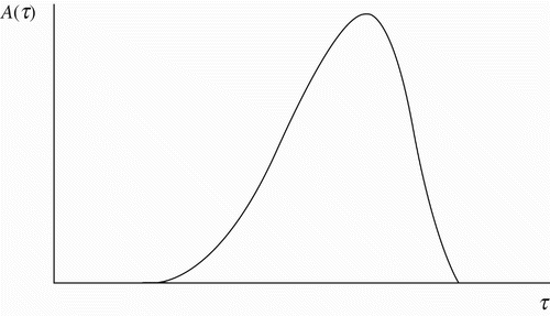
Figure 1. A typical infectivity function A(τ).

In order to be mathematically precise, we assume

Our aim is now to derive a general conclusion from Equations (1) and (2). To do so, we introduce the cumulative force of infection

By integrating Equation (1) from −∞ to t, interchanging the order of the integrals and using

and then Equation (2), we obtain the scalar nonlinear renewal equation

(note, incidentally, that Equation (4) is of convolution type, whereas Equation (1), with Equation (2) inserted, is not). Since F≥0, we know that y should be an increasing function of t and with a little bit of effort one can check that the rule for extension (4) does indeed preserve this property; that is, if y is increasing on (−∞, 0), then y is increasing on (0,+∞) 11. Moreover, since for y≥0 and A is integrable, y is bounded. So, the limit exists. Using again the integrability of A, one shows that y(∞) has to satisfy the equation

where

can be interpreted as the expected number of secondary cases caused by a primary case introduced in a population with susceptible density S(−∞) or, in the standard jargon, R ₀ is the basic reproduction ratio.

Using elementary properties of the function and simple graphical arguments, one proves that Equation (5) has a unique strictly positive solution if R ₀>1 and no strictly positive solution if R ₀≤1. In order to translate this information into the Kermack–McKendrick threshold theorem, we first observe that Equation (2) implies

where the left-hand side represents the final size of the epidemic, that is, the fraction of the population that is infected, sooner or later, during an outbreak. (See Chapters 18–20 in 51 for an encompassing discussion of the final size equation. And see Appendix B in 47 as well as 2 7 for multi-type generalizations.) Thus, we are led to conclude that

	(i) when R 0>1, introduction of the infective agent leads to an outbreak with the final size given by Equation (7), where y(∞) is the strictly positive solution of Equation (5)
	(ii) when R 0≤1, introduction of the infective agent leads to an outbreak with the final size close to zero.

But several comments are essential for both the derivation of this conclusion and its interpretation:

Concerning (i): this is the deterministic formulation that takes as a starting point that a small but positive fraction of the large population is infected. When we start with a small number of infected individuals, we should describe the initial stages by a branching process. The condition R ₀>1 then amounts to the branching process being supercritical. As a branching process may go extinct, even when supercritical, we may get a minor outbreak. Equation (7) describes the expected size of a major outbreak. See, for instance, the textbook of Diekmann and Heesterbeek 13.

Concerning (ii): for R ₀≤1, the relevant solution of Equation (7) is zero, so where does the ‘close to zero’ come from? In deriving Equation (5), we assumed that y satisfied Equation (4) for all . When providing an initial condition that captures the introduction of a small number of infectives, we essentially replace Equation (4) by

where f(t) is a given function. Thus, we obtain

and conclusion (ii) should be read as follows:

(ii′) when R 0≤1, the positive solution y(∞) of Equation (9) converges to zero when .

See Exercise 1.12.iv in 13 or 51 for details.

If transmission occurs on a time scale which is fast relative to the time scale of demographic changes (birth, death and migration), we may conceive the host population as static during the outbreak. If, moreover, infection confers permanent immunity, the fraction of the population that is susceptible necessarily decreases monotonically and the concept of ‘final size’ makes sense. In this section, we have shown that the expected final size can be characterized in terms of the scalar equation (5) involving only one parameter, the basic reproduction number R ₀. In turn, R ₀ is defined by Equation (6), that is, as the product of the original density of susceptibles and the expected total contribution to the force of infection of one newly infected individual. Equation (5) was derived from a nonlinear scalar renewal equation. The entire content of this section is presented in the 1927 paper of Kermack–McKendrick! The only thing we have done is to rewrite the derivation in such a way that the transition to the next sections, dealing with demographic turnover and with waning immunity, is as smooth as possible.

3. The endemic balance

Even if individuals remain immune for the rest of their life after an infection, new susceptibles arise as a result of reproduction. In this section, we consider the situation where, at the population level, there is a constant birth rate B. So from the point of view of the infectious agent, there is a constant inflow at rate B of ‘resource’.

Individuals come and go: we now also need to specify how long would newborn individuals live. We do so in terms of the probability that an individual stays alive for at least a units of time (see 20 for a very early use of this description in terms of ℱ in the context of an epidemic model). In particular, we assume that this survival probability does not depend on whether or not the individual becomes infected (so we investigate the influence of demographic turnover on disease transmission and not the influence of a deadly infectious disease such as HIV on population dynamics). We would like to keep ℱ general and not restrict to the special family with μ>0, simply since in modern developed countries the observed ℱ is hugely different from exponential. Note that we have introduced two more model ingredients (on top of A(τ)), viz., B and . We assume that , that ℱ is monotonically non-increasing and that exponentially for . We consider B>0.

If no infectious disease is circulating, we observe the stable age distribution

where S is now the number of susceptibles per unit of area and age. If we assume that ‘age’ has no impact on susceptibility or on the force of infection that an individual experiences, we obtain

when F(t) is the prevailing force of infection at time t (indeed, an individual that has age a at time t experienced a force of infection at age σ). If we substitute Equation (10) into

we, exactly as before, express the incidence in terms of past values of the force of infection. Instead of the constitutive equation (1), we now postulate

since we interpret A as an expected contribution given survival, and so the true expected contribution has the conditional survival probability as an extra factor.

If we substitute Equation (10) into Equation (11), we arrive at a nonlinear scalar renewal equation for the unknown F. Apart from the disease-free state F(t)≡0, there might be an endemic steady state. To find it, we need to solve

The right-hand side is a monotonically decreasing function of F, converging to zero for . So, if we assume that the value at F=0, which we denote by R ₀ (since it is indeed the expected number of secondary cases caused by a primary case introduced in a susceptible population with age distribution ), exceeds one, there exists exactly one steady endemic force of infection. And if R ₀<1, no such steady endemic force of infection exists.

The Principle of Exchange of Stability 37 guarantees that the endemic steady state is stable for R ₀ slightly greater than one. To ascertain the local stability for larger values of R ₀, we linearize (11)–(10) and look for solutions of the form for the linearized equation

This leads to the characteristic equation

with F being the unique positive solution of Equation (12) for R ₀>1. It is an open problem to determine whether or not Equation (13) has solutions with for general ℱ. Remarkably, we can show that when , all roots satisfy (for any non-negative and integrable function A!).

Notation: Ā is the Laplace transform of A, that is, .

Theorem 3.1

Assume that with μ>0 and that R ₀>1 where

The solution

of (12) is locally asymptotically stable as a steady state of (11)–(10).

Proof

By the theory developed in 12 16, it suffices to show that all roots of Equation (13) have a negative real part. A straightforward computation, using also Equation (14), shows that Equation (13) takes the form

when . Since (recall that )

and for

the absolute value of the second factor on the right-hand side is bounded above by one. Since R ₀>1, we have

for and hence

So for , the right-hand side of Equation (15) is in absolute value less than one and consequently (15) cannot hold for such λ.   ▪

Remark

The proof given above is a much simplified version of the elaboration of [Exercise 3.10]13. See [Theorem 5]52 for a different proof and various generalizations. Global stability has been shown in 42 and a text-book version of that proof can be found in [Section 9.9]49.

In this section, we have shown that when demographic turnover is described by a constant population birth rate and a general survival function, we can still capture the infectious disease dynamics by a scalar renewal equation for the force of infection. This equation has a positive steady state if and only if R ₀>1 and there is at most one such steady state. For the special case of a constant per capita death rate, we can find that this steady state is locally asymptotically stable. Whether or not it is for general survival is an open problem. But note that Andreasen 1, Magal and Ruan 43 and Thieme 50 found that instability is certainly possible if we allow the susceptibility or the infectiousness of an individual to depend on its age.

4. Waning immunity

When immunity reduces susceptibility, but has no impact on infectiousness once the infection occurs, we can stick to the already introduced A(τ) to describe the expected contribution to the force of infection at time τ after infection, given survival.

There are at least two ways to describe temporary partial immunity. One may assume that all individuals, at time τ after the last infection took place, have their susceptibility reduced by a factor Q(τ), meaning that the probability of getting infected upon contact with an infectious individual is Q(τ) times what it is for a fully susceptible individual (so Q(τ)=0 corresponds to full protection and Q(τ)=1 to full susceptibility). Another possibility is to allow only for full protection or full susceptibility and to describe the probability that at time τ after the last infection an individual is fully susceptible again by P(τ). Note that SIS and SIRS compartment models (see Appendix) are of this type. Note that Inaba 28–30 followed Kermack and McKendrick 32 33 35 36 in assuming that a new clock starts when an event transforms an infected individual into a recovered individual and that the reduction in susceptibility is a function of the time shown by the second clock (see 54 for a similar approach; also see 18 43 46 53). Also note that one can, of course, introduce a compartment of intermediate protection (see e.g. 39 48 and the references given there) and thus obtain a description that combines features of both gradual return of susceptibility and variability in the length of the time window of protection. One might also assume that susceptibility does not simply depend on the time since last infection, but also depends on the history of previous infections 39.

Note that we have to make sure that an infected individual that contributes to the positivity of P(τ) should not contribute to the positivity of A(σ) for , as otherwise the possibility of re-infection does have an influence on expected infectiousness (for compartmental models of SIS and SIRS type, etc., this is indeed guaranteed). When we work with Q, the safest assumption is to require that Q(τ)=0 for . In any case, we can assume that Equation (11), which we repeat here as

remains valid, interpreting (in case of reduced susceptibility) S(t, a) in terms of susceptible equivalents, in the sense that one individual with reduced susceptibility Q(τ) is counted as Q(τ) susceptibles. But we have to change expression (10) for the number of susceptibles per unit of area and age, in order to account for regained susceptibility (long) after infection.

Another important observation is that, implicitly, P and Q refer to an individual while conditioning that this individual is not yet re-infected. The possibility of re-infection leads, in the case of partial susceptibility, to the conclusion that of the individuals that become infected at time t−τ, a fraction

will not have been re-infected before time t. If we work in the P-framework and consider again an individual infected at time t−τ, the probability that it is susceptible at time t is given by the Stieltjes integral:

(indeed, if the individual regains full susceptibility at time σ after infection, it has to escape from re-infection on a time interval of length τ−σ beginning at ). These observations motivate us to define

in order to capture Q-models and P-models in one uniform notation. Here, we use the notational convention

of the theory of delay equations 15 21.

We are now ready to replace expression (10) by the equation

Thus, the model is described by the two equations (16) and (19) for the two unknowns F(t) and S(t, a) and it has as its ingredients B, , A(τ) and either Q(τ) or P(τ). For a given F, Equation (19) is linear in S, so solving Equation (19) is in principle straightforward, and upon substitution of the result into Equation (16), we end up with a scalar nonlinear renewal equation for F. In fact, one can solve Equation (19) by successive approximation, which amounts to generation expansion: the term corresponds to individuals that have never been infected and the next term

to individuals that have been infected once, etc. Whenever the support of Q or P is bounded away from zero (meaning that the time window between two successive infections has a strictly positive minimal length), there are, at any given finite age, only finitely many non-zero terms in the generation expansion. So, if in addition for any , we find in this way an exact representation of the solution of Equation (19) as a finite sum of explicit expressions involving the history of F. We conclude that the dynamics of an epidemic model that incorporates a general survival function and various quite general forms of waning immunity is still fully described by a scalar nonlinear renewal equation!

If we define q(t, a) by the relation

then q describes the relative susceptibility (Q-version) or the probability to be susceptible ($P$-version) of an individual of age a at time t, given survival. Upon substitution of this relation into Equation (19), we find for q the equation

while substitution into Equation (16) leads to

Clearly, F(t)≡0, corresponds to the disease-free steady state. An endemic steady state is characterized by

The right-hand side of Equation (24) for q(a)≡1 is again equal to R ₀, just as it was in the preceding section (the possibility of re-infection has no impact on R ₀ for the simple reason that when infection is very rare, it can be excluded that the same individual is infected again). If, as before, we solve the linear equation (23) by generation expansion and substitute the result into Equation (24), we obtain the scalar equation from which we have to determine the unknown F>0.

In the special case that , Equation (24) reduces to

Equation (23) is a linear renewal equation, so it can be solved by Laplace transformation, leading to

In the P-version, we have

where P̄(μ) is the Laplace–Stieltjes transform of P:

So for the P-version, we find

and since , the right-hand side is a decreasing function of F. Accordingly, Equation (25) has a unique positive solution whenever R ₀>1 and no such solution when R ₀≤1. We conjecture that the same is true for the Q-version, but so far we did not manage to prove this. We also conjecture that this conclusion holds for general . In order to show this, we might rewrite the factor

in Equation (24) by integration by parts as

(where, for convenience, we have assumed that ℱ is differentiable; since ℱ is anyhow monotone decreasing, the general case can be dealt with by using a Stieltjes integral). Now, note that is the expected time that an individual that survived till age a spent being susceptible (weighed in the appropriate manner when we work with the Q-version). So, it seems very reasonable to conjecture that

(note that q itself may depend in a more complicated way on F, as an increase in F leads first to a decrease of the expected age of the first infection but next to an increase of return to the susceptible class at an early age). It remains to study in detail how the solution of the renewal equation (23) depends on the parameter F.

5. Concluding remarks

Often when epidemic models are formulated as delay equations, the aim is to derive conditions for the (in)stability of the endemic steady state and to find out, by way of the Hopf bifurcation theorem, when one should expect to find persistent oscillations 5 6 10 14,22–26,29 43 55 56.

The trigger for the approach sketched in the present paper is somewhat different: our ultimate goal is to find conditions for strain replacement as a result of mass vaccination 17 19 27 38 44. In this context, the need arises to incorporate

	(i) a realistic form of demographic turnover,
	(ii) the waning of immunity and
	(iii) cross-immunity.

The above text describes our approach for dealing with issues (i) and (ii). We realise that dealing in an effective yet meaningful way with issue (iii) presents a major challenge. Since Simon Levin has considerable expertise in this matter 3 8 9 40, his extremely valuable advice on this matter will be highly appreciated.

Acknowledgements

We are grateful to Horst Thieme for providing us with a substantial list of very relevant references! Comments by Horst and by Hisashi Inaba have been very helpful.

Notes

^†Dedicated to Simon Levin on the occasion of his 70th birthday. Thank you Simon for being an organizing centre for mathematical biology, a source of inspiration for two of the authors for many years.

, , and .

Appendix

Here, we show how the familiar SIS compartmental model described by the ODE system

fits into the framework described in this paper. Hopefully, our presentation is such that the reader is convinced that also models with additional exposed and/or removed compartments, such as the SEIRS model described by

are covered by our approach.

For a given function F=F(t), let M _i (t; s), i=1, 2, be defined by

So, is the first column of the fundamental matrix solution of the linear ODE system generated by the matrix

and if we define

it follows that

Our task is to relate Equation (22) to the equation

that allows us to identify (A5) and (A1). But in order to do so, we need to uncover first the relation between Equation (21) and the definition of M.

By using for each of the two equations of (A3) the variation-of-constants formula, we obtain

and upon substitution of the second of these into the first, we obtain

If we now put and s=t−a, we recover exactly Equation (21) for the special case that (and hence ).

From Equation (A4), we have

and from the variation-of-constants formula, we have

If we insert the second of these into the first and write again , we find upon changing the order of integration

If we now multiply both sides by β and insert and into Equation (22), we find that the right-hand side of Equation (22) coincides with the right-hand side of the identity for β I(t). In other words, starting from Equation (A1), we have derived Equation (22) for F(t) defined by , in the special case that and and with q defined by Equation (21) in the special case that .

References

- Andreasen , V. 1995 . “ Instability in an SIR-model with age-dependent susceptibility ” . In Mathematical Population Dynamics: Analysis of Heterogeneity Volume 1: Theory of Epidemics , Edited by: Arino , O. , Axelrod , D. , Kimmel , M. and Langlais , M. 3 – 14 . Winnipeg : Wuerz Publishing .
- Andreasen , V. 2011 . The final size of an epidemic and its relation to the basic reproduction number . Bull. Math. Biol. , 73 : 2305 – 2321 .
- Andreasen , V. , Lin , J. and Levin , S. A. 1997 . The dynamics of cocirculating influenza strains conferring partial cross-immunity . J. Math. Biol. , 35 : 825 – 842 .
- Bacaër , N. 2012 . The model of Kermack and McKendrick for the plague epidemic in Bombay and the type reproduction number with seasonality . J. Math. Biol. , 64 : 403 – 422 .
- Beretta , E. and Breda , D. 2011 . An SEIR epidemic model with constant latency time and infectious period . Math. Biosci. Eng. , 8 : 931 – 952 .
- Blyuss , K. B. and Kyrychko , Y. N. 2009 . Stability and bifurcations in an epidemic model with varying immunity period . Bull. Math. Biol. , 72 : 490 – 505 .
- Brauer , F. 2012 . Heterogeneous mixing in epidemic models . preprint to appear in Can. Appl. Math. Q.
- Castillo-Chavez , C. , Hethcote , H. W. , Andreasen , V. , Levin , S. A. and Liu , W. M. Cross-immunity in the dynamics of homogeneous and heterogeneous populations . Proceedings of the Autumn Course Research Seminars . 1986 , Trieste . Mathematical Ecology , Edited by: Hallam , T. , Gross , L. and Levin , S. A. pp. 303 – 316 . Singapore : World Scientific .
- Castillo-Chavez , C. , Hethcote , H. W. , Andreasen , V. , Levin , S. A. and Liu , W. M. 1989 . Epidemiological models with age structure, proportionate mixing, and cross-immunity . J. Math. Biol. , 27 : 233 – 258 .
- Cooke , K. L. and Van Den Driessche , P. 1996 . Analysis of an SEIRS epidemic model with two delays . J. Math. Biol. , 35 : 240 – 260 .
- Diekmann , O. 1977 . Limiting behaviour in an epidemic model . NLA-TMA , 1 : 459 – 470 .
- Diekmann , O. and Gyllenberg , M. 2012 . Equations with infinite delay: Blending the abstract and the concrete . J. Differ. Equ. , 252 : 819 – 851 .
- Diekmann , O. and Heesterbeek , J. A.P. 2000 . Mathematical Epidemiology of Infectious Diseases: Model Building, Analysis and Interpretation (Mathematical and Computational Biology) , Chichester : John Wiley .
- Diekmann , O. and Montijn , R. 1982 . Prelude to Hopf bifurcation in an epidemic model: Analysis of a characteristic equation associated with a nonlinear Volterra integral equation . J. Math. Biol. , 14 : 117 – 127 .
- Diekmann , O. , van Gils , S. A. , Verduyn Lunel , S. M. and Walther , H.-O. 1995 . “ Delay Equations: Functional, Complex, and Nonlinear Analysis ” . In Applied Mathematical Sciences , Vol. 110 , Berlin : Springer-Verlag .
- Diekmann , O. , Getto , Ph. and Gyllenberg , M. 2007 . Stability and bifurcation analysis of Volterra functional equations in the light of suns and stars . SIAM J. Math. Anal. , 39 : 1023 – 1069 .
- Dorigatti , I. and Pugliese , A. 2011 . Analysis of a vaccine model with cross-immunity: When can two competing infectious strains coexist? . Math. Biosci. , 234 : 33 – 46 .
- Feng , Z. and Thieme , H. R. 2000 . Endemic models with arbitrarily distributed periods of infection I: Fundamental properties of the model . SIAM J. Appl. Math. , 61 : 803 – 833 .
- Feng , Z. , Iannelli , M. and Milner , F. A. 2002 . A two-strain tuberculosis model with age of infection . SIAM J. Appl. Math. , 62 : 1634 – 1656 .
- Gripenberg , G. 1983 . On a nonlinear integral equation modelling an epidemic in an age-structured population . J. Reine Angew. Math. , 341 : 54 – 67 .
- Hale , J. K. and Verduyn Lunel , S. M. 1993 . “ Introduction to Functional Differential Equations ” . In Applied Mathematical Sciences , Vol. 99 , Berlin : Springer-Verlag .
- Hethcote , H. W. and Levin , S. A. 1989 . Periodicity in epidemiological models. Applied mathematical ecology (Trieste, 1986) . Biomathematics , 18 : 193 – 211 .
- Hethcote , H. W. and Tudor , D. W. 1980 . Integral equation models for endemic infectious diseases . J. Math. Biol. , 9 : 37 – 47 .
- Hethcote , H. W. and Van Den Driessche , P. 1995 . An SIS epidemic model with variable population size and a delay . J. Math. Biol. , 34 : 177 – 194 .
- Hethcote , H. W. , Stech , H. W. and Van Den Driessche , P. 1981 . Nonlinear oscillations in epidemic models . SIAM J. Appl. Math. , 40 : 1 – 9 .
- Huang , G. , Beretta , E. and Takeuchi , Y. 2012 . Global stability for epidemic model with constant latency and infectious periods . Math. Biosci. Eng. , 9 : 297 – 312 .
- Iannelli , M. , Martcheva , M. and Li , X.-Z. 2005 . Strain replacement in an epidemic model with super-infection and perfect vaccination . Math. Biosci. , 195 : 23 – 46 .
- Inaba , H. 1998 . “ Mathematical analysis for an evolutionary epidemic model ” . In Mathematical Models in Medical and Health Sciences , Edited by: Horn , M. A. , Simonett , G. and Webb , G. F. 213 Nashville , TN : Vanderbilt University .
- Inaba , H. 2001 . Kermack and McKendrick revisited: The variable susceptibility model for infectious diseases . Japan J. Indust. Appl. Math. , 18 : 273 – 292 .
- Inaba , H. 2002 . “ Endemic threshold and stability in an evolutionary epidemic model ” . In Mathematical Approaches for Emerging and Reemerging Infectious Diseases: Models, Methods and Theory , Edited by: Castillo-Chavez , C. , Blower , S. , van den Driessche , P. , Kirschner , D. and Yakubu , A.-A. 337 New York : Springer .
- Kermack , W. O. and McKendrick , A. G. 1927 . A contribution to the mathematical theory of epidemics . Proc. R. Soc. Lond. Ser. A , 115 : 700 – 721 .
- Kermack , W. O. and McKendrick , A. G. 1932 . Contributions to the mathematical theory of epidemics-II. The problem of endemicity . Proc. R. Soc. Lond. Ser. A , 138A : 55 – 83 .
- Kermack , W. O. and McKendrick , A. G. 1933 . Contributions to the mathematical theory of epidemics-III. Further studies of the problem of endemicity . Proc. R. Soc. Lond. Ser. A , 141A : 94 – 122 .
- Kermack , W. O. and McKendrick , A. G. 1991 . A contribution to the mathematical theory of epidemics in classics of theoretical biology (part two) . Bull. Math. Biol. , 53 : 33 – 55 .
- Kermack , W. O. and McKendrick , A. G. 1991 . Contributions to the mathematical theory of epidemics-II. The problem of endemicity in classics of theoretical biology (part two) . Bull. Math. Biol. , 53 : 57 – 87 .
- Kermack , W. O. and McKendrick , A. G. 1991 . Contributions to the mathematical theory of epidemics-III. Further studies of the problem of endemicity in classics of theoretical biology (part two) . Bull. Math. Biol. , 53 : 89 – 118 .
- Kielhöfer , H. 2004 . “ Bifurcation Theory: An Introduction with Applications to PDEs ” . In Applied Mathematical Sciences , Vol. 156 , New York : Springer .
- Kryazhimskiy , S. , Dieckmann , U. , Levin , S. A. and Dushoff , J. 2007 . On state-space reduction in multi-strain pathogen models, with an application to antigenic drift in influenza A . PLoS Comput. Biol. , 3 : 1513 – 1525 .
- Lavine , J. S. , King , A. A. and Bjørnstad , O. N. 2011 . Natural immune boosting in pertussis dynamics and the potential for long-term vaccine failure . PNAS , 108 : 7259 – 7264 .
- Lin , J. , Andreasen , V. and Levin , S. A. 1999 . Dynamics of influenza A drift: The linear three-strain model . Math. Biosci. , 162 : 33 – 51 .
- MacDonald , N. 1989 . Biological Delay Systems: Linear Stability Theory , Cambridge : Cambridge University Press .
- Magal , P. , McCluskey , C. C. and Webb , G. F. 2010 . Lyapunov functional and global asymptotic stability for an infection-age model . Appl. Anal. , 89 : 1109 – 1140 .
- Magal , P. and Ruan , S. 2010 . Sustained oscillations in an evolutionary epidemiological model of influenza A drift . Proc. R. Soc. A , 466 : 965 – 992 .
- Martcheva , M. , Iannelli , M. and Li , X.-Z. 2007 . Subthreshold coexistence of strains: The impact of vaccination and mutation . Math. Biosci. Eng. , 4 : 287 – 317 .
- Metz , J. A.J. 1978 . The epidemic in a closed population with all susceptibles equally vulnerable; some results for large susceptible populations and small initial infections . Acta Biotheoretica , 27 : 75 – 123 .
- Pease , C. M. 1987 . An evolutionary epidemiological mechanism, with applications to type A influenza . Theoret. Popul. Biol. , 31 : 422 – 452 .
- Rass , L. and Radcliffe , J. 2003 . Spatial Deterministic Epidemics , Providence , RI : AMS .
- Swart , A. N. , Tomasi , M. , Kretzschmar , M. , Havelaar , A. H. and Diekmann , O. 2012 . The protective effects of temporary immunity under imposed infection pressure . Epidemics , 4 : 43 – 47 .
- Smith , H. L. and Thieme , H. R. 2011 . Dynamical Systems and Population Persistence , Providence , RI : AMS .
- Thieme , H. R. 1991 . “ Stability change of the endemic equilibrium in age-structured models for the spread of SIR type infectious diseases ” . In Differential Equations Models in Biology, Epidemiology and Ecology , Edited by: Busenberg , S. and Martelli , M. 139 – 158 . Berlin : Springer .
- Thieme , H. R. 2003 . Mathematics in Population Biology , Princeton Series in Theoretical and Computational Biology Princeton , NJ : Princeton University Press .
- Thieme , H. R. and Castillo-Chavez , C. 1993 . How may infection-age-dependent infectivity affect the dynamics of HIV/AIDS? . SIAM J. Appl. Math. , 53 : 1447 – 1479 .
- Thieme , H. R. and van den Driessche , P. 1999 . Global stability in cyclic epidemic models with disease fatalities . Fields Inst. Commun. , 21 : 459 – 472 .
- Thieme , H. R. and Yang , J. 2002 . An endemic model with variable re-infection rate and application to influenza . Math. Biosci. , 180 : 207 – 235 .
- Thieme , H. R. , Tridane , A. and Kuang , Y. 2008 . An epidemic model with post-contact prophylaxis of distributed length. I. Thresholds for disease persistence and extinction . J. Biol. Dyn. , 2 : 221 – 239 .
- Thieme , H. R. , Tridane , A. and Kuang , Y. 2008 . An epidemic model with post-contact prophylaxis of distributed length. II. Stability and oscillations if treatment is fully effective . Math. Model. Nat. Phenom. , 3 : 267 – 293 .