Responses of the haploid-to-diploid ratio of isomorphic biphasic life cycles to time instability

Abstract

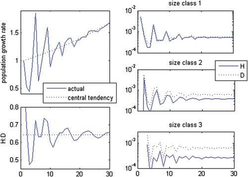
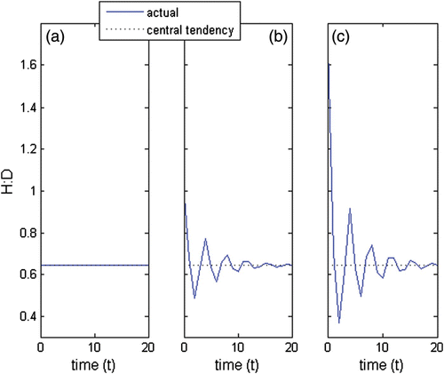
Previous modelling of the haploid-to-diploid ratio (H:D) in biphasic life cycles relied on estimates of the stable population growth rate and structure. This is a projective analysis that estimates the population dynamics given current conditions. However, the environment is rarely constant and has both periodicity and random instabilities. The objective of this work was to unveil how the H:D responds to them. It was found that ploidy phase dissimilarities on the demographic matrix and/or in the initial population structure cause an inevitable H:D time variability as a consequence of the life-cycle structure and independent of the environmental seasonal cycle. This variability depends on the type of life strategy, demographic processes involved and ploidy dissimilar vital rates. Furthermore, ploidy dissimilar fertility or growth rates cause cyclic oscillations mismatching the seasonal cycle, whereas ploidy dissimilarities in the ramet looping rates (survival related) induce a monotonical variation.

Keywords:

• biphasic life cycle
• G:T
• H:D
• time variability
• transient dynamics

MSC2010:

• 91D20
• 65F15

1. Introduction

The majority of the more evolved life forms have diploid life cycles. Such is the case of animals, most of the plants and many protists. Yet, it has not always been so. Plants first appeared about 500 m.y.a during the Palaeozoic era, Cambrian period. These were non-vascular plants (earlier bryophytes) having haploid life cycles, which have persisted until now. The earlier vascular plants emerged about 400 m.y.a during the Devonian period. These had haploid–diploid (biphasic) life cycles, that is, alternated between haploid and diploid generations. It is considered to be a generation when cells replicate suffering mitotic divisions and are able to sustain on their own. The earlier vascular plants became extinct about 200 m.y.a during the Mesozoic era and late Triassic early Jurassic period. These were replaced by the modern vascular plants with diploid life cycles. Although absent in animals and plants, biphasic life cycles prevail in some fungi and many protists. A few modelling-based theoretical studies propose biphasy advantages that may sustain the prevalence of such life cycles 11 12 18. In kelp (brown algae), the haploid (microscopic) and diploid (macroscopic) phases are heteromorphic, whereas in red algae the distinct ploidy phases seem to be isomorphic.

Most of the analyses of demographic models of haploid–diploid life cycles have focused on the stable population growth and structure 7 11 12 18 23 29 33 34. These are projections of the population structure at steady state if the vital rates remain unchanged. These are very helpful in determining the key aspects governing the populations’ dynamics but must not be confounded with forecasting. This is the case of the analyses carried out to determine as to why the haploid-to-diploid ratio (H:D) of a large number of species with isomorphic biphasic life cycles varies, when phases are expected to be ecologically undifferentiated 6 7 29 33 34. Vieira and Santos 33 determined several key aspects of the H:D dynamics: (i) the vital rates should be classified as fertility, growth and looping types, the latter grouping stasis, breakage and clonal growth (i.e. cycling in the same ploidy); (ii) life strategies could be classified as those of investment in fertility, growth or looping; and (iii) the H:D is particularly responsive to ploidy phase dissimilarities in looping. Hughes and Otto 12 also relied on steady-state population analysis to determine whether biphasic life-cycle species must conditionally differentiate their haploid and diploid phases for biphasy to prevail. Conditional differentiation means separate entities differentiating the way they adapt to the environment in order to coexist, implying that if one is better at something, the other is better at something else. During the last few decades, much evidence that haploids and diploids of isomorphic biphasic life cycles conditionally differentiate morphologically and/or physiologically has emerged, implying ploidy dissimilarities in the related vital rates 2 4 9 10 13 16 17 19 20 24 26 27 30 32.

In demographic models, provided that the life cycle is irreducible, that is, all the stages contribute to at least one other stage, and that the transitions among stages do not vary with time or density, the population will approach asymptotically stable structure and growth rate 3. Until then, its trajectory will generally oscillate around a central tendency given by the asymptotic stable trajectory. It is the transient phase during which the population trajectory and dynamics are determined both by the life-cycle properties and by the initial population structure 3. An H:D time variability has been documented in seaweed species 5 6 15 25 26 28, possibly resulting from conditional differentiation of ploidy phases in seasonal environments. Even under weak seasonality, the environment is subject to the sporadic occurrence of extreme events. Most often, the time-variant environment may be expected to drive a natural population from one transient phase to another. Therefore, it is reasonable to expect populations of biphasic life-cycle algae species to endure for more time at an unstable transient trajectory than at a stable one, highlighting the relevance of understanding its dynamics.

The main questions investigated in this work are ‘How may dissimilarities between ploidy phases drive an H:D variability under transient conditions?’ and ‘How does variability relate to the different life strategies, that is, those dominated by fertility, growth or looping?’. To answer these questions, the H:D variability was simulated using models previously developed by Vieira and Santos 33 34. It was tested for the effects of ploidy uneven initial population structures and a ploidy conditional differentiation of the fertility, growth and looping rates. The oscillatory properties of the transient phase of the H:D such as its duration, wave amplitude and wave length were then analysed and related to the three basic life strategies, that is, those dominated by fertility, growth or looping.

2. Methods

2.1. The matrix demographic model

The model used in this study is based on the biphasic life-cycle, stage/size-structured model previously used by Vieira and Santos 33. It is a simplification of a life cycle that is actually triphasic. Under the assumption the sex ratio is approximately constant and the male gametophytes always produce enough spores to fertilize all the females, the carposporophyte phase may be neglected. Hence, the model turns biphasic with the carpospores being considered the output of the gametophyte fecundity. It is a ramet-based model, meaning that the units of the adult stages are the individual fronds that may rise from the same holdfast. It is a deterministic demographic model with a projection interval of one month represented by the eight-dimensional population vector and the (8,8)-dimensional population matrix (Equation (1)). The haploids were separated into tetraspores and gametophyte ramet stages (size classes) ‘1’, ‘2’ and ‘3’, whereas the diploids were separated into carpospores and tetrasporophyte ramet stages ‘4’, ‘5’ and ‘6’. The growth vital rates (g), the looping vital rates (l) and the spore survival (ss) are probabilities and hence vary between 0 and 1. The g and l rates of each stage add up to survival, which cannot be higher than 1. The model considered two ways by which a ramet may loop back: it may stay in the same size class (stasis) or it may break to a smaller size class. The probability of stasis was considered to be 0.75×l for size classes 2 and 3, whereas the probability of breakage to smaller stages was the remaining 0.25×l. These probabilities were based on the analysis of the vital rates of the red seaweed Gelidium sesquipedale 21. It was verified that the model results were not significantly altered when other probabilities were considered. The fecundity transitions (fec _x ) are spore production rates and hence could theoretically vary between 0 and +∞. The ploidy dissimilarities in fecundity, growth and looping rates were introduced by the coefficients d _F , d _g and d _l , respectively, representing the proportion of diploid vital rates relative to the haploid:

Several thousands of different demographic matrices were assembled by choosing their entries under the following conditions:

•	Fecundities (i.e. spore production) were given a fixed value of 100 to the smaller size class, of 500 to the medium one and of 1000 to the larger one. The values themselves were chosen arbitrarily with the sole objective of reflecting that fecundity increases exponentially with the ramet size. Still, care was taken to keep the values of the fecundities simple yet close to the values observed by Santos and Nyman [21 .
•	Spore survival (ss) could range from 10−6 to 100. These encompass the spore survival range observed for most seaweeds and were further expanded to the highest survival possible . Testing a wide range of spore survival was fundamental because the H:D dynamics varies extremely with the amount of fertility output [7,33,34 .
•	Growth (g) and looping (l) could range from 0 to 1. These were chosen to test the vital rates in a wide range of values.
•	The dissimilarity coefficients d F , d G and d L were tested for values between 0 and 2; that is, the diploid vital rates were from 0% to 200% of the haploid vital rates. Still, only over the fertility rates may reasonably be expected the occurrence of ploidy dissimilarities largely different from 100%. Therefore, only over d F were tested values largely different from 1.

Many of the demographic matrices obtained were widely different from reality. To select only the credible ones, two extra criteria were followed: (i) the asymptotic population growth rate (λ) could not be lower than 1 as this corresponds to populations going extinct and (ii) λ could not be higher than 1.1 as this corresponds to demographic burst (at a 1-month projection interval). λ was estimated as the dominant eigenvalue extracted from the demographic matrix 3.

The selected demographic matrices were plotted in a ternary plot (also called triangular plot or triplot) of the elasticities of λ to fertility, growth and looping parameters as proposed by Caswell 3, Franco and Silvertone 8 and Oostermeijer et al. 14. The populations much more elastic to only one type of vital rates are located closer to the respective vertices of the triangle. It is an estimator of the type of life strategy 3 8 14 33 34.

Ploidy dissimilarities in the initial population structure were imposed by the dissimilarity coefficients d _S , d ₁, d ₂ and d ₃, setting the proportionality between the haploid and diploid initial abundances.

2.2. Analytical solution of the transient phase

The population's structure and abundance at a given time t are given by the vector N _t , which is a function of the eigenvalues (λ _i ) and eigenvectors (w _i ) extracted from the respective demographic matrix and the coefficients for the initial conditions (c _i ):

λ, w and c have two possible forms: as a strictly real set or as a set of complex conjugated pairs. In the first case, they can be written exactly as in Equation (2) or transposed to polar coordinates where and . In the latter case, the complex conjugated pair (Equation (3a)) can be rearranged with the eigenvectors and c coefficients in Cartesian coordinates or in polar coordinates (Equation (3b)), where λ and θ are the ith eigenvalue's module and angle, γ and ρ are, respectively, the c _i coefficient's module and angle, and σ and ω _j are the module and angle of the eigenvector's entry w _ji :

The demographic transient dynamics was assessed from the sub-dominant eigenvalues and eigenvectors and from the c coefficients. The sub-dominant eigenvalues are the biases from the central tendency of the population growth rate and the sub-dominant eigenvectors are the biases from the central tendency of the population structure. The central tendency is given by the dominant eigenvalue and eigenvector. Thus, their knowledge is also fundamental for the analysis of the transient phase. The c coefficients enable the initial population vector (N ₀) to be written as a linear combination of the eigenvectors 3. This can be seen if time t is set to 0 in Equation (2). Therefore, the c coefficients also give the initial momentum of their eigenvectors (and associated biases). These initial momentums were converted to the relative initial momentums. Their formulas were for the real sets and for the complex conjugate sets. Their rate of persistence through time was estimated as , where λ _b is a sub-dominant eigenvalue, whereas λ _a is the dominant eigenvalue. This is the inverse of the damping ratio proposed by Caswell 3. The persistence rate shows the rate at which the initial momentum persists, and thus the higher it is, the longer the population is at its transient phase. The oscillatory properties of the transient trajectories were fully defined by the eigenvalues (for the persistence rate), eigenvectors (for the population structure) and c coefficients (for the initial momentum). In Appendix 1, a detailed explanation of these metrics and how they interact to yield a determined transient trajectory of the population growth rate and H:D is given.

2.3. Responsiveness analysis

We evaluated how responsive the oscillatory properties of the transient trajectory to dissimilarities between ploidy phases were. This was done by estimating the following:

•	Elasticity of the persistence rate.
•	Elasticities of the phase ratios within the eigenvector . The amplitudes of the oscillations of each stage were given by the respective entry in the eigenvector. Yet, it was more feasible and interesting to test and present the ratio between the amplitudes of the ploidy correspondent stages.
•	Sensitivity of the relative initial momentum. In the absence of any kind of ploidy dissimilarities, some γ diverged from zero only at very low decimal places and it was due to precision error. These elasticities were automatically set aside as they required this value in the denominator.

The elasticities and sensitivities to the ploidy phase dissimilarities in the demographic matrix (d _F , d _G and d _L ) and in each stage of the initial population vector (d _S , d ₁, d ₂ and d ₃) were estimated by changing these independent variables by 0.01 from an initial value of 1 (i.e. no dissimilarities). The initial population vector was always .

3. Results

The demographic matrices were represented in the triangular plot using their relative elasticities of λ to f, g and l as coordinates and giving a colour scale to the persistence rates of the sub-dominant eigenvalue (Figure 1). It can be seen that both fertility and survival life strategies (respectively, in the F and L lower corners of the triangle) had high persistence rates. Therefore, any population with one of these strategies was subject to long transient phases. There were no demographic matrices with growth life strategies. However, closer to the upper horizontal edge where the growth relevance was higher, the transient phase was also long. This area was considered the growth domain. Separating the F, G and L domains, there was a well-marked area of lower persistence rates and thus short transient phases. In this area were the populations dominated by demographies between fertility and looping. Each domain was associated with a different sub-dominant set of eigenvalue, eigenvector and c coefficient (Figure 2). So, the three types of life strategies had different transient phase characteristics with different responses to dissimilarities among life-cycle phases.

Figure 1. Overall persistence rate (colour scale) plotted upon the triangular ordination of the λ elasticities to fertility (F), growth (G) and looping (L). The coordinate of a point in each axis is given by a line parallel to the lines that intercept the axis coming from its right side.

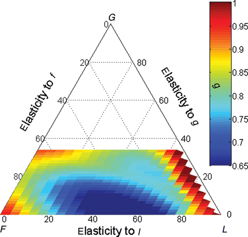
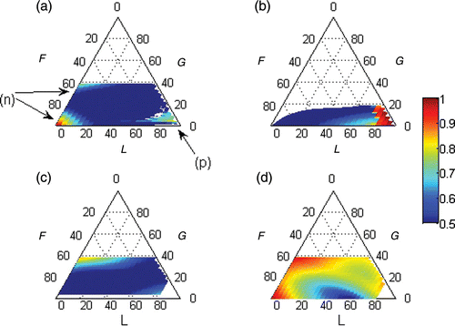
Figure 2. Persistence rates (colour scale) of the specified sets plotted upon the triangular ordination of the λ elasticities to F, G and L. The coordinate in each axis is given by a line parallel to the lines that intercept the axis coming from its right side. (a) Real and equal set, (b) real and symmetric set, (c) complex conjugate and equal set and (d) complex conjugate and symmetric set. The (a) with (n) a negative eigenvalue and (p) a positive eigenvalue.

3.1. Sub-dominant sets of eigenvalues, eigenvectors and c coefficients

The dominant eigenvalue, eigenvector and c coefficient were always strictly real and positive. This was expected from an irreducible primitive life cycle. Moreover, there were typically four types of sub-dominant sets determining the duration, wave amplitude and wave length of the transient population trajectory. One of the ways to characterize them was as either strictly real or complex conjugated pairs. The other way was according to the eigenvector's equality (ploidy balanced) or symmetricity (ploidy unbalanced) of signs for the correspondent stage/size classes of both ploidies (w _i and w _i+4 in Equations (2) and (3)). As to what type of sets did occur, which was the sub-dominant one, how fast did these fade way and which were their oscillatory characteristics depended on the type of life strategy and the magnitude of the ecological dissimilarity between ploidy phases. As an example, a ploidy-balanced population structure could not be given by a linear combination containing ploidy-unbalanced eigenvectors. On the other hand, a ploidy-unbalanced population structure could hardly be given by a linear combination exclusively of eigenvectors tending to be ploidy balanced. Therefore, with ploidy dissimilarities, the equal sets reduced their relative initial momentums, while the symmetric sets increased them. The four possible types of sets are as follows.

3.1.1. Real and equal

This was a set of a strictly real eigenvalue, eigenvector and c coefficient (e.g. Equations (A1a–A1c) in Appendix 2). The eigenvector was equal for the correspondent stage/size classes of both ploidy phases of the life cycle and thus . The eigenvalue could be positive or negative, splitting the set into two sub-types.

3.1.1.1 With a negative eigenvalue.

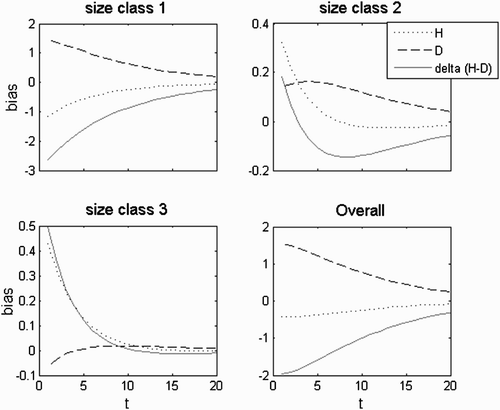
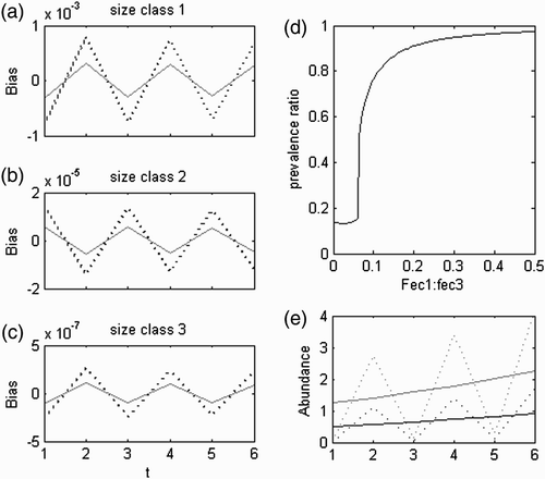
This was only important in the fertility domain (Figure 2(a)). The eigenvector alternated between positive and negative signs for the consecutive stages within each ploidy (Equation (A1) in Appendix 2) with the same periodicity of 2 of its eigenvalue. So, each stage also alternated between benefit and detriment with the same period. This set simulated pulses of individuals from spores to bigger ramets (Figure 3(a–c)) caused by the most immediate production of offspring. This is the shortest, fastest path of growing to the first size class and immediately to reproduce, resulting in a loop with four transitions taking four time steps (4t) to revolve. However, as each ploidy started with its own offspring, there were two simultaneous symmetric pulses resulting in an oscillation with half the period. These pulses were more prevailing the higher the relative fecundities of the smaller size classes were (Figure 3(d)). Ploidy dissimilarities brought a bias between complementary entries in the eigenvector , giving a ploidy an oscillation with a wider amplitude (Figure 3(a–c)). However, its linear combination with the dominant set resulted in ploidy abundances always keeping the same proportionality (Figure 3(e)) and so the H:D did not vary.

Figure 3. Real equal set with a negative eigenvalue. In (a–c), the black solid line represents haploids and the blue dotted line represents diploids. The bias in each size class was standardized to the bias in the spores. In (e), the black lines represent haploids, the blue lines represent diploids, the solid lines represent the central tendency given by the dominant set and the dotted lines represent the linear combination of the dominant set and the real and equal set.

3.1.1.2 With a positive eigenvalue.

This was of only moderate importance in the looping domain (Figure 2(a)) and did not produce any periodic alternation in the bias (θ=0). It simply faded away monotonically with time. Ecological dissimilarities produced a bias always benefiting the abundance of the same ploidy. This was always the same as that favoured by the dominant set and it was always favoured in the same amount.

3.1.2. Real and symmetric

This was only relevant in the looping domain, where it had a very high persistence rate (Figure 2(b)). This was a set with a strictly real eigenvalue, eigenvector and c coefficient (e.g. Equation (A2) in Appendix 2). The eigenvalue was always positive (θ=0) and the eigenvector had symmetrical signs for the correspondent stage/size classes of both ploidies . This produced a bias from the central tendency that permanently favoured a ploidy in detriment of the other. Under ecological similarity, . However, the c coefficient was null (γ=0) and so this set was obsolete (it was switched off). With phase dissimilarities either on the demographic matrix or in the initial population vector, both and the c coefficient became non-null , bringing a momentum (switching on) to the set responsible for a monotonical transition to stability (Figure 4). Often, more of these sets occurred with lesser relevance but still enough to eventually make the transition non-monotonical (as was the case of size class 3 in Figure 4). The linear combination of the real symmetric sets simulated the ploidy uneven component of the slow diffusive flow of individuals through the population structure.

Figure 4. Trajectory of the linear combination of the real symmetric sets. Simulation in the looping domain with i=−3.8, g=0.05 and l=0.96. Dissimilar L with d _L =0.9. λ _b /λ _a =0.88, λ _c /λ _a =0.76, λ _d /λ _a =0.67. γ _a /∑ γ _i =0.095, γ _b /∑ γ _i =0.093, γ _c /∑ γ _i =0.172, γ _d /∑ γ _i =0.253.

3.1.3. Complex conjugate and equal

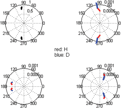
This was very important in the growth domain where it showed a high persistence rate and less important in the looping domain (Figure 2(c)). It was a set of a complex conjugate pair of eigenvalues, eigenvectors and c coefficients (e.g. Equation (A3) in Appendix 2). The eigenvectors were similar for the correspondent stage/size classes of both ploidies. When the pairs were added, they yielded a strictly real set in the form of Equation (3b) preserving the equality of signs between correspondent stage/size classes . It produced a bias that alternated in favouring some size classes in detriment to the others, thus simulating pulses of individuals from spores to the bigger ramets. These pulses were caused by the bulk production of offspring, that is, growing to the larger, more fecund ramets and, once there, to reproduce. However, reproduction was not restricted to the biggest ramet size class and thus the average breeder was slightly below 3 ramet size units and the average number of transitions in the bulk loop was slightly below 8, taking slightly below eight time steps (8t) for the loop to revolve. There were two symmetric loops, each starting in its ploidy, generating individuals in two simultaneous pulses, resulting in an oscillation with half the period (Figure 5). This periodicity was simulated by an eigenvalue with an angle θ in the complex plane of approximately ±π/2 (Figure 6). The more concentrated the fecundities were in one size class, the higher the persistence rate of the pulses , as individuals diffused less through other paths. The more the initial population was concentrated in one size class, the bigger the relative initial momentum of the pulses . σ _i and σ _i+4 were always approximate despite the amount of dissimilarities between ploidy phases (Figure 6). Hence, the amplitudes of the pulses were always very close between the haploid and diploid population structures (Figure 5). Thus, this set was only competent for simulating the ploidy analogous component of the pulses. The eigenvalues, eigenvectors and c coefficients responded to ploidy dissimilarities changing the absolute value of their entries (λ, σ and γ), while their angle in the complex plane (θ, ω _i and ρ) exhibited insignificant differences (Figure 6, but not shown for the c coefficients). Thus, ploidy dissimilarities change the initial momentum, prevalence rate and amplitude of the pulses but not their period.

Figure 5. Bias to the central tendency given by the complex conjugate equal pair of eigenvectors, eigenvalues and c coefficients. Simulation in the growth domain with i=−3, g=0.8 and l=0. This was the demographic matrix with the highest elasticity to G. Dissimilar G with d _G =0.8. Persistence rate=0.84.

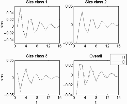
Figure 6. Polar plots of the complex conjugate equal pair of eigenvectors and eigenvalues. In the eigenvalue are plotted λ _b and θ _b , whereas in size class ‘i’ are plotted σ _i and ω _i in red and σ _i+4 and ω _i+4 in blue. Simulation in the growth domain with i=−3, g=0.8 and l=0. Dissimilarities tested for d _G from 1 to 0.6 at intervals of 0.02.

3.1.4. Complex conjugate and symmetric

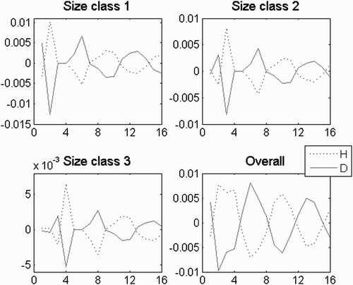
This was particularly important in both the fertility and growth domains. It was also relevant in the transition from the growth to the looping domain (Figure 2(d)). This was a set of a complex conjugated pair of eigenvalues, eigenvectors and c coefficients (e.g. Equation (A4) in Appendix 2). The eigenvectors were symmetric for the correspondent stages of both ploidies. Adding the pairs yielded a strictly real set in the form of Equation 3(b) that preserved the symmetricity of signs between correspondent stages of both ploidies . It produced a bias from the central tendency that alternated in favouring some size classes in detriment to the others, thus simulating pulse flows. However, as the signs of the added eigenvectors’ entries were complementary, the peaks of one ploidy were the sinks of the other (Figure 7). When simulated in the growth domain, the eigenvalues had an angle θ in the complex plane that was half the angle of the complex conjugate equal eigenvalues, thus causing an oscillation with double the period. In this case, the symmetric set was simulating the ploidy unbalance in the pulse flow of individuals through the bulk loop in the life cycle, which is similar to the flow of a single unparalleled pulse. When simulated in the fertility domain, these eigenvalues had an angle θ in the complex plane that was half the angle of the real, equal and negative eigenvalue. In this case, the symmetric set was simulating the ploidy unbalance in the pulse flow of individuals through the shortest loop in the life cycle. So, whatever the life strategy, the ploidy unbalance in the pulse flow was always represented by this symmetric set. Dissimilarities in the vital rates had little effect in the period of the oscillation (the angle of the eigenvalues in the complex plane) but significantly affected its amplitude (σ), initial momentum (γ) and prevalence rate (λ). In particular, in the absence of ploidy dissimilarities in both the demographic matrix and the initial population vector, this set was switched off by a null c coefficient. There were usually two of these sets for a given demographic matrix: one related to the shortest loop in the life cycle and the other related to the bulk loop. As to which started stronger and prevailed further depended on the fertility vs. growth life strategy.

Figure 7. Bias to the central tendency given by the complex conjugate symmetric pair of eigenvectors, eigenvalues and c coefficients. Simulation in the growth domain with i=−3, g=0.8 and l=0.01. This was the accepted demographic matrix with the higher elasticity to G. Dissimilar G with d _G =0.8. Persistence rate= 0.95.

3.2. Systematization of the transient trajectory

The transient trajectory was resumed by the distinct sets representing different flows of individuals (or units) through the population structure. These were either slow diffusive flows or fast pulse flows, through the shortest or the bulk loop of the life cycle, and ploidy balanced or unbalanced. Therefore, the transient trajectory could also be classified by identifying which were the prevailing sets in each life strategy.

3.2.1. Populations in life strategies in the fertility domain

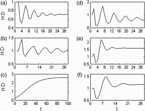
These populations had their transient dynamics dominated by the flow of offspring through the shortest loop in the life cycle. Hence, their short-lasting transient trajectories were characterized by ploidy simultaneous pulses of individuals coming at a short period (2t). The ploidy-balanced component of the pulses was given by the real and equal set. Ploidy dissimilarities either in the life cycle or in the initial population structure gave different amplitudes to the two parallel pulses, resulting in an H:D oscillation with double the period (4t; see Figure 8(a)). This component of the oscillation was given by the complex conjugated symmetric set. The persistence of these pulses was increased by ploidy dissimilarities in fertility rates, but it was reduced by ploidy dissimilarities in growth or looping rates as these enhanced the flow of individuals through other paths. As a matter of fact, the pulse flow of individuals through the longer loop was also present and had a higher prevalence rate. However, it always came with a very low initial momentum, making it meaningless.

Figure 8. H:D transient trajectories with the life strategy in (a) fertility domain with i=−2, g=0.08, l=0.05, d _F =0.5, d _G =1, d _L =1; (b) growth domain with i=−3, g=0.8, l=0.01, d _F =1, d _G =0.8, d _L =1; (c) looping domain with i=−3.8, g=0.8, l=0.96, d _F =1, d _G =1, d _L =0.95, d _spore=4, d ₁=4, d ₂=4 and d ₃=4; (d) between the fertility and the growth domain with i=−2.5, g=0.5, l=0, d _F =0.5, d _G =0.5, d _L =1; (e) between the fertility and the looping domain with i=−2.5, g=0.05, l=0.5, d _F =2, d _G =1, d _L =0.7; and (f) between the growth and the looping domain with i=−3, g=0.3, l=0.5, d _F =1, d _G =1.5, d _L =0.7.

3.2.2. In life strategies in the growth domain

These populations had their transient dynamics dominated by the flow of offspring through the bulk loop in the life cycle. Hence, their long-lasting transient trajectories were characterized by ploidy simultaneous pulses of individuals coming at a big period (4t). The ploidy-balanced component of the pulses was given by the complex conjugate and equal set. Ploidy dissimilarities either in the life cycle or in the initial population structure gave different amplitudes to the two parallel pulses, resulting in an H:D oscillation with double the period (8t; see Figure 8(b)). This component of the oscillation was given by the complex conjugated symmetric set. The initial momentum of the ploidy-unbalanced component of the pulses, the rate at which it prevailed and the amplitude of the H:D oscillations increased with ploidy dissimilarities in fertility or ramet growth rates. Although the transient phase was dominated by the pulse flow through the bulk loop, the first pulse of individuals was through the shortest loop in the life cycle and hence the odd initial oscillation shown in Figure 8(b).

3.2.3. In life strategies in the looping domain

These populations had their transient trajectories dominated by the slow monotonical transition from the initial structure to the stable structure (Figure 8(c)), which originated from the slow diffusion of individuals through the life cycle. This was simulated by the linear combination of the real symmetric sets, the real equal set with a positive eigenvalue and the dominant set. This transient trajectory was extremely responsive to dissimilarities in looping rates and little responsive to anything else. From Figure 8(c), the difference between the dissimilarities imposed in the looping rates and those imposed upon the initial population structure can be observed. A shift in phase dominance (as in Figure 8(c)) could only be attained if the ploidy dominating the initial population structure was opposite to the one dominating the stable population structure. A particular situation occurred when l was decreased slightly and g was increased slightly (e.g. l=0.87 and g=0.1). In these cases, the survival rate was still in the vicinity of 1, and the population was still dominated by looping,but the real sets gave way to the complex conjugated sets. However, these had θ very close to 0 and thus were replacing the real symmetric sets copying their dynamics and role.

3.2.4. In life strategies in the transition from the fertility to the growth domain

In these populations, the pulse flow of individuals through the shorter loop in the life cycle prevailed in the first few instances. However, it soon merged with and gave way to the pulse flow through the main loop. This could be observed from the H:D cycle where an initial period of approximately 4t was gradually overwhelmed by a longer period that asymptotically tended to approximately 8t (Figure 8(d)). However, the amplitude of the oscillations decayed fast and the progression of this shift became veiled.

3.2.5. In life strategies in the transition from the fertility to the looping domain

These populations had the pulse flow of individuals through the shortest loop in the life cycle merged with the slow diffusive flow of individuals throughout the life cycle until its settlement at the stable population structure. It resulted in a short-lasting transient phase with the population attaining its stable structure soon after restart. Therefore, the H:D oscillation with a 4t period also quickly damped away to the H:D at steady state (Figure 8(e)).

3.2.6. In life strategies in the transition from the growth to the looping domain

These populations had the pulse flow of individuals through the bulk loop in the life cycle merged with the slow diffusive flow of individuals throughout the life cycle until its settlement at the stable population structure. It resulted in a short-lasting transient phase with the population attaining its stable structure soon after restart. Therefore, the H:D oscillation with a 8t period also quickly damped away to the H:D at steady state (Figure 8(f)).

4. Discussion

Biphasic life cycles are expected to show an H:D variability in their transient trajectories in the presence of ploidy dissimilarities in the vital rates and/or initial population structure. These are specific to the type of life strategy adopted by the species as they are originated by specific demographic processes. They are also simulated by specific eigenvectors, eigenvalues and c coefficients extracted from the demographic matrix and initial population structure. This H:D variation is exclusively due to the own structure of the life cycle and not related to environmental seasonality, only requiring ploidy dissimilarities in the vital rates and/or in the initial population structure. Even in a generally stable environment, any sporadic instability in the population structure flows through the life cycle, in fast pulses and/or slowly diffusing, generating H:D time variability. Thus, a cyclic time variation of the H:D in a particular population, as observed by Thornber and Gaines 28, cannot be automatically taken as evidence of seasonality. Likewise, a change in the H:D over a period of 12 years 25 should not be immediately taken as evidence that the population is evolving to a new situation.

Dissimilarities between ploidy phases were found over the fecundity rates by Santos and Duarte 20, Scrosati et al. 24, Thornber and Gaines 29 and Thornber et al. 30. These could be seasonal, herbivory dependent and could possibly be due to their different cytological processes of gamete/spore production. Dissimilarities between ploidy phases were also found for spore performance by Destombe et al. 4, Garza-Sanchez et al. 9, Gonzalez and Meneses 10, Pacheco-Ruíz et al. 16, Roleda et al. 19 and Scrosati et al. 24 and for ramet growth and survival rates by Destombe et al. 4, Gonzalez and Meneses 10, Pacheco-Ruíz et al. 16, Thornber et al. 30 and Vergés et al. 32, which are possibly due to conditional differentiation. A perturbation in the population structure may occur following environmentally extreme events, extreme grazing or competition events, provided that they affect ploidy phases differently. One particular situation is when the demographic matrix changes, as it implies that the population structure at the time of change is the initial population structure of a new run. There are several ways this situation is likely to occur: it may be a change in the vital rates inside the survival or the fertility sub-block of the demographic matrix, due to seasonality, or it may be reproductive asynchrony of the spore/gamete donor population, which has been already reported for Gelidium sesquipedale 20.

Ploidy dissimilarities in fertility or growth rates are able to create cyclic niche partitions damping away with time. As long as sporadic extreme events occur, even at low frequencies, these ploidy dissimilarities generate over time the niche partition 12 demonstrated necessary for the evolution and stability of biphasic life cycles. On the other hand, ploidy dissimilarities in a particular looping rate alone are not able to do this and need a counter-weight. To support this, in the simulations of looping-dominated life strategies with ploidy dissimilarities imposed over looping rates, a shift in ploidy dominance only occurred when the initial H:D was opposite to the asymptotic H:D. While the latter H:D was imposed by ploidy dissimilarities in looping rates, the former H:D could only be imposed by something else.

Cyclic oscillations promoting the niche partition necessary for the evolution and stability of biphasic life cycles are only possible in the absence of a seasonality affecting the vital rates. This is because the oscillations are induced by the life-cycle structure, resulting in an H:D evolution miss fitted to the environmental cycle. Suppose the environment changes to a situation where a ploidy is fitter than the other because it reproduces or grows better. If the environmental cycle has a periodicity wider than the one imposed by the life-cycle structure, there is only an increase in the average population fitness for a restricted amount of time. After that, the life-cycle structure and not the environment forces the population to shift to the lesser fit ploidy. The population may only come around this problem if the period of the oscillation induced by the life cycle is wider than the seasonality. In such a case, while the seasonal conditions are better for a particular ploidy, the dominance imposed by the life-cycle structure shall always fit. When environmental change occurs, the population starts a new oscillation with the dominance of the better fit ploidy. Awareness about this is fundamental for future theoretical research on the evolution and stability of biphasic life cycles. The outcome of the modelling essays may be strongly dependent on the duration of the life-cycle loops relative to seasonality. This problem should not occur with ploidy dissimilar survival rates. In such a case, the H:D evolution is always directly proportional to the ploidy fitness ratio.

Many species were documented to seasonally shift their H:D and their ploidy dissimilarities or were simply reported to have a time-variable dynamics. Such were the cases of Gracilaria verrucosa 4, Chondrus crispus 24, Chondracanthus chamissoi 10, Gelidium sesquipedale 20, Mazzaella cornucopiae 22, Sarcothalia crispata 15, Pterocladiella capillacea 27, Mazzaella splendens 5, Gelidium pusillum 17, Gracilaria gracilis 13 and Grateloupia turuturu 1, showing that the H:D time variability is worldwide. The H:D of Mazzaella flaccida observed at Piedras Blancas and Vandenberg (Pacific Coast of North America) with a fine temporal resolution 28 exhibited oscillations mismatching the seasonal cycle. At Piedras Blancas, they were slightly shorter, whereas at Vandenberg they were much longer. In the light of the current work, this suggests that ploidy dissimilarities do exist in fertility and/or growth rates. Assuming that these oscillations were imposed by the life-cycle structure and not by seasonality, the overwhelming difference in their periods at both sites must be driven by site-specific sizes of their life-cycle loops. Then, the ramets in Vandenberg should survive more, attain bigger sizes or get sexually mature later relative to those in Piedras Blancas. Thornber and Gaines 29 showed that a higher diploid fecundity was driving the average haploid dominance in Mazzaella flaccida, while their H:D spatial variability could only be explained by differences in mortality rates. Accordingly, Vieira and Santos 34 suggested that only through ploidy dissimilarities in survival may conditional differentiation drive an effective spatial niche partition. This is required for the evolution and stability of biphasic life cycles 12. In such a case, the ploidy dissimilar fecundities should simply be an unavoidable consequence of the differences between meiosis and syngamy with side effects in the H:D averaged over space and in intermittent site-specific H:D transient trajectories. The latter must not be too frequent or the population will often severely depart the structure optimizing niche exploitation.

Acknowledgements

V.M.N.C.S. Vieira was supported by a PhD grant of ‘Fundação para a Ciência e Tecnologia’, SFRH/BD/19339/2004/MS47. The authors thank Carl Sandrock for the ternplot Matlab® scripts freely available on the internet.

Appendix 1. Descriptors of the transient dynamics

The linear combination (linear in the parameters) of the eigenvalues, eigenvectors and c coefficients extracted from the demographic matrix estimates the population vector at any given time t. Hence, these metrics define the properties of the transient trajectory, namely its initial momentum, duration and wave period and amplitude. Most of this is approached in the literature about matrix population dynamics, as are the cases of Caswell 3 and Tuljapurkar and Caswell 31. A brief overview is given in order to better understand the complex dynamics that govern the transient phase and its relationship with the demography of algae with biphasic life cycles.

A1.1. Central tendency

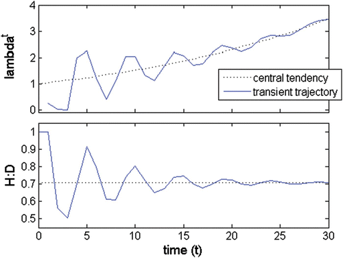
The long-term population dynamics are given by the dominant set; that is, the long-term growth rate tends asymptotically to the dominant eigenvalue and the long-term population structure is given by the eigenvector associated with it. Thus, any statistic from the long-term population structure, as is the H:D, can be estimated upon this eigenvector (Vieira and Santos 2010). As this dominant eigenvalue is strictly real and positive, growth or decline is monotonical and the population structure is stable. During the transient phase, the dominant eigenvalue is the central value around which oscillates the growth rate at a given time t, but it is not its actual rate. Likewise, the associated eigenvector gives the central tendency of the population structure, but it is not its actual structure. Thus, any statistic estimated upon this eigenvector is the central tendency upon which the actual values of the statistic oscillate (Figure A1).

Figure A1. A(a) λ trajectory; (b) H:D trajectory; λ _a =1.042; λ _{b, c} =0.218±0.869i; abs(λ _{b, c} )=0.9; θ _{b, c} =±1.325 rad=±75.9°; wave period=4.74; persistence rate= 0.86.

A1.2. Persistence rate

For each of the sets of eigenvalue, eigenvector and c coefficient, exponential growth or decline depends only on each eigenvalue being bigger or smaller than 1 in absolute value. Relative to the higher eigenvalues, all the smaller eigenvalues tend to turn negligible and thus their influence on the population dynamics fades away (Figure A1). The rate at which the transient phase fades away is commonly measured by the ‘damping ratio’ between the magnitudes of the biggest (dominant) and the second biggest (sub-dominant) eigenvalues . The closer it is to 1 the more the transient phase prevails, but it may raise to +∞. In this work, the statistic was inverted to and named persistence rate. With this inversion, all eigenvalues are scaled to the dominant and their persistence rates are within the 0–1 range. Higher non-dominant eigenvalues, closer to the dominant, have a persistence rate closer to 1 and will take longer to fade away. Moderate non-dominant eigenvalues have a moderate persistence rate and will fade away quicker. Small non-dominant eigenvalues have a persistence rate closer to 0 and will be almost imperceptible. It also enables to estimate the dissipation rate as 1−‘persistence rate’. The persistence rate and the dissipation rate are direct measures of the rate at which it prevails or dissipates the initial momentum (given by the c _i coefficients) of each eigenvector. Therefore, it was fundamental to adopt the persistence rate instead of the damping ratio.

A1.3. Oscillation period

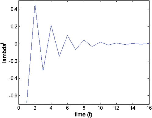
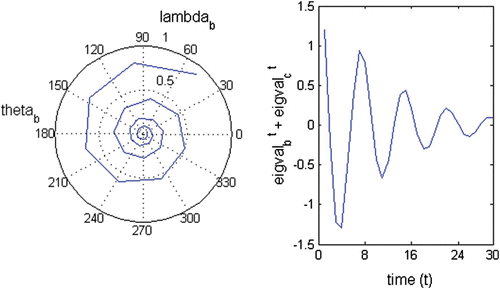
Eigenvalues vary independently as they are raised to time t. Real positive eigenvalues show monotonical exponential growth or decline whether they are bigger or smaller than 1. Real negative eigenvalues oscillate between positive and negative values with a period of 2 (Figure A2). Complex eigenvalues cycle through the complex plane with a period of 2π/θ (Figure A3 (left)). However, complex sets of eigenvalue, eigenvector and c coefficient always come in complex conjugate pairs which, when combined, cancel out their imaginary components. Thus, the sum of the complex conjugate eigenvalues oscillates between strictly real positive and negative values with the same period of 2π/θ (Figure A3 (right)). The oscillation period (or wave length) of the transient trajectory is given by the sub-dominant eigenvalue. Nevertheless, if other eigenvalues have approximate magnitudes, different cycles are over-imposed, leading to an oscillation pattern that resembles a chaotic one.

Figure A2 Oscillatory trajectory of a strictly real negative eigenvalue; λ _b =−0.68; θ _b =180°; wave period= 2.

Figure A3 Oscillatory trajectory of (left) a complex eigenvalue; λ _b =0.598+0.679i; abs(λ _b )=0.905; θ=48.6°; wave period=7.41 and (right) the complex conjugated pair of eigenvalues λ _b and λ _c .

A1.4. Population structure

At any time t, the central tendency of the population structure is given by the eigenvector (w _a ) associated with the dominant eigenvalue (λ _a ), which includes only real, non-negative values. The other eigenvectors (w _i for i≠ a) give the residuals that add up to the central tendency yielding the actual population structure. The sum of the residuals is the wave amplitude. The relative weights of the central tendency and residuals for a given time t are given by . These weights represent the actual momentum of w _i at time t.

The bulk of the oscillatory pattern is given by the sub-dominant set of eigenvector, eigenvalue and c coefficient (or complex conjugated pair of eigenvectors, eigenvalues and c coefficients), whereas the smaller ones may yield smaller, usually undetectable oscillations around the main oscillating trajectory (Figure A1). Nonetheless, several of the biggest non-dominant sets may have approximate absolute values for their eigenvalues, eigenvectors and c coefficients, leading to over-imposed oscillations of close magnitude but different periods (Figure A4). The resulting transient trajectory is odd. However, such statistics like the H:D, by averaging over stage classes, tend to smooth it.

Figure A4 Eigval _a =1.02, λ _a =1.02 and θ _a =0. Eigval _{b, c} =−0.07±0.83i, λ _{b, c} =0.83, persistence rate _bc =0.81, θ _{b, c} =±95.1° and wave period _{(b, c)}=3.79; eigval _d =−0.85, λ _d =0.85, persistence rate _bc =0.83, θ _d =180° and wave period _(d)=2.

Figure A5 H:D when the c coefficients for the complex conjugated pair were multiplied (a) by 0, (b) by 1 and (c) by 2.

A1.5. Initial conditions and momentum

The c coefficients define how much of the initial population structure is explained by each eigenvector. So, by weighting the eigenvalues and eigenvectors, they also weight their influence in the transient phase because the population's trajectory carries a memory of the initial conditions, which fades away as time goes by (Figures A1, A4 and A5). This memory is the momentums that the eigenvectors bear at any particular time. The initial momentum of each eigenvector is given by its c coefficient. The rate at which it grows or decays is given by the correspondent eigenvalue. In relative terms, each relative initial momentum is given by for the real sets or for the complex conjugate sets (see Equation(3)). The rate at which the momentum prevails is given by the persistence rate . Hence, at any time t, the prevailing relative momentum is given by for the real sets and for the complex conjugate sets. In particular situations, there may be a c coefficient close to zero that cancels out its associated eigenvector. If the correspondent eigenvalue is the sub-dominant, it will transfigure the population's trajectory, altering the otherwise expected duration, period and amplitude of the transient phase.

Appendix 2. Common sets of eigenvectors, eigenvalues and c coefficients

Here, examples of the four types of sets of eigenvalues, eigenvectors and c coefficients commonly found for the (8,8)-dimensional demographic matrix of the stage/size-structured model of a biphasic life cycle are given.

A2.1. Real and equal

A2.2. Real and symmetric

A2.3. Complex conjugate and equal

A2.4. Complex conjugate and symmetric

References

- Araújo , R. , Violante , J. , Pereira , R. , Abreu , H. , Arenas , F. and Sousa-Pinto , I. 2011 . Distribution and population dynamics of the introduced seaweed Grateloupia turuturu (Halymeniaceae, Rhodophyta) along the Portuguese coast . Phycologia , 50 ( 4 ) : 392 – 402 .
- Carmona , R. and Santos , R. 2006 . Is there an ecophysiological explanation for the gametophyte-tetrasporophyte ratio in Gelidium sesquipedale (Rhodophyta)? . J. Phycol. , 42 ( 2 ) : 259 – 269 .
- Caswell , H. 2001 . Matrix Population Models: Construction, Analysis and Interpretation , 2 722 Sunderland , , MA, Sinauer Associates
- Destombe , C. , Valero , M. , Vernet , P. and Couvet , D. 1989 . What controls haploid–diploid ratio in the red alga, Gracilaria verrucosa? . J. Evol. Biol. , 2 ( 5 ) : 317 – 338 .
- Dyck , L. J. and DeWreede , R. E. 2006 . Seasonal and spatial patterns of population density in the marine macroalga Mazzaella splendens (Gigartinales, Rhodophyta) . Phycol. Res. , 54 : 21 – 31 .
- Engel , C. , Aberg , P. , Gaggiotti , O. E. , Destombe , C. and Valero , M. 2001 . Population dynamics and stage structure in a haploid–diploid red seaweed, Gracilaria_gracilis . J. Ecol. , 89 ( 3 ) : 436 – 450 .
- Fierst , J. , terHorst , C. , Kubler , J. E. and Dudgeon , S. 2005 . Fertilization success can drive patterns of phase dominance in complex life histories . J. Phycol. , 41 ( 2 ) : 238 – 249 .
- Franco , M. and Silvertone , J. 1996 . Life history variation in plants an exploration of the fast slow continuum hypothesis . Phil. Trans. Roy. Soc. Lond. B , 351 : 1341 – 1348 .
- Garza-Sanchez , F. , Zertuche-Gonzalez , J. A. and Chapman , D. J. 2000 . Effect of temperature and irradiance on the release, attachment, and survival of spores of Gracilaria pacifica Abbot (Rhodophyta) . Bot. Mar. , 43 : 205 – 212 .
- Gonzalez , J. and Meneses , I. 1996 . Differences in the early stages of development of gametophytes and tetrasporophytes of Chondracanthus chamissoi (C.Ag.) Kützing from Puerto Aldea, northern Chile . Aquaculture , 143 : 91 – 107 .
- Hall , D. W. 2000 . The evolution of haploid, diploid and polymorphic haploid diploid life-cycles the role of meiotic mutation . Genetics , 156 : 893 – 898 .
- Hughes , J. S. and Otto , S. P. 1999 . Ecology and the evolution of biphasic life-cycles . Am. Nat. , 154 : 306 – 320 .
- Martín , L. A. , Boraso de Zaixso , A. L. and Leonardi , P. I. 2011 . Biomass variation and reproductive phenology of Gracilaria gracilis in a Patagonian natural bed (Chubut, Argentina) . J. Appl. Phycol. , 23 ( 4 ) : 643 – 654 .
- Oostermeijer , J. G.B. , Brugman , M. L. , De Boer , E. R. and Den Nijs , H. C.M. 1996 . Temporal and spatial variation in the demography of Gentiana pneumonanthe, a rare perennial herb . J. Ecol. , 84 : 153 – 166 .
- Otaiza , R. D. , Abades , S. R. and Brante , A. J. 2001 . Seasonal changes in abundance and shifts in dominance of life history stages of the carrageenophyte Sarcothalia crispata (Rhodophyta, Gigartinales) in south-central Chile . J. Appl. Phycol. , 13 : 161 – 71 .
- Pacheco-Ruíz , I. , Cabello-Pasini , A. , Zertuche-González , J. A. , Murray , S. , Espinoze-Avalos , J. and Dreyfus-Leon , M. J. 2011 . Carpospore and tetraspore release and survival in Chondracanthus squarrulosus (Rhodophyta Gigartinaceae) from the Gulf of California . Bot. Mar. , 54 ( 2 ) : 127 – 134 .
- Prathep , A. , Lewmanomont , K. and Buapet , P. 2009 . Effects of wave exposure on population and reproductive phenology of an algal turf, Gelidium pusillum (Gelidiales, Rhodophyta), Songkhla, Thailand . Aquat. Bot. , 90 ( 2 ) : 179 – 183 .
- Richerd , S. , Couvet , D. and Valero , M. 1993 . Evolution of the alternation of haploid and diploid phases in life-cycles. II. Maintenance of the haplo-diplontic cycle . J. Evol. Biol. , 6 : 263 – 280 .
- Roleda , Y. M. , Zacher , K. , Hanelt , A. Wulff. D. and Wiencke , C. 2008 . Susceptibility of spores of different ploidy levels from Antartic Gigartina skottsbergii (Gigartinales, Rhodophyta) to ultraviolet radiation . Phycologia , 47 ( 4 ) : 361 – 370 .
- Santos , R. and Duarte , P. 1996 . Fecundity, spore recruitment and size in Gelidium sesquipedale (Gelidiales, Rhodophyta) . Hydrobiologia , 326–327 : 223 – 228 .
- Santos , R. and Nyman , M. 1998 . Population modeling of Gelidium sesquipedale (Rhodophyta, Gelidiales) . J. Appl. Phycol. , 10 : 261 – 272 .
- Scrosati , R. 1998 . Population structure and dynamics of the clonal alga Mazzaella cornucopiae (Rhodophyta, Gigartinaceae) from Barkley Sound, Pacific Coast of Canada . Bot. Mar. , 41 : 483 – 493 .
- Scrosati , R. and DeWreede , R. E. 1999 . Demographic models to simulate the stable ratio between ecologically similar gametophytes and tetrasporophytes in populations of the Gigartinaceae (Rhodophyta) . Phycol. Res. , 47 : 153 – 157 .
- Scrosati , R. , Garbary , D. J. and McLachlan , J. 1994 . Reproductive ecology of Chondrus crispus (Rhodophyta, Gigartinales) from Nova Scotia, Canada . Bot. Mar. , 37 : 293 – 300 .
- Scrosati , R. and Mudge , B. 2004 . Persistence of gametophyte predominance in Chondrus crispus (Rhodophyta, Gigartinaceae) from Nova Scotia after 12 years . Hydrobiologia , 519 : 215 – 218 .
- Scrosati , R. and Mudge , B. 2004b . Effects of elevation, wave exposure, and year on the proportion of gametophytes and tetrasporophytes in Mazzaella parksii (Rhodophyta, Gigartinaceae) populations . Hydrobiologia , 520 : 199 – 205 .
- Servière-Zaragoza , E. and Scrosati , R. 2002 . Reproductive phenology of Pterocladia capillacea (Rhodophyta Gelidiales) from Southern Baja California, Mexico . Pac. Sci. , 56 ( 3 ) : 285 – 290 .
- Thornber , C. S. and Gaines , S. D. 2003 . Spatial and temporal variation of haploids and diploids in populations of four congeners of the marine alga Mazzaella . Mar. Ecol. Prog. Ser. , 258 : 65 – 77 .
- Thornber , C. S. and Gaines , S. D. 2004 . Population demographics in species with biphasic life-cycles . Ecology , 85 ( 6 ) : 1661 – 1674 .
- Thornber , C. , Stachowicz , J. J. and Gaines , S. 2006 . Tissue type matters: Selective herbivory on different life history stages of an isomorphic alga. . Ecology , 87 : 2255 – 2263 .
- Tuljapurkar , S. and Caswell , H. 1997 . “ Structured-Population Models in Marine, Terrestrial and Freshwater Systems ” . 645 New York : Chapman & Hall .
- Vergés , A. , Paul , N. A. and Steinberg , P. D. 2008 . Sex and life-history stage alter herbivore responses to a chemically defended red alga . Ecology , 89 : 1334 – 1343 .
- Vieira , V. M.N.C.S. and Santos , R. O.P. 2010 . Demographic mechanisms determining the dynamics of the relative abundance of phases in biphasic life cycles . J. Phycol. , 46 : 1128 – 1137 .
- Vieira , V. M.N.C.S. and Santos , R. O.P. 2012 . Regulation of geographic variability in haploid:diploid ratios of biphasic seaweed life cycles . J. Phycol. , 48 : 1012 – 1019 .