Modelling vertical transmission in vector-borne diseases with applications to Rift Valley fever

Abstract

We present two ordinary differential equation models for Rift Valley fever (RVF) transmission in cattle and mosquitoes. We extend existing models for vector-borne diseases to include an asymptomatic host class and vertical transmission in vectors. We define the basic reproductive number, ₀, and analyse the existence and stability of equilibrium points. We compute sensitivity indices of ₀ and a reactivity index (that measures epidemicity) to parameters for baseline wet and dry season values. ₀ is most sensitive to the mosquito biting and death rates. The reactivity index is most sensitive to the mosquito biting rate and the infectivity of hosts to vectors. Numerical simulations show that even with low equilibrium prevalence, increases in mosquito densities through higher rainfall, in the presence of vertical transmission, can result in large epidemics. This suggests that vertical transmission is an important factor in the size and persistence of RVF epidemics.

Keywords:

• vertical transmission
• vector-borne disease
• Rift Valley fever
• mathematical model sensitivity analysis
• bifurcation analysis

1. Introduction

Rift Valley fever (RVF) is an infectious disease caused by the RVF virus of the genus Phlebovirus and family Bunyaviridae and transmitted between animals species, including cattle, sheep, goats, and camels, primarily through the bite of the female mosquito, usually Aedes or Culex. RVF causes high abortion rates in pregnant animals and very high death rates in newborn animals but is often mild or inapparent in adult animals 32. The virus is zoonotic and can be transmitted to humans either through direct contact with infected tissue or through bites from infectious mosquitoes. An RVF outbreak can thus cause sickness and death in humans as well as severe economic losses for the livestock industry. Most humans exhibit mild or no symptoms, but the virus can induce haemorrhagic fever that has a 10–20% mortality rate in humans. There is no treatment for RVF other than supportive care 7. The geographic domain of RVF has been expanding due to factors including increased irrigation and dams, climate change, and movement of livestock between countries 32. Most sub-Saharan and North African countries have had RVF outbreaks in the past century and epidemics have recently spread to areas in the Middle East 6 and Madagascar 2. There is a growing need to understand the critical parameters in the transmission and persistence of the disease and to develop effective strategies for its prevention and control. Mathematical modelling of RVF can play a unique role in comparing the effects of control strategies. We begin such a comparison by determining the relative importance of model parameters in RVF transmission and prevalence levels.

There are over 30 species of mosquitoes that are vectors for RVF, though they can be represented by two types: Aedes, or floodwater, mosquitoes and Culex mosquitoes 7. An important factor in the spread and persistence of RVF may be vertical transmission from Aedes adult mosquitoes to eggs 25. Aedes eggs need be dry for several days before they can mature. After maturing, they hatch during the next flooding event large enough to cover them with water 532. The eggs have high desiccation resistance and can survive dry conditions in a dormant form for months to years. At the beginning of the rainy season, Aedes mosquitoes quickly grow to large numbers before declining due to the need for dry conditions for egg maturation. There can be a second peak in mosquito densities at the end of the rainy season if there is a gap in rainfall for several days 5. Culex mosquitoes, on the other hand, do not transmit vertically and prefer water that has been standing for some time and has acquired ‘green matter’. Their eggs require water to mature and hatch and the mosquitoes survive the dry season in adult form. During the rainy season, the population of Culex mosquitoes reaches a maximum towards the end of the season. Thus, the emergence of adult Aedes mosquitoes from infected eggs can reintroduce RVF in livestock at the beginning of the rainy season, before Culex mosquitoes amplify it further 5.

Mosquito populations depend on rainfall and temperature, among other environmental factors. Rainfall increases the number and sizes of breeding sites, leading to an increase in the survival of juvenile stages of mosquitoes, a corresponding increase in the emergence rate of new adults, and a higher egg-laying rate and host-seeking behaviour in adults 2036. Higher temperatures decrease the incubation period of the virus in mosquitoes 537, while very high or very low temperatures increase the mortality rate of mosquitoes 1324.

RVF epidemics usually occur every 5–15 years, though there is evidence that the disease remains endemic at a low level between epidemics 25. Furthermore, there are differences in the patterns of RVF outbreaks in West Africa from those in East Africa 41. In East Africa, the onset of high rainfall after periods of drought produces the largest epidemics. However, in Senegal, epidemics have occurred during drought and normal rainy seasons. Ndione et al. 30 attribute epidemics in West Africa to human-induced movement of livestock and trade and the loss of herd immunity over time. There is a 5–7-year inter-epidemic period in Senegal that corresponds closely to the time it takes for the renewal of a domestic herd of ruminants, with epidemics occurring when pasture and water availability bring susceptible herds in contact with infectious vectors. Ndione et al. 30 also note that a dam on the Senegal river may negate the effects of interannual differences in rainfall by controlling river flow during heavy rains and maintaining river flow during drought.

Many recent papers modelling RVF transmission have concentrated on prediction of risk based on meteorological data that affect mosquito populations 2327. These models do not explicitly include livestock or human populations in their prediction of risk. Although meteorological data can sometimes be a good predictor 3, our goal is to understand the underlying dynamics of RVF and determine the importance of vertical transmission in the persistence of RVF between epidemics.

Favier et al. 15 use a discrete model for individual ponds on a grid in which Aedes mosquitoes lay their (infected) eggs which hatch based on mosquito population dynamics and rainfall. If the number of mosquitoes and local susceptible animals are above a certain threshold, an epidemic occurs. Favier et al. 15 model the mosquito habitat in detail and limit detail about livestock populations and contact/biting rates between mosquitoes and animals. Gaff et al. 16 proposed an ordinary differential equation (ODE) compartmental model for the spread of RVF with a susceptible–exposed–infectious–recovered pattern for animals (cattle or sheep) and susceptible–exposed–infectious for Culex and Aedes mosquitoes, including vertical transmission for Aedes mosquitoes. The model combines frequency incidence of disease transmission between vectors and hosts with vital dynamics of livestock and mosquitoes. Xue et al. 42 consider a network model with ordinary differential equations at the nodes including both Culex and Aedes mosquitoes while focusing on the role of spatial heterogeneity in the spread of a single outbreak. Recently, Gaff et al. 17 extended the ODE model of Gaff et al. 16 to include mitigation strategies. Chitnis et al. 910 analysed a similar model for malaria transmission.

We adapt Chitnis et al.’s 9 model to RVF, adding vertical transmission for Aedes mosquitoes as in 1617 and an asymptomatic class for livestock. We include an asymptomatic class for hosts because for many species of livestock, RVF virus infections are frequently subclinical 1218. The asymptomatic animals have no ill effects but can still infect mosquitoes. We also include the population dynamics of both livestock and Aedes mosquitoes. Since we are interested in the importance of vertical transmission and inter-epidemic persistence, we exclude the dynamics of Culex mosquitoes. We allow for a carrying capacity of the mosquito population in order to analyse the effects of seasonal variations in mosquito population size on model outputs. We preserve the definition of contact rates outlined in 9 that depend on both host and mosquito densities. This is especially important since we vary mosquito densities over seasons and would like to capture the effects of control interventions. Additionally, we extend the model to explicitly include an aquatic juvenile stag and compare versions of the model with and without this juvenile class to determine importance of this addition.

We first describe the mathematical model, including the definition of a domain where the model is mathematically and epidemiologically well-posed. Next, we prove the existence and stability of a disease-free equilibrium point, define the reproductive number, ₀, and the reactivity index, ₀, and show the existence of an endemic equilibrium point, x_ee. We then present two sets of baseline parameter values to represent a dry and a wet season. We calculate the sensitivity indices of ₀ and ₀ for these baseline values and describe their interpretation for models with and without a juvenile class. We simulate the system to describe its reactivity: the ability for epidemics to occur given a perturbation. Finally, we quantify the effects of vertical transmission and seasonality on long-term persistence of RVF using numerical simulations.

2. Description of RVF model

The adapted model (Figure 1) divides the cattle population into four classes: susceptible, S_h, asymptomatic, A_h, infectious, I_h, and recovered (immune), R_h. Cattle enter the susceptible class through birth (at a constant rate). Birth rates are important because after an outbreak, herd immunity can reach 80% and the proportion of susceptible cattle must be renewed through birth or movement before another outbreak can occur 8. We assume the migration of mosquitoes is negligible and may be ignored. If we assume that all cattle migrating into the simulation region are susceptible, then our assumption that the cattle migration is negligible is easily relaxed by expanding the definition of the birth and death terms in the model to include migration. However, if we assume that some of the cattle migrating into the region are infected, then the conclusions in this paper will need to be re-analysed for this situation.

Figure 1. Susceptible cattle hosts, S_h, can be infected when they are bitten by infectious mosquitoes. Infected cattle either become infectious and sick, I_h, or asymptomatic carriers A_h (with a lower infectivity to mosquitoes). They then recover with a constant per capita recovery rate to enter the recovered, R_h, class. Susceptible mosquito vectors, S_v, can become infected when they bite infectious cattle. The infected mosquitoes then move through the exposed, E_v, and infectious, I_v, classes. Birth and death of the population are shown in the figure as well.

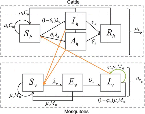
When an infectious mosquito bites a susceptible cow, there is a finite probability that the cow becomes infected. Since the duration of the latent period in cattle is small relative to their life span, we do not model the exposed stage. There is a substantial difference between the immune response of an infant and an adult cow. Young cows have a much higher probability of dying from RVF (10–70%) than adults (5–10%) 724. Similarly, 90–100% of goat and sheep infants die from RVF, while 10–30% of adults die from the virus 7. Since many adult cattle do not exhibit clinical signs apart from abortion of foetuses 121832, we include an asymptomatic class for infectious animals that transmit the virus at a lower rate than those with acute clinical signs. In our model, after successfully infected by an infectious mosquito, cattle move from the susceptible class S_h to either the infectious I_h or asymptomatic A_h class. After some time, the infectious and asymptomatic cattle recover and move to the recovered class, R_h. The recovered cattle have immunity to the disease for life. Cattle leave the population through a per capita natural death rate and through a per capita disease-induced death rate.

There is evidence that RVF is transmitted horizontally by livestock through contact with blood and aborted material 32. However, because it is not thought that this plays a role in long-term persistence of RVF, especially over a dry season, we do not include this mode of transmission in our model. If one were interested in predicting total consequence of a particular outbreak, the low levels of horizontal transmission may need to be included.

We divide the Aedes mosquito population into three classes: susceptible, S_v, exposed, E_v, and infectious, I_v. Female mosquitoes (we do not include male mosquitoes in our model because only female mosquitoes bite animals for blood meals) enter the susceptible class through birth. The birth term for mosquitoes accounts for and is proportional to the egg-laying rate of adult female mosquitoes; survival and hatching rate of eggs; and survival of larvae. If any of these are increased or decreased, the birth rate is affected accordingly. Since most density-dependent survival of mosquitoes occurs in the larval stage, we assume a constant emergence rate that is not affected by the number of eggs laid; that is, all emergence of new adult mosquitoes is limited by the availability of breeding sites.

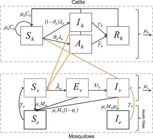
The virus enters a susceptible mosquito, S_v, with finite probability, when the mosquito bites an infectious animal and the mosquito moves from to the exposed class, E_v. After some period of time, depending on the ambient temperature and humidity 37, the mosquito moves from the exposed class to the infectious class, I_v. The mosquito remains infectious for life. Mosquitoes leave the population through a per capita natural death rate. We consider an additional model with susceptible, S_e, and infectious, I_e, juvenile classes to explore the effects of including an aquatic stage. This will facilitate a future inclusion of seasonality and mitigation strategies and allow us to compare our model with that of Adams and Boots’ 1 for dengue fever.

We ignore the feeding of mosquitoes on humans to keep the model simple and focus on livestock vector transmission. Although there is evidence that Aedes and Culex mosquitoes of the type typically spreading RVF have a preference for cattle and livestock as opposed to humans 28, we will include feeding on humans in the future because it is important to understand the effects of RVF morbidity in humans. Mpeshe et al. 26 present an RVF model that focuses on the human hosts. Also, although there is some evidence that mosquitoes preferentially feed on infected hosts 35, the evidence is sparse and we make the simplifying assumption that mosquitoes feed on all hosts equally.

Our adaptation of Chitnis et al.’s 910 and Gaff et al.’s 1617 models includes vertical transmission in mosquitoes with and without explicitly including the juvenile stage, generalizes the mosquito biting rate so that it applies to wider ranges of population sizes, and includes asymptomatic infections in cattle. In 16, the total number of mosquito bites on cattle depends on the number of mosquitoes, while in our model, the total number of bites varies with both the cattle and mosquito population sizes. This allows a more realistic modelling of situations where there is a high ratio of mosquitoes to cattle, and where cattle availability to mosquitoes is reduced through control interventions.

We compile two sets of baseline values for the parameters in the model: one for high rainfall and moderate temperature (wet season) and one for lower rainfall with moderate temperatures (dry season). The dry season parameter set can also be thought of as the result of mitigation strategies that reduce vector density, lifespan, and biting rate. Unusually high rainfall is often considered to be responsible for large RVF epidemics and in East Africa these events occur once every 3–7 years on average 2529. We also consider a range of values for vertical transmission of the virus from mosquito mother to egg of 1% to 10% 34. Vertical transmission is considered to be one of the main factors in inter-epidemic persistence of RVF 7192432 and has been included to various degrees in other RVF mathematical models 15–17. An alternative hypothesis for the inter-epidemic persistence of RVF is low-level endemic transmission with an unknown vertebrate host 19. Here, we explore only the vertical transmission hypothesis. We consider a range of parameter values for incubation time in the mosquito, as incubation also depends upon climate variability. For some parameters, we use values published in the available literature, while for others, we use realistically feasible values.

As ₀ is related to initial disease transmission, and ₀ is related to epidemicity, an evaluation of these sensitivity indices allows us to determine the relative importance of different parameters in RVF transmission and the likelihood and size of outbreaks. We analyse the relative importance of the parameters for three different purposes:

• the initial rate of disease transmission and epidemicity in areas of low rainfall;

• the initial rate of disease transmission and epidemicity in areas of high rainfall;

• the inter-epidemic persistence of disease with seasonal variation.

A knowledge of the relative importance of parameters can help guide in developing efficient intervention strategies in RVF-endemic or epidemic areas where resources are scarce.

2.1. Mathematical model

The state variables (Table 1) and parameters (Table 2) for the RVF model (Figure 1) satisfy the equations where μ_h is the per capita natural death rate for cattle. The total population sizes are and with and All parameters are strictly positive with the exception of the mosquito vertical transmission probability, ϕ_v, which is non-negative.

Table 1.  The state variables for the RVF model (1).

Sh	The number of susceptible cattle
Ah:	The number of asymptomatic cattle
Ih:	The number of infectious cattle
Rh:	The number of recovered cattle
Sv:	The number of susceptible Aedes mosquitoes
Ev:	The number of exposed Aedes mosquitoes
Iv:	The number of infectious Aedes mosquitoes
Nh:	Total cattle population
Nv:	Total Aedes mosquito population
Se:	The number of susceptible juvenile Aedes mosquitoes
Ie:	The number of infected juvenile Aedes mosquitoes
Ne:	Total Aedes juvenile population

Table 2. The parameters for the RVF model (1) and their dimensions.

μh	Per capita birth/death rate of cattle, Time^−1
μv	Per capita birth/death rate of Aedes mosquito species, Time^−1
ϕv	Probability of vertical transmission from an infectious Aedes mosquito mother to its eggs, dimensionless
θh	Probability of an infected cow moving to the asymptomatic stage. is the probability of an infected host moving to the infectious stage, dimensionless
σv	Number of times one mosquito would want to bite a cow per unit time, if cattle were freely available. This is a function of the mosquito's gonotrophic cycle (the amount of time a mosquito requires to produce eggs) and its preference for cattle blood, Time^−1
σh	The maximum number of mosquito bites a cow can sustain per unit time. This is a function of the cow's exposed surface area, the efforts it takes to prevent mosquito bites (such as switching its tail), and any vector control interventions in place to kill mosquitoes encountering cows or prevent bites, Time^−1
βhv	Probability of transmission of infection from an infectious mosquito to a susceptible cow given that a contact between the two occurs, dimensionless
βvh	Probability of transmission of infection from an infectious cow to a susceptible mosquito given that a contact between the two occurs, dimensionless
	Probability of transmission of infection from an asymptomatic cow to a susceptible mosquito given that a contact between the two occurs, dimensionless
νv	Per capita rate of progression of mosquitoes from the exposed state to the infectious state. 1/νv is the average duration of the latent period, Time^−1
γh	Per capita recovery rate for cattle from the infectious state to the recovered state. 1/γh is the average duration of the infectious period, Time^−1
	Per capita recovery rate for cattle from the asymptomatic state to the recovered state. is the average duration of the infectious asymptomatic period, Time^−1
δh	Per capita disease-induced death rate for cattle, Time^−1
C0	Stable cattle population in the absence of disease, animals
M0	Stable mosquito population, animals
γe	Per capita rate of progression from egg to adult, Time^−1

In this model, following the model of Chitnis et al. 9, σ_v is the rate at which a mosquito would like to bite a cow (related to the gonotrophic cycle length), and σ_h is the maximum number of bites that a cow can support per unit time (through physical availability and any intervention measures on livestock taken by humans). Then, σ_v N_v is the total number of bites that the mosquitoes would like to achieve per unit time and σ_h N_h is the availability of cattle. The total number of mosquito–cattle contacts is half the harmonic mean of σ_v N_v and σ_h N_h, In addition to having the correct limits at zero and infinity, this form also meets the necessary criteria that where b is the total number of bites per unit time. The total number of mosquito–cattle contacts depends on the populations of both species. We define as the number of bites per cattle per unit time, and as the number of bites per mosquito per unit time.

We define the force of infection from mosquitoes to cattle, , as the product of the number of mosquito bites that one cow has per unit time, b_h, the probability of disease transmission from the mosquito to the cow, β_hv, and the probability that the mosquito is infectious, I_v/N_v. We define the force of infection from cattle to mosquitoes, , as the force of infection from infectious (symptomatic and asymptomatic) cattle. This is defined as the number of cattle bites one mosquito has per unit time, b_v; the probability of disease transmission from an infected (asymptomatic) cow to the mosquito, β_vh (); and the probability that the cow is infectious, I_h/N_h (A_h/N_h).

The exposed class models the delay before infected mosquitoes become infectious. In mosquitoes, this delay is important because it is on the same order as their expected life span. Thus, many infected mosquitoes die before they become infectious.

To simplify the analysis of the model, we normalize the populations of each class of cattle and mosquitoes by their total species population size. We also assume that the mosquito population is at its stable equilibrium size, N_v=M₀. We let with Differentiating the scaling Equations (4) and solving for the derivatives of the scaled variables, we obtain and so on for the other variables. This creates a new six-dimensional system of equations,

The model (7) is epidemiologically and mathematically well-posed in the domain, This domain, D, is valid epidemiologically as the normalized populations, a_h, i_h, r_h, e_v, and i_v, are all non-negative and have sums over their species type that are less than or equal to 1. The cattle population, N_h, is positive and bounded by its stable disease-free value, C₀. We use the notation f′ to denote df/dt. We denote points in D by .

Theorem 2.1

Assuming that the initial conditions lie in , the system of equations for the RVF model (7) has a unique solution that exists and remains in for all time t≥0.

Proof

The right-hand side of Equation (7) is continuous with continuous partial derivatives in , so Equation (7) has a unique solution. We now show that is forward-invariant. We can see from Equation (7) that if a_h=0, then a_h′≥0; if i_h=0, then i_h′≥0; if r_h=0, then r_h′≥0; if e_v=0, then e_v′≥0; and if i_v=0, then i_v′≥0. It is also true that if then ; and if e_v+i_v=1 then e_v′+i_v′<0. Finally, we note that if N_h=0, then N_h′>0; if N_h>0 at time t=0, then N_h>0 for all t>0; and if N_h=C₀, then N_h′≤0. Therefore, none of the orbits can leave and a unique solution exists for all time.   ▪

2.2. Extended vertical transmission model

Here we extend the model by adding variables for the susceptible and the infected juvenile stages. Infected eggs and larvae result from vertical transmission of RVF from an infectious mother to her eggs. We can eventually relate the hatching of eggs to environmental variables and seasonality. Where there is little delay in hatching, we show the model reduces to the simpler vertical transmission model (1). We assume that the mosquito population is at a constant carrying capacity and that the birth term thus encompasses loss of eggs, regulation at the larval stage, and predation of eggs, larvae, or pupae. In most settings, this is a reasonable assumption as breeding sites are at carrying capacity. However, the assumption breaks down if the adult population drops substantially through, for example, vector control interventions. In the future, we will include seasonality and climate effects in the juvenile stage. We model the juvenile classes as either susceptible, S_e, or infected, I_e, that are replenished at a per capita birth rate μ_v. The proportion of eggs laid by an infected female mosquito that are infected is ϕ_v, while γ_e is the rate at which mosquitoes develop from egg to adult. The state variables (Table 1) and parameters (Table 2) for the RVF model (Figure 2) satisfy the equations

Figure 2. Susceptible cattle, S_h, can be infected when they are bitten by infectious mosquitoes. Infected cattle either become infectious and sick, I_h, or asymptomatic carriers A_h (with a lower infectivity to mosquitoes). They then recover with a constant per capita recovery rate to enter the recovered, R_h, class. Susceptible mosquitoes, S_v, can become infected when they bite infectious cattle. The infected mosquitoes then move through the exposed, E_v, and infectious, I_v, classes. Birth and death of the population are shown in the figure as well. The aquatic stage of mosquitoes is included explicitly, where some eggs laid by infectious mosquitoes, I_v, are infected, I_e, and all other eggs are susceptible, S_e.

To simplify the analysis of the model, we normalize the populations of each class of cattle and mosquitoes by their total species population size. We also assume that the mosquito population is at its stable equilibrium size, N_v=M₀ and . We normalize the variables by their respective population size,

with Differentiating the scaling equations (10) and solving for the derivatives of the scaled variables as before, we obtain a new seven-dimensional system of equations,

The model (12) is epidemiologically and mathematically well-posed in the domain, This domain, ₂, is valid epidemiologically as the normalized populations, a_h, i_h, r_h, i_e, e_v, and i_v, are all non-negative and have sums over their species type that are less than or equal to 1. The cattle population, N_h, is positive and bounded by its stable disease-free value, C₀. We use the notation f′ to denote df/dt. We denote points in ₂ by .

Theorem 2.2

Assuming that the initial conditions lie in ₂, the system of equations for the RVF model (12) has a unique solution that exists and remains in ₂ for all time t≥0.

Proof

The right-hand side of Equation (12) is continuous with continuous partial derivatives in ₂, so Equation (12) has a unique solution. We now show that ₂ is forward-invariant. We can see from Equation (12) that if a_h=0, then a_h′≥0; if i_h=0, then i_h′≥0; if r_h=0, then r_h′≥0; if i_e=0, then i_e′≥0; if e_v=0, then e_v′≥0; and if i_v=0, then i_v′≥0. It is also true that if then ; if i_e=1, then i_e′<0; and if e_v+i_v=1, then e_v′+i_v′<0. Finally, we note that if N_h=0, then N_h′>0; if N_h>0 at time t=0, then N_h>0 for all t>0; and if N_h=C₀, then N_h′≤0. Therefore, none of the orbits can leave ₂ and a unique solution exists for all time.   ▪

3. Equilibrium points and basic reproductive number

3.1. Disease-free equilibrium point

Disease-free equilibrium points are steady-state solutions where there is no disease. We define the ‘diseased’ classes as the cattle or mosquito populations that are either asymptomatic, exposed, or infectious; that is, a_h, i_h, e_v, and i_v for model (7). We denote the positive orthant in ℝⁿ by and the boundary of by .

Theorem 3.1

The model for RVF without a juvenile class (7) has exactly one equilibrium point, with no disease in the population (on .

Proof

By inserting x_dfe in Equation (7), we see that all derivatives are equal to zero so x_dfe is an equilibrium point of Equation (7). By setting any of a_h, i_h, r_h, e_v, or i_v equal to zero, we also see that the other four variables have to be zero and N_h=C₀ for the system to be at equilibrium.   ▪

3.1.1. Extended model disease-free equilibrium

We define the ‘diseased’ classes as the cattle or mosquito populations that are either asymptomatic, exposed, or infectious; that is, a_h, i_h, i_e, e_v, and i_v for model (12).

Theorem 3.2

The model for RVF without a juvenile class (12) has exactly one equilibrium point, with no disease in the population (on .

Proof

By inserting x_dfe, 2 in Equation (12), we see that all derivatives are equal to zero so x_{dfe, 2} is an equilibrium point of Equation (12). By setting any of a_h, i_h, r_h, i_e, e_v, or i_v equal to zero, we also see that the other five variables have to be zero and N_h=C₀ for the system to be at equilibrium.   ▪

3.2. Basic reproduction number and reactivity

In a model assuming a homogeneous population and with one infectious compartment, the basic reproductive number, ₀, is defined as the expected number of secondary infections that one infectious individual would cause over the duration of the infectious period in a fully susceptible population. For our more complicated models, we use the next generation operator approach, as described by Diekmann et al. 14 and Van den Driessche and Watmough 40 to define the basic reproductive number, ₀, to describe a threshold condition for when the disease-free equilibrium points lose stability. For the model without juvenile stages, Equation (1), we let and , where represents the rate of new infections entering the population, and represents the rate of movement (by other means) out of, and into, each compartment, respectively. We let F₀ and V₀ be the Jacobian matrices of the first four elements of and , respectively, evaluated at the disease-free equilibrium, x_dfe. Then, and where The basic reproductive number is the spectral radius of the next generation matrix, , where s(A) denotes the absolute value of the largest eigenvalue of A and where

Theorem 3.3

The disease-free equilibrium point, x_dfe of the model for RVF without juvenile stages (7), is locally asymptotically stable when and unstable when .

Proof

, , and satisfy assumptions (A1)–(A5) in 40 so this theorem is a straightforward application of Theorem 2 in 40.   ▪

When there is no vertical transmission, ϕ_v=0, ₀ resembles the basic reproductive number for malaria [(3.4)]9. In that case, it is geometric mean of the number of new infections in livestock from one infected mosquito, R_hv, and the number of new infections in mosquitoes from one infected cow, R_vh, in the limiting case that both populations are fully susceptible. The number of new infections in cows from a newly infected mosquito, R_hv, is the product of the probability that the mosquito survives the exposed stage (), the number of bites on cows per mosquito (ζ C₀), the probability of transmission per bite (β_hv), and the infectious life span of a mosquito (1/μ_v) 22. The number of new infections in mosquitoes from one cow, R_vh, is the weighted sum of new infections resulting from asymptomatic and infectious cows. This is the product of the number of bites one cow receives (ζ M₀), the probability of transmission per bite ( for an asymptomatic cow and β_vh for an infectious cow), and the duration of the infective period ( for an asymptomatic cow and for an infectious cow) weighted by the probability that a cow either becomes asymptomatic or infectious upon infection. In the presence of vertical transmission, ϕ_v>0, ₀ increases because vertical transmission directly increases the number of infectious mosquitoes and indirectly increases the transmission from cows to mosquitoes and back to cows. We keep with the notation of the next generation operator methods 40 so the square root denotes the number of new infections from one infected cow to mosquitoes, or vice versa. ₀ then determines whether or not it is possible for RVF to be endemic in the population being considered.

RVF is characterized by large outbreaks and periods of relative senescence so we also consider the reactivity (epidemicity) of the model, or the potential for the system to support transitory epidemics. Reactivity can be thought of as the maximum instantaneous amplification rate of the state variables from equilibrium following a perturbation 21. The system is reactive when the amplification rate is positive, and not reactive when it is non-positive. For our case, reactivity is the spectral radius of the Hermitian part of the Jacobian for the system of the unscaled variables (1) evaluated at the disease-free equilibrium, , where is the Hermitian part of the matrix A 31.

Hosack et al. 21 derive a reactivity threshold, , for the reactivity of a vector–host susceptible-infectious-recovered-type model. Near the disease-free equilibrium, for the system (1), (where Fˆ₀ and Vˆ₀ are defined in a similar manner to F₀ and V₀ except that they are evaluated for the unscaled model (1) instead of the scaled model (7)). If then the system is reactive and an epidemic can result from a perturbation of the disease-free state. When considering the prevalence of infected individuals, one can think of the reactivity index ₀ as being the maximum number of secondary infections that could result from introducing one infectious individual into a fully susceptible population. For RVF, the most likely perturbation resulting in a transitory epidemic is the emergence of large numbers of adult mosquitoes, some of which are infected from birth via vertical transmission. As mentioned earlier, the general model (1) with its associated parameter values satisfies the assumption required for the analysis in 40 as well as in 21, including the condition that H(Fˆ₀) be non-negative and H(Vˆ₀) be non-singular with non-negative inverse. H(Vˆ₀) has a non-negative inverse when . For Equation (1), ₀ does not have an easily interpreted analytic expression, so we compute it numerically for the baseline parameter values.

3.2.1. Extended model basic reproduction number and reactivity

We use the same methods to compute the basic reproductive number and reactivity threshold for the extended model (12). Let and , where represents the rate of new infections entering the population, and represents the rate of movement (by other means) out of, and into, each compartment, respectively. We let F_{0, 2} and V_{0, 2} be the Jacobian matrices of the first five elements of ₂ and ₂, respectively, evaluated at the disease-free equilibrium, x_{dfe, 2}. Then, for the model with an explicit juvenile stage (12), and The basic reproductive number is the spectral radius of the next generation matrix, ,

Theorem 3.4

The disease-free equilibrium point, x_{dfe, 2} of the model for RVF with explicit juvenile stages (12), is locally asymptotically stable when and unstable when .

Proof

, , and satisfy assumptions (A1)–(A5) in 40 so this theorem is a straightforward application of Theorem 2 in 40.   ▪

We note that , so explicitly including the juvenile stages in a manner similar to that used in 1 does not change the value of the basic reproductive number.

The reactivity threshold of the unscaled model (9) around the disease-free equilibrium for the extended model is (where Fˆ_{0, 2} and Vˆ_{0, 2} are defined in a similar manner to F_{0, 2} and V_{0, 2} except that they are evaluated for the unscaled model (9) instead of the scaled model (12)). Unlike the basic reproductive number, the reactivity index for the model with juvenile stages (9) is different from that of the original model (1). The effect of the larval stage cancels out for ₀ but remains a factor in the Hermitian parts of the next generation matrices and the Jacobian. It is important to note here that for some parameter values the condition that H(Vˆ₀) have a non-negative inverse is not met. The condition is met when and when . If it is not met, then we must instead use the original definition of reactivity , where J_{0, 2} is the Jacobian of the unscaled RVF model with juvenile stages (9) evaluated at the disease-free equilibrium x_{dfe, 2}, to determine whether our system is reactive.

3.3. Endemic equilibrium points

Endemic equilibrium points are steady-state solutions where disease persists in the population. While it is possible to explicitly solve for the endemic equilibrium point using symbolic software package such as Mathematica, the results are too complex to extract insight from. We therefore use a theorem by Rabinowitz 33 in a similar manner to that used in 9 to show the existence of an endemic equilibrium for all values of R₀>1.

We first rewrite the equilibrium equations of Equation (7) for as a nonlinear eigenvalue problem in a Banach space, where , with Euclidean norm, |·|; (Equation (18)) is the bifurcation parameter; L is a compact linear map on ℝ³; and h(ζ, u) is uniformly on bounded ζ intervals. We also define so that the pair .

A theorem by Rabinowitz [Theorem 1.3]33 states that if ζ₀ is a characteristic value (reciprocal of a real non-zero eigenvalue) of L of odd multiplicity, then there exists a continuum of non-trivial solution pairs, (ζ, u) of Equation (26) that intersects the trivial solution (i.e. (ζ, 0) for any ζ) at (ζ₀, 0) and either meets infinity in Ω (is unbounded) or meets where is also a characteristic value of L of odd multiplicity. We use this theorem to show that such a continuum of solution pairs exists for the eigenvalue equation (26) that meets infinity in Ω. We then show that to each of these solution pairs, there corresponds an equilibrium pair . We define the equilibrium pair, , as the collection of a parameter value, ζ, and the corresponding equilibrium point, x_ee, for that parameter value, of the RVF model (7). We finally show that the range of ζ where this equilibrium pair exists corresponds to R₀>1.

For the rest of this subsection, we use the variables, a_h, i_h, r_h, N_h, e_v, and i_v to represent the equilibrium values of the state variables and not the values at any time t. We replace σ_h and σ_v with ζ and to rewrite the equilibrium equations as We solve Equations (27a), (27d), and (27f) for N_h, r_h, and i_v in terms of a_h, i_h, and e_v, Substituting Equation (28) in, and taking the Taylor polynomial expansions of, the left-hand sides of Equations (27b), (27c), and (27e) with respect to a_h, i_h, and e_v around (0, 0, 0), we can rewrite Equations (27b), (27c), and (27e) in the form of Equation (26) with The matrix L has three eigenvalues: , 0, and, . Therefore, the two characteristic values of L are The right eigenvectors corresponding to ξ₁ and ξ₂ are and respectively.

From Theorem 1.3 of Rabinowitz 33, we know that there is a continuum of solution pairs , whose closure contains the point (ξ₁, 0), that either meets infinity (is unbounded) or the point (ξ₂, 0). We denote the closure of a set by and denote the continuum of solution pairs emanating from (ξ₁, 0) by , where ; and from (ξ₂, 0) by , where . We introduce the sets

Lemma 3.5

The initial direction of the branch of equilibrium points, near the bifurcation point (ξ₁, 0) (or (ξ₂, 0)), is equal to the right eigenvector of L corresponding to the characteristic value ξ₁ (or ξ₂).

Proof

We use Lyapunov–Schmidt expansion, as described by Cushing 11, to determine the initial direction of the continua of solution pairs, and . We expand the terms of the nonlinear eigenvalue equation (26) about the bifurcation point, (ξ₁, 0). The expanded variables are Evaluating the substitution of the expansions (32) into the eigenvalue equation (26) at we obtain . This implies that u⁽¹⁾ is the right eigenvector of L corresponding to the eigenvalue 1/ξ₁, v₁. Thus, close to the bifurcation point, the equilibrium point can be approximated by , , and .

A similar expansion around the bifurcation point (ξ₂, 0) would show that the initial direction of the branch of equilibrium points in the direction of the right eigenvector L corresponding to the eigenvalue 1/ξ₂.   ▪

Lemma 3.6

For all u∈U₁, a_h>0, i_h>0, and e_v>0.

Proof

By Theorem 3.1, there are no equilibrium points on other than , so . We know from Lemma 3.5 that close to the bifurcation point, (ξ₁, 0), the direction of U₁ is equal to v₁, the right eigenvector corresponding to the characteristic value, ξ₁. As v₁ contains only positive terms, U₁ is entirely contained in . Thus, for all u∈U₁, a_h>0, i_h>0, and e_v>0.   ▪

Lemma 3.7

The point corresponds to (on ). For every solution pair there corresponds one equilibrium pair where x* is in the positive orthant of ℝ⁶.

Proof

We first show that u=0 corresponds to x_dfe. As , by Theorem 3.1 we know that the only possible equilibrium point is x_dfe. We now show that for every ζ∈Z₁ there exists an x* in the positive orthant of ℝ⁶ for the corresponding u∈U₁. By Lemma 3.6, we know that a_h>0, i_h>0, and e_v>0. From Equation (28), we see that for every positive a_h, i_h, and e_v, there exist corresponding positive r_h, N_h, and i_v.   ▪

Lemma 3.8

The set Z₁ is unbounded.

Proof

As shown in Lemma 3.6, and U₁ is entirely contained in . We can similarly show that U₂ is entirely outside of because v₂ contains negative terms.

Therefore, and do not intersect and by Theorem 1.3 of Rabinowitz 33, meets infinity. From Theorem 2.1, we know that the equilibrium points are bounded so U₁ does not meet infinity. Therefore, Z₁ must be unbounded.   ▪

Theorem 3.9

The transcritical bifurcation point at ζ=ξ₁ corresponds to and there exists at least one endemic equilibrium point of the RVF model (7) for all .

Proof

From Lemmas 3.7 and 3.8, we know that there exists a continuum of equilibrium pairs that exists for all values of ζ>ξ₁.

Some algebraic manipulations after substituting ζ=ξ₁ (Equation (30a)) into the definition of ₀ (Equation (20)) lead to . For any , Equation (20) defines a corresponding ζ>ξ₁, and therefore there exists a corresponding equilibrium point. It is possible, though not necessary, for the continuum of equilibrium pairs to include values of ζ<ξ₁ ().   ▪

Thus, when , the model (7) is guaranteed to have at least one endemic equilibrium point. Although we do not show its stability, we conjecture that this endemic equilibrium point is locally asymptotically stable for .

3.3.1. Extended model endemic equilibrium points

For the RVF model with juvenile stages, we can show the existence of at least one endemic equilibrium point for all values of in a similar manner to that for the model without juvenile stages. Compared to Equation (7), for Equation (12), the equilibrium point is in ℝ⁷ instead of ℝ⁶, there is an additional equilibrium equation, and the equilibrium equation (27f) is replaced by

Theorem 3.10

The transcritical bifurcation point at ζ=ξ₁ corresponds to and there exists at least one endemic equilibrium point of the RVF model with juvenile stages (12) for all .

Proof

Solving Equation (33a) for i_e provides . Substituting i_e in Equation (33b) provides as in Equation (28b). The rest of the proof follows as for the proof of Theorem 3.9 with the endemic equilibrium in ℝ⁷.   ▪

Again, while we do not show the stability of the endemic equilibrium point for the RVF model with juvenile stages, we conjecture that it is locally asymptotically stable for .

4. Sensitivity analysis

In determining how best to reduce cattle mortality and morbidity due to RVF, it is necessary to know the relative importance of the different factors responsible for its transmission and prevalence. Initial disease transmission and endemicity is directly related to ₀ and the potential size of outbreaks is directly related to ₀. We calculate the sensitivity indices of the reproductive number ₀ and the reactivity index ₀ to the parameters in the model at baseline values described in Tables 3 and 4. These indices tell us how crucial each parameter is to disease transmission, epidemicity, and prevalence. Sensitivity analysis is commonly used to determine the robustness of model predictions to parameter values. Here we use it to discover parameters that have a high impact on ₀ and ₀ and should be targeted by intervention strategies.

Table 3. The parameters for the RVF model for high rainfall and moderate temperatures (wet season) for Equation (1) with values, range, and references.

Parameter	Baseline	Range	Reference
1/μh	2190	1825–2555	1630
1/μv	20	10–30	131624
ϕv	0.1	0–1	34
θh	0.4	0.3–0.6	732
σv	0.33	0.1–0.5	510
σh	19	0.1–50	10
βhv	0.21	0.001–0.54	233237
βvh	0.7	0.3–0.9	2332,37–39
	0.3	0.1–0.5	1032
1/νv	14	7–20	52337
1/γh	4	1–7	571724
	4	1–7	724
δh	0.10	0.05–0.30	724
γe	0.20	0.1–0.3
M0	20,000	15,000–25,000	17
C0	1000	500–2000	17

Note: Time is in days.

Table 4. The parameters for the RVF model for low moisture and moderate temperatures (dry season or wet season with mitigation) for Equation (1) with values, range, and references.

Parameter	Baseline	Range	Reference
1/μh	2190	1825–2555	1730
1/μv	14	7–20	1324
ϕv	0.1	0–1	34
θh	0.4	0.3–0.6	732
σv	0.25	0.1–0.5	510
σh	19	0.1–50	10
βhv	0.21	0.001–0.54	233237
βvh	0.7	0.3–0.9	2332,37–39
	0.3	0.1–0.5	1032
1/νv	14	7–20	52337
1/γh	4	1–7	5724
	4	1–7	724
δh	0.10	0.05–0.30	724
γe	0.10	0.05–0.2
M0	4000	3000–5000	17
C0	1000	500–2000	17

Note: Time is in days.

4.1. Description of sensitivity analysis

Local sensitivity indices allow us to measure the relative change in a state variable when a parameter changes. In computing the sensitivity analysis, we use methods described by Arriola 4. The normalized forward sensitivity index of a variable to a parameter is the ratio of the relative change in the variable to the relative change in the parameter. When the variable is a differentiable function of the parameter, the sensitivity index may be alternatively defined using partial derivatives.

Definition 4.1

The normalized forward sensitivity index of a variable, u, that depends differentiably on a parameter, p, is defined as

There is a detailed example of evaluating these sensitivity indices in 10.

4.2. Sensitivity indices of ₀

Since we have an explicit formula for ₀, we compute the sensitivity indices analytically at the baseline parameter values. ₀ is the same for the models with and without juvenile stages, hence the sensitivity indices are the same for both models. The indices , or the local sensitivity of ₀ to a parameter p, are recorded in Table 5 for both the dry season and wet season. A simulation for an epidemic with wet season parameters and with , with a fully susceptible host population and one infectious mosquito are shown in Figure 3. A similar simulation with dry season parameters with is shown in Figure 4.

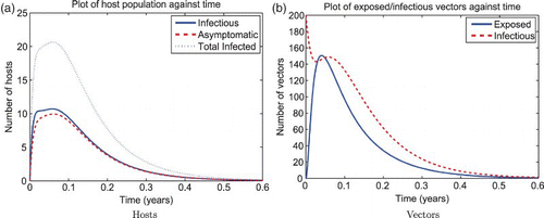
Figure 3. Solution of the RVF model (1) for the wet season parameters with

₀=2.28. The initial conditions are S_h=1000, A_h=I_h=R_h=0, S_v=19999, E_v=0, and I_v=1. The y-axis is on a log scale since the initial epizootic is much larger than subsequent outbreaks. (a) Hosts and (b) vectors.

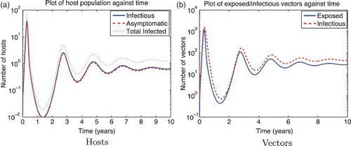
Figure 4. Solution of the RVF model (1) for the dry season (or mitigated wet season) parameters with

₀=0.80. The initial conditions are S_h=1000, A_h=I_h=R_h=0, S_v=3999, E_v=0, and I_v=1. (a) Hosts and (b) vectors.

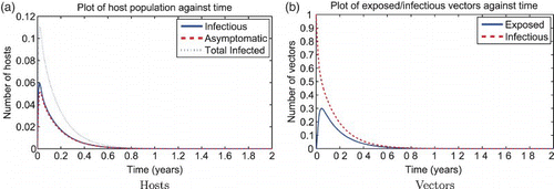
Table 5. Sensitivity indices of ₀ (Equation (20)) to parameters for the RVF model, evaluated at the baseline parameter values given in Tables 3 and 4.

	Dry season		Wet season
	Parameter	Sensitivity index	Parameter	Sensitivity index
1.	σv	+0.89	σv	+0.73
2.	μv	−0.70	μv	−0.69
3.	βhv	+0.47	βhv	+0.49
4.	C0	−0.42	βvh	+0.35
5.	M0	+0.42	σh	+0.25
6.	βvh	+0.33	γh	−0.25
7.	γh	−0.24	C0	−0.24
8.	νv	+0.23	M0	+0.24
9.		+0.13	νv	+0.20
10.		−0.13		+0.14
11.	δh	−0.095		−0.14
12.	θh	−0.089	δh	−0.10
13.	ϕv	+0.067	θh	−0.09
14.	σh	−0.047	ϕv	+0.022
15.	μh	−0.0007	μh	−0.0007

Notes: The parameters are ordered from most sensitive to least. For both wet and dry seasons, the most sensitive parameter is the mosquito biting rate, σ_v, and the least sensitive parameter is the cow death rate, μ_h. A negative sensitivity index indicates if the parameter increases, ₀ decreases, while a positive sensitivity index means that ₀ increases as the parameter increases.

For both seasons, ₀ is most sensitive to the mosquito biting rate σ_v, so decreasing the mosquito biting rate by 10% would decrease ₀ by 7.3% for the dry season and 8.9% for the wet season. ₀ is also sensitive to the mosquito birth/death rate μ_v and the transmission rate from infected mosquito to cow β_hv for both seasons. If μ_v increases by 10% (so the lifespan of mosquitoes is decreased), then ₀ decreases by about 7% and if β_hv increases by 10% then ₀ increases by about 4.7% for both wet and dry seasons (however, it would be difficult to decrease β_hv in the field). Also, note that . This is because the vector-to-host ratio is important in the initial spread of RVF for the parameter space being considered. Therefore, increasing the number of hosts while leaving the number of mosquitoes constant would decrease ₀, while increasing the number of vectors and leaving the number of hosts constant would increase ₀.

After the first three most sensitive parameters, the wet season and dry season sensitivity indices diverge. For the wet season, the next three parameters to which ₀ is most sensitive are the transmission from infected cow to mosquito β_vh, the number of bites a host can sustain σ_h, and the rate of recovery for infectious cows γ_h. The dry season is sensitive next to the carrying capacities of the mosquitoes and cows, M₀ and C₀, respectively, and to transmission from infected cow to mosquito β_vh. So we see that during the dry season when the number of mosquitoes is low, ₀ depends more on the vector-to-host ratio via M₀ and C₀. If C₀ is increased by 10% then ₀ decreases by 4.2% and if M₀ is decreased by 10% then ₀ will decrease by 4.2%. Finally, ₀ is not particularly sensitive to the vertical transmission rate ϕ_v, although it is more important in the dry season with mosquito populations low. This indicates that as control measures for ₀ drive ₀ lower, vertical transmission may become more important.

4.3. Sensitivity indices of ₀

The reactivity index of the unscaled RVF model without juvenile stages in the wet season is . We show a simulation of the unscaled RVF model (1) for wet season parameters in Figure 5 with the effects of the changing population size through disease-induced mortality. Normally, the herd immunity is reached when the proportion of immune are above . However, in this simulation, pathogen transmission continues to occur at immune proportion values greater than though still less than . Though less so than the wet season, the dry season is also reactive, , so given a strong enough perturbation an epidemic can still occur as shown in Figure 6.

Figure 5. Solution of the RVF model (1) for the wet season parameters with

₀=2.28 where the magenta line is total cattle and the green line is recovered cattle. The blue dashed line is N_h(1−1/

₀), the purple dotted line is N_h(1−1/

₀), and the aqua dotted line is . The initial conditions are S_h=1000, A_h=I_h=R_h=0, S_v=19999, E_v=0, and I_v=1.

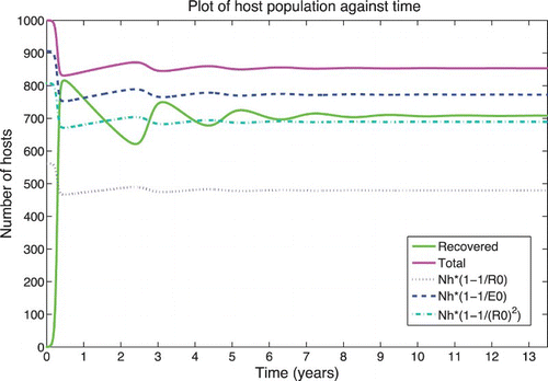
Figure 6. Solution of the RVF model (1) for the dry season parameters with initial conditions perturbed to wet season mosquito population levels and hatching infectious eggs. The initial conditions are S_h=1000, A_h=I_h=R_h=0, S_v=19999, E_v=0, and I_v=200. The final number of cows infected is 300. (a) Hosts and (b) vectors.

We summarize the numerical estimation of these indices in Table 6. The top five parameters to which ₀ is most sensitive are the same for both the wet season and the dry season, although the order changes between seasons. ₀ is most sensitive to the mosquito biting rate σ_v, the mosquito and cow carrying capacities M₀ and C₀, the transmission rate from infectious cow to mosquito β_vh, and the death rate of mosquitoes μ_v. If σ_v increases by 10% then ₀ increases by 9.4% for wet and 7.4% for dry season; if β_vh increases by 10% then ₀ increases by 7.9% for wet and 7.6% for dry season; if C₀ decreases by 10% or if M₀ increases by 10% then ₀ increases by 7.3% for wet and 9.1% for dry season.

Table 6. Sensitivity indices of ₀ to parameters for the RVF model (1), evaluated at the baseline parameter values given in Tables 3 and 4.

	Dry season		Wet season
	Parameter	Sensitivity index	Parameter	Sensitivity index
1.	σv	+0.94	βvh	+0.79
2.	C0	−0.91	σv	+0.74
3.	M0	+0.91	C0	−0.73
4.	βvh	+0.76	M0	+0.73
5.	μv	−0.39	μv	−0.40
6.	γh	−0.28	γh	−0.28
7.		+0.20	σh	+0.26
8.	δh	−0.11		+0.20
9.	νv	−0.11	δh	−0.11
10.		−0.10		−0.10
11.	σh	+0.050	νv	−0.10
12.	βhv	+0.030	βhv	+0.0074
13.	ϕv	+0.059	θh	−0.0014
14.	θh	−0.056	ϕv	+0.0014
15.	μh	−0.0007	μh	−0.0007

Notes: The parameters are ordered from most sensitive to least. For both wet and dry seasons, the least sensitive parameter is the cow death rate, μ_h.

Initial disease transmission ₀ and epidemicity (or reactivity) ₀ are more sensitive to different parameters, so control efforts must consider this. Different parameters will have more effect on endemicity and initial disease transmission than on the probability of a transient epidemic given a perturbation. For example, both ₀ and ₀ are sensitive to the mosquito biting rate σ_v and the mosquito death rate μ_v for both seasons. However, changes in the vector-to-host ratio via the host and vector carrying capacities C₀ and M₀ will have a large effect on ₀ in the wet season while not much of an effect on ₀. ₀ is also highly sensitive to β_vh for both wet and dry seasons, while ₀ is much less sensitive to the transmission from host to vector. It is possible for ₀ to be low while reactivity is high, so that a large transient epidemic can occur (Figure 6). Therefore, controlling ₀ may be important even when the basic reproductive ratio is below 1.

4.4. Sensitivity of reactivity for the Juvenile model

For the model with juvenile stages with wet season parameter values, we cannot use the reactivity index _{0, 2} since conditions for existence are not met for perturbations of wet season parameters, so instead we will consider sensitivity of the reactivity rate, , to the parameters. For the wet season, the reactivity rate is most sensitive (in order of importance) to the transmission rate from host to vector, β_vh; the biting rate of the mosquitoes, σ_v; the host and vector carrying capacities, C₀ and M₀; the number of bites a host can sustain, σ_h; and the transmission from asymptomatic hosts to the vector, . The dry season parameter values allow sensitivity analysis of the reactivity index, _{0, 2}. The reactivity index is most sensitive (in order of importance) to the vector biting rate σ_v; the host and vector carrying capacities, C₀ and M₀; the transmission rate from host to vector, β_vh; the recovery rate of hosts, γ_h; and the transmission rate from asymptomatic host to vector, .

As with the original model, reactivity is insensitive to vertical transmission; however, it is more sensitive to vertical transmission for the dry season parameter set than for the wet season parameters. The extended model is also not sensitive at all to the larvae hatching rate during the wet season; it is slightly more sensitive to the hatching rate during the dry season. The sensitivity indices are summarized in Table 7. In conclusion, the extended juvenile model for our parameter space is sensitive to the same major parameters that the original model is sensitive to.

Table 7. Sensitivity indices of _{0, 2} for the dry season and ˜_{0, 2} for the wet season to parameters for the RVF model with juvenile stages (9), evaluated at the baseline parameter values given in Tables 3 and 4.

	Dry season (0, 2)		Wet season ()
	Parameter	Sensitivity index	Parameter	Sensitivity index
1.	σv	+0.94	βvh	+0.95
2.	C0	−0.90	σv	+0.84
3.	M0	+0.90	C0	−0.84
4.	βvh	+0.75	M0	+0.84
5.	μv	−0.57	σh	+0.29
6.	γh	−0.28		+0.18
7.		+0.20	γh	−0.06
8.	δh	−0.11	δh	−0.02
9.		−0.10	νv	−0.02
10.	γe	+0.09	μv	−0.02
11.	σh	+0.05		−0.01
12.	βhv	+0.04	βhv	−0.0003
13.	νv	−0.02	θh	−0.0001
14.	θh	−0.008	μh	−0.0001
15.	ϕv	+0.007	γe	0
16.	μh	−0.0007	ϕv	0

Note: The parameters are ordered from most sensitive to least.

4.5. Global sensitivity analysis

In addition to the local sensitivity analysis, we performed global sensitivity analysis on ₀ and ₀, showing the effects of variance in ₀ and ₀ due to each parameter alone, as well as the influence of higher order effects. For the global analysis, we varied the parameters along the entire dry season and wet season range. We also varied the vertical transmission rate from 0 to 1 since the actual vertical transmission rate is not known. The global analysis confirms the local sensitivity results. Across the whole range, ₀ is most sensitive to the transmission probability from vector to host, vector death rate, vector biting rate, host recovery rate, carrying capacity of vectors, and the number of bites a host can sustain. Sensitivity to each of these parameters varies depending on whether we are considering the wet or dry season parameters. Vertical transmission can be important to ₀ if it ranges from 0 to 1. Across the whole range, ₀ is most sensitive to host and vector carrying capacities, the vector death and biting rates, the probability of transmission from host to vector, and the number of bites a host can sustain. Global sensitivity analysis also indicates that higher order effects can be important. The effect of changing β_hv on ₀ can vary depending on the values of the other parameters. This is especially true for the dry season parameter range, implying that for future studies a closer analysis of higher order interactions may be useful.

5. Numerical results with seasonality

We consider the introduction of RVF in a naive population in order to understand how it persists as it expands into new regions and to understand the history of its expansion over the past decades. The low-level endemic equilibrium for the wet/high season parameters is only reached after the disease effectively dies out following the first large epidemic (Figure 3). This is due to the high level of herd immunity reached in the hosts after the first epidemic in which many are infected. So in reality, even with wet season conditions all year, an endemic equilibrium would not be reached without some mode of inter-epidemic persistence such as long-lasting infected eggs or an introduced infected host. This suggests that seasonality combined with mosquito vertical transmission and/or introduction of new infected individuals after immunity wanes is necessary for the survival of RVF. Without these mechanisms, it is likely to die out within a year or two.

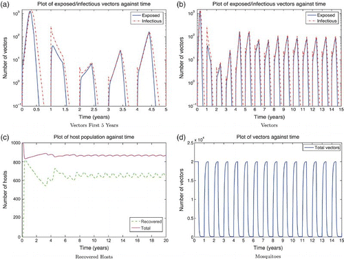
In order to explore inter-epidemic persistence, we consider a simple seasonal version of the model. To implement seasons, we run the simulations for the wet season for 182 days and the dry season for 183.25 days. Every wet season is followed by a dry season. Compartments with less than one individual at the end of a season are set equal to zero. The simulation is run for 20 years. We assume that the eggs Aedes mosquitoes lay during the last 4 weeks of the wet season will overwinter and about ⅔ of them will survive and hatch in the next wet season 15. Under these assumptions, RVF persists and eventually settles to endemic yearly cycles (Figure 7). However, under our assumptions, inter-epidemic persistence is very sensitive to the probability of vertical transmission: when , RVF dies out, and when , the disease persists on the scale we consider. Alternatively, if an infected host were to be introduced at the opportune time, RVF could reach the endemic yearly cycles observed in the simulations (Figure 7). Since both vertical transmission and the introduction of infected hosts at the right time are relatively rare events, we expect that both play a role in the persistence of RVF. Our simulations suggest that even low rates of vertical transmission can contribute significantly to inter-epidemic persistence. We do not include eggs that hatch several years after laid, an aspect of the system that could decrease the level of vertical transmission needed for persistence.

Figure 7. Solution of the RVF model (9) with seasonality, setting infected populations below 1 at the end of each season to 0. It is assumed the last 4 weeks of wet season adults contribute to the eggs that will hatch in the following wet season with a dry season survival rate of 2/3. Wet season parameters are used for 4 months, followed by dry season parameters with vector carrying capacity M₀=100. The y-axis of subfigures (a) and (b) are on a log scale. Subfigure (a) show a large epizootic in the first year followed by many infectious mosquitoes hatching in year 2, and negligible infection in year 3 due to high levels of herd immunity. The exposed and infectious mosquito trajectories stabilize to yearly outbreaks after the first 5 or 6 years (subfigure (b)). (a) Vectors first 5 years; (b) vectors; (c) recovered hosts; and (d) mosquitoes.

Next, we vary the rainfall via different mosquito wet season carrying capacities (M₀). As expected, more sporadic epidemics occur that look qualitatively similar to what is observed in the field (Figure 8). For varying rainfall, vertical transmission rates must be higher for persistence than with regular rainfall: for RVF dies out, while for , it persists over the 20 years of the simulation. Again, vertical transmission with egg survival can explain persistence over the time frame of several years, but seems unlikely to account for decades-long persistence in a closed system. We would guess that low-level transmission in an alternate host or the introduction of infected individuals from outside the system would work along with vertical transmission to explain persistence of RVF.

Figure 8. Solution of the RVF model (9) with seasonality and varying rainfall via changing wet season mosquito carrying capacity, setting infected populations below one at the end of each season to zero. It is assumed the last four weeks of wet season adults contribute to the eggs that will hatch in the following wet season with a dry season survival rate of ⅔. Subfigure (a) shows the first 6 years of epizootics on a log scale. Herd immunity, rainfall (via mosquito carrying capacity), and hatched infectious eggs from the previous year affect the timing and magnitude of outbreaks. Subfigure (b) shows infectious mosquitoes over a 19 year period. (a) Hosts; (b) Vectors; (c) Recovered Hosts; (d) Mosquitoes.

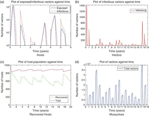
For varied rainfall, we observe that particularly high rainfall (as in year 3) does not always result in an outbreak. However, the following year, which had normal wet season rainfall, saw a large epidemic. This hints at the importance of host–vector dynamics in addition to weather in explaining RVF outbreaks. Although unusually high rainfall is a good predictor for Kenya and East Africa, epidemics in West and South Africa do not always coincide well with abnormal weather events. This confirms the need for models that include disease, host, and vector dynamics in addition to weather data.

5.1. Juvenile model

Numerical simulations of the juvenile class extension produce results quite similar to the original model with parameters describing the wet season alone or the dry season alone. Although the basic reproductive number, ₀, is the same for both the original and juvenile model, the reactivity index is slightly larger for the juvenile case than the original model, .

For the seasonal case, if we reduce the hatching rate to zero during the dry season so that infectious eggs from the end of the wet season are stored, the results are similar to those of the original model with seasonality. As before, a threshold of vertical transmission probability of 0.015 is needed for persistence. For varying annual levels of rainfall, higher levels of vertical transmission are needed for persistence (vertical transmission probability of about 0.03). Figure 9 shows the infected eggs that survive the dry season and hatch at the beginning of the next wet season. The juvenile model confirms our results that vertical transmission can play an important role in RVF dynamics, especially in the presence of marked seasonality.

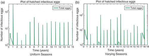
Figure 9. Infected eggs that survive the dry season and hatch at the beginning of the next wet season for the RVF juvenile extension model (9) on a log scale with seasonality. Dry season hatch rate is very low (γ_e=0.005) so that essentially no mosquitoes will hatch during the dry season. Subfigure (a) shows infectious eggs settling to yearly periodic levels, while varying rainfall results in varying numbers of infectious eggs hatching in subfigure (b). Years with large outbreaks result in infectious eggs hatching at significant levels during the wet season as well. (a) Uniform seasons; (b) Varying seasons.

6. Discussion and conclusion

We extended Chitnis et al.’s 9 model to be applicable to RVF by including vertical transmission for Aedes mosquitoes and an asymptomatic class for livestock. The extended model accounts for the population dynamics of both livestock and Aedes mosquitoes and seasonal changes in weather that affects the mosquito population size. Mosquito densities vary greatly over seasons, and the contact rates vary dynamically based upon both the host and mosquito densities 9. We also extended the model to include an aquatic juvenile stage and investigated the sensitivity of our predictions to including this juvenile class. We proved that both models are mathematically and epidemiologically well-posed, analysed the existence and the stability of disease-free equilibrium points, and proved the existence of endemic equilibrium points.

We derived an explicit formula for the basic reproductive number, ₀, and the reactivity index, ₀. We compiled two baseline parameter ranges: one representing a wet season and one representing a dry season or a mitigated wet season. We then used local sensitivity analysis to define the sensitivity indices of ₀ and ₀ and determined which parameters are most important to disease persistence and epidemicity in either the dry or the wet season. We found that including the aquatic stage does not significantly change the qualitative behaviour of the model, or the values of computed indices. However, if more complicated juvenile behaviour such as predation and larval competition were included, the aquatic stage may become more important. We also observed that the relative importance of the parameters in the extended juvenile model was about the same as the original model.

The potential for large outbreaks, or epidemicity, of the system (for RVF parameters) is sensitive to the vector-to-host ratio as well as the mosquito biting rate and the probability of transmission from hosts to vectors. The basic reproductive number, on the other hand, was most sensitive to the mosquito biting rate, the mosquito death rate, and the probability of transmission from vector to host. Neither the basic reproductive number nor the reactivity index were sensitive to vertical transmission in mosquitoes. Adams and Boots 1 also found that the basic reproductive number for their dengue model was not sensitive to vertical transmission in mosquitoes.

The sensitivity analysis suggests that control methods may vary depending on the season and on whether or not the goal is to reduce initial spread and endemicity, or epidemicity (reactivity). We found that ₀ is most sensitive to the mosquito biting rate, the lifetime of a mosquito, and the probability of transmission from vectors to hosts. After these three key parameters, the relative importance of the other model parameters depended upon the choice of wet season or dry season parameters. In the wet season, the next three most important parameters were the probability of transmission from hosts to vectors, the number of bites a host can sustain, and the rate of recovery for infectious hosts. In the dry season, the next most important parameters were the carrying capacities of the mosquitoes and cows, and the probability of transmission from hosts to vectors. These differences can help guide different mitigation strategies in wet and dry seasons.

Controlling the lifespan and biting rate of the mosquitoes will help control both the initial spread of disease and ongoing epidemics. However, if policymakers wish to decrease the probability of a large transient epidemic, reducing the overall numbers of vectors (or the vector-to-host ratio) and the probability of transmission from the host to the vector will be effective. If they wish to reduce the basic reproductive number, it would be better to focus on the probability of transmission from vectors to hosts and on the number of bites a host will sustain.

If the basic reproductive number is less than 1 (as in the dry season case), we showed that the unique disease-free equilibrium is stable. However, the system is still reactive, so transient epidemics are possible even when . If the basic reproductive number is greater than 1 (as in the wet season case), we proved that at least one endemic equilibrium exists. Our numerical simulations suggest that, if introduced to a naive population with wet season parameters, RVF will oscillate between transient large epidemics for several years before settling at a low endemic state. In fact, after the first large epidemic, the number of infected vectors and hosts falls well below 1 for over 2 years due to the large level of herd immunity reached. This indicates that RVF would probably die out after the first big outbreak. In order for RVF to persist between outbreaks, either an infected mosquito or infected host must be introduced to the system at the correct time. It is thought that Aedes mosquito eggs can survive from months to years before hatching at the next flood event. Thus, in regions where there are transient large epidemics, vertical transmission resulting in the hatching of infected mosquitoes could be playing a large role in the inter-epidemic persistence of RVF even if wet season conditions existed year round.

Many RVF epidemics appear to be driven by seasonality. We explored a simple seasonal model to verify that long-term persistence of RVF with marked seasonality requires vertical transmission or introduction from outside the system of an infected host. In fact, if the system is closed, long-term persistence is sensitive to vertical transmission probability, requiring for our scenario a vertical transmission probability of 0.015–0.03 for persistence. These conditions may be relaxed if we expanded the model to include survival of eggs over multiple dry seasons rather than survival over only one dry season. We also considered varying rainfall over wet seasons, which is more realistic for many areas where RVF is endemic or invading. Again, vertical transmission is required for inter-epidemic persistence.

Vertical transmission in mosquitoes is often ignored in models for mosquito-borne pathogens. However, when mosquito populations follow seasonal patterns with large amplitudes, vertical transmission could play a significant role in long-term persistence of a pathogen. These results indicate that further exploration of vertical transmission rates and egg survival from both experimental and modelling perspectives is needed. More in-depth analysis of a seasonal version of the model is also warranted. In the future, we would like to adapt this model to include mitigation strategies and more complex mosquito dynamics, especially as better experimental and field data become available. In conclusion, although vertical transmission does not appear to affect epidemic dynamics significantly, the inter-epidemic persistence of mosquito-borne pathogens can be highly sensitive to vertical transmission rates.

Acknowledgements

This research (C.M. and J.H.) was partially supported by an NIH/NIGMS grant in the Models of Infectious Disease Agent Study (MIDAS) programme, 1U01GM097661-01 and an NSF/MPS/DMS grant DMS-1122666. We thank Kyle S. Hickmann for help with the global sensitivity analysis, and Ling Xue and an anonymous reviewer for valuable comments.

Notes

This paper is based on an invited talk given at the 3rd International Conference on Math Modeling, Analysis, San Antonio, USA, October 2011.

References

- B. Adams, and M. Boots, How important is vertical transmission in mosquitoes for the persistence of dengue? Insights from a mathematical model, Epidemics 2(1) (2010), pp. 1–10 doi: 10.1016/j.epidem.2010.01.001
- S.F. Andriamandimby, A.E. Randrianarivo-Solofoniaina, E.M. Jeanmaire, L. Ravololomanana, L.T. Razafimanantsoa, T. Rakotojoelinandrasana, J. Razainirina, J. Hoffmann, J.P. Ravalohery, J.T. Rafisandratantsoa, P.E. Rollin, and J.M. Reynes, Rift Valley fever during rainy seasons, Madagascar, 2008 and 2009, Emerg. Infect. Dis. 16(6) (2010), pp. 963–970 doi: 10.3201/eid1606.091266
- A. Anyamba, J.P. Chretien, J. Small, C.J. Tucker, P.B. Formenty, J.H. Richardson, S.C. Britch, D.C. Schnabel, R.L. Erickson, and K.J. Linthicum, Prediction of a Rift Valley fever outbreak, Proc. Natl Acad. Sci. 106(3) (2009), pp. 955–959 doi: 10.1073/pnas.0806490106
- L. Arriola, Sensitivity analysis for quantifying uncertainty in mathematical models, Mathematical and Statistical Estimation Approaches in Epidemiology, G. Chowell, J.M. Hyman, L.M.A. Bettencourt, and C. Castillo-Chavez, eds., Springer, New York, 2009, pp. 195–248
- Y. Ba, D. Diallo, C. M.F. Kebe, I. Dia, and M. Diallo, Aspects of bioecology of two Rift Valley fever virus vectors in Senegal (West Africa): Aedes vexans and Culex poicilipes (Diptera: Culicidae), J. Med. Entomol. 42(5) (2005), pp. 739–750 doi: 10.1603/0022-2585(2005)042[0739:AOBOTR]2.0.CO;2
- H.H. Balkhy, and Z.A. Memish, Rift Valley fever: An uninvited zoonosis in the Arabian peninsula, Int. J. Antimicrob. Agents 21(2) (2003), pp. 153–157 doi: 10.1016/S0924-8579(02)00295-9
- B.H. Bird, T.G. Ksiazek, S.T. Nichol, and N.J. MacLachlan, Rift Valley fever virus, J. Am. Vet. Med. Assoc. 234(7) (2009), pp. 883–893 doi: 10.2460/javma.234.7.883
- V. Chevalier, S. Rocque, T. Baldet, L. Vial, and F. Roger, Epidemiological processes involved in the emergence of vector-borne diseases: West Nile fever, Rift Valley fever, Japanese encephalitis and Crimean–Congo haemorrhagic fever, Rev. Sci. Tech. – Office International des Epizooties 23(2) (2004), pp. 535–556
- N. Chitnis, J.M. Cushing, and J.M. Hyman, Bifurcation analysis of a mathematical model for malaria transmission, SIAM J. Appl. Math. 67(1) (2006), pp. 24–45 doi: 10.1137/050638941
- N. Chitnis, J.M. Hyman, and J.M. Cushing, Determining important parameters in the spread of malaria through the sensitivity analysis of a mathematical model, Bull. Math. Biol. 70(5) (2008), pp. 1272–1296 doi: 10.1007/s11538-008-9299-0
- J.M. Cushing, An Introduction to Structured Population Dynamics, CBMS-NSF Regional Conference Series in Applied Mathematics Vol. 71, SIAM, Philadelphia, PA, 1998.
- F.G. Davies, and V. Martin, Recognizing Rift Valley Fever, FAO, Rome, 2003.
- J. M.O. Depinay, C.M. Mbogo, G. Killeen, B. Knols, J. Beier, J. Carlson, J. Dushoff, P. Billingsley, H. Mwambi, J. Githure, A.M. Toure, and F.E. McKenzie, A simulation model of African Anopheles ecology and population dynamics for the analysis of malaria transmission, Malar. J. 3(1) (2004), pp. 29 doi: 10.1186/1475-2875-3-29
- O. Diekmann, J. A.P. Heesterbeek, J. A.J. Metz, On the definition and the computation of the basic reproduction ratio R 0 in models for infectious diseases in heterogeneous populations, J. Math. Biol. 28(4) (1990), pp. 365–382 doi: 10.1007/BF00178324
- C. Favier, K. Chalvet-Monfray, P. Sabatier, R. Lancelot, D. Fontenille, and M.A. Dubois, Rift Valley fever in West Africa: The role of space in endemicity, Trop. Med. Int. Health 11(12) (2006), pp. 1878–1888 doi: 10.1111/j.1365-3156.2006.01746.x
- H.D. Gaff, D.M. Hartley, and N.P. Leahy, An epidemiological model of Rift Valley fever, Electron. J. Differ. Equ. 2007(115) (2007), pp. 1–12
- H. Gaff, C. Burgess, J. Jackson, T. Niu, Y. Papelis, and D. Hartley, Mathematical model to assess the relative effectiveness of Rift Valley fever countermeasures, Int. J. Artif. Life Res. 2(2) (2011), pp. 1–18 doi: 10.4018/jalr.2011040101
- W.A. Geering, F.G. Davies, and V. Martin, Preparation of Rift Valley Fever Contingency Plans, Food & Agriculture Organization of the UN (FAO), Rome, 2002.
- G.H. Gerdes, Rift Valley fever, Rev. Sci. Tech. (International Office of Epizootics) 23(2) (2004), pp. 613–623
- H. Gong, A. DeGaetano, and L.C. Harrington A climate based mosquito population model, Proceedings of the World Congress on Engineering and Computer Science 2007, WCECS 2007, San Francisco, CA, 24–26 October 2007.
- G.R. Hosack, P.A. Rossignol, and P. Van Den Driessche, The control of vector-borne disease epidemics, J. Theor. Biol. 255(1) (2008), pp. 16–25 doi: 10.1016/j.jtbi.2008.07.033
- J.M. Hyman, and J. Li, An intuitive formulation for the reproductive number for the spread of diseases in heterogeneous populations, Math. Biosci. 167(1) (2000), pp. 65–86 doi: 10.1016/S0025-5564(00)00025-0
- P.G. Jupp, A. Kemp, A. Grobbelaar, P. Leman, F.J. Burt, A.M. Alahmed, D. Mujalli, M. Khamees, and R. Swanepoel, The 2000 epidemic of Rift Valley fever in Saudi Arabia: Mosquito vector studies, Med. Vet. Entomol. 16(3) (2002), pp. 245–252 doi: 10.1046/j.1365-2915.2002.00371.x
- T.R. Kasari, D.A. Carr, T.V. Lynn, and J.T. Weaver, Evaluation of pathways for release of Rift Valley fever virus into domestic ruminant livestock, ruminant wildlife, and human populations in the continental United States, J. Am. Vet. Med. Assoc. 232(4) (2008), pp. 514–529 doi: 10.2460/javma.232.4.514
- V. Martin, V. Chevalier, P. Ceccato, A. Anyamba, L. De Simone, J. Lubroth, S. de La Rocque, and J. Domenech, The impact of climate change on the epidemiology and control of Rift Valley fever, Rev. Sci. Tech. – Office International des Epizooties 27 (2008), pp. 413–426
- S.C. Mpeshe, H. Haario, and J.M. Tchuenche, A mathematical model of Rift Valley fever with human host, Acta Biotheor. 59 (2011), 3–4pp. 231–250 doi: 10.1007/s10441-011-9132-2
- R.M. Murithi, P. Munyua, P.M. Ithondeka, J.M. Macharia, A. Hightower, E.T. Luman, R.F. Breiman, and M.K. Njenga, Rift Valley fever in Kenya: History of epizootics and identification of vulnerable districts, Epidemiol. Infect. 139(3) (2011), pp. 372–380 doi: 10.1017/S0950268810001020
- E.J. Muturi, S. Muriu, J. Shililu, J.M. Mwangangi, B.G. Jacob, C. Mbogo, J. Githure, and R.J. Novak, Blood-feeding patterns of Culex quinquefasciatus and other culicines and implications for disease transmission in Mwea rice scheme, Kenya, Parasitol. Res. 102(6) (2008), pp. 1329–1335 doi: 10.1007/s00436-008-0914-7
- P.I. Ndiaye, D.J. Bicout, B. Mondet, and P. Sabatier, Rainfall triggered dynamics of Aedes mosquito aggressiveness, J. Theor. Biol. 243(2) (2006), pp. 222–229 doi: 10.1016/j.jtbi.2006.06.005
- P.I. Ndione, J.P. Besancenot, J.P. Lacaux, and P. Sabatier, Environnement et épidémiologie de la fièvre de la vallée du Rift (FVR) dans le bassin inférieur du fleuve Sénégal, Environnement, Risques & Santé 2(3) (2003), pp. 176–182
- M.G. Neubert, and H. Caswell, Alternatives to resilience for measuring the responses of ecological systems to perturbations, Ecology 78(3) (1997), pp. 653–665 doi: 10.1890/0012-9658(1997)078[0653:ATRFMT]2.0.CO;2
- M. Pépin, M. Bouloy, B.H. Bird, A. Kemp, and J. Paweska, Rift Valley fever virus (Bunyaviridae: Phlebovirus): An update on pathogenesis, molecular epidemiology, vectors, diagnostics and prevention, Vet. Res. 41 (2010), pp. 61 doi: 10.1051/vetres/2010033
- P.H. Rabinowitz, Some global results for nonlinear eigenvalue problems, J. Funct. Anal. 7 (1971), pp. 487–513 doi: 10.1016/0022-1236(71)90030-9
- W.S. Romoser, M.N. Oviedo, K. Lerdthusnee, L.A. Patrican, M.J. Turell, D.J. Dohm, K.J. Linthicum, and C.L. Bailey, Rift Valley fever virus-infected mosquito ova and associated pathology: Possible implications for endemic maintenance, Res. Rep. Trop. Med. 2 (2011), pp. 121–127 doi: 10.2147/RRTM.S13947
- P.A. Rossignol, J.M. Ribeiro, M. Jungery, M.J. Turell, A. Spielman, and C.L. Bailey, Enhanced mosquito blood-finding success on parasitemic hosts: Evidence for vector-parasite mutualism, Proc. Natl Acad. Sci. USA 82(22) (1985), pp. 7725–7727 doi: 10.1073/pnas.82.22.7725
- J. Shaman, and J.F. Day, Reproductive phase locking of mosquito populations in response to rainfall frequency, PloS One 2(3) (2007), pp. e331 doi: 10.1371/journal.pone.0000331
- M.J. Turell, C.A. Rossi, and C.L. Bailey, Effect of extrinsic incubation temperature on the ability of Aedes taeniorhynchus and Culex pipiens to transmit Rift Valley fever virus, Am. J. Trop. Med. Hyg. 34(6) (1985), pp. 1211–1218
- M.J. Turell, S.M. Presley, A.M. Gad, S.E. Cope, D.J. Dohm, J.C. Morrill, and R.R. Arthur, Vector competence of Egyptian mosquitoes for Rift Valley fever virus, Am. J. Trop. Med. Hyg. 54(2) (1996), pp. 136–139
- M.J. Turell, K.J. Linthicum, L.A. Patrican, F.G. Davies, A. Kairo, and C.L. Bailey, Vector competence of selected African mosquito (diptera: Culicidae) species for Rift Valley fever virus, J. Med. Entomol. 45(1) (2008), pp. 102–108 doi: 10.1603/0022-2585(2008)45[102:VCOSAM]2.0.CO;2
- P. Van den Driessche, and J. Watmough, Reproduction numbers and sub-threshold endemic equilibria for compartmental models of disease transmission, Math. Biosci. 180(1) (2002), pp. 29–48 doi: 10.1016/S0025-5564(02)00108-6
- C. Vignolles, J.P. Lacaux, Y.M. Tourre, G. Bigeard, J.A. Ndione, and M. Lafaye, Rift Valley fever in a zone potentially occupied by Aedes vexans in Senegal: Dynamics and risk mapping, Geospatial Health 3(2) (2009), pp. 211–220
- L. Xue, H.M. Scott, L.W. Cohnstaedt, and C. Scoglio, A network-based meta-population approach to model Rift Valley fever epidemics, J. Theor. Biol. 306 (2012), pp. 129–144 doi: 10.1016/j.jtbi.2012.04.029