A deterministic model for influenza infection with multiple strains and antigenic drift

Abstract

We describe a multiple strain Susceptible Infected Recovered deterministic model for the spread of an influenza subtype within a population. The model incorporates appearance of new strains due to antigenic drift, and partial immunity to reinfection with related circulating strains. It also includes optional seasonal forcing of the transmission rate of the virus, which allows for comparison between temperate zones and the tropics. Our model is capable of reproducing observed qualitative patterns such as the overall annual outbreaks in the temperate region, a reduced magnitude and an increased frequency of outbreaks in the tropics, and the herald wave phenomenon. Our approach to modelling antigenic drift is novel and further modifications of this model may help improve the understanding of complex influenza dynamics.

Keywords:

• influenza
• antigenic drift
• cross-immunity
• multiple strains
• seasonality

AMS Subject Classification:

• 92D30
• 92D15

1. Introduction

Influenza presents a significant morbidity and mortality burden in the world; a typical seasonal influenza epidemic kills up to 49,000 people per year [5] in the USA, and from a quarter to half a million worldwide [27]. One of the key aspects of the influenza virus is its ability to reinfect hosts. Influenza is an RNA virus and lacks a proofreading mechanism for its polymerase. As a consequence, it is prone to mistakes every time a copy of its genome is made. Since these mutations usually do not change how the virus is identified by the immune system, an infection with one influenza strain generally confers lasting immunity to an identical strain. However, if the virus has undergone sufficient significant changes in its surface proteins, then reinfection with influenza is possible. This process is termed antigenic drift. One of the main findings on this topic is that the immunity conferred after infection wanes with decreasing relatedness between the immunizing and challenging strains [7]. Thus, once a few years have passed since the previous infection with a specific subtype of influenza, a human host may become almost completely susceptible to the currently circulating grand-daughter strain [7].

The main challenge in influenza control is an early prediction of the strain that will be the dominant circulating one each season. This is needed so that a matching vaccine can be mass produced on time. ‘Herald’ waves of influenza (strains which begin to dominate very late in a previous season) have been successfully used many times in the past to develop the following year's vaccines [10,19]. A model of influenza dynamics that can provide useful information about the persistence of strains from season to season would be helpful to improve the success rates of vaccines. Such a model would ideally take into account several key biological features including the drift process (via the emergence of new strains), the co-circulation of related strains, and pre-existing immunity in the population. The current model is an initial step towards a more general model.

Influenza has been widely studied and characterized for temperate regions. The occurrence shows significant seasonal variations with marked peaks in the winter season each year [26]. In contrast, influenza seasonality is less defined in the tropics, where a viral strain may persist in the population throughout the entire year at a constant intermediate level, with some peaks varying from country to country [1,22,25], and no distinct annual patterns [1,15,21]. We applied our model to both regions and obtained similar results.

An excellent overview of early modelling work involving the dynamics of influenza drift can be found in Andreasen [2]. The models of Andreasen [2], Boni et al. [4], and Ferguson et al. [8] incorporate seasonality in the modelling of influenza. The former two models are deterministic and only consider one strain per season. Immunity to the next strain is set up based on the past epidemic dynamics. In this sense, these models are most suitable for temperate regions that have a fixed annual cycle of influenza seasons. The model in Ferguson [8] incorporates seasonality via harmonic forcing of the transmission rate and it thus more suitable to be applied to any region, including tropics. However, the model is computationally intensive, and thus may not be suitable for routine modelling in large populations.

Work by Gog and colleagues has focused on multiple strains during one epidemic (see, for example, [13], which also includes a recent review of multi-strain models). In this paper we take a different approach than that of Gog, and model the dynamics over several seasons, with simpler assumptions on the transmission rates.

Earlier work by Gog and Grenfell [11] or Lin and Andreasen [16] establish a one-dimensional space (discrete and continuous, respectively) where the strains of influenza might mutate. In this work we take a different approach and consider only distances between strains and relationships between mother and daughter strains, but we do not associate them with a one-dimensional space.

We describe a deterministic susceptible infected recovered type model for the spread of seasonal influenza. The model incorporates the appearance of new strains and partial immunity due to prior infections with related strains. Because seasonality is important to consider in temperate regions, our model includes optional seasonal forcing of the transmission rate.

The main results of this study show that our model is capable of successfully capturing several key features in influenza data, including: (1) the reduced annual attack rate and more frequent epidemic peaks in the tropics compared with temperate regions [1,15,21], (2) the overall observed attack rate, and (3) the annual peaks in genetic diversity during winter in temperate regions that are interspersed by bottlenecks in diversity during summer months [20]. The model also successfully reproduces the herald wave phenomenon of strain persistence from one influenza season to the next in temperate regions.

2. Model

The model described here focuses on a certain subtype of influenza of type A (e.g. influenza A(H1N1), A(H3N2)) or influenza of type B. The main reason for this consideration is that we intend to study the dynamics of the drift process of influenza. The infection process is described by a susceptible infected recovered model, in which individuals are divided into classes according to the history of infections by strains that had previously circulated or are currently circulating. The infection rate for individuals in each of the classes may change depending on how closely related the strains are in an antigenic map.

We assume that when there are enough individuals infected with a certain strain, a new mutation closely related to that circulating strain will appear, at which time the model will be updated to incorporate the new strain.

2.1. Notation for the epidemiological classes

Consider the case when n strains are currently co-circulating in a population. We divide the population into epidemiological classes according to the infection history of individuals. Let v=(v₁, v₂, …, v_n) be a vector which keeps track of the infection history of an individual. The components of v are either one or zero; with v_i=1 and v_i=0 representing whether or not the individual has already been infected by the virus strain i, respectively. A vector of this type will be referred to as a history vector. Note that the total number of possible history vectors is 2ⁿ. We will use R_v to denote the recovered class with history v. Note that R0=R_{(0, …, 0)} represents the completely susceptible class. To avoid any confusion between R0 and the usual notation for the basic reproduction ratio, we will use S to replace R_{(0, …, 0)} in the model description.

For the infected classes, we need to keep track of the information on both the strain of current infection and the infection history. Let denote the infected class which includes all individuals who are currently infected with strain i and have the history v. For example, if n=3, an individual in is currently infected with strain 1 and was previously infected with strain 3 but not strain 2. Note that if an individual is infected with strain i it necessarily has a one on position i of its history vector, thus, for example is not a possible class. So, in the case of n strains, there are n2ⁿ⁻¹ infected classes.

2.2. Transitions between classes

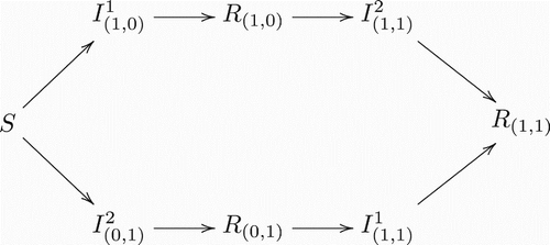
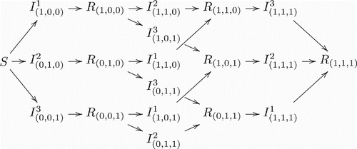
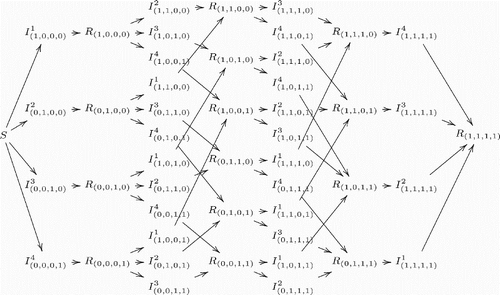
Figures 1–4 illustrate the model structure by exhibiting different scenarios for different numbers of co-circulating strains in a population. It is clear that the complexity of model structure increases significantly when the number of co-circulating strains increases. However, the basic patterns are straightforward and the rules remain the same for arbitrary numbers of co-circulating strains. An individual in (who is currently infected with strain i and has history v) recovers and enters in the recovered class R_v with the same history v. On the other hand, new infections entering in the class have to come from the recovered class R_v′, where v′ denotes the history vector that is the same as v except that v_i=0. Here, it is assumed that individuals who recover from an infection by strain i will have permanent immunity against the same strain.

Figure 1. Transitions between classes when there is only one strain present. Notice this is a regular Susceptible-Infected-Recovered model.

Figure 2. Transitions between classes with two co-circulating strains.

Figure 3. Transitions between classes with three co-circulating strains.

Figure 4. Transitions between classes with four co-circulating strains.

Vital dynamics are also considered in our model. For simplicity, we assume a constant total population size. We denote by μ the natural death rate (equal to the birth rate) for all epidemiological classes in the model.

2.3. Time-dependent rate of disease transmission

Although the reason for seasonal variations in influenza in the temperate regions is not well understood, one of the major driving forces appears to be the time-dependent transmission rate of the disease [17]. In our model, the transmission rate is assumed to be a time-dependent periodic function defined by where βˆ_i is a constant background transmission rate of strain i, which also represents the constant transmission rate in the absence of seasonality (i.e. ϵ=0). If t=0 corresponds to January 1st of a calendar year, then the β(t) function with ϵ>0 corresponds to the northern hemisphere, implying that the transmission rate is higher in the winter, on dates that are close to January 1st. On the other hand, if ϵ<0, then the transmission will be biggest on dates close to the middle of the year, which corresponds to the winter on the southern hemisphere. The case of ϵ=0, or a value close to 0, corresponds to a model for the tropics.

This function should be understood as an approximation of what happens in reality. If more data on other factors that influence seasonality are known, the function could be made to depend on these parameters. There must be some seasonality linked to tropical regions as well, probably linked to rainy seasons, and more factors that influence the seasonality in temperate regions [17]; but for simplicity we will assume that seasonality is small enough in the tropics and that the function looks like the one in Equation (1).

2.4. Cross-immunity

For an individual in the class R_v with v_i=0 (i.e. the individual has not been previously infected by this strain), the cross-immunity against a strain i will depend on the individual's history. We define the distance between strain i and the history vector v by considering the antigenic distance between strains i and j for all j with v_j=1.

Various definitions have been used previously to define the distance between two strains (see [8,14]). We point out that we do not intend to consider the genetic distance between the strains, but rather the antigenic distance (for a very good distinction between both concepts for the particular case of influenza, see Smith, et al. [23]). We follow here the approach of Ferguson, et al. [8] by considering that if strain i originates by a mutation of strain j, then these two strains will have a small distance between them. And the less ‘related’ the strains are, the farther their distance is.

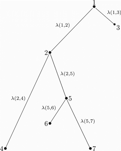
Suppose that it is possible to measure the antigenic distance between a strain and its progenitor (more on this subject will be discussed in Section 2.6). The distance between strains i and j will then be associated with the closest path joining these two strains in the phylogenetic tree of the subtype of influenza. We can identify the first strain that is a common ancestor of both i and j, then add up all the distances from i to this common ancestor and from j to this common ancestor. The sum of these distances can be used to define the distance between strains i and j, which we denote by λ(i, j). We define λ(i, i)=0.

The definition of this distance can be better explained by using the example illustrated in Figure 5, which shows a hypothetical phylogenetic tree for seven strains of influenza. In this figure, strains 2 and 3 mutated from a common progenitor, strain 1. Strain 2 generated strains 4 and 5, and strain 5 later generated strains 6 and 7. To calculate the distance between strains 4 and 6, we notice that the first common ancestor of both 4 and 6 is strain 2. The distance then is λ(4, 6)=λ(2, 4)+λ(2, 5)+λ(5, 6).

Figure 5. Hypothetical phylogenetic tree of seven influenza strains.

These distances will then be used to define cross-immunity as follows. The effect of cross-immunity is reflected by a reduction in the transmission rates. Following the approach of Boni et al. [4], we define the cross-immunity to be a decaying function, e^{−λ(i, j)}, of the distance λ(i, j). For an individual who had previously been infected with strain j, the infectivity by strain i is reduced by a factor defined by so that the transmission rate is 0 in the case of total immunity and it is β_i(t) in the case of complete susceptibility.

To define the level of protection that a given class v has against strain i, we use the best protection in the history of previous infections of that class, that is, where H(v) is the set of all strains that individuals with history v had previously been infected with, i.e.

Then, the transmission rate by strain i for individuals in the Rv class will be reduced to ρ vⁱ β_i(t).

2.5. Model equations with n co-circulating strains

Using the notations defined in previous sections, our system of differential equations for the case of n strains reads for v≠0; where, ‘x˙’ denotes dx/dt and N is the total population: which remains constant for all time t, since N˙=0.

Since there are 2ⁿ recovered classes (including S) and 2ⁿ⁻¹n infected classes, the total number of equations in this system is 2ⁿ⁻¹(n+2) for n circulating strains.

2.6. Addition of a new strain in system (5)

A unique feature of our modelling approach is to allow the addition of new strains generated from mutations. Our idea is based on the fact that for a given strain i, the probability that a new strain develops in an infected individual is relatively similar for each infected individual. So at a given moment of time, the probability of having a mutation of a new strain just depends on the cumulative number of infected individuals.

We assume that when a new strain j is mutated from strain i, a new set of equations associated with strain j will be added, and System (5) will be updated accordingly. The number of individuals in the class will not be reduced because of the introduction of an individual with the new strain j.

The second assumption is about the criterion on the timing for the introduction of a new strain. Based on the understanding that the likelihood of a significant mutation responsible for creating a new strain can be thought to be an independent process for each infection, it is reasonable to assume that the mean time for a new strain to appear depends mainly on the cumulative number of infections of a previously created strain i. This threshold number, which we denote by , will be used to determine the time for a new strain to appear. Specifically, let denote the number of new infections of strain i between the time a and the time b, then Let t₁>0 denote the time at which the last daughter strain of strain i was generated (or the time at which the strain i was generated if it still does not have a daughter strain). Then a new strain will be created at time t₂ if ; that is, This will increase the number of strains to n+1.

We point out that although the threshold condition for strain creation given by Equation (7) is defined in a deterministic way, it can be easily modified by considering the condition to be stochastic.

For the added (n+1) strain, which was mutated from the mother strain i, we need to define the distance between these two strains λ(i, n+1). In our case, we set this distance to be a fixed constant λ, i.e. λ(i, n+1)=λ, but other stochastic functions could also be used. The (n+1) strain will add one more node to the phylogenetic tree, and we need to calculate the distances between the nodes again. Notice that changes in the distances occur only in those values of λ(j, k) with either j=n+1 or k=n+1. Since λ(j, k)=λ(k, j), we only need to calculate the new values of λ(j, n+1) for all j≠i. We have Using Equation (8) we can update the cross-immunity defined in Equation (3) for all j≤n+1 and all history vectors v of dimension n+1.

We also need to determine the other parameter values for the new strain, the transmission coefficient β_n+1 and the recovery rate γ_n+1. In the case of a deterministic model, one simple way is to define Note that under this definition, if we start with a single strain with values β and γ, then these values will remain the same for all new strains. If stochastic influences are to be considered in the model, β_n+1 and γ_n+1 can be random, e.g. drawn from normal distributions with means β_i and γ_i, respectively.

2.7. Update of equations in the (n+1)-strains system

Once the model parameters have been updated as described in the previous sections, the equations for the new (n+1)-strains system will have the same form as those in System (5), except that the history vectors are now of dimension n+1. The total number of equations will increase from 2ⁿ⁻¹(n+2) to 2ⁿ(n+3).

The initial conditions also need to be updated for t≥t₂, where t₂ is the time at which the new strain was created (see Equation (7)). Let z denote the history vector of dimension n for which (z, 1) corresponds to the individual who is the first person carrying the new strain. A deterministic approach for defining z is to choose the history vector for which the value is the largest. In a stochastic setting, we could just sample a distribution with the probability mass function . Using these notations, the new initial conditions can be described as

The new equations for the (n+1)-strain system will be used for t>t₂ until the (n+2) strain appears at some time t>t₂, at which time the system of (n+1)-strains will be extended to a new system of (n+2)-strains following the same rules described above.

3. Model simulations and results

Because of the need to track the history of co-circulating strains in the population, the model will have a large number of equations. This fact and a time-dependent transmission rate make analytic studies of the model very difficult. Thus, the results presented here are based mainly on numerical simulations. Detailed descriptions of the methods used in the simulations and the main results are provided below.

3.1. Initialization of parameters

For the initialization of model parameters, we simulate influenza transmission over many years in a population of ten million individuals in both the tropics (ϵ=0 in Equation (1)) and northern temperate regions (positive values of ϵ). We start the simulation at time t=0 with only one strain and a small number of infected individuals. The seasonal forcing of influenza is currently unknown and has not been extensively studied. However, a few data and modelling studies indicate that values of 0.20–0.35 for ϵ appear to be reasonable estimates [8,24]. Here, we assume values of ϵ to vary between 0 and 0.20 and try to get an insight into the transition from a tropical region to a temperate one.

The basic reproduction ratio of influenza has been measured in temperate climates to be between 1.1 and 1.7, with an average around 1.4 [3,9]. We assume that these estimates occur in the winter when the transmission rate is maximal. We thus estimate the baseline transmission rate in Equation (1) to be , where γ is the recovery rate with 1/γ=3 (i.e. the infectious period is three days) [6].

The parameters for the threshold value defined in Equation (7) and the antigenic distance λ are calibrated based on the following considerations. We select the parameter values for which sustained dynamic resonance is achieved in all populations, without an unnaturally high annual attack rate or an over-abundance of co-circulating strains (which we found to be associated with a high attack rate). We take the unnaturally high attack rate to be 50% for the temperate regions, given that the maximal observed clinical attack rate is estimated to be 25% [18], but up to 60% of such infections are asymptomatic [12]. We find that for between 25% and 38% of the population, and λ between 1.5 and 1.8, the simulations yield sustained resonance in both the tropics and temperate regions.

3.2. Results

Here, we present a set of simulations from our model that are capable of capturing the observed patterns of influenza prevalence in the two regions, tropical and temperate. The parameter values used in the simulations are identical for all the regions except for the transmission rates, for which a constant (or close to constant) rate is used for the tropic region while a periodic function is chosen for the different temperate regions. Most of the parameter values are chosen based on the discussion in Section 3.1. The simulations are for a period of 25 years.

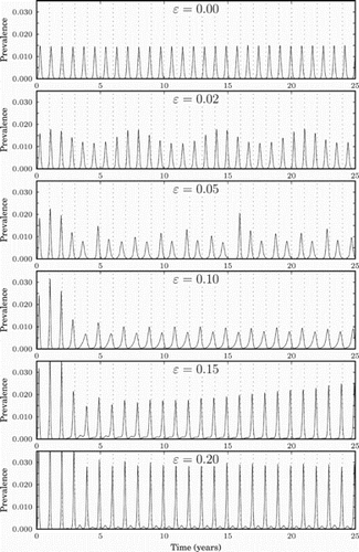
To demonstrate the difference in influenza prevalence curves between tropical and temperate regions, we illustrate in Figure 6 the simulation results for various values of ϵ. Zero or smaller values of ϵ represent the tropical region, whereas larger values represent temperate regions. The figure shows that the size of the epidemic peaks in the tropics is lower than in the temperate region, and that they occur more frequently than annually, matching the pattern that is seen in data (lower peaks more frequently [1,15,21]). The figure also presents diversity bottlenecks each summer, a pattern that is observed in data [20]. The parameter values used are: γ=days⁻¹, (that is 27% of the total population) and λ=1.5.

Figure 6. Prevalence (measured in percentage of the population infected per day) for different values of non-negative ϵ, i.e. for the tropics and the northern hemisphere. The dashed vertical lines represent the middle of the winter of each year.

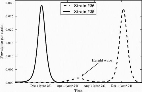
The herald wave phenomenon observed in data is reproduced in our model when applied to a temperate region (e.g. for the value of ϵ=0.20), with the strain that dominates each season appearing late in the previous season (Figure 7). The overall average annual attack rate in the temperate region with this set of parameters was around 45%, leading to an estimated clinical attack rate of around 18% [12].

Figure 7. The herald wave phenomenon. A summer wave of a new strain predicts the strain that will dominate over the following winter. The value of seasonal forcing used is ϵ=0.20. Prevalence for each strain is measured in percentage of the population infected per day.

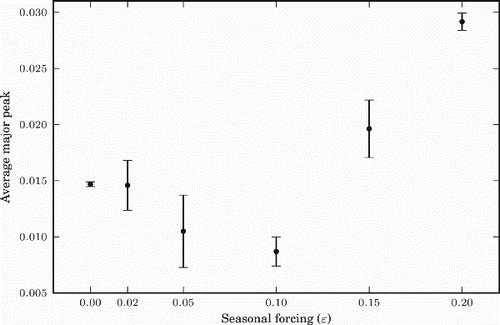
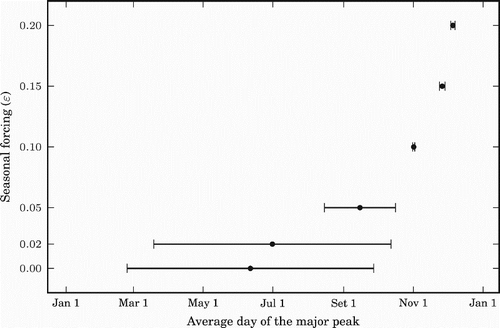
To examine how the seasonal forcing (ϵ) may affect the size of annual major peak of influenza prevalence and the timing of the peak, we plotted in Figures 8 and 9, for different values of ϵ, the average peak and average date of the peaks, respectively, over a period of 20 years (starting four and half years after the initialization of the model). The standard deviation is also indicated for each fixed ϵ value. In these figures, the case of ϵ=0 (or smaller ϵ values) corresponds to the tropics and the cases of larger positive ϵ correspond to the northern hemisphere. Figure 8 shows that the size of the major peak decreases first with ϵ and increases for larger ϵ. Figure 9 shows that as ϵ gets larger, the timing of the major peak per year shows less difference, naturally in the middle of the winter where the seasonal forcing is biggest. Due to the symmetric property of the model, the same results are true, mutatis mutandis, for the southern hemisphere (negative values of ϵ). These results agree with the data presented in Alonso et al. [1], if we associate ϵ with latitude.

Figure 8. Average size and standard deviation of the major annual peak for different non-negative values of ϵ, i.e. for the tropics and the northern hemisphere.

Figure 9. Average day and standard deviation of the major annual peak for different non-negative values of ϵ, i.e. for the tropics and the northern hemisphere.

4. Discussion

In this paper, we introduced a novel deterministic susceptible, infected, recovered model that mimics the antigenic drift process for influenza. We provide a detailed explanation with a simple notation for a generic model with n strains and a novel way to include the appearance of new strains due to virus mutation, which can be used to model antigenic drift. We illustrated that, with suitable parameter values, the same model is capable of capturing the observed influenza patterns in both temperate and tropical regions.

Our simulation results suggest that the seasonal variation might be responsible for observed patterns in influenza including: (i) higher frequency of disease recurrence in tropical regions than in the temperate regions (annual); (ii) reduced magnitude of disease outbreaks in tropical regions than in temperate regions [1,15,21]; and (iii) annual peaks during winter in temperate regions that are interspersed by bottlenecks of emerging strains during summer months [20]. Since our model does not take into account other very important factors that can influence seasonality as discussed in Section 2.3, it cannot predict what would happen in a particular region. Nevertheless, it can serve as a scheme for such a model, if a better function β(t), that includes those factors, is used.

We remark that we used the same values for the transmission rate for all strains in our simulations, therefore the significant differences in disease outbreaks from season to season are not associated with how infectious the strains are, but with what types of strains the population had encounter before and how close related they are with the one that is currently circulating.

The model is also capable of generating a type of herald wave phenomenon of strain persistence from one influenza season to the next in temperate regions [10,19]. The herald wave phenomenon plays an important role in determining possible strains for the production of vaccine for the following season. Our model is based in only one subtype of influenza. Since the vaccine for influenza generally includes one strain for two subtypes of influenza A and one strain for influenza B, it would be interesting to modify our model to include vaccination and several subtypes; in order to test what could happen if one strain that will circulate is left out of the vaccine.

It has been hypothesized that tropical populations form a source of influenza strains that seed influenza epidemics in temperate regions each season [20]. It would thus be interesting to extend our model to include interactions between tropical and temperate populations to answer questions such as (1) which strains tend to dominate a season in temperate regions? (2) what are the herald wave strains from previous seasons in the same region? and (3) are there possible imported strains from tropical regions?

There are many interesting questions to be explored, and the framework of this model enhances the possibilities for a better understanding of the many complexities of influenza dynamics.

Acknowledgements

We thank the reviewers for helpful comments. The initial idea for this work started during a summer program of the Mathematical and Theoretical Biology Institute (MTBI); we thank all institutions and persons that make MTBI possible. We also thank Carlos Castillo-Chavez for continued discussions and helpful suggestions. This work is partially supported by the NSF grant DMS-1022758.

References

- W. Alonso, C. Viboud, L. Simonsen, E. Hirano, L. Daufenbach, and M. Miller, Seasonality of influenza in Brazil: A traveling wave from the Amazon to the subtropics, Amer. J. Epidemiol. 165 (2007), pp. 1434–1442 doi: 10.1093/aje/kwm012
- V. Andreasen, Dynamics of annual influenza A epidemics with immuno-selection, J. Math. Biol. 46 (2003), pp. 504–536 doi: 10.1007/s00285-002-0186-2
- E. Bonabeau, L. Toubiana, and A. Flahault, The geographical spread of influenza, Proc. Roy. Soc. London Ser. B: Biol. Sci. 265 (1998), pp. 2421–2425 doi: 10.1098/rspb.1998.0593
- M. Boni, J. Gog, V. Andreasen, and F. Christiansen, Influenza drift and epidemic size: The race between generating and escaping immunity, Theoret. Popul. Biol. 65 (2004), pp. 179–191 doi: 10.1016/j.tpb.2003.10.002
- Centers for Disease Control and Prevention, Key facts about seasonal flu vaccine (2012). Available at http://www.cdc.gov/flu/protect/keyfacts.htm.
- V. Colizza, A. Barrat, M. Barthelemy, A. Valleron, and A. Vespignani, Modeling the worldwide spread of pandemic influenza: Baseline case and containment interventions, PLoS Med. 4 (2007), pp. e13 doi: 10.1371/journal.pmed.0040013
- R. Couch, and J. Kasel, Immunity to influenza in man, Ann. Rev. Microbiol. 37 (1983), pp. 529–549 doi: 10.1146/annurev.mi.37.100183.002525
- N. Ferguson, A. Galvani, and R. Bush, Ecological and immunological determinants of influenza evolution, Nature 422 (2003), pp. 428–433 doi: 10.1038/nature01509
- A. Flahault, S. Letrait, P. Blin, S. Hazout, J. Menares, and A. Valleron, Modelling the 1985 influenza epidemic in France, Statist. Med. 7 (1988), pp. 1147–1155 doi: 10.1002/sim.4780071107
- W. Glezen, R. Couch, and H. Six, The influenza herald wave, Amer. J. Epidemiol. 116 (1982), pp. 589–598
- J. R. Gog and B.T. Grenfell, Dynamics and selection of many-strain pathogens, Proc. Nat. Acad. Sci. 99 (2002), pp. 17209–17214 doi: 10.1073/pnas.252512799
- J. King Jr, C. Haugh, W. Dupont, J. Thompson, P. Wright, and K. Edwards, Laboratory and epidemiologic assessment of a recent influenza B outbreak, J. Med. Virol. 25 (1988), pp. 361–368 doi: 10.1002/jmv.1890250313
- A. Kucharski and J.R. Gog, Influenza emergence in the face of evolutionary constraints, Proc. Roy. Soc. B: Biol. Sci. 279 (2012), pp. 645–652 doi: 10.1098/rspb.2011.1168
- A. Lapedes, and R. Farber, The geometry of shape space: Application to influenza, J. Theoret. Biol. 212 (2001), pp. 57–69 doi: 10.1006/jtbi.2001.2347
- V. Lee, J. Yap, J. Ong, K. Chan, R. Lin, S. Chan, K. Goh, Y. Leo, I. Mark, and C. Chen, Influenza excess mortality from 1950–2000 in tropical Singapore, PLoS One 4 (2009), pp. e8096 doi: 10.1371/journal.pone.0008096
- J. Lin, V. Andreasen, R. Casagrandi, and S.A. Levin, Traveling waves in a model of influenza a drift, J. Theoret. Biol. 222 (2003), pp. 437–445 doi: 10.1016/S0022-5193(03)00056-0
- M. Lipsitch, and C. Viboud, Influenza seasonality: Lifting the fog, Proc. Nat. Acad. Sci. USA 106 (2009), pp. 3645–3646 doi: 10.1073/pnas.0900933106
- N. Molinari, I. Ortega-Sanchez, M. Messonnier, W. Thompson, P. Wortley, E. Weintraub, and C. Bridges, The annual impact of seasonal influenza in the US: Measuring disease burden and costs, Vaccine 25 (2007), pp. 5086–5096 doi: 10.1016/j.vaccine.2007.03.046
- S. Nakajima, F. Nishikawa, K. Nakamura, and K. Nakajima, Comparison of the HA genes of type B influenza viruses in herald waves and later epidemic seasons, Epidemiol. Infect. 109 (1992), pp. 559–568 doi: 10.1017/S0950268800050548
- A. Rambaut, O. Pybus, M. Nelson, C. Viboud, J. Taubenberger, and E. Holmes, The genomic and epidemiological dynamics of human influenza A virus, Nature 453 (2008), pp. 615–619 doi: 10.1038/nature06945
- C. A. Russell, T.C. Jones, I.G. Barr, N.J. Cox, R.J. Garten, V. Gregory, I.D. Gust, A.W. Hampson, A.J. Hay, A.C. Hurt, J.C. de Jong, A. Kelso, A.I. Klimov, T. Kageyama, N. Komadina, A.S. Lapedes, Y.P. Lin, A. Mosterin, M. Obuchi, T. Odagiri, A.D.M.E. Osterhaus, G.F. Rimmelzwaan, M.W. Shaw, E. Skepner, K. Stohr, M. Tashiro, R.A.M. Fouchier, and D.J. Smith, The global circulation of seasonal influenza A (H3N2) viruses, Science 320 (2008), pp. 340–346 doi: 10.1126/science.1154137
- J. Simmerman, P. Thawatsupha, D. Kingnate, K. Fukuda, A. Chaising, and S. Dowell, Influenza in Thailand: A case study for middle income countries, Vaccine 23 (2004), pp. 182–187 doi: 10.1016/j.vaccine.2004.05.025
- D. Smith, A. Lapedes, J. Jongde, T. Bestebroer, G. Rimmelzwaan, A. Osterhaus, and R. Fouchier, Mapping the antigenic and genetic evolution of influenza virus, Science 305 (2004), pp. 371–376 doi: 10.1126/science.1097211
- S. Towers, and Z. Feng, Pandemic H1N1 influenza: Predicting the course of a pandemic and assessing the efficacy of the planned vaccination programme in the United States, Eurosurveillance 14 (2009), pp. pii=19358
- C. Viboud, W. Alonso, and L. Simonsen, Influenza in tropical regions, PLoS Med. 3 (2006), pp. e89 doi: 10.1371/journal.pmed.0030089
- C. Viboud, O. Bjornstad, D. Smith, L. Simonsen, M. Miller, and B. Grenfell, Synchrony, waves, and spatial hierarchies in the spread of influenza, Science 312 (2006), pp. 447–451 doi: 10.1126/science.1125237
- WHO, Fact sheet Number 211 (2009), Influenza. Available at http://www.who.int/mediacentre/factsheets/fs211/