Hierarchical competition models with Allee effects

Abstract

We consider a two-species hierarchical competition model with a strong Allee effect. The Allee effect is assumed to be caused by predator saturation. Moreover, we assume that there is a ‘silverback’ species x that gets first choice of the resources and where growth is limited by its own intraspecific competition, while the second ‘inferior’ species y gets whatever is left. Both species x and y are assumed to have the property of strong Allee effect. In this paper we determine the impact of the presence of the Allee effect on the global dynamics of both species.

Keywords:

• extinction region
• Allee effect
• hierarchical
• persistence (coexistence) region
• exclusion region
• stability

2010 AMS Subject Classifications::

• 39A11
• 92D25

1. Introduction

Hierarchical models have been investigated by many authors. Competition hierarchical models were studied by Best and Castillo-Chavez [4], Henson and Cushing [13], and Kinzig et al. [15]. Kinzig et al. [15], Blayneh [5] and Cushing [8,9] investigated hierarchical size-structured population models. In such models, it is assumed that one of the species is a ‘silverback’ species that gets first choice of the resources and whose growth is limited only by its own intraspecific competition, while the second ‘inferior’ species gets whatever resources are left. The above-mentioned studies assume that there is a negative correlation between population density (size) and its per capita growth rate, that is, populations do not possess the Allee effect.

In this paper we assume that both species display the Allee effect. Allee [1] characterized the Allee effect as a phenomenon in ecology where there is a positive correlation between population density (size) and its per capita growth rate. A population would have a strong Allee effect if its positive density dependence is stronger than its negative density dependence. Hence for single-species models, a strong Allee effect is characterized by the presence of a threshold size (density) called the threshold Allee point and sometimes denoted by A, below which, the population would go extinct [2,7,10,12,17,20,22,24]. A more precise definition of the strong Allee effect was given in [18]: indeed, let x_t be the population or density at time period or generation t. Let the fitness φ of species x be defined as the ‘per capita’ growth rate of the population as $\phi (x_t)=x_{t+1}/x_t$, where φ∈C¹, so that the dynamics of the population is given by the difference equation

$x_{t+1}=f(x_t)=x_t\cdot \phi (x_t)\text{with }f(x)=x\cdot \phi (x).$

Then a single-species whose population dynamics is given as in model (1) is said to display the strong Allee effect if the following conditions hold true:

• (i) φ′(x)>0 for $x\in (0,ϵ)$ for some ε>0.

• (ii) φ(0)<1.

• (iii) There exists a unique K>0 such that φ(K)=1 and φ′(K)<0.

Note that from the above conditions, there exists a fixed point A such that $\phi (A)=1,0<A<K,$ and A is unstable. (See Figure 2 and for comparison, we include Figure 1 for the non-Allee effect case.)

Figure 1. A single-species model with no Allee effect. (a) We plot x_t+1=f(x_t). There are two fixed points: $x_1^{\ast }=0$ and $x_2^{\ast }=K$ (the carrying capacity) and (b) we plot the ‘overall’ fitness function x_t+1/x_t versus x_t. Notice that when x_t=K, the fitness function is equal to 1. Moreover, x_t+1/x_t>1.

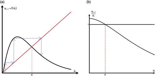
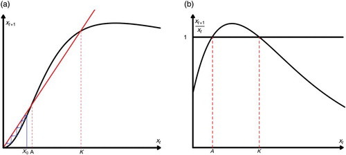
Figure 2. A single-species model with Allee effect. (a) We plot x_t+1=f(x_t). We have two possible fixed points: A (threshold Allee point) and K (carrying capacity). If the population falls below the value of A, it will go extinct and (b) we plot the ‘overall’ fitness function x_t+1/x_t. Notice that x_t+1/x_t|_x=0=1 which is the hallmark of the strong Allee effect.

Allee effects in two-species models were studied in [8,14,18,19]. Strong Allee effect in multi-species models is characterized by the presence of an extinction region where both species would go to extinction if their densities (sizes) fall into that region [18,19]. For instance, a planar competition model is said to display the strong Allee effect property if its phase space exhibits an extinction region and a non-extinction region separated by an Allee threshold curve (a manifold of dimension n−1 where n is the dimension of the phase space).

In this paper we will study two-species hierarchical competition models with the Allee effects. As far as we know this is the first study of these types of models. Our aim is to determine the global dynamics of these systems. In particular, we will determine the regions of extinction, exclusion, and coexistence of both species. We will show that there are five different scenarios: no interior fixed points with unbounded extinction region, one interior fixed point with a semistable centre manifold, two interior fixed points, one is a repeller and the other is a saddle, three interior fixed points, a repeller, a saddle and a third with a stable centre manifold, and four interior fixed points, a repeller, a saddle, a saddle and an attractor. Moreover, persistence of both species occurs only if there are three or four interior fixed points.

2. The single-species model

Let us consider the following single-species Ricker [21] model with the strong Allee effect:

$x_{t+1}=x_t{\mathrm{e}}^{r-x_t-m/(1+s{x}_t)}$

which can be written as

$x_{t+1}=f_1(x_t)I_1(x_t)=f(x_t),$

where f₁(x) represents the negative density dependence factor and I₁(x) represents the positive density dependence factor caused by the strong Allee effect. The strong Allee effect is assumed to be caused by the predator saturation, where m represents the predation intensity, and s is parameter proportional to the ‘handling time’, that is, the duration of the capture and eating phase.

Model (2) has the fixed point x*=0 and two more possible fixed points which are the solutions of the isocline equations $r-x-\frac{m}{1+sx}=0\text{or }s{x}^2-(rs-1)x+(m-r)=0.$ The two possible positive fixed points are given by $A=\frac{(rs-1)-\sqrt{(rs-1{)}^2-4s(m-r)}}{2s}\text{and}K=\frac{(rs-1)+\sqrt{(rs-1{)}^2-4s(m-r)}}{2s}.$ The fixed point A is commonly called the ‘single-species’ Allee threshold. If a population size (density) falls below A, then it goes to extinction. The fixed points K is commonly known as the ‘carrying capacity’.

In order for species x to possess the strong Allee effect, it is necessary that both fixed points A and K exists. This is satisfied under the following assumption: $(H):rs>1,m>r,(rs+1{)}^2>4sm.$ Now $f^{\prime }(x)=\left[1-x\left(1-\frac{ms}{(1+sx{)}^2}\right)\right]{\mathrm{e}}^{r-x-m/(1+sx)}.$ Hence for x*=0, $f^{\prime }(0)={\mathrm{e}}^{r-m}<1$ by assumption (H). Hence x*=0 is always asymptotically stable. For the fixed point A, $f^{\prime }(A)=1-A(1-ms/(1+sA{)}^2)$.

claim f′(A)>1.

Assume the contrary, that is, $ms/(1+sA{)}^2\le 1$. Then $A\ge (\sqrt{ms}-1)/s.$ This implies that $(rs+1{)}^2\le 4ms$ which violates Assumption (H). Hence A is always a repeller. Next we turn our attention to the fixed point K. We have that $f^{\prime }(K)=1-K(1-ms/(1+sK{)}^2)$. We need to show that |f′(K)|<1. First we show that f′(K)<1. It suffices to show that $ms/(1+sK{)}^2<1$. Assume the contrary, that is, $ms/(1+sK{)}^2\ge 1$. Then we will have $\sqrt{(rs+1{)}^2-4sm}\le 2\sqrt{ms}-(rs+1)<0$ which is false by Assumption (H). Thus f′(K)<1. It remains to show that f′(K)>−1, that is, $K(1-ms/(1+sK{)}^2)<2$ or equivalently

$K\left[1-\frac{s}{m}(r-K{)}^2\right]<2.$

Condition (4) may be written explicitly in terms of the parameters r, m, s as expression

$u(r,m,s)<2,$

where $u(r,m,s)=\left[\frac{(rs-1)+\sqrt{(rs+1{)}^2-4sm}}{2s}\right]\left[1-\frac{s}{m}{\left(r-\frac{(rs-1)+\sqrt{(rs+1{)}^2-4sm}}{2s}\right)}^2\right].$ Thus under the assumption that Equation (4) or (5) is satisfied, the carrying capacity is asymptotically stable (Figure 3(a)). When u(r, m, s)>2, period-doubling bifurcation scenario occurs. Numerical simulations show that for certain values of r, m, s and u(r, m, s)>2, chaos occurs (Figure 3(b)).

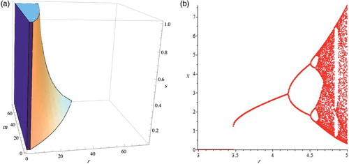
Figure 3. (a) We plot u(r, m, s)<2 represented by the region inside the above solid and (b) bifurcation diagram.

3. The hierarchical model

We consider the following Ricker-type [21] two-species hierarchical competition model with the Allee effect:

$\begin{array}{rl}{x}_{t+1}& =x_t{\mathrm{e}}^{r_1-x_t-m_1/(1+s_1{x}_t)},\\ y_{t+1}& =y_t{\mathrm{e}}^{r_2-y_t-b{x}_t-m_2/(1+s_2{y}_t),}\end{array}$

This model can be written in the general form

$\begin{array}{rl}{x}_{t+1}& =f_1(x_t)I_1(x_t)=f(x_t).\\ y_{t+1}& =f_2(x_t,y_t)I_2(y_t)=g(x_t,y_t),\end{array}$

where f₁(x) and f₂(x, y) represent the negative density dependence factors and I₁(x) and I₂(y) represent the positive density dependence caused by the strong Allee effects. The terms $I_1(x)={\mathrm{e}}^{-m_1/(1+s_1{x}_t)}$ and $I_2(y)={\mathrm{e}}^{-m_2/(1+s_2{y}_t)}$ represent the strong Allee effect caused by predator saturation of species x and y, respectively. Note that m_i represents the predation intensity, and s_i is a parameter proportional to the ‘handling time’, that is the duration of the capture and eating phase.

It should be noted that system (1) or (2) may be generated by the map $F:{\mathbb{R}}_{+}^2\to {\mathbb{R}}_{+}^2$ defined as $F(x,y)=(f(x),g(x,y))$. Such maps are called triangular maps [3] since their Jacobians are triangular matrices.

First we will find the boundary fixed points and determine their stability. There are five boundary fixed points: $(0,0),(A_1,0),(K_1,0),(0,A_2),(0,K_2)$, where A₁ and A₂ are the (single species) Allee threshold of species x and y, respectively, K₁ and K₂ are their carrying capacities, respectively. We have that $A_1=\frac{(r_1{s}_1-1)-\sqrt{(r_1{s}_1-1{)}^2-4s_1(m_1-r_1)}}{2s_1}$ and $K_1=\frac{(r_1{s}_1-1)+\sqrt{(r_1{s}_1-1{)}^2-4s_1(m_1-r_1)}}{2s_1}.$ Assumption (H) is now replaced with the following assumption: $(H_1):r_1{s}_1>1,m_1>r_1,(r_1{s}_1+1{)}^2>4s_1{m}_1.$

The second isocline equation is given by $r_2-y-bx-\frac{m_2}{1+s_{2}y}=0$ or

$x=\frac{1}{b}\left(r_2-y-\frac{m_2}{1+s_{2}y}\right).$

Putting x=0 in Equation (8) yields the equation

$s_2{y}^2-(r_2{s}_2-1)y+(m_2-r_2)=0.$

Thus $A_2=\frac{(r_2{s}_2-1)-\sqrt{(r_2{s}_2-1{)}^2-4s_2(m_2-r_2)}}{2s_2},$ and $K_2=\frac{(r_2{s}_2-1)+\sqrt{(r_2{s}_2-1{)}^2-4s_2(m_2-r_2)}}{2s_2}$

In order to ensure the presence of the (single species) Allee effect A₂, we make the following assumption: $(H_2):r_2{s}_2>1,m_2>r_2,(r_2{s}_2+1{)}^2>4s_2{m}_2.$

4. Stability of the boundary fixed points

In order to determine the local stability of the boundary fixed points, let us consider the Jacobian matrix $\mathrm{JF}(\genfrac{}{}{0ex}{}{x}{y})$ of our model. $\left(\begin{array}{cc}\left[1-x\left(1-\frac{m_1{s}_1}{(1+s_{1}x{)}^2}\right)\right]{\mathrm{e}}^{r_1-x-m_1/(1+s_{1}x)}& 0\\ -by{\mathrm{e}}^{r_2-y-bx-m_2/(1+s_{2}y)}& \left[1-y\left(1-\frac{m_2{s}_2}{(1+s_{2}y{)}^2}\right)\right]{\mathrm{e}}^{r_2-y-bx-m_2/(1+s_{2}y)}\end{array}\right).$ Now

$\mathrm{JF}\left(\begin{array}{c}0\\ 0\end{array}\right)=\left(\begin{array}{cc}{\mathrm{e}}^{r_1-m_1}& 0\\ 0& {\mathrm{e}}^{r_2-m_2}\end{array}\right).$

From Assumptions (H₁) and (H₂), the two eigenvalues of $\mathrm{JF}(\genfrac{}{}{0ex}{}{0}{0}),{\lambda }_1={\mathrm{e}}^{r_1-m_1}$ and ${\lambda }_2={\mathrm{e}}^{r_2-m_2}$ are less than one. Hence, (0, 0) is locally asymptotically stable (attractor). Note that if r₁≥m₁, species x would have no Allee effect as A₁ disappears for r₁>m₁ and merges with zero at r₁=m₁. Moreover, (0, 0) becomes a saddle.

Next we consider $\mathrm{JF}\left(\begin{array}{c}{A}_1\\ 0\end{array}\right)=\left(\begin{array}{cc}\left[1-A_1\left(1-\frac{m_1{s}_1}{(1+s_1{A}_1{)}^2}\right)\right]{\mathrm{e}}^{r_1-A_1-m_1/(1+s_1{A}_1)}& 0\\ 0& {\mathrm{e}}^{r_2-b{A}_1-m_2}\end{array}\right).$ By substituting from the first isocline equation $({\mathrm{e}}^{r_1-A_1-m_1/1+s_1{A}_1}=1)$, we have $\mathrm{JF}\left(\begin{array}{c}{A}_1\\ 0\end{array}\right)=\left(\begin{array}{cc}1-A_1\left(1-\frac{m_1{s}_1}{(1+s_1{A}_1{)}^2}\right)& 0\\ 0& {\mathrm{e}}^{r_2-m_2-b{A}_1}\end{array}\right).$

Clearly $0<{\lambda }_2={\mathrm{e}}^{r_2-m_2-b{A}_1}<1$ from Assumption H₂. From Assumption H₁, one may show that λ₁>1. Hence (A₁, 0) is a saddle with the unstable manifold lying on the x-axis and the stable manifold lying in the interior of ${\mathbb{R}}_{+}^2$.

Next we consider $\mathrm{JF}\left(\begin{array}{c}{K}_1\\ 0\end{array}\right)=\left(\begin{array}{cc}1-K_1\left(1-\frac{m_1{s}_1}{(1+s_1{K}_1{)}^2}\right)& 0\\ 0& {\mathrm{e}}^{r_2-m_2-b{K}_1}\end{array}\right).$

It may be easily shown that $0<{\lambda }_1=1-K_1(1-m_1{s}_1/(1+s_1{K}_1{)}^2)<1$. Under Equation (4) where K is replaced with K₂, $|{\lambda }_2|<1$. Hence (K₁, 0) is locally asymptotically stable with one stable manifold lying on the x-axis and the other stable manifold lying in the interior of ${\mathbb{R}}_{+}^2$.

Similarly, one may show that (0, A₂) is a saddle. Moreover (0, K₂) is locally asymptotically stable (attractor) under condition (4) where K is replaced by K₂.

A transcritical bifurcation occurs when $(r_1{s}_1+1{)}^2=4s_1{m}_1$, where $A_1=K_1=(r_1{s}_1-1)/2s_1$. Moreover, at this bifurcation λ₁=1 and the unstable manifold of A₁ merges with the stable manifold of K₁ to produce a semistable centre manifold on the x-axis. Note that when $(r_1{s}_1+1{)}^2<4s_1{m}_1$, there will be no Allee threshold point A₁ and species x has no Allee effect. The same scenario occurs for species y when $(r_2{s}_2+1{)}^2=4s_2{m}_2$. We now summarize our results in the following theorem.

Theorem 1

The following statements hold true under Assumptions H₁ and H₂.

• (i) The extinction equilibrium (0, 0) is locally asymptotically stable.

• (ii) The (single-species) Allee thresholds (A₁, 0) and (0, A₂) are saddle equilibria.

• (iii) The (single-species) carrying capacities (K₁, 0) and (0, K₂) are locally asymptotically stable under condition (4).

Moreover, if in Assumption H₁ we let $(r_1{s}_1+1{)}^2=4s_1{m}_1,$ then A₁ and K₁ merge to produce a semistable equilibrium on the x-axis. Analogous result holds for the species y.

5. Global dynamics of hierarchical models

In this section, we consider a planar triangular map $F:{\mathbb{R}}^2\to {\mathbb{R}}^2$ of the form $F(x,y)=(f(x),g(x,y))$. We assume that F is C¹ and all orbits are bounded. Our main goal here is to extend the following one-dimensional result to planar triangular maps.

Theorem 2 (Elaydi–Sacker)

Let $f:\mathbb{R}\to \mathbb{R}$ be a continuous map such that all orbits are bounded. Then every orbit converges to a fixed point if and only if there are no periodic orbits of prime period two.

In order to accomplish this task, we need the extension of Sharkovsky's Theorem [23] to triangular maps by Kloeden [16] to planar triangular maps.

Sharkovsky's ordering of the positive integers is as follows: $\begin{array}{rl}& 3▹5▹7▹\cdots \\ & 2\times 3▹2\times 5▹2\times 7▹\cdots \\ & ⋮\\ & 2^n\times 3▹2^n\times 5▹2^n\times 7▹\cdots \\ & ⋮\\ & 2^n▹2^{n-1}▹\cdots ▹2^1▹2^0.\end{array}$

Theorem 3 (Kloeden)

If a continuous triangular map F has a periodic orbit of prime period k, then it has periodic orbits of prime period r for all r such that $k▹r$.

Let $(x^{\ast },y^{\ast })$ be a fixed point of the map F. Then given an open neighbourhood U of $(x^{\ast },y^{\ast })$, the local stable manifold of $(x^{\ast },y^{\ast })$ in this neighbourhood is defined as $W_{\mathrm{loc}}^s((x^{\ast },y^{\ast }),U)=\{(z_1,z_2)\in U|$ there exists a sequence $\{z_1(-n),z_2(-n){\}}_{n=0}^{\mathrm{\infty }}\subset U$ with $(z_1^{(0)},z_2^{(0)})=(z_1,z_2)$ and $\underset{n\to \mathrm{\infty }}{lim}F(z_1(-n-1),z_2(-n-1))=(z_1(-n),z_2(-n))$ and $\underset{n\to \mathrm{\infty }}{lim}(z_1(-n),z_2(-n))=(x^{\ast },y^{\ast })$. The global unstable manifold is given by $W^u(x^{\ast },y^{\ast })=\bigcup _{n=0}^{\mathrm{\infty }}{F}^n(W_{\mathrm{loc}}^u(x^{\ast },y^{\ast })).$

Now for any (x₀, y₀) the omega limit set $\omega (x_0,y_0)=\{(u,\upsilon ):F^{n_k}(u,\upsilon )\to (x_0,y_0)$ as $k\to \mathrm{\infty }\}$.

We still need one more crucial result by Brunovsky and Polacik [6].

Theorem 4

Let $(x^{\ast },y^{\ast })$ be a fixed point of a C¹-triangular map F such that $(x^{\ast },y^{\ast })\in \omega (x_0,y_0),$ for some $(x_0,y_0)\in {\mathbb{R}}^2$. Assume further that $(x^{\ast },y^{\ast })$ is stable for $F{|}_{W_{\mathrm{loc}}^c(x^{\ast },y^{\ast })}$. Then either $\underset{n\to \mathrm{\infty }}{lim}{F}^n(x_0,y_0)=(x^{\ast },y^{\ast })$ or else $\omega (x_0,y_0)$ contains a point of $W_{\mathrm{loc}}^u(x^{\ast },y^{\ast })|\{(x^{\ast },y^{\ast })\}$.

Now we are ready to state our main result.

Theorem 5

Let $F:{\mathbb{R}}^2\to {\mathbb{R}}^2$ be a C¹-triangular map such that each fixed point $(x^{\ast },y^{\ast })$ of F is locally stable of $F{|}_{W_{\mathrm{loc}}^c(x^{\ast },y^{\ast })}$. Assume further that all orbits are bounded. Then every orbit in ℝ² converges to a fixed point if and only if there are no periodic orbits of prime period 2.

To facilitate the proof of this theorem, we first establish the following Lemma.

Lemma 6

If a triangle map F=(f, g) has no periodic orbits of prime period 2, then f has no periodic orbits of prime period greater than one, provided that all orbits are bounded.

Proof Assume that F has no periodic orbits of prime period 2. By Kloeden's theorem, F has no periodic orbits of any prime period greater than one. Now suppose that f has a periodic orbit $\{a_1,a_2\}$ of prime period 2. Then both a₁ and a₂ are fixed points of f². Next consider the map $g:{\mathbb{R}}^2\to \mathbb{R}$ and define two maps g₁ and $g_2:\mathbb{R}\to \mathbb{R}$ by $g_1(z)=g(a_1,z),g_2(z)=g(a_2,z)$. Let $\hat{g}=g_2\circ g_1$. By Theorem 2, either ĝ has a periodic orbit of prime period 2 or every orbit under ĝ converges to a fixed point of ĝ. In the latter case, we pick one of these fixed points denote it by $a_2^{\ast }$. Now $F(a_1,a_2^{\ast })=(a_2,g_1(a_2^{\ast })),F^2(a_1,a_2^{\ast })=(a_1,g_2(g_1(a_2^{\ast })))=(a_1,\hat{g}(a_2^{\ast }))=(a_1,a_2^{\ast })$. Thus $(a_1,a_2^{\ast })$ is a periodic orbit of prime period 2 under the map F, which is a contradiction.

On the other hand, if ĝ has a periodic orbit of prime period 2, then by the same argument, we can show that F has a periodic orbit of prime period 4. By Kloeden's theorem, F then would have a periodic orbit of prime period 2, which is a contradiction. This completes the proof of the Lemma.

Proof of Theorem 4 Let $(x_0,y_0)\in {\mathbb{R}}^2$. Since the map F=(f, g) is assumed to have no periodic orbits of prime period 2, it follows from Lemma 6, then the map f has no periodic orbits of prime period 2. Hence by Theorem 2, $\underset{n\to \mathrm{\infty }}{lim}{f}^n(x_0)=x^{\ast }$, where x* is a fixed point of  f. This implies that the omega limit set $\omega (x_0,y_0)$ is a subset of the fibre x=x*. Since the orbit O(x₀, y₀) is bounded, $\omega (x_0,y_0)\ne \phi$. Let $(x^{\ast },\hat{y})\in \omega (x_0,y_0)$. Define the map $\hat{g}:\mathbb{R}\to \mathbb{R}$ with $\hat{g}(z)=g(x^{\ast },z)$. Now if F has no periodic orbits of prime period 2, then so does ĝ. Hence by Theorem 2, $\underset{n\to \mathrm{\infty }}{lim}{\hat{g}}^n(\hat{y})=y^{\ast }$ for some fixed point y* of ĝ. Thus $F(x^{\ast },y^{\ast })=(x^{\ast },g(x^{\ast },y^{\ast }))=(x^{\ast },y^{\ast })$ and consequently $(x^{\ast },y^{\ast })$ is a fixed point of F. Since $\omega (x_0,y_0)$ is closed and invariant [11], it follows that $(x^{\ast },y^{\ast })\in \omega (x_0,y_0)$. By Theorem 5, either $\underset{n\to \mathrm{\infty }}{lim}{F}^n(x_0,y_0)=(x^{\ast },y^{\ast })$, and we are done, or there exists a point $(x^{\ast },\upsilon )\in \omega (x_0,y_0)\bigcap W_{\mathrm{loc}}^u(x^{\ast },y^{\ast })$. Note that $\underset{n\to \mathrm{\infty }}{lim}{F}^n(x^{\ast },\upsilon )=(x^{\ast },{\upsilon }^{\ast })$ for some fixed point $(x^{\ast },{\upsilon }^{\ast })$ of F. Hence $(x^{\ast },\upsilon )\in W_{\mathrm{loc}}^u(x^{\ast },{\upsilon }^{\ast })$. Moreover $(x^{\ast },{\upsilon }^{\ast })\in \omega (x_0,y_0)$. Now by Theorem 5, either $\underset{n\to \mathrm{\infty }}{lim}{F}^n(x_0,y_0)=(x^{\ast },{\upsilon }^{\ast })$ or $\omega (x_0,y_0)\bigcap W_{\mathrm{loc}}^u(x^{\ast },{\upsilon }^{\ast })|\{(x^{\ast },{\upsilon }^{\ast })\}\ne \phi$, which leads to a contradiction. This completes the proof of the theorem.

6. Global dynamics of the model

We begin by investigating the existence of the interior fixed points. The interior fixed points are the intersections of the isoclines x=A₁, x=K₁ and the curve

$x=\frac{1}{b}\left(r_2-y-\frac{m_2}{1+s_{2}y}\right).$

There are five scenarios:

• (i) No interior fixed points (Figure 4(a)).

• (ii) One interior fixed point $(A_1,y_{A_{10}})$ (Figure 4(d)).

• (iii) Two interior fixed points, $(A_1,y_{A_{11}}),(A_1,y_{A_{12}})$ (Figure 4(b)).

• (iv) Three interior fixed points $(A_1,y_{A_{11}}),(A_1,y_{A_{12}}),(K_1,y_{K_{10}})$ (Figure 4(e)).

• (v) Four interior fixed points $(A_1,y_{A_{11}}),(A_1,y_{A_{12}}),(K_1,y_{K_{11}}),$ $(K_1,y_{K_{12}})$ (Figure 4(c)).

Figure 4. (a) Zero interior fixed point, (b) two interior fixed points, (c) four interior fixed points, (d) one interior fixed point and (e) three interior fixed points.

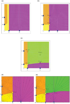
Remark In Figure 4(d) and 4(e) we plotted approximations of the phase space diagrams for one and three interior fixed points. This is due to the fact that obtaining an exact solution of x_max=A₁ or x_max=K₁ requires a certain degree of precision which is difficult to obtain by the computer.

6.1. The five scenarios

From Equation (11) we have $\frac{\mathrm{d}x}{\mathrm{d}y}=\frac{1}{b}\left(-1+\frac{m_2{s}_2}{(1+s_{2}y{)}^2}\right).$ The maximum value of x occurs when $\frac{\mathrm{d}x}{\mathrm{d}y}=0\text{or}(1+s_{2}y{)}^2=m_2{s}_2.$ Hence, $y=\frac{\sqrt{m_2{s}_2}-1}{s_2}.$ Substituting in x, yields

$x_{max}=\frac{1}{b}\left(r_2-\frac{2\sqrt{m_2{s}_2}-1}{s_2}\right).$

The location of x_max determines the number of interior fixed points. This is stated in the following Lemma.

Lemma 7

The following statements hold true.

• (i) If x_max<A₁, then there are no interior fixed points.

• (ii) If x_max=A₁, then we have one interior fixed point.

• (iii) If $A_1<x_{max}<K_1,$ then we have two interior fixed points.

• (iv) If x_max=K₁, then we have three interior fixed points.

• (v) If x_max>K₁, then we have four interior fixed points.

Proof The proof is straightforward and will be omitted.

Note that the y-component of the interior points $(A_1,y_{A_{10}})$ and $(K_1,y_{K_{10}})$ are given by $y_{A_{10}}=y_{K_{10}}=\frac{\sqrt{m_2{s}_2}-1}{s_2}.$

The other interior fixed points are obtained from Equation (4). For x=A₁ and x=K₁, we get $\begin{array}{rl}{y}_{A_{11},A_{12}}& =\frac{-b{A}_1{s}_2-1+r_2{s}_2\mp \sqrt{(b{A}_1{s}_2+1-r_2{s}_2{)}^2-4s_2(m_2-r_2+b{A}_1)}}{2s_2}.\\ y_{K_{11},K_{12}}& =\frac{-b{K}_1{s}_2-1+r_2{s}_2\mp \sqrt{(b{K}_1{s}_2+1-r_2{s}_2{)}^2-4s_2(m_2-r_2+b{K}_1)}}{2s_2}.\end{array}$ We now consider the local stability of the interior fixed points.

O.	No interior fixed point (Figure 4(a)). In this case, the extinction region (yellow) is unbounded and it lies between the line x=A1 and the stable manifold of (0, A2). The orange region is the exclusion region of y where every orbit converges to (0, K2), while the magenta region is the exclusion region of x where every orbit converges to (K1, 0).
I.	One interior fixed point $(A_1,y_{A_{10}})$ (Figure 4(d)). $\mathrm{JF}\left(\begin{array}{c}{A}_1\\ y_{A_{10}}\end{array}\right)=\left(\begin{array}{cc}1-A_1\left(1-\frac{m_1{s}_1}{(1+s_1{A}_1{)}^2}\right)& 0\\ -b{y}_{A_{10}}& 1-y_{A_{10}}\left(1-\frac{m_2{s}_2}{(1+s_2{y}_{A_{10}}{)}^2}\right)\end{array}\right).$ It is easy to show that $\begin{array}{rl}{\lambda }_1& =1-A_1\left(1-\frac{m_1{s}_1}{(1+s_1{A}_1{)}^2}\right)>1,\\ {\lambda }_2& =1-y_{A_{10}}\left(1-\frac{m_2{s}_2}{(1+s_2{y}_{A_{10}}{)}^2}\right)=1.\end{array}$ Here the centre manifold lies on the line x=A1. It is straightforward to show that this centre manifold is semistable. Here the extinction region (yellow) is bounded by the line x=A1 and the stable manifold of (0, A2). The exclusion region of y (orange) is bounded by the x=A1 and the stable manifold of (0, A2), while the exclusion region of x (magenta) is bounded by the line x=A1.
II.	Two interior fixed points (Figure 4(b)). In this scenario, the interior fixed point $(A_1,y_{A_{10}})$ splits into two interior fixed points $(A_1,y_{A_{11}})$ which is a repeller and $(A_1,y_{A_{12}})$ which is a saddle (Figure 4(b)). Note that for both points the Jacobian matrix has the eigenvalues $\begin{array}{rl}{\lambda }_1& =1-A_1\left(1-\frac{m_1{s}_1}{(1+s_1{A}_1{)}^2}\right)>1,\\ {\lambda }_2& =\left\{\begin{array}{ll}1-y_{A_{11}}\left(1-\frac{m_2{s}_2}{(1+s_2{y}_{A_{11}}{)}^2}\right)>1& \mathrm{for}\mathrm{JF}(A_1,y_{A_{11}}),\\ 1-y_{A_{12}}\left(1-\frac{m_2{s}_2}{(1+s_2{y}_{A_{12}}{)}^2}\right)<1& \mathrm{for}\mathrm{JF}(A_1,y_{A_{12}}).\end{array}\right.\end{array}$ The extinction region and the exclusion regions are the same as in the case of one interior fixed point.
III.	Three interior fixed points (Figure 4(e)). Here the dynamics of the interior fixed points $(A_1,y_{A_{11}})$ and $(A_1,y_{A_{12}})$ do not change. However, for the interior fixed point $(K_1,y_{K_{10}})$ the Jacobian matrix will have $0<{\lambda }_1<1$ and λ2=1. The centre manifold x=K1 is semistable as in the case of the interior fixed point $(A_1,y_{A_{10}})$. This is the first instance when we have a coexistence region. Here we have the extinction region (yellow), the exclusion region of y (orange), the exclusion region of x (magenta), and the coexistence region (green).
IV.	Four interior fixed points (Figure 4(c)). In this case the interior fixed point $(K_1,y_{K_{10}})$ splits into two interior fixed points $(K_1,y_{K_{11}})$ and $(K_1,y_{K_{12}})$. Note that $(K_1,y_{K_{11}})$ is a saddle and $(K_1,y_{K_{12}})$ is an attractor. The extinction region and the exclusion regions are the same as in the case of three interior fixed points.

Next we address the issue of the global dynamics of the system based on our main result, Theorem 5.

Theorem 8

Under Assumptions H₁ and H₂ and for the cases no interior fixed points, two interior fixed points, and four interior fixed points, every orbit in system (6) must converge to a fixed point.

Proof Note that the map $F=(f(x),g(x,y))$ in our model has no periodic orbits of prime period 2. For otherwise, $f(x)=x{\mathrm{e}}^{r_1-x-m_1/(1+s_{1}x)}$ would have a periodic orbit of prime period 2, which is false. Now $f(x)<x{\mathrm{e}}^{r_1-x}<{\mathrm{e}}^{r_1-1}$ and consequently, the maximum value of x_t is less than ${\mathrm{e}}^{r_1-1}$. Similarly, one may show that the maximum value of y_t is less than ${\mathrm{e}}^{r_2-1}$. Hence all orbits are bounded. Finally, since all fixed points are hyperbolic, Theorem 5 applies and thus every orbit must converge to a fixed point.

Remark As a consequence of Theorem 8, the global dynamics of the system is completely determined as depicted in Figure 4(a)–(e). Moreover, we conjecture that Figure 4(b) and 4(d) depict the global dynamics in the cases of one and three interior fixed points. We strongly believe that this conjecture is true based on the following explanation: one gets three interior fixed points from four fixed points through backward bifurcation when $(K_1,y_{K_{11}})$ and $(K_1,y_{K_{12}})$ merge leading to $(K_1,y_{K_{10}})$. This merger of a saddle point $(K_1,y_{K_{11}})$ and an attracting point $(K_1,y_{K_{12}})$ results into a semistable point $(K_1,y_{K_{10}})$. Similarly, we get a semistable point $(A_1,y_{A_{10}})$ by merging a repeller $(A_1,y_{A_{11}})$ and a saddle $(A_1,y_{A_{12}})$.

7. Conclusion

In this paper it is assumed that both species x and y possess the strong Allee effect. We found that when competition between species x and y is introduced an extinction region (yellow) always exists and hence a strong Allee effect persists in the competition model. In all scenarios, we have two exclusion regions: an exclusion region of species x (magenta) and an exclusion region of species y (orange). The only scenarios where we have a coexistence region of both species (green) are when we have three or four interior fixed points. From this we conclude that introducing competition is deleterious for both species that possess the strong Allee effect and survivability and persistence of both species is hard to achieve.

Acknowledgement

This work was supported by a grant from King Abdul Aziz University, Saudi Arabia.

References

- W.C. Allee, The Social Life of Animals, 3rd ed., William Heineman Ltd, London, 1941.
- L. Allen, J. Fagan, G. Hognas, and H. Fagerholm, Population extinction in discrete-time stochastic population models with an Allee effect, J. Differ. Equ. Appl. 11(4–5) (2005), pp. 273–293. doi: 10.1080/10236190412331335373
- E. Balreira, S. Elaydi, and R. Luis, Global dynamics of triangular maps, Nonlinear Anal., Theo., Meth. and Appl., Ser. A, 104 (2014), pp. 75–83. doi: 10.1016/j.na.2014.03.019
- J. Best and C. Castillo-Chavez, Hierarchical competition in discrete time models with dispersal, Fields Inst. Commun. 36 (2003), pp. 59–72.
- K.W. Blayneh, Hierarchical size-structured population model, Dyn. Syst. Appl. 9 (2000), pp. 527–539.
- P. Brunovsky and P. Polacik, On the structure of ω-limit sets of maps, Z. Angew. Math. Phys. 48 (1997), pp. 976–986.
- F. Courchamp, L. Berec, and J. Gascoigne, Allee Effects in Ecology and Conservation, Oxford University Press, Oxford, 2008.
- J.M. Cushing, The dynamics of hierarchical age-structural populations, J. Math. Biol. 32 (1994), pp. 705–729. doi: 10.1007/BF00163023
- J.M. Cushing, Backward bifurcations and strong Allee effects in matrix models for the dynamics of structural populations, J. Biol. Dyn. 8 (2014), pp. 57–73.
- J.M. Cushing and J. Hudson, Evolutionary dynamics and strong Allee effect, J. Biol. Dyn. 6(2) (2012), pp. 941–958. doi: 10.1080/17513758.2012.697196
- S. Elaydi, Discrete Chaos with Applications in Science and Engineering, 2nd ed., Chapman & CRC, Boca Raton, FL, 2008.
- S. Elaydi and R. Sacker, Basin of attraction of periodic orbits of maps on the real line, J. Differ. Equ. Appl. 10(10) (2004), pp. 881–888. doi: 10.1080/10236190410001731443
- S.M. Henson and J.M. Cushing, Hierarchical models of interspecific competition: scramble versus contest, J. Math. Biol. 34 (1996), pp. 755–772. doi: 10.1007/BF00161518
- S.R-J. Jang, Allee effects in a discrete-time host-parasitoid, J. Differ. Equ. Appl. 17 (2011), pp. 525–539. doi: 10.1080/10236190903146920
- A.P. Kinzig, S.A. Levin, J. Dushoff, and S. Pacak, Limiting similarity species packing and system stability for hierarchical competition colonization models, Am. Naturalist 153 (1999), pp. 371–383. doi: 10.1086/303182
- P. Kloeden, On Sharkovsky's cycle coexistence ordering, Bull. Aust. Math. Soc. 20 (1979), pp. 171–177. doi: 10.1017/S0004972700010819
- J. Li, B. Song, and X. Wang, An extended discrete Ricker population model with Allee effects, J. Diff. Equ. Appl. 13 (2007), pp. 309–321. doi: 10.1080/10236190601079191
- G. Livadiotis and S. Elaydi, General Allee effect in two-species population biology, J. Biol. Dyn. 6(2) (2012), pp. 959–973. doi: 10.1080/17513758.2012.700075
- G. Livadiotis, L. Assas, S. Elaydi, E. Kwessi, and D. Ribble, Competition models with Allee effects, J. Differ. Eq. Appl. to appear. 10.1080/10236198.2014.897341
- R. Luis, S. Elaydi, and H. Oliveira, Nonautonomous periodic systems with Allee effects, J. Differ. Eq. Appl. 16 (2010), pp. 1179–1196. doi: 10.1080/10236190902794951
- W.E. Ricker, Stock and recruitment, J. Fisheries Res. Board Canada 11(5) (1954), pp. 559–623. doi: 10.1139/f54-039
- S.J. Schreiber, Persistence for stochastic difference equations, a mini review, J. Differ. Equ. Appl. 3 (2012), pp. 1381–1403. doi: 10.1080/10236198.2011.628662
- A.N. Sharkovsky, Coexistence of cycles of a continuous map of the line into itself, Int. J. Bifurcation Chaos. 5 (1995), pp. 1263–1273. doi: 10.1142/S0218127495000934
- H.R. Thieme, T. Dhiraskodanon, Z. Han, and R. Trevino, Species decline and extinction: Synergy of infectious diseases and Allee effects, J. Biol. Dyn. 3 (2009), pp. 305–323. doi: 10.1080/17513750802376313