Full article: Modelling releases of sterile mosquitoes with different strategies

Formulae display: $MathJax Logo$ ?Mathematical formulae have been encoded as MathML and are displayed in this HTML version using MathJax in order to improve their display. Uncheck the box to turn MathJax off. This feature requires Javascript. Click on a formula to zoom.

Abstract

To prevent the transmissions of malaria, dengue fever, or other mosquito-borne diseases, one effective weapon is the sterile insect technique in which sterile mosquitoes are released to reduce or eradicate the wild mosquito population. To study the impact of the sterile insect technique on disease transmission, we formulate discrete-time mathematical models, based on difference equations, for the interactive dynamics of the wild and sterile mosquitoes, incorporating different strategies in releasing sterile mosquitoes. We investigate the model dynamics and compare the impact of the different release strategies. Numerical examples are given to demonstrate rich dynamical features of the models.

Keywords:

AMS Subject Classification:

1. Introduction

Mosquito-borne diseases, such as malaria and dengue fever, are a considerable public health concern worldwide. These diseases are transmitted between humans by blood-feeding mosquitoes. No vaccines are available and an effective way to prevent these mosquito-borne diseases is to control mosquitoes. Among the mosquitoes control measures, the sterile insect technique (SIT) has been applied to reduce or eradicate the wild mosquitoes. SIT is a method of biological control in which the natural reproductive process of the target population is disrupted. By chemical or physical methods, male mosquitoes are genetically modified to be sterile despite being sexually active. These sterile male mosquitoes are then released into the environment to mate with the wild mosquitoes. A wild female that mates with a sterile male will either not reproduce, or produce eggs that do not hatch. Repeated releases of genetically modified mosquitoes or the releases of a significantly large number of sterile mosquitoes may eventually wipe out a wild mosquito population, although it is, in practice, often more useful to consider controlling the population rather than eradicating it [Citation2,Citation8,Citation28].

The SIT is an effective weapon for fighting vector-borne diseases, and has shown promising results in laboratory studies. However, predicting the impact of releasing sterile mosquitoes into the field of wild mosquito populations is still a challenging task.

Mathematical models have proven useful in gaining insights into challenging questions in population dynamics and epidemiology. There are mathematical models in the literature formulated to study the interactive dynamics of mosquito populations or the control of mosquitoes [Citation3,Citation4,Citation6,Citation7,Citation9,Citation14,Citation15]. Models for vector-borne diseases, incorporating sterile mosquitoes, have also been formulated to investigate the disease transmission dynamics in [Citation11,Citation13,Citation27].

We focus, in this paper, on the dynamics of the interactive wild and sterile mosquitoes and explore the impact of different strategies of releasing sterile mosquitoes. Our approach is similar to that taken in [Citation9], although our model here is of discrete-time and based on difference equations. We consider homogeneous mosquito populations without distinguishing male or female individuals and assume that the mosquito dynamics follow the nonlinearity of Ricker-type in the absence of interactions. We consider the cases where the model equations for the interactive dynamics of the wild and sterile mosquitoes are based on the classical Ricker equation [Citation25], or the extended Ricker equation [Citation20] with Allee effects where we assume that mosquitoes have difficulty in finding mate at low population densities [Citation10]. We give general model descriptions in Section 2. In Section 3, we formulate a model for the case when sterile mosquitoes are released at a constant rate. We give a thorough analysis of the asymptotic dynamics of this model. In Section 4, we formulate a model for the case where when the number of released sterile mosquitoes is proportional to the wild mosquito population size. We assume difficulty in finding mates at low population densities, an assumption that introduces an Allee effect into the population dynamics. Mathematical analysis and numerical examples are presented that demonstrate the complexity of the model dynamics. To model a different releasing strategy, we assume, in Section 5, that the release is of Holling-II type, that is to say, the number of the sterile mosquito releases is proportional to the wild mosquito population size when the wild mosquito population size is small but saturates and approaches a constant as the wild mosquito population size is sufficiently large. We also give a complete mathematical analysis for the model's asymptotic dynamics. A brief discussion of our findings is given in Section 6, particularly with regard to the impact that the three different strategies have on mosquito control measures.

2. The model basis

We assume the mosquito population is homogeneous (by, e.g. not distinguishing their metamorphosis stages) and assume non-overlapping generations. In the absence of interaction with sterile mosquitoes, we let $w (n) = w_{n}$ be the wild mosquito population size at generation n, and the population dynamics be governed by the following equation: (1) $w_{n + 1} = C (w_{n}) a (w_{n}) w_{n} s (w_{n}),$ (1) where C is the number of matings per individual, a the number of offspring produced per mating, and $s (w_{n})$ the survival probability [Citation21–23]. We further assume a Ricker-type nonlinearity for the survival probability $s (w_{n}) = e^{- d - k w_{n}},$ where $\exp (- d)$ is the density-independent survival probability and k is the intraspecific competition coefficient (or carrying capacity parameter). We consider two different cases, without or with possible difficulty in finding mates at low population density.

Assume there is no difficulty in finding mates, and let the number of matings C and the number of offspring per mating be constants (density independent). If we re-label the product $C a \exp (- d)$ (which is the intrinsic population growth rate) as a, then the model equation (Equation1(1) $w_{n + 1} = C (w_{n}) a (w_{n}) w_{n} s (w_{n}),$ (1) ) becomes the classical Ricker equation (2) $w_{n + 1} = a w_{n} e^{- k w_{n}} .$ (2) As is well known, if $a < 1$ , the trivial fixed point $w = 0$ is the only fixed point and is globally asymptotically stable. If $a > 1$ , the trivial fixed point is unstable and there exists a unique positive fixed point $w = \ln a / k$ , which is globally asymptotically stable if $a < e^{2}$ , and is unstable if $a > e^{2}$ . A period-doubling bifurcation occurs as a increases.

To model the situation when mating difficulty arises in small population sizes, we assume $C (N_{n}) = c_{0} N_{n} / (1 + N_{n})$ , where $c_{0}$ is the maximum number of matings [Citation1,Citation10,Citation26]. By combining the coefficients as before, the model equation becomes (3) $w_{n + 1} = a \frac{w_{n}}{1 + w_{n}} w_{n} e^{- k w_{n}} .$ (3)

Equation (Equation3(3) $w_{n + 1} = a \frac{w_{n}}{1 + w_{n}} w_{n} e^{- k w_{n}} .$ (3) ) is similar to the extended Ricker equation studied in [Citation20]. The trivial fixed point $w = 0$ is always locally asymptotically stable. Let $w_{c} = \frac{\sqrt{k^{2} + 4 k} - k}{2 k} .$ We define the threshold value of the intrinsic growth rate of wild mosquitoes $a_{c}$ as (4) $a_{c} := \frac{2 + k + \sqrt{k^{2} + 4 k}}{2} \exp (\frac{\sqrt{k^{2} + 4 k} - k}{2})$ (4) and the threshold value for the stability $a_{s}$ as (5) $a_{s} := \frac{2 + k + \sqrt{k^{2} + 8 k + 4}}{2 - k + \sqrt{k^{2} + 8 k + 4}} \exp (\frac{2 - k + \sqrt{k^{2} + 8 k + 4}}{2}) .$ (5) We summarize the basic results for Equations (Equation2(2) $w_{n + 1} = a w_{n} e^{- k w_{n}} .$ (2) ) and (Equation3(3) $w_{n + 1} = a \frac{w_{n}}{1 + w_{n}} w_{n} e^{- k w_{n}} .$ (3) ) as follows.

Lemma 2.1.

If $a < 1$ in Equation (Equation2(2) $w_{n + 1} = a w_{n} e^{- k w_{n}} .$ (2) ) , the trivial solution $w = 0$ is the only fixed point and is globally asymptotically stable. If $a > 1,$ the trivial solution is unstable and there exists a unique positive fixed point which is globally asymptotically stable in the positive quadrant provided $a < e^{2}$ and is unstable provided $a > e^{2}$ . Equation (Equation3(3) $w_{n + 1} = a \frac{w_{n}}{1 + w_{n}} w_{n} e^{- k w_{n}} .$ (3) ) has no positive fixed point if $a < a_{c},$ one positive fixed point $w = w_{c}$ if $a = a_{c},$ which is unstable, and two positive fixed points $w_{1}^{*} < w_{c} < w_{2}^{*}$ if $a > a_{c},$ where $a_{c}$ is given in Equation (Equation4(4) $a_{c} := \frac{2 + k + \sqrt{k^{2} + 4 k}}{2} \exp (\frac{\sqrt{k^{2} + 4 k} - k}{2})$ (4) ) . Positive fixed point $w_{1}^{*}$ is always unstable, and $w_{2}^{*}$ is locally asymptotically stable if $a < a_{s},$ and is unstable if $a > a_{s},$ where $a_{s}$ is given in Equation (Equation5(5) $a_{s} := \frac{2 + k + \sqrt{k^{2} + 8 k + 4}}{2 - k + \sqrt{k^{2} + 8 k + 4}} \exp (\frac{2 - k + \sqrt{k^{2} + 8 k + 4}}{2}) .$ (5) ) .

Now suppose sterile mosquitoes are released into a wild mosquito population and we let $B_{n}$ be the number of the sterile mosquitoes released at time n. Since sterile mosquitoes do not reproduce, there is no maturation process from larvae to adults for sterile mosquitoes. Hence, the number of sterile mosquitoes at n is just the number of released sterile mosquitoes, and the size of total mosquitoes is $w_{n} + B_{n}$ at n. After the sterile mosquitoes are released, the mating interaction between the wild and sterile mosquitoes takes place. Similarly as in the homogeneous population models in [Citation17,Citation19], we assume harmonic means for matings, that is to say, the number of wild offspring produced per mating by wild mosquitoes is $\frac{a w_{n}}{w_{n} + B_{n}} .$

We assume that the complete life cycle of the mosquito occurs within one time unit of our model. While interspecific competition and predation are rather rare events and could be discounted as major causes of larval mortality, intraspecific competition could represent a major density-dependent source for the population dynamics, and hence the effect of crowding could be an important factor in the population dynamics of mosquitoes [Citation12,Citation16,Citation24]. We note that the intraspecific competition mainly takes place within the aquatic stages of mosquitoes and is due to resource and space limitations among larvae and pupa. For this reason, we assume that the density dependence is based only on larvae not adult numbers. Thus, we assume in our model that the probability of survival probability depends only on the wild mosquitoes and is independent of the released sterile mosquitoes [Citation5,Citation6,Citation18].

Therefore, if no difficulty in finding mates at low population densities exists, based on Equation (Equation2(2) $w_{n + 1} = a w_{n} e^{- k w_{n}} .$ (2) ) the interactive dynamics of the wild and sterile mosquitoes satisfy the following equation: (6) $w_{n + 1} = \frac{a w_{n}}{w_{n} + B_{n}} w_{n} e^{- k w_{n}} .$ (6) If there exists difficulty in finding mates, based on Equation (Equation3(3) $w_{n + 1} = a \frac{w_{n}}{1 + w_{n}} w_{n} e^{- k w_{n}} .$ (3) ) the interactive dynamics are governed by the following equation: (7) $w_{n + 1} = \frac{a w_{n}}{1 + w_{n} + B_{n}} w_{n} e^{- k w_{n}} .$ (7)

3. Constant releases

We assume sterile mosquitoes are constantly released in each generation so that $B_{n} := b > 0$ is a positive constant. With the constant releases, model (Equation6(6) $w_{n + 1} = \frac{a w_{n}}{w_{n} + B_{n}} w_{n} e^{- k w_{n}} .$ (6) ) becomes (8) $w_{n + 1} = \frac{a w_{n}}{w_{n} + b} w_{n} e^{- k w_{n}} .$ (8)

Clearly, the origin $w = 0$ is a fixed point and is always locally asymptotically stable. Moreover, if $a \leq 1$ , it follows from $w_{n + 1} < w_{n} e^{- k w_{n}}$ that there exists no positive fixed point and $w = 0$ is globally asymptotically stable.

Assume $a > 1$ and let $w_{n} := b y_{n}$ and $k_{1} = k b$ . Equation (Equation8(8) $w_{n + 1} = \frac{a w_{n}}{w_{n} + b} w_{n} e^{- k w_{n}} .$ (8) ) can be written as $y_{n + 1} = \frac{a y_{n}}{1 + y_{n}} y_{n} e^{- k_{1} y_{n}} .$ It follows from Lemma 2.1 that there exists a threshold of existence for positive fixed points as (9) $\begin{aligned} a_{c} & := \frac{2 + k_{1} + \sqrt{k_{1}^{2} + 4 k_{1}}}{2} \exp (\frac{\sqrt{k_{1}^{2} + 4 k_{1}} - k_{1}}{2}) \\ = \frac{2 + k b + \sqrt{(k b)^{2} + 4 k b}}{2} \exp (\frac{\sqrt{(k b)^{2} + 4 k b} - k b}{2}), \end{aligned}$ (9) such that there exist zero, one, or two positive fixed points if $a < a_{c}$ , $a = a_{c}$ , or $a > a_{c}$ , respectively.

Write $g (b) := \frac{\sqrt{(k b)^{2} + 4 k b} - k b}{2} .$ Then, $a_{c}$ in Equation (Equation9(9) $\begin{aligned} a_{c} & := \frac{2 + k_{1} + \sqrt{k_{1}^{2} + 4 k_{1}}}{2} \exp (\frac{\sqrt{k_{1}^{2} + 4 k_{1}} - k_{1}}{2}) \\ = \frac{2 + k b + \sqrt{(k b)^{2} + 4 k b}}{2} \exp (\frac{\sqrt{(k b)^{2} + 4 k b} - k b}{2}), \end{aligned}$ (9) ) can be defined as a function of b as (10) $a_{c} = H_{1} (b) := (1 + k b + g (b)) e^{g (b)} .$ (10) It follows from $g^{'} (b) = \frac{2 k}{\sqrt{(k b)^{2} + 4 k b} (2 + k b + \sqrt{(k b)^{2} + 4 k b})} > 0$ that $H_{1} (b)$ is a monotone increasing function. Hence for a given a, if we define the threshold value for the existence of positive fixed points to be $b_{c} = H_{1}^{- 1} (a),$ then $a < a_{c}$ , $a = a_{c}$ , or $a > a_{c}$ , if $b > b_{c}$ , $b = b_{c}$ , or $b < b_{c}$ , respectively. Therefore, $b_{c}$ establishes the threshold value for the existence of positive fixed points of Equation (Equation8(8) $w_{n + 1} = \frac{a w_{n}}{w_{n} + b} w_{n} e^{- k w_{n}} .$ (8) ).

For the stability of the positive fixed points of Equation (Equation8(8) $w_{n + 1} = \frac{a w_{n}}{w_{n} + b} w_{n} e^{- k w_{n}} .$ (8) ), it follows from Lemma 2.1 that the corresponding threshold value $a_{s}$ is $a_{s} := \frac{2 + k_{1} + \sqrt{k_{1}^{2} + 8 k_{1} + 4}}{2 - k_{1} + \sqrt{k_{1}^{2} + 8 k_{1} + 4}} \exp (\frac{2 - k_{1} + \sqrt{k_{1}^{2} + 8 k_{1} + 4}}{2}) .$ With $k_{1} = k b$ , the threshold value for stability of positive fixed points of Equation (Equation8(8) $w_{n + 1} = \frac{a w_{n}}{w_{n} + b} w_{n} e^{- k w_{n}} .$ (8) ) is (11) $a_{s} := \frac{2 + k b + \sqrt{k^{2} b^{2} + 8 k b + 4}}{2 - k b + \sqrt{k^{2} b^{2} + 8 k b + 4}} \exp (\frac{2 - k b + \sqrt{k^{2} b^{2} + 8 k b + 4}}{2}),$ (11) such that if there exist two positive fixed points $w_{1}^{*} < w_{2}^{*}$ , $w_{1}^{*}$ is always unstable, and $w_{2}^{*}$ is asymptotically stable provided $a < a_{s}$ , and unstable provided $a > a_{s}$ .

Write $p_{1} (b) := 2 + k b + D (b)$ , $p_{2} (b) := 2 - k b + D (b)$ , and $D (b) := \sqrt{k^{2} b^{2} + 8 k b + 4}$ . We write the right-hand side of Equation (Equation11(11) $a_{s} := \frac{2 + k b + \sqrt{k^{2} b^{2} + 8 k b + 4}}{2 - k b + \sqrt{k^{2} b^{2} + 8 k b + 4}} \exp (\frac{2 - k b + \sqrt{k^{2} b^{2} + 8 k b + 4}}{2}),$ (11) ) as function (12) $H_{2} (b) := \frac{p_{1} (b)}{p_{2} (b)} e^{p_{2} (b) / 2} .$ (12) Then, it follows from $H_{2}^{'} (b) = (\frac{p_{1}^{'} (b) p_{2} (b) - p_{1} (b) p_{2}^{'} (b)}{p_{2}^{2} (b)} + \frac{p_{1} (b) p_{2}^{'} (b)}{2 p_{2} (b)}) e^{p_{2} (b) / 2}$ that (13) $\begin{aligned} Δ (b) & := 2 p_{2}^{2} (b) e^{- p_{1} (b) / 2} H_{2}^{'} (b) = 2 p_{1}^{'} (b) p_{2} (b) - 2 p_{1} (b) p_{2}^{'} (b) + p_{1} (b) p_{2} (b) p_{2}^{'} (b) \\ = k (4 (2 + D (b)) - (2 + D (b))^{2} + k^{2} b^{2}) + D^{'} (b) ((2 + D (b))^{2} - k^{2} b^{2} - 4 k b) \\ = k (4 - D^{2} (b) + k^{2} b^{2}) + D^{'} (b) ((2 + D (b))^{2} - k^{2} b^{2} - 4 k b) . \end{aligned}$ (13) Substituting $D^{'} (b) = \frac{k^{2} b + 4 k}{D (b)}$ into Equation (Equation13(13) $\begin{aligned} Δ (b) & := 2 p_{2}^{2} (b) e^{- p_{1} (b) / 2} H_{2}^{'} (b) = 2 p_{1}^{'} (b) p_{2} (b) - 2 p_{1} (b) p_{2}^{'} (b) + p_{1} (b) p_{2} (b) p_{2}^{'} (b) \\ = k (4 (2 + D (b)) - (2 + D (b))^{2} + k^{2} b^{2}) + D^{'} (b) ((2 + D (b))^{2} - k^{2} b^{2} - 4 k b) \\ = k (4 - D^{2} (b) + k^{2} b^{2}) + D^{'} (b) ((2 + D (b))^{2} - k^{2} b^{2} - 4 k b) . \end{aligned}$ (13) ), we then find, after tedious algebra, $\begin{aligned} \frac{D (b)}{4 k} Δ (b) & = k^{2} b^{2} + 6 k b + 8 - b k D (b) + 4 D (b) \\ = \frac{4 k b (k^{2} b^{2} + 12 k b + 24) + 8}{k^{2} b^{2} + 6 k b + 8 + b k D (b)} + 4 D (b) > 0, \end{aligned}$ for $b \geq 0$ . Hence, $H_{2} (b)$ is a monotone increasing function of b. For a given a, let $b_{s} := H_{2}^{- 1} (a)$ . Then, if $b < b_{s}$ , $a_{s} < a$ , which implies the instability of $w_{2}^{*}$ and if $b > b_{s}$ , $a_{s} > a$ , which implies the asymptotic stability of $w_{2}^{*}$ .

In summary, we have the following results.

Theorem 3.1.

The trivial fixed point $w = 0$ of Equation (Equation8(8) $w_{n + 1} = \frac{a w_{n}}{w_{n} + b} w_{n} e^{- k w_{n}} .$ (8) ) is always locally asymptotically stable. For a given intrinsic growth parameter a, there exists a threshold release value of sterile mosquitoes $b_{c} = H_{1}^{- 1} (a)$ where $H_{1}$ is given in Equation (Equation10(10) $a_{c} = H_{1} (b) := (1 + k b + g (b)) e^{g (b)} .$ (10) ) . If the number of releases is greater than the threshold, that is, $b > b_{c},$ then $w = 0$ is the only fixed point that is globally asymptotically stable, and thus the wild mosquito population goes extinct regardless of the initial population size. If $b < b_{c},$ there exist two positive fixed points, $w_{1}^{*} < w_{c} = \frac{\sqrt{k^{2} b^{2} + 4 k b} - k b}{2 k} < w_{2}^{*} .$ Fixed point $w_{1}^{*}$ is always unstable. Fixed point $w_{2}^{*}$ is unstable if $b < b_{s},$ and is locally asymptotically stable if $b > b_{s},$ where $b_{s} = H_{2}^{- 1} (a)$ is the stability threshold with $H_{2} (b)$ given in Equation (Equation12(12) $H_{2} (b) := \frac{p_{1} (b)}{p_{2} (b)} e^{p_{2} (b) / 2} .$ (12) ) . Solutions approach either $w = 0$ or $w = w_{2}^{*}$ depending on their initial values.

Notice that positive fixed point $w_{2}^{*}$ is asymptotically stable for $b_{s} < b < b_{c}$ . As b decreases through $b_{s}$ , $w_{2}^{*}$ loses its stability and a stable 2-cycle bifurcates from it [Citation20]. If $b > 0$ continues decreasing, a backward period-doubling bifurcation occurs. We illustrate the results in Example 3.2.

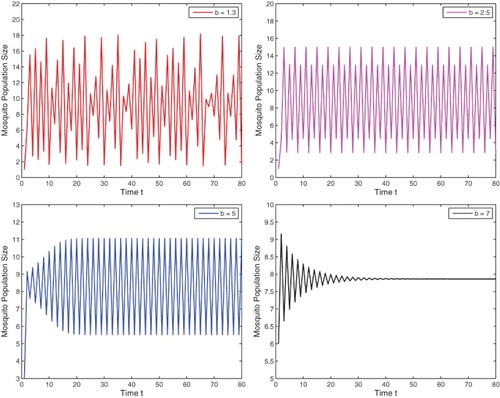
Example 3.1.

We choose the intrinsic growth rate $a = 20$ and $k = 0.3$ in Equation (Equation8(8) $w_{n + 1} = \frac{a w_{n}}{w_{n} + b} w_{n} e^{- k w_{n}} .$ (8) ). The threshold value for the existence of positive fixed points is $b_{c} = 21.4006$ and the threshold value for the stability is $b_{s} = 6.1465$ . Positive fixed point $w_{2}^{*}$ exists and is stable for $6.1465 < b < 21.4006$ . We choose four different b values for our numerical simulations. As $b = 1.3$ , the mosquito population exhibits chaotic behaviour. For b equals $2.5$ , 5, and then 7, a stable 4-cycle, a stable 2-cycle, and a stable 1-cycle (positive fixed point) are presented, respectively. All are shown in Figure , where the initial values are all $w = 1$ . Notice that with other small initial values, solutions will approach the origin $w = 0$ that are not shown here.

Figure 1. With parameters $a = 20$ and $k = 0.3$ as given in Example 3.2, four different values $b = 1.3, 2.5, 5, 7$ , are used. With the same initial value $w = 1$ , chaotic behaviour is exhibited in the upper left figure, and then stable 4-cycle, 2-cycle, and 1-cycle are presented in the upper right figure, the lower left and right figures, respectively.

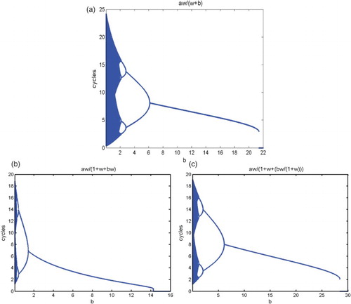
The bifurcation diagram is shown in Figure (a) and further discussion is given in Section 6.

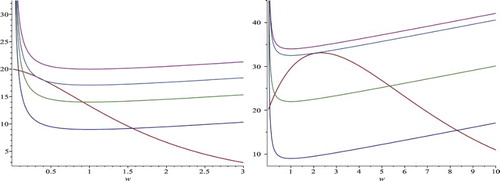
Figure 2. This is a schematic diagram to show the existence of positive fixed points. The figures on the left and right correspond to $k \geq 1$ and $k < 1$ , respectively. The intersection between the curve of $((1 + w)^{2} / w) + b$ and the curve of $a (1 + w) e^{- k w}$ gives a positive fixed point of Equation (Equation19(19) $w_{n + 1} = \frac{a w_{n}}{1 + w_{n} + B (w_{n})} w_{n} e^{- k w_{n}} = \frac{a w_{n} (1 + w_{n})}{(1 + w_{n})^{2} + b w_{n}} w_{n} e^{- k w_{n}} .$ (19) ). Keep the curve of $a (1 + w) e^{- k w}$ fixed. As parameter b increases gradually from zero to exceeding $b_{c}$ , the curve of $((1 + w)^{2} / w) + b$ moves up gradually. Accordingly, there exist two, one, or no intersections, and hence Equation (Equation19(19) $w_{n + 1} = \frac{a w_{n}}{1 + w_{n} + B (w_{n})} w_{n} e^{- k w_{n}} = \frac{a w_{n} (1 + w_{n})}{(1 + w_{n})^{2} + b w_{n}} w_{n} e^{- k w_{n}} .$ (19) ) has two, one, or no positive fixed points.

Figure 2. This is a schematic diagram to show the existence of positive fixed points. The figures on the left and right correspond to k≥1 and k<1, respectively. The intersection between the curve of ((1+w)2/w)+b and the curve of a(1+w)e−kw gives a positive fixed point of Equation (Equation19(19) wn+1=awn1+wn+B(wn)wne−kwn=awn(1+wn)(1+wn)2+bwnwne−kwn.(19) ). Keep the curve of a(1+w)e−kw fixed. As parameter b increases gradually from zero to exceeding bc, the curve of ((1+w)2/w)+b moves up gradually. Accordingly, there exist two, one, or no intersections, and hence Equation (Equation19(19) wn+1=awn1+wn+B(wn)wne−kwn=awn(1+wn)(1+wn)2+bwnwne−kwn.(19) ) has two, one, or no positive fixed points.

Notice that model (Equation8(8) $w_{n + 1} = \frac{a w_{n}}{w_{n} + b} w_{n} e^{- k w_{n}} .$ (8) ) has a density-dependent intrinsic growth rate $a w$ which is increasing for population density w near zero. Thus, this model has the so-called component Allee effect. Component Allee effects do not always lead to a strong Allee effect, that is, to two attractors one of which is extinction. However, they can in this model. More specifically, model (Equation8(8) $w_{n + 1} = \frac{a w_{n}}{w_{n} + b} w_{n} e^{- k w_{n}} .$ (8) ) has no Allee effects if there are no sterile mosquitoes, but the releasing strategy alone, not mating difficulty, can result in a strong Allee effect.

4. Releases proportional to the wild mosquito population size

To have a more economically effective strategy for releasing sterile mosquitoes in an area where the population size of wild mosquitoes is relatively small, instead of releasing sterile mosquitoes constantly in each generation, we may consider, by keeping close surveillance of the wild mosquitoes, letting the number of releases be proportional to the population size of the wild mosquitos. To model the strategy, we set $B = b w$ where b is a constant, and Equation (Equation3(3) $w_{n + 1} = a \frac{w_{n}}{1 + w_{n}} w_{n} e^{- k w_{n}} .$ (3) ) becomes (14) $w_{n + 1} = \frac{a w_{n}}{1 + (1 + b) w_{n}} w_{n} e^{- k w_{n}} .$ (14)

By letting $z_{n} = (1 + b) w_{n}$ , Equation (Equation14(14) $w_{n + 1} = \frac{a w_{n}}{1 + (1 + b) w_{n}} w_{n} e^{- k w_{n}} .$ (14) ) is translated into $z_{n + 1} = \frac{A z_{n}}{1 + z_{n}} z_{n} e^{- k_{1} z_{n}},$ where $A = a / (1 + b)$ and $k_{1} = k / (1 + b)$ .

It follows from Lemma 2.1 that there exists a threshold value for the existence of the positive fixed points of Equation (Equation14(14) $w_{n + 1} = \frac{a w_{n}}{1 + (1 + b) w_{n}} w_{n} e^{- k w_{n}} .$ (14) ) as (15) $A_{c} = \frac{2 + k_{1} + \sqrt{k_{1}^{2} + 4 k_{1}}}{2} \exp (\frac{\sqrt{k_{1}^{2} + 4 k_{1}} - k_{1}}{2}),$ (15) that is, in terms of a and k, Equation (Equation15(15) $A_{c} = \frac{2 + k_{1} + \sqrt{k_{1}^{2} + 4 k_{1}}}{2} \exp (\frac{\sqrt{k_{1}^{2} + 4 k_{1}} - k_{1}}{2}),$ (15) ) becomes $a_{c} = \frac{2 (1 + b) + k + \sqrt{k^{2} + 4 k (1 + b)}}{2} \exp (\frac{\sqrt{k^{2} + 4 k (1 + b)} - k}{2 (1 + b)}) := G_{1} (b),$ such that there exist no, one, or two positive fixed points if $a < a_{c}$ , $a = a_{c}$ , or $a > a_{c}$ , respectively.

By direct calculation, we have (16) $C (b) G_{1}^{'} (b) = 1 + \frac{Δ_{1}^{'}}{2} + \frac{1}{4} (k + 2 (1 + b) + Δ_{1}) (\frac{Δ_{1}^{'} (1 + b) - Δ_{1} + k}{(1 + b)^{2}}),$ (16) where $Δ_{1} (b) := \sqrt{k^{2} + 4 k (1 + b)}, C (b) := \exp (\frac{- Δ_{1} (b) + k}{2 (1 + b)}) .$

Substituting $Δ_{1}^{'} = 2 k / Δ_{1}$ into Equation (Equation16(16) $C (b) G_{1}^{'} (b) = 1 + \frac{Δ_{1}^{'}}{2} + \frac{1}{4} (k + 2 (1 + b) + Δ_{1}) (\frac{Δ_{1}^{'} (1 + b) - Δ_{1} + k}{(1 + b)^{2}}),$ (16) ) then yields $\begin{aligned} C (b) G_{1}^{'} (b) & = 1 + \frac{k}{Δ_{1}} + \frac{1}{4} (k + 2 (1 + b) + Δ_{1}) (\frac{2 k (1 + b) - Δ_{1}^{2} + k Δ_{1}}{Δ_{1} (1 + b)^{2}}) \\ = 1 + \frac{k}{Δ_{1}} + \frac{1}{4} (k + 2 (1 + b) + Δ_{1}) (\frac{k (- 2 (1 + b) - k + Δ_{1})}{Δ_{1} (1 + b)^{2}}) \\ = 1 + \frac{k}{Δ_{1}} + \frac{k}{4} (\frac{Δ_{1}^{2} - (2 (1 + b) + k)^{2}}{Δ_{1} (1 + b)^{2}}) \\ = 1 + \frac{k}{Δ_{1}} - \frac{k}{Δ_{1}} = 1. \end{aligned}$ Hence, $G_{1} (b)$ is a monotone increasing function. Define $b_{c} := G_{1}^{- 1} (a)$ for a given a. Then, Equation (Equation14(14) $w_{n + 1} = \frac{a w_{n}}{1 + (1 + b) w_{n}} w_{n} e^{- k w_{n}} .$ (14) ) has no, one, or two positive fixed points if $b > b_{c}$ , $b = b_{c}$ , or $b < b_{c}$ , respectively.

It follows from Lemma 2.1 again that there exists a threshold value for stability of the positive fixed points of Equation (Equation14(14) $w_{n + 1} = \frac{a w_{n}}{1 + (1 + b) w_{n}} w_{n} e^{- k w_{n}} .$ (14) ) (17) $A_{s} := \frac{2 + k_{1} + \sqrt{k_{1}^{2} + 8 k_{1} + 4}}{2 - k_{1} + \sqrt{k_{1}^{2} + 8 k_{1} + 4}} \exp (\frac{2 - k_{1} + \sqrt{k_{1}^{2} + 8 k_{1} + 4}}{2}),$ (17) that is, in terms of a and k, Equation (Equation17(17) $A_{s} := \frac{2 + k_{1} + \sqrt{k_{1}^{2} + 8 k_{1} + 4}}{2 - k_{1} + \sqrt{k_{1}^{2} + 8 k_{1} + 4}} \exp (\frac{2 - k_{1} + \sqrt{k_{1}^{2} + 8 k_{1} + 4}}{2}),$ (17) ) (18) $a_{s} = (1 + b) \frac{P_{1} (b)}{P_{2} (b)} \exp (\frac{P_{2} (b)}{2 (1 + b)}) := G_{2} (b),$ (18) where $Δ_{2} (b) := \sqrt{k^{2} + 8 k (1 + b) + 4 (1 + b)^{2}}$ and $P_{1} (b) := 2 (1 + b) + k + Δ_{2} (b), P_{2} (b) := 2 (1 + b) - k + Δ_{2} (b) .$

Similarly to showing the monotonicity of $H_{1} (b)$ in Section 3, we can show that $G_{2} (b)$ is a monotone increasing function and then the threshold value for stability in terms of b can be defined as $b_{s} := G_{2}^{- 1} (a)$ for a given a. In summary, we have the following results.

Theorem 4.1.

The trivial fixed point $w = 0$ for Equation (Equation14(14) $w_{n + 1} = \frac{a w_{n}}{1 + (1 + b) w_{n}} w_{n} e^{- k w_{n}} .$ (14) ) is always locally asymptotically stable. For a given intrinsic growth rate a, there exists a threshold release value of sterile mosquitoes $b_{c}$ given in Equation (Equation16(16) $C (b) G_{1}^{'} (b) = 1 + \frac{Δ_{1}^{'}}{2} + \frac{1}{4} (k + 2 (1 + b) + Δ_{1}) (\frac{Δ_{1}^{'} (1 + b) - Δ_{1} + k}{(1 + b)^{2}}),$ (16) ) such that if $b > b_{c},$ $w = 0$ is the only fixed point and is globally asymptotically stable. If $b < b_{c},$ there exist two positive fixed points, $w_{1}^{*} < w_{c} = \frac{\sqrt{k^{2} + 4 k} - k}{2 k (1 + b)} < w_{2}^{*} .$ Fixed point $w_{1}^{*}$ is always unstable. Fixed point $w_{2}^{*}$ is locally asymptotically stable if $b > b_{s},$ and is unstable if $b < b_{s},$ where $b_{s} = G_{2}^{- 1} (a)$ with $G_{2} (b)$ defined in Equation (Equation18(18) $a_{s} = (1 + b) \frac{P_{1} (b)}{P_{2} (b)} \exp (\frac{P_{2} (b)}{2 (1 + b)}) := G_{2} (b),$ (18) ) .

With the same parameters $a = 20$ and $k = 0.3$ as in Example 3.2, the threshold values are $b_{c} = 14.2543$ and $b_{s} = 1.4108$ , respectively. A backward period-doubling bifurcation occurs as b decreases as shown in Figure (b) in Section 6.

5. Proportional releases with saturation

The strategy of proportional releases introduced in Section 4, compared to the constant releases, may have an advantage when the size of the wild mosquito population is small since the size of releases is also small. However, when the wild mosquito population size is large, the release size should presumably also be large, which may exceed our affordability. We propose a new strategy in which the number of sterile mosquito releases is proportional to the wild mosquito population size when it is small, but saturates and approaches a constant when the wild mosquito population size increases. To this end, we let number the releases be of Holling-II type with the form of $B (w) = b w / (1 + w)$ . The interactive dynamics, based on Equation (Equation7(7) $w_{n + 1} = \frac{a w_{n}}{1 + w_{n} + B_{n}} w_{n} e^{- k w_{n}} .$ (7) ), are governed by the following equation: (19) $w_{n + 1} = \frac{a w_{n}}{1 + w_{n} + B (w_{n})} w_{n} e^{- k w_{n}} = \frac{a w_{n} (1 + w_{n})}{(1 + w_{n})^{2} + b w_{n}} w_{n} e^{- k w_{n}} .$ (19)

Again, $w = 0$ is a trivial fixed point of Equation (Equation19(19) $w_{n + 1} = \frac{a w_{n}}{1 + w_{n} + B (w_{n})} w_{n} e^{- k w_{n}} = \frac{a w_{n} (1 + w_{n})}{(1 + w_{n})^{2} + b w_{n}} w_{n} e^{- k w_{n}} .$ (19) ) and is locally asymptotically stable. A positive fixed point then satisfies the following equation: (20) $F (w) := \frac{(1 + w)^{2} + b w}{w} = \frac{(1 + w)^{2}}{w} + b = a (1 + w) e^{- k w_{n}} := h (w) .$ (20)

First, it follows from (21) $h^{'} (w) = a (1 - k (1 + w)) e^{- k w}$ (21) that if $k \geq 1$ , $h (w)$ is monotone decreasing. Suppose $k < 1$ . Then (22) $h^{'} (w) \{\begin{cases} > 0 & if x < \frac{1 - k}{k}, \\ < 0 & if x > \frac{1 - k}{k}, \end{cases}$ (22) and (23) $h^{″} (w) = a k (2 - k (1 + w)) e^{- k w} \{\begin{cases} < 0 & if w < \frac{2 - k}{k}, \\ > 0 & if w > \frac{2 - k}{k} . \end{cases}$ (23)

Then, it follows from $F^{'} (w) = 1 - \frac{1}{w^{2}} and F^{″} (w) = \frac{2}{w^{3}},$ for all $w > 0$ , that $F (w)$ has a minimum value at $w = 1$ and the curve is concave up. Then for either $k \geq 1$ where $h (w)$ is monotone decreasing as shown in Equation (Equation21(21) $h^{'} (w) = a (1 - k (1 + w)) e^{- k w}$ (21) ), or $k < 1$ where $h (w)$ is concave dawn as confirmed in Equations (Equation22(22) $h^{'} (w) \{\begin{cases} > 0 & if x < \frac{1 - k}{k}, \\ < 0 & if x > \frac{1 - k}{k}, \end{cases}$ (22) ) and (Equation23(23) $h^{″} (w) = a k (2 - k (1 + w)) e^{- k w} \{\begin{cases} < 0 & if w < \frac{2 - k}{k}, \\ > 0 & if w > \frac{2 - k}{k} . \end{cases}$ (23) ) that the two curves have two intersections, one intersection, or no intersection as b increases. A schematic diagram is shown in Figure , where the figures on the left and right correspond to $k \geq 1$ and $k < 1$ , respectively.

Figure 3. The model equation for the upper figure (a) is (Equation8(8) $w_{n + 1} = \frac{a w_{n}}{w_{n} + b} w_{n} e^{- k w_{n}} .$ (8) ) with the constant releases. The lower two figures (b) on the left and (c) on the right are based on equation (Equation14(14) $w_{n + 1} = \frac{a w_{n}}{1 + (1 + b) w_{n}} w_{n} e^{- k w_{n}} .$ (14) ) where the number of releases is proportional to the wild mosquito population size, and Equation (Equation19(19) $w_{n + 1} = \frac{a w_{n}}{1 + w_{n} + B (w_{n})} w_{n} e^{- k w_{n}} = \frac{a w_{n} (1 + w_{n})}{(1 + w_{n})^{2} + b w_{n}} w_{n} e^{- k w_{n}} .$ (19) ) where the number of releases is proportional to the wild mosquito population size plus the saturation, respectively. We fix the same parameters $a = 20$ and $k = 0.3$ , and use b as the bifurcation parameter. For $b_{s} < b < b_{c}$ , there exists a unique positive fixed point. As b decreases, backward period-doubling bifurcations occur for all of the model equations. Notice, in all of the figures, $b_{s}$ corresponds to the b point where there exists two fixed points on the left but only one on the right. The threshold value $b_{c}$ corresponds to the b value where there is a positive fixed on the left and no positive fixed point on the right.

Figure 3. The model equation for the upper figure (a) is (Equation8(8) wn+1=awnwn+bwne−kwn.(8) ) with the constant releases. The lower two figures (b) on the left and (c) on the right are based on equation (Equation14(14) wn+1=awn1+(1+b)wnwne−kwn.(14) ) where the number of releases is proportional to the wild mosquito population size, and Equation (Equation19(19) wn+1=awn1+wn+B(wn)wne−kwn=awn(1+wn)(1+wn)2+bwnwne−kwn.(19) ) where the number of releases is proportional to the wild mosquito population size plus the saturation, respectively. We fix the same parameters a=20 and k=0.3, and use b as the bifurcation parameter. For bs<b<bc, there exists a unique positive fixed point. As b decreases, backward period-doubling bifurcations occur for all of the model equations. Notice, in all of the figures, bs corresponds to the b point where there exists two fixed points on the left but only one on the right. The threshold value bc corresponds to the b value where there is a positive fixed on the left and no positive fixed point on the right.

Now, we determine the threshold value $b_{c}$ for the existence of positive fixed points as follows. With parameter $b = b_{c}$ , the two curves are tangent to each other at the critical point $w_{c}$ . Thus, they satisfy the two equations $F = h$ and $F^{'} = h^{'}$ , that is, (24) $\begin{aligned} \frac{(1 + w_{c})^{2}}{w_{c}} + b_{c} & = a (1 + w_{c}) e^{- k w_{c}}, \\ 1 - \frac{1}{w_{c}^{2}} & = a (1 - k (1 + w_{c})) e^{- k w_{c}}, \end{aligned}$ (24)

which leads to

(25) $b_{c} := \frac{(1 + w_{c})^{2} (1 - k w_{c} (1 + w_{c}))}{w_{c}^{2} (k (1 + w_{c}) - 1)} .$ (25) Substituting $b_{c}$ into (24a), we obtain (26) $1 - w_{c}^{2} = a w_{c}^{2} (k (1 + w_{c}) - 1) e^{- k w_{c}} .$ (26)

In summary, we have the following existence results for the positive fixed points.

Theorem 5.1.

Equation (Equation19(19) $w_{n + 1} = \frac{a w_{n}}{1 + w_{n} + B (w_{n})} w_{n} e^{- k w_{n}} = \frac{a w_{n} (1 + w_{n})}{(1 + w_{n})^{2} + b w_{n}} w_{n} e^{- k w_{n}} .$ (19) ) has no, one, or two positive fixed points if $b > b_{c},$ $b = b_{c},$ or $b < b_{c},$ respectively, where $b_{c}$ is defined in Equation (Equation25(25) $b_{c} := \frac{(1 + w_{c})^{2} (1 - k w_{c} (1 + w_{c}))}{w_{c}^{2} (k (1 + w_{c}) - 1)} .$ (25) ) with $w_{c}$ satisfying Equation (Equation26(26) $1 - w_{c}^{2} = a w_{c}^{2} (k (1 + w_{c}) - 1) e^{- k w_{c}} .$ (26) ) .

We next investigate the stability of the positive fixed points.

At a fixed point w, the derivative of the right-hand side of Equation (Equation19(19) $w_{n + 1} = \frac{a w_{n}}{1 + w_{n} + B (w_{n})} w_{n} e^{- k w_{n}} = \frac{a w_{n} (1 + w_{n})}{(1 + w_{n})^{2} + b w_{n}} w_{n} e^{- k w_{n}} .$ (19) ), denoted by $J_{2} (w)$ , equals $J_{2} (w) = 1 + Q (w)$ where (27) $\begin{aligned} Q (w) & := \frac{(1 + w)^{2} + b w^{2}}{((1 + w)^{2} + b w)^{2}} a w e^{- k w} - k w \\ = \frac{(1 + w)^{2} + b w^{2} - k w (1 + w) ((1 + w)^{2} + b w)}{(1 + w) ((1 + w)^{2} + b w)} \\ = \frac{(1 + w)^{2} (1 - k w (1 + w)) + b w^{2} (1 - k (1 + w))}{(1 + w) ((1 + w)^{2} + b w)} . \end{aligned}$ (27) Notice that $\begin{aligned} (1 + w) w^{2} (F^{'} (w) - h^{'} (w)) & = (w^{2} - 1) - w (1 - k (1 + w)) ((1 + w)^{2} + b e) \\ = - (1 + w)^{2} (1 - k w (1 + w)) - b w^{2} (1 - k (1 + w)) . \end{aligned}$ Hence $Q (w) = - \frac{w^{2} (F^{'} (w) - h^{'} (w))}{((1 + w)^{2} + b w)} .$ Then, it follows from $(F - h)^{'} (w_{1}^{*}) < 0$ that $w_{1}^{*}$ , if exists, is always unstable, and from $(F - h)^{'} (w_{2}^{*}) > 0$ that $w_{2}^{*}$ is asymptotically stable if $- Q (w_{2}^{*}) < 2$ .

We determine the stability threshold of Equation (Equation19(19) $w_{n + 1} = \frac{a w_{n}}{1 + w_{n} + B (w_{n})} w_{n} e^{- k w_{n}} = \frac{a w_{n} (1 + w_{n})}{(1 + w_{n})^{2} + b w_{n}} w_{n} e^{- k w_{n}} .$ (19) ) as follows. Solving $- Q (w_{s}) = 2$ in Equation (Equation27(27) $\begin{aligned} Q (w) & := \frac{(1 + w)^{2} + b w^{2}}{((1 + w)^{2} + b w)^{2}} a w e^{- k w} - k w \\ = \frac{(1 + w)^{2} + b w^{2} - k w (1 + w) ((1 + w)^{2} + b w)}{(1 + w) ((1 + w)^{2} + b w)} \\ = \frac{(1 + w)^{2} (1 - k w (1 + w)) + b w^{2} (1 - k (1 + w))}{(1 + w) ((1 + w)^{2} + b w)} . \end{aligned}$ (27) ), that is, $- (1 + w_{s})^{2} (1 - k w_{s} (1 + w_{s})) - b_{s} w_{s}^{2} (1 - k (1 + w_{s})) = 2 (1 + w_{s}) ((1 + w_{s})^{2} + b_{s} w_{s})$ for $b_{s}$ , we have (28) $b_{s} = \frac{(1 + w_{s})^{2} (1 + (1 + w_{s}) (2 - k w_{s}))}{w_{s} ((1 + w_{s}) (k w_{s} - 2) - w_{s})} .$ (28) Substituting it into Equation (Equation20(20) $F (w) := \frac{(1 + w)^{2} + b w}{w} = \frac{(1 + w)^{2}}{w} + b = a (1 + w) e^{- k w_{n}} := h (w) .$ (20) ), we have (29) $1 - w_{s}^{2} = a w_{s} ((k w_{s} - 2) (1 + w_{s}) - w_{s}) e^{- k w_{s}} .$ (29)

In summary, we have the following stability results for the positive fixed points.

Theorem 5.2.

If Equation (Equation19(19) $w_{n + 1} = \frac{a w_{n}}{1 + w_{n} + B (w_{n})} w_{n} e^{- k w_{n}} = \frac{a w_{n} (1 + w_{n})}{(1 + w_{n})^{2} + b w_{n}} w_{n} e^{- k w_{n}} .$ (19) ) has two positive fixed points, $w_{1}^{*} < w_{2}^{*},$ $w_{1}^{*}$ is always unstable. Positive fixed point $w_{2}^{*}$ is locally asymptotically stable provided $b > b_{s},$ and unstable provided $b < b_{s},$ where the stability threshold value $b_{s}$ is given in Equation (Equation28(28) $b_{s} = \frac{(1 + w_{s})^{2} (1 + (1 + w_{s}) (2 - k w_{s}))}{w_{s} ((1 + w_{s}) (k w_{s} - 2) - w_{s})} .$ (28) ) with $w_{s}$ the unique solution of Equation (Equation29(29) $1 - w_{s}^{2} = a w_{s} ((k w_{s} - 2) (1 + w_{s}) - w_{s}) e^{- k w_{s}} .$ (29) ) .

With the same parameters $a = 20$ and $k = 0.3$ , we have the existence threshold $b_{c} = 28.4446$ with $w_{c} = 2.0924$ , and the stability threshold $b_{s} = 6.1432$ with $w_{s} = 8.0150$ . A similar backward period-doubling bifurcation occurs as shown in Figure (c) in Section 6.

6. Concluding remarks

As one novel mosquito control measure, the sterile insect technique has been applied to reduce or eradicate wild mosquitoes which transmit mosquito-borne diseases. However, the interactive dynamics of wild and sterile mosquitoes are so complex that investigations and assessments of the impact of releasing sterile mosquitoes into the field are very challenging. To have a better understanding of the complexity of the interactive dynamics and provide useful guidance for good strategies in releasing sterile mosquitoes, we formulated mathematical models with different release functions $B (\cdot)$ of the sterile mosquitoes. Our discrete-time are based on the classical or the extended Ricker model in Equation (Equation6(6) $w_{n + 1} = \frac{a w_{n}}{w_{n} + B_{n}} w_{n} e^{- k w_{n}} .$ (6) ) or Equation (Equation7(7) $w_{n + 1} = \frac{a w_{n}}{1 + w_{n} + B_{n}} w_{n} e^{- k w_{n}} .$ (7) ), and the release function is assumed to be constant, proportional to w, or of Holling-II type, in model system (Equation8(8) $w_{n + 1} = \frac{a w_{n}}{w_{n} + b} w_{n} e^{- k w_{n}} .$ (8) ), (Equation14(14) $w_{n + 1} = \frac{a w_{n}}{1 + (1 + b) w_{n}} w_{n} e^{- k w_{n}} .$ (14) ), or (Equation19(19) $w_{n + 1} = \frac{a w_{n}}{1 + w_{n} + B (w_{n})} w_{n} e^{- k w_{n}} = \frac{a w_{n} (1 + w_{n})}{(1 + w_{n})^{2} + b w_{n}} w_{n} e^{- k w_{n}} .$ (19) ), respectively. In addition, in models (Equation14(14) $w_{n + 1} = \frac{a w_{n}}{1 + (1 + b) w_{n}} w_{n} e^{- k w_{n}} .$ (14) ) and (Equation19(19) $w_{n + 1} = \frac{a w_{n}}{1 + w_{n} + B (w_{n})} w_{n} e^{- k w_{n}} = \frac{a w_{n} (1 + w_{n})}{(1 + w_{n})^{2} + b w_{n}} w_{n} e^{- k w_{n}} .$ (19) ) we included a component Allee effect caused by mating difficulties at low population densities, an issue we deemed unnecessary for model (Equation8(8) $w_{n + 1} = \frac{a w_{n}}{w_{n} + b} w_{n} e^{- k w_{n}} .$ (8) ) because of the constant release of sterile mosquitoes.

We explored the existence of fixed points and their stability for all of these model equations. In particular, we established a threshold release value $b_{c}$ for the existence of positive fixed points such that when the release parameter b exceeds this existence threshold, no positive fixed points exist and hence the wild mosquito population goes to extinct. If the release parameter, on the other hand, is less than the threshold value $b_{c}$ , one or two positive fixed points exist. We also determined a threshold value $b_{s}$ for the stability of the positive fixed points such that if the release parameter is greater than this stability threshold, the positive fixed points are stable, and if the release parameter is less than the stability threshold, the positive fixed points are unstable and period-doubling bifurcations occur as the release parameter decreases. This is consistent with the nature of the Ricker nonlinearity in discrete models. We also notice that in the case when the number of releases is proportional to the wild mosquito population size and no mating difficulties occur at low densities, the model dynamics are similar to the classical Ricker model where the wild population approaches the trivial fixed point or the unique positive fixed point globally. In the other cases, however, after necessary transformations, the model equations are similar to the extended Ricker model, and hence there exist two positive fixed points as $b < b_{c}$ although only one of the two is asymptotically stable.

The three releasing strategies have different impacts on the dynamical features of the wild population. To compare the impact from the three different strategies, we use the same parameters $a = 20$ and $k = 0.3$ , and list the thresholds $b_{c}$ and $b_{s}$ for these models in Table , and give their bifurcation diagrams in Figure .

Table 1. Summary table for the threshold release values.

Display Table

Similar to the results for continuous-time models studied in [Citation9], the constant release strategy seems to have an advantage compared to the proportional release strategy in that it can drive the wild mosquito population to extinction with the fixed number of released sterile mosquitoes slightly exceeding its threshold release value $b_{c}$ , whereas the necessary number of released sterile mosquitoes, depending in w, can be much larger for the latter strategy for w sufficiently large. Nevertheless, such a strategy may not be economically practical (considering the cost of making and releasing sterile mosquitoes) if the size of the wild mosquitoes becomes small since it constantly releases the sterile mosquitoes no matter what the size of the wild mosquito population is. If we compare the two strategies with $B (w) = b w$ and $B (w) = b w / (1 + w)$ , while it follows from Figure that the threshold release value $b_{c}$ for the former is smaller than the latter, we notice that $b w / (1 + w)$ is much smaller than bw for large mosquito population sizes w. Overall, it seems that the strategy with $B (w) = b w / (1 + w)$ might be the more practical one.

Finally, we would like to point out that while we have realistically assumed that density dependence is based on larval or the aquatic stages of mosquitoes, our models do not distinguish different metamorphic stages. More accurate investigations of the impact of SIT on the transmission of the mosquito-borne diseases would be based on stage-structured population dynamics models.

Acknowledgments

The authors thank Dr Jim Cushing and an anonymous reviewer for their careful reading and valuable comments and suggestions.

Funding

This research was supported partially by US National Science Foundation grant DMS-1118150. A part of the work was performed while Zhiling Yuan was vising the University of Alabama in Huntsville.

References

Allee W.C., The Social Life of Animals, 2nd ed., Beacon Press, Boston, MA, 1958.
Google Scholar
Alphey L., Benedict M., Bellini R., Clark G.G., Dame D.A., Service M.W., and Dobson S.L., Sterile-insect methods for control of mosquito-borne diseases: An analysis, Vector-Borne Zoonotic Dis. 10 (2010), pp. 295–311. doi: 10.1089/vbz.2009.0014
PubMed Web of Science ®Google Scholar
Barclay H.J., The sterile insect release method for species with two-stage life cycles, Res. Popul. Ecol. 21 (1980), pp. 165–180. doi: 10.1007/BF02513619
Google Scholar
Barclay H.J., Pest population stability under sterile releases, Res. Popul. Ecol. 24 (1982), pp. 405–416. doi: 10.1007/BF02515585
Google Scholar
Barclay H.J., Modeling incomplete sterility in a sterile release program: Interactions with other factors, Popul. Ecol. 43 (2001), pp. 197–206. doi: 10.1007/s10144-001-8183-7
Web of Science ®Google Scholar
Barclay H.J., Mathematical models for the use of sterile insects, in Sterile Insect Technique. Principles and Practice in Area-Wide Integrated Pest Management, V.A. Dyck, J. Hendrichs, and A.S. Robinson, eds., Springer, Heidelberg, 2005, pp. 147–174.
Google Scholar
Barclay H.J. and Mackuer M., The sterile insect release method for pest control: A density dependent model, Environ. Entomol. 9 (1980), pp. 810–817. doi: 10.1093/ee/9.6.810
Web of Science ®Google Scholar
Bartlett A.C. and Staten R.T., Sterile insect release method and other genetic control strategies. Radcliffe's IPM World Textbook, 1996, http://ipmworld.umn.edu/chapters/bartlett.htm.
Google Scholar
Cai L., Ai S., and Li J., Dynamics of mosquitoes populations with different strategies for releasing sterile mosquitoes, SIAM, J. Appl. Math. (to appear in 2014).
Web of Science ®Google Scholar
Dennis B., Allee effects: Population growth, critical density, and the chance of extinction, Nat. Resour. Model. 3 (1989), pp. 481–538.
Google Scholar
Dumont Y. and Tchuenche J.M., Mathematical studies on the sterile insect technique for the Chikungunya disease and Aedes albopictus, J. Math. Biol. 65 (2012), pp. 809–854. doi: 10.1007/s00285-011-0477-6
PubMed Web of Science ®Google Scholar
Dye C., Intraspecific competition amongst larval aedes aegypti: Food exploitation or chemical interference, Ecol. Entomol. 7 (1982), pp. 39–46. doi: 10.1111/j.1365-2311.1982.tb00642.x
Web of Science ®Google Scholar
Esteva L. and Yang H.M., Mathematical model to assess the control of Aedes aegypti mosquitoes by the sterile insect technique, Math. Biosci. 198 (2005), pp. 132–147. doi: 10.1016/j.mbs.2005.06.004
PubMed Web of Science ®Google Scholar
Fister K.R., McCarthy M.L., Oppenheimer S.F., and Collins C., Optimal control of insects through sterile insect release and habitat modification, Math. Biosci. 244 (2013), pp. 201–212. doi: 10.1016/j.mbs.2013.05.008
PubMed Web of Science ®Google Scholar
Floresa J.C., A mathematical model for wild and sterile species in competition: immigration, Physica A 328 (2003), pp. 214–224. doi: 10.1016/S0378-4371(03)00545-4
Web of Science ®Google Scholar
Gleiser R.M., Urrutia J., and Gorla D.E., Effects of crowding on populations of aedes albifasciatus larvae under laboratory conditions, Entomologia Exp. Applicata 95 (2000), pp. 135–140. doi: 10.1046/j.1570-7458.2000.00651.x
Web of Science ®Google Scholar
Li Jia, Simple mathematical models for interacting wild and transgenic mosquito populations, Math. Biosci. 189 (2004), pp. 39–59. doi: 10.1016/j.mbs.2004.01.001
PubMed Web of Science ®Google Scholar
Li Jia, Simple stage-structured models for wild and transgenic mosquito populations, J. Diff. Equ. Appl. 17 (2009), pp. 327–347. doi: 10.1080/10236190802566491
Web of Science ®Google Scholar
Li Jia, Modeling of mosquitoes with dominant or recessive transgenes and Allee effects, Math. Biosci. Eng. 7 (2010), pp. 101–123.
Web of Science ®Google Scholar
Li Jia, Song B., and Wang X., An extended Ricker population model with Allee effects, J. Diff. Equ. Appl. 13 (2007), pp. 309–321. doi: 10.1080/10236190601079191
Web of Science ®Google Scholar
May R.M., Theoretical Ecology: Principles and Applications, Saunders, Philadelphia, 1976.
Google Scholar
May R.M. and Oster G.F., Bifurcations and dynamic complexity in simple ecological models, Amer. Nat. 110 (1976), pp. 573–599. doi: 10.1086/283092
Web of Science ®Google Scholar
May R.M., Conway G.R., Hassell M.P., and Southwood T.R.E., Time delays, density-dependence and single-species oscillations, J. Animal Ecol. 43 (1974), pp. 747–770. doi: 10.2307/3535
Web of Science ®Google Scholar
Otero M., Solari H.G., and Schweigmann N., A stochastic population dynamics model for Aedes aegypti: formulation and application to a city with temperate climate, Bull. Math. Biol. 68 (2006), pp. 1945–1974. doi: 10.1007/s11538-006-9067-y
PubMed Web of Science ®Google Scholar
Ricker W.E., Stock and recruitment, J. Fish. Res. Board Canada 11 (1954), pp. 559–623. doi: 10.1139/f54-039
Google Scholar
Schreiber S.J., Allee effects, extinctions, and chaotic transients in simple population models, Theor. Popul. Biol. 64 (2003), pp. 201–209. doi: 10.1016/S0040-5809(03)00072-8
PubMed Web of Science ®Google Scholar
Thome R.C.A., Yang H.M., and Esteva L., Optimal control of Aedes aegypti mosquitoes by the sterile insect technique and insecticide, Math. Biosci. 223 (2010), pp. 12–23. doi: 10.1016/j.mbs.2009.08.009
PubMed Web of Science ®Google Scholar
Wikipedia, Sterile insect technique, 2013, http://en.wikipedia.org/wiki/Sterile_insect_technique.
Google Scholar

Modelling releases of sterile mosquitoes with different strategies

Abstract

1. Introduction

2. The model basis

3. Constant releases

4. Releases proportional to the wild mosquito population size

5. Proportional releases with saturation

6. Concluding remarks

Table 1. Summary table for the threshold release values.

Acknowledgments

Funding

References

Information for

Open access

Opportunities

Help and information

Modelling releases of sterile mosquitoes with different strategies

Abstract

1. Introduction

2. The model basis

3. Constant releases

4. Releases proportional to the wild mosquito population size

5. Proportional releases with saturation

6. Concluding remarks

Table 1. Summary table for the threshold release values.

Acknowledgments

Funding

References

Related research

To cite this article:

Download citation

Your download is now in progress and you may close this window

Login or register to access this feature

Information for

Open access

Opportunities

Help and information

Keep up to date