A discrete-time host–parasitoid model with an Allee effect

Abstract

We introduce a discrete-time host–parasitoid model with a strong Allee effect on the host. We adapt the Nicholson–Bailey model to have a positive density dependent factor due to the presence of an Allee effect, and a negative density dependence factor due to intraspecific competition. It is shown that there are two scenarios, the first with no interior fixed points and the second with one interior fixed point. In the first scenario, we show that either both host and parasitoid will go to extinction or there are two regions, an extinction region where both species go to extinction and an exclusion region in which the host survives and tends to its carrying capacity. In the second scenario, we show that either both host and parasitoid will go to extinction or there are two regions, an extinction region where both species go to extinction and a coexistence region where both species survive.

Keywords:

• Allee effect
• host
• parasitoid
• stability
• coexistence
• extinction

AMS Subject Classification:

• 39A11
• 92D25

1. Introduction

When investigating host–parasite systems, one usually refers to the standard Nicholson–Bailey model [38] (1) $H_{t+1}=r{H}_t{e}^{-\gamma P_t},P_{t+1}=s{H}_t(1-e^{-\gamma P_t}),$(1) where H_t and P_t denote the host and parasitoid populations, respectively, at the start of season t. Each host that survives to the end of the season produces r hosts next year. The parasitoids search randomly for hosts with a search parameter a and hence the probability that a single host escapes parasitism from a single parasitoid is $e^{-\gamma }$ and from P_t parasitoids is $e^{-\gamma P_t}$. Early on, it was realized that this model is not realistic and predicts that both host and parasitoid population sizes will oscillate erratically and eventually either both species go extinct or the parasitoid population goes extinct while the host population size explodes.

In 1975, Beddington et al. [5] proposed a new model that would stabilize the Nicholson–Bailey population dynamics. These authors observed that the main defect in the Nicholson–Bailey model is the assumption that the only regulation of the host population is by the parasitoid. To remedy this situation, they included in their model a density-dependent self-regulation by the prey. The new model is (2) $H_{t+1}=H_t{e}^{r(1-H_t/K)-\gamma P_t},P_{t+1}=s{H}_t(1-e^{-\gamma P_t}),$(2)

In the absence of the parasitoid, the equation of the host becomes the famous Ricker model [13]. Kapcak et al. [24] investigated model (2) but using different parameters γ₁ and γ₂ in the exponential functions in (2). Using new mathematical tools, the authors were able to establish a mathematical foundation for most of the results that, previously, were based on numerical simulations. It should be noted that a more general formulation of density dependence models was introduced by [34,35].

In this paper, we consider both parasitism and the strong Allee effect on the host. Several recent papers on this subject have appeared [3,7,8,12,19–21,23,25,37,39,47,48]. The Allee effect phenomenon was introduced by Warden Clyde Allee in 1931 [1] and was widely publicized by the recent book by Courchamp et al. [9]. Allee proposed that the per capita birth rate declines at low population densities (sizes). At the time, Allee's ideas were revolutionary since most of the biology literature was advocating the negative density dependence principle where higher population size (density) would limit the population growth. The subject stayed moribund until recent decades during which interest in the Allee effect has exploded. Mathematical modelling picked up momentum and we mention here a few papers in this direction [2,8,10,11,16,17,26,36,40, 43–45]. Note that in this paper we focus on the strong Allee effect, which means the existence of a ‘critical density’, below which population declines to extinction and above which it may increase [31]. This differs from the weak Allee effect, which refers to a population that lacks a ‘critical density’, but where, at lower densities, the population growth rate rises with increasing densities. Hereafter, we refer to the Allee effect with its strong definition.

Our modelling of the Allee effect on the host–parasitoid system begins with a single-species model with the Allee effect, which was introduced in [15], (3) $x_{t+1}=\frac{a{x}_t^2+r{x}_t}{1+x_t^2}.$(3)

The dynamics of this model is straightforward. There are three equilibrium points. The extinction fixed point 0 is an attractor, the Allee threshold A (the critical density) is a repeller, and the carrying capacity K is an attractor. The parameter r is the intrinsic growth rate when the population size is below A, and the parameter a is the difference between A and K. Due to the presence of the Allee effect, it is always assumed that 0 < r < 1.

To extend the notion of the Allee effect in multi-species models, Livadiotis and Elaydi [29] embarked on the endeavour of establishing the mathematical concepts and foundation of the phenomenon [4]. This was followed by the paper [33], which focused on extending Equation (3) to two-species model of the form (4) $x_{t+1}=\frac{a_1{x}_t^2+r_1{x}_t}{1+x_t^2+b_1{y}_t},y_{t+1}=\frac{a_2{y}_t^2+r_2{y}_t}{1+y_t^2+b_2{x}_t}.$(4)

In this paper, we adapt this idea to develop an extension of the Nicholson–Bailey model [38] to the setting of a host–parasitoid system with an Allee effect present in the dynamics of the host: (5) $H_{t+1}=\frac{a{H}_t^2+r{H}_t}{1+H_t^2}{e}^{-\gamma P_t},P_{t+1}=s{H}_t(1-e^{-\gamma P_t}).$(5)

2. The model

2.1. Construction of the model

A general formulation of the host–parasitoid system is the following [7,27]: (6) $H_{t+1}=g(H_t)\cdot p(P_t),P_{t+1}=s{H}_t\cdot [1-p(P_t)],$(6) where $g(H_t)=H_t\cdot u(H_t)$ defines the host dynamics in the absence of the parasitoid. Here, $u(H)$ denotes the per capita growth rate of the host. A typical method of modelling species suffering from strong Allee effect is via (7) $u(H_t)=u_0(H_t)\cdot \mathrm{I}(H_t),$(7) where the function $u_0(H)$ is host fitness in the absence of an Allee effect, and $\mathrm{I}(H)$ represents the Allee effect on the fitness of the host population [29,33].

The probability that a host escapes from parasitism is given by [38] (8) $p(P_t)=e^{-\gamma P_t}.$(8)

However, other formulations of this probability were also suggested and studied, for example, in [6]: (9) $p(P_t)=\frac{1}{{\gamma }^{-1}+P_t},$(9) or the more general expression by May [34] (10) $p(P_t)={\left(1+\frac{1}{\kappa }\cdot \gamma P_t\right)}^{-\kappa }.$(10)

May's probability model (10) lays the groundwork for the theoretical framework of the kappa distribution [30], which is based on the generalized background of non-extensive statistics (e.g. [46]; see also [28,32] and references therein). This framework uses a special way of deforming the exponential function, with respect to a critical quantity called the kappa index, κ, and is defined as (11) ${\exp }_{\kappa }(-x)={\left(1+\frac{1}{\kappa }\cdot x\right)}^{-\kappa },\mathrm{with}{\exp }_{\kappa \to \mathrm{\infty }}(-x)=e^{-x}.$(11)

Using the deformed exponential, Equation (10) may be written as (12) $p(P_t)={\exp }_{\kappa }(-\gamma P_t),$(12) with the quantity 1/κ characterizing a measure of how far is the population from the classical case (thermal equilibrium, Poisson process, etc.) [31].

In this paper, we study the model given by the planar map $F:{\mathrm{\Re }}_{+}^2\to {\mathrm{\Re }}_{+}^2,$ defined on the non-negative quadrant given by (13) $\begin{array}{r}F(H,P)\equiv [f_1(H,P),f_2(H,P)]\mathrm{with}{f}_1(H,P)\equiv \frac{a{H}^2+rH}{1+H^2}{e}^{-\gamma P},f_2(H,P)\equiv sH(1-e^{-\gamma P}).\end{array}$(13)

2.2. Characteristics of the model

2.2.1. Isoclines

The two isoclines of the system (13) are given by the following curves C₁: $H_{t+1}=H_t$ or $H=f_1(H,P)$, and C₂: $P_{t+1}=P_t$ or $P=f_2(H,P)$. Namely, (14) $\begin{array}{rl}(\mathrm{C}1)H& =f_1(H,P)\Rightarrow P_1(H)=\frac{1}{\gamma }\cdot \ln \left(\frac{aH+r}{1+H^2}\right),\end{array}$(14) (15) $\begin{array}{rl}(\mathrm{C}2)P& =f_2(H,P)\Rightarrow P_2(H)=sH(1-e^{-\gamma P})=-sH\cdot \frac{H^2-aH+(1-r)}{aH+r}.\end{array}$(15)

2.2.2. Jacobian matrix

The linearization of the F around an equilibrium point (H*, P*) gives (16) $F\left(\begin{array}{c}H\\ P\end{array}\right)\equiv \left(\begin{array}{c}{H}^{*}\\ P^{*}\end{array}\right)+\mathrm{JF}(H^{*},P^{*})\cdot \left(\begin{array}{c}{H}^{*}\\ P^{*}\end{array}\right)+h(H^{*},P^{*}),$(16) where h is the nonlinear part of the Taylor expansion; the Jacobian matrix associated with (16) is given by (17) $\mathrm{JF}(H,P)=\left[\begin{array}{cc}\left(2\cdot \frac{aH+r}{1+H^2}-r\right)\frac{e^{-\gamma P}}{1+H^2}& -\gamma H\cdot \frac{aH+r}{1+H^2}{e}^{-\gamma P}\\ s(1-e^{-\gamma P})& s\gamma H{e}^{-\gamma P}\end{array}\right].$(17)

(${\lambda }_1$ and ${\lambda }_2$ denote the eigenvalues of the Jacobian matrix JF.)

We now compute the Jacobian matrix at different equilibria points:

For equilibria points, Equation (17) becomes as follows:

At the origin O(0,0), (18) $\mathrm{JF}(0,0)=\left(\begin{array}{cc}r& 0\\ 0& 0\end{array}\right).$(18)

At a boundary equilibrium on the H-axis, not the origin, ($H^{*}\ne 0,P^{*}=0$), (19) $\mathrm{JF}(H^{*},0)=\left(\begin{array}{cc}\frac{2-r}{a{H}^{*}+r}& -\gamma H^{*}\\ 0& s\gamma H^{*}\end{array}\right).$(19)

At an interior equilibrium $(H^{*}\ne 0,P^{*}\ne 0)$, (20) $\mathrm{JF}(H^{*},P^{*})=\left[\begin{array}{cc}\frac{2e^{\gamma P^{*}}-r}{a{H}^{*}+r}& -\gamma H^{*}\\ s(1-e^{-\gamma P^{*}})& s\gamma H^{*}{e}^{-\gamma P^{*}}\end{array}\right],$(20) where we used the following relation taken from isocline C₁: (21) $\frac{a{H}^{*}+r}{1+H^{*2}}=e^{\gamma P^{*}}.$(21)

3. Local stability

In this section, we investigate the existence and stability of all the equilibria points. We first start with studying the boundary equilibria; then, we continue with the interior equilibria.

3.1. Boundary equilibria

There are three boundary equilibria, the origin O(0,0), and another two equilibria on the H-axis, that is, the Allee threshold A and the carrying capacity K of the host: (22) $H_{\pm }=\frac{1}{2}a\pm \sqrt{{\left(\frac{1}{2}a\right)}^2-(1-r)},A\equiv H_{-},K\equiv H_{+}.$(22)

Note that the Allee threshold A exists if and only if 0 < r < 1. Also, there are no boundary equilibria on the P-axis, other than the origin.

Standing Assumption: Henceforth, it is assumed throughout the paper that 0 < r < 1 [33].

For the stability of the origin O, we observe from (18) that ${\lambda }_1=r<1$ and ${\lambda }_2=0$ (superstable), and thus O is an attractor, which will be denoted by O(A). (Note that for r>1, O becomes a saddle point, and there is no strong Allee effect A, which gives rise to the weak Allee effect on the host [9,22,40].) For the stability of the Allee threshold A and carrying capacity K, we observe from (19) the eigenvalues (23) ${\lambda }_1=\frac{2-r}{a{H}_{*}+r},{\lambda }_2=s\gamma H^{*}.$(23)

It can be easily shown that ${\lambda }_1>1$ for $H^{*}=A$ (unstable) and ${\lambda }_1<1$ for $H^{*}=K$ (stable). However, the second eigenvalue ${\lambda }_2$ can be either larger or smaller than 1. The only restriction is that if ${\lambda }_2{|}_A>1$, then ${\lambda }_2{|}_K=s\gamma K>s\gamma A={\lambda }_2{|}_A>1$. Hence,

1. if $s\gamma A>1$, then ${\lambda }_2{|}_A>1$ and ${\lambda }_2{|}_K>1$. Because ${\lambda }_1{|}_A>1$, ${\lambda }_1{|}_K<1$, we conclude that A is a repeller and K is a saddle, symbolized by (A,0)(R) and (K,0)(S), respectively;

2. if $s\gamma A<1$, then ${\lambda }_2{|}_A<1$; ${\lambda }_2{|}_K$ can be either $>1$ or $<1$. Since ${\lambda }_1{|}_A>1$, ${\lambda }_1{|}_K<1$, we conclude that A is a saddle and K can be either a saddle (if $s\gamma K>1$) or an attractor (if $s\gamma K<1$), symbolized by (A,0)(S), and (K,0)(S) or (K,0)(A), respectively.

3.2. Coexistence equilibria

We now turn our attention to the coexistence equilibria that lie in the interior of the positive quadrant. Our first objective is to determine conditions under which interior equilibria exist and, when they do, how many there are. In fact, we will show that either there are no coexistence equilibria or there is only one coexistence equilibrium. We now summarize our results in Theorem 1 whose proof will be facilitated by four lemmas (Lemmas A1–A4) in Appendix.

Theorem 1

For system (13), there can be either zero or one interior equilibrium. The interior equilibrium, symbolized by $(H_I^{*},P_I^{*})$, exists only if $s\gamma A<1$ and $s\gamma K>1$.

1. If $s\gamma A>1$, then there are no interior equilibria. The stability of the boundary equilibria is (A,0)(R) and (K,0)(S).

2. If $s\gamma A<1$ and $s\gamma K<1$, then there are no interior equilibria. If $s\gamma A<1$ and $s\gamma K>1$, there is one interior equilibrium. The stability of the boundary equilibria is (A,0)(S) and (K,0)(A), or (A,0)(S) and (K,0)(S), respectively.

Proof.

It follows from Lemmas A1–A4.

Definition 1

The ‘reference point’ on the H-axis is defined by $H_{\mathrm{ref}}\equiv 1/(s\gamma )$. It is critical for the existence of the interior equilibria: if $H_{\mathrm{ref}}<A$ or $K<H_{\mathrm{ref}}$, then there are no interior equilibria points, but if $A<H_{\mathrm{ref}}<K$, then there is one interior equilibrium.

Theorem 2

The interior equilibrium is located between $H_{\mathrm{ref}}<H_I^{*}<K$.

Proof

To find the interior equilibrium point, we let $P_1(H_I^{*})=P_2(H_I^{*})$ in (A15). Let (24) $u\equiv \frac{a{H}_I^{*}+r}{1+H_I^{*2}},\mathrm{then}\gamma P_I^{*}=\ln u,\mathrm{and}s\gamma H_I^{*}=\frac{\ln u}{1-1/u}.$(24)

Hence, (25) $s\gamma H_I^{*}=\frac{\ln u(H_I^{*})}{1-1/u(H_I^{*})}.$(25)

Now the function $\ln u\cdot (1-1/u{)}^{-1}$ is monotonically increasing and, therefore, attains its minimum value at u=1. It follows that for u>1, $1<\ln u\cdot (1-1/u{)}^{-1}$. Then, from (25) we obtain $s\gamma H_I^{*}\ge 1$ or $1/s\gamma =H_{\mathrm{ref}}\le H_I^{*}$ with the equality holds at the boundary equilibrium A.

Lemma 1

If $det\mathrm{JF}(H_I^{*},P_I^{*})<1$, then $\mathrm{Tr}\mathrm{JF}(H_I^{*},P_I^{*})<det\mathrm{JF}(H_I^{*},P_I^{*})+1$.

Proof

We have (26) $\mathrm{Tr}\mathrm{JF}(H_I^{*},P_I^{*})=\mathrm{\Psi }+s\gamma H_I^{*}{e}^{-\gamma P_I^{*}},det\mathrm{JF}(H_I^{*},P_I^{*})=(\mathrm{\Psi }+e^{\gamma P_I^{*}}-1)\cdot s\gamma H_I^{*}{e}^{-\gamma P_I^{*}},$(26) where (27) $\mathrm{\Psi }\equiv \frac{2e^{\gamma P_I^{*}}-r}{a{H}_I^{*}+r}.$(27)

If $det\mathrm{JF}(H_I^{*},P_I^{*})<1$, then (28) $\mathrm{\Psi }<\frac{e^{\gamma P_I^{*}}}{s\gamma H_I^{*}}+1-e^{\gamma P_I^{*}}.$(28)

We define $u\equiv (a{H}_I^{*}+r)/(1+H{}_I^{*2})=e^{\gamma P_I^{*}}$ similar to (24). Hence, (29) $\mathrm{\Psi }<{\mathrm{V}}_1(u)\equiv (u-1)\cdot \left(\frac{1}{\ln u}-1\right).$(29)

On the other hand, if $\mathrm{Tr}\mathrm{JF}(H_I^{*},P_I^{*})<det\mathrm{JF}(H_I^{*},P_I^{*})+1$, then $\begin{array}{rl}& \mathrm{\Psi }+s\gamma H_I^{*}{e}^{-\gamma P_I^{*}}<(\mathrm{\Psi }+e^{\gamma P_I^{*}}-1)\cdot s\gamma H_I^{*}{e}^{-\gamma P_I^{*}}+1\Rightarrow \mathrm{\Psi }\cdot (1-s\gamma H_I^{*}{e}^{-\gamma P_I^{*}})\\ & <(e^{\gamma P^i}-2)\cdot s\gamma H^i{e}^{-\gamma P^i}+1,\end{array}$

that is, in terms of u, (30) $\begin{array}{rl}& \mathrm{\Psi }\cdot \left(1-\frac{\ln u}{u-1}\right)<1+(u-2)\cdot \frac{\ln u}{u-1},\\ \mathrm{hence},& \mathrm{\Psi }<{\mathrm{V}}_2(u)\equiv 1+\frac{1}{1/\ln u-1/(u-1)},\end{array}$(30) where we used the fact that $\ln u/(u-1)\le 1$. This is shown as follows: the function $\ln u/(u-1)$ is monotonically decreasing, thus, its maximum value is at u=1, $[\ln u/(u-1)]{|}_{u=1}=1\ge \ln u/(u-1)$. Hence, $det\mathrm{JF}(H_I^{*},P_I^{*})<1\Rightarrow \mathrm{\Psi }<{\mathrm{V}}_1(u)$, and $\mathrm{Tr}\mathrm{JF}(H_I^{*},P_I^{*})<det\mathrm{JF}(H_I^{*},P_I^{*})+1\Rightarrow \mathrm{\Psi }<{\mathrm{V}}_2(u)$. However, ${\mathrm{V}}_1(u)\le 1<3\le {\mathrm{V}}_2(u)$, $\mathrm{\forall }u\ge 1$. (Recall that u=1 applies for $P_I^{*}=0$, i.e. the interior equilibrium coincides with the boundary equilibria A and K.) Thus, if $\mathrm{\Psi }<{\mathrm{V}}_1(u)$, then $\mathrm{\Psi }<{\mathrm{V}}_1(u)<{\mathrm{V}}_2(u)$, or if $det\mathrm{JF}(H_I^{*},P_I^{*})<1$, then $\mathrm{Tr}\mathrm{JF}(H_I^{*},P_I^{*})<det\mathrm{JF}(H_I^{*},P_I^{*})+1$.

Theorem 3

For system (13), the interior equilibrium exists if and only if $A<H_{\mathrm{ref}}<K$. The point on the H-axis that maximizes the function u(H) is symbolized by H_c, and it is located at $A<H_{\mathrm{ref}}<H_{\mathrm{c}}<K$. If the interior equilibrium is stable, then $H_{\mathrm{ref}}<H_{\mathrm{c}}<H_I^{*}<K$.

Proof

If the interior equilibrium is stable, then $\mathrm{Tr}\mathrm{JF}(H_I^{*},P_I^{*})<det\mathrm{JF}(H_I^{*},P_I^{*})+1<2$, or, from Lemma 1 we have that $det\mathrm{JF}(H_I^{*},P_I^{*})<1$ is sufficient. This is equivalent to $\mathrm{\Psi }<{\mathrm{V}}_1(u)$; but ${\mathrm{V}}_1(u)\le 1$ (with the equal sign corresponding to u=1), thus,$\mathrm{\Psi }<1$, or (31) $\begin{array}{rl}\mathrm{\Psi }& \equiv \frac{2e^{\gamma P_I^{*}}-r}{a{H}_I^{*}+r}<1\Rightarrow e^{\gamma P_I^{*}}=\frac{a{H}_I^{*}+r}{1+H{{}_I^{*}}^2}<\frac{1}{2}a{H}_I^{*}+r\Rightarrow \frac{(1/2)a}{(1/2)a{H}_I^{*}+r}<H_I^{*},\\ \mathrm{that}\mathrm{is},H_{\mathrm{c}}& \equiv -\frac{r}{a}+\sqrt{{\left(\frac{r}{a}\right)}^2+1}<H_I^{*}.\end{array}$(31)

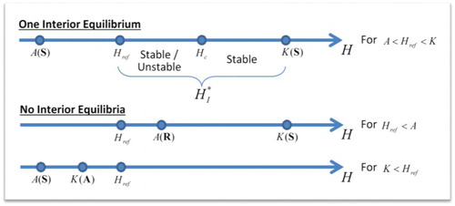
Figure 1 demonstrates the position of boundary and interior equilibria, and the conditions for their existence and stability.

Figure 1. Arrangement of the H-values that condition the existence and stability of boundary and interior equilibria: one interior equilibrium when (A,0)(S)<H_ref<(K,0)(S), and zero interior equilibria when H_ref<(A,0)(R)<(K,0)(S) or (A,0)(S)<(K,0)(A)<H_ref (S: Saddle, A: Attractor, R: Repeller).

Figure 2 helps to visualize the location of the interior equilibria with respect to the boundary equilibria A and K. In this figure, we plot several orbits of the phase-space portrait of the model (13). The interior equilibrium is parameterized by the argument u, (32) $s\gamma H_I^{*}(u)=\frac{\ln u}{1-1/u},\gamma P_I^{*}(u)=\ln u.$(32) All the possible values of u form the geometric locus of the interior equilibrium (black line) in Figure 2.

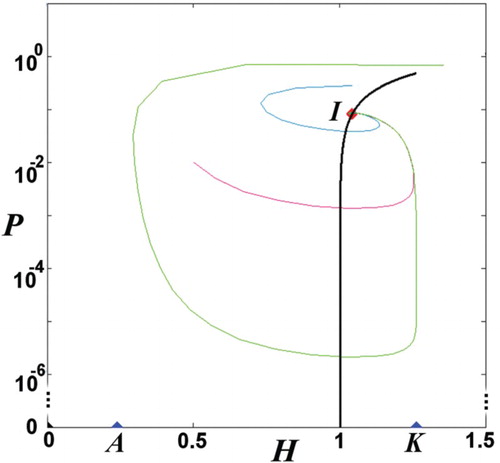
Figure 2. Phase-space portrait on a semi-log scale. (Namely, we plot (H,P) in a linear scale for H and logarithm scale for P, in order to show the variation of values of P over several orders of magnitude.) The boundary equilibria are located from both sides of the reference point $H_{\mathrm{ref}}=1/(s\gamma )=1$ (for sγ=1), so that $A<H_{\mathrm{ref}}<K$; hence, there exists one interior equilibrium $(H_I^{*},P_I^{*})$. The interior equilibrium is located between $H_{\mathrm{ref}}<H_I^{*}<K$ (Theorem 2) that can be also verified from the geometric locus of the interior equilibrium (black line).

Theorem 4

For system (13), the interior equilibrium does not exist if $a<1/(s\gamma )+(1-r)\cdot (s\gamma )$.

Proof

If $K<H_{\mathrm{ref}}$, then according to Theorem 3, the interior equilibrium does not exist. Substituting K from (22), we obtain $\frac{1}{2}a+\sqrt{{(\frac{1}{2}a)}^2-(1-r)}<1/(s\gamma )$ or $1/(s\gamma {)}^2-a/(s\gamma )+(1-r)>0$, which finally gives $a<1/(s\gamma )+(1-r)(s\gamma )$. Note that this must be true for any r, thus it can lead to a strongest condition for r=1, that is, $a<1/(s\gamma )$.

The region in the parameter space (a,r) that corresponds to $a<1/(s\gamma )+(1-r)(s\gamma )$ can be divided into two subregions $a<2/(s\gamma )$ and $a>2/(s\gamma )$. If $a<2/(s\gamma )$ then $K<H_{\mathrm{ref}}$, while if $a>2/(s\gamma )$ then $H_{\mathrm{ref}}<A$. The three curves in the parameter space (a,r), (i) $a=1/(s\gamma )+(1-r)(s\gamma )$, (ii) $a=2/(s\gamma )$, and (iii) $(\frac{1}{2}a{)}^2=(1-r)$ (that is the critical condition for the existence of the boundary equilibria A and K), intersect at the same point, $(a,r)=[2/(s\gamma ),1-1/(s\gamma {)}^2]$. This separates the regions of boundary but no interior equilibria into two subregions, corresponding to the two conditions $K<H_{\mathrm{ref}}$ and $H_{\mathrm{ref}}<A$. (For more details, see Figure 4(a).)

Note that the converse of the above statement may not hold.

Theorem 5

For system (13), the curve that corresponds to $det\mathrm{JF}(H_I^{*},P_I^{*})=1$ separates the cases of stable and unstable interior equilibrium, and it is given parametrically by $D=[a=D_a(u),r=D_r(u);1\le u;0<s\gamma <\mathrm{\infty }]$ (Figure 4).

Proof

The condition $det\mathrm{JF}(H_I^{*},P_I^{*})=1$ corresponds to $\mathrm{\Psi }={\mathrm{V}}_1(u)$, as concluded in Lemma 1, $\begin{array}{rl}\mathrm{\Psi }& \equiv \frac{2e^{\gamma P_I^{*}}-r}{a{H}_I^{*}+r}=\frac{2-r/u}{1+H_I^{*}{(u;s\gamma )}^2}={\mathrm{V}}_1(u),H_I^{*}(u;s\gamma )=\frac{1}{s\gamma }\cdot \frac{\ln u}{1-1/u},\\ {\mathrm{V}}_1(u)& =(u-1)\cdot \left(\frac{1}{\ln u}-1\right).\end{array}$

Solving in terms of r, we obtain (33a) $r(u;s\gamma )=2u-u(u-1)\left(\frac{1}{\ln u}-1\right)\left[1+\frac{1}{{(s\gamma )}^2}\cdot \frac{{\ln }^{2}u}{{(1-1/u)}^2}\right].$(33a)

Inverting the first part of (24) to express a in terms of u, we have $a(u;s\gamma )=\frac{u[1+H_I^{*}{(u;s\gamma )}^2]-r(u;s\gamma )}{H_I^{*}(u;s\gamma )},$ (33b) $\mathrm{or}a(u;s\gamma )=\frac{[(u-1)/\ln u+2-u]\cdot \{1+[1/(s\gamma ){]}^2{\ln }^{2}u/{(1-1/u)}^2\}-2}{[1/(s\gamma )]\cdot \ln u/(u-1)}.$(33b)

Hence, the function $D=[a=D_a(u),r=D_r(u);1\le u;0<s\gamma <\mathrm{\infty }]$ is given by (34) $\begin{array}{rl}{D}_a(u)& =\frac{[(u-1)/\ln u+2-u]\cdot \{1+[1/(s\gamma ){]}^2{\ln }^{2}u/{(1-1/u)}^2\}-2}{[1/(s\gamma )]\cdot \ln u/(u-1)},\\ D_r(u)& =2u-u(u-1)\left(\frac{1}{\ln u}-1\right)\left[1+\frac{1}{{(s\gamma )}^2}\cdot \frac{{\ln }^{2}u}{{(1-1/u)}^2}\right].\end{array}$(34)

The proof of the theorem is now complete.

Figure 3 depicts the function $D$ for several values of the parameter product s·γ.

Figure 3. Graphs of the function $D=[a(u),r(u);1\le u;0<s\gamma <\mathrm{\infty }]$, with a(u) and r(u) given by Equation (34), are depicted for various values of the parameter product s·γ, that is, <1 (blue dash), =1 (red solid), and >1 (green dash-dot). This function is the geometric locus of the parameters (a, r) that correspond to $det\mathrm{JF}(H_I^{*},P_I^{*})=1$ (for the map (13)). Note that the interior equilibrium does not exist for $a<1/(s\gamma )+(1-r)(s\gamma )$ (Theorem 4).

It is not a coincidence that all the previously shown stability equations and conditions include the product of the parameters s and γ, rather than each of them individually. Indeed, map (13) can be rewritten to the following tri-parametrical system without any loss of the complexity and dynamics, (35) ${\tilde{H}}_{t+1}=f_1({\tilde{H}}_t,{\tilde{P}}_t)\equiv {\tilde{H}}_t\frac{\tilde{a}{\tilde{H}}_t+r}{1+\beta {{\tilde{H}}_t}^2}{e}^{-{\tilde{P}}_t},{\tilde{P}}_{t+1}=f_2({\tilde{H}}_t,{\tilde{P}}_t)\equiv {\tilde{H}}_t(1-e^{-{\tilde{P}}_t}),$(35) where $\tilde{a}\equiv a/(s\gamma )$, $\beta \equiv (s\gamma {)}^{-2}$. Therefore, we use only the tri-parametrical (a,r) and s·γ to characterize the stability of the phase space.

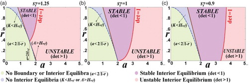
Figure 4 shows (i) the stability of the boundary equilibria, and (ii) the existence and stability of the interior equilibrium, in the parameter space (a,r) and for various of the parameter product $s\gamma$.

Figure 4. The parameter-space classification according to the existence and stability of the interior and boundary equilibria. (a) H_ref= 0.8 < 1 (s = 0.5,γ = 2.5); (b) H_ref= 1 (s = 0.5,γ = 2); (c) H_ref= 10/9>1 (s = 0.5,γ=1.8). (The symbol ‘det’ means $det\mathrm{JF}(H_I^{*},P_I^{*})$.)

Theorem 6

For system (13), the curve that corresponds to $det\mathrm{JF}(H_I^{*},P_I^{*})-\frac{1}{4}\mathrm{Tr}\mathrm{JF}(H_I^{*},P_I^{*}{)}^2=0$ separates the cases when a stable interior equilibrium has real eigenvalues with those when it has complex eigenvalues. This curve is given parametrically by $C=[a=c_a(u),r=c_r(u);1\le u;0<s\gamma <\mathrm{\infty }]$.

Proof

First we note that the element $det\mathrm{JF}(H_I^{*},P_I^{*})-\frac{1}{4}\mathrm{Tr}\mathrm{JF}(H_I^{*},P_I^{*}{)}^2$ is briefly symbolized by the operator $det-\frac{1}{4}{\mathrm{Tr}}^2$ acting on the Jacobian matrix, that is, $(det-\frac{1}{4}{\mathrm{Tr}}^2)\mathrm{JF}(H_I^{*},P_I^{*})$.

A stable interior equilibrium, I(A), can be an attractor for real or complex eigenvalues, corresponding to the conditions $(det-\frac{1}{4}{\mathrm{Tr}}^2)\mathrm{JF}(H_I^{*},P_I^{*})<0$ and $(det-\frac{1}{4}{\mathrm{Tr}}^2)\mathrm{JF}(H_I^{*},P_I^{*})>0$, respectively [14]. These two conditions separate the stable region into two sub-regions (not shown in figures), with their separatrix C expressed as follows. Given Equations (26) and (27), we obtain (36) $\mathrm{Tr}\mathrm{JF}(H_I^{*},P_I^{*})=\mathrm{\Psi }(u;s\gamma )+\frac{\ln u}{u-1},det\mathrm{JF}(H_I^{*},P_I^{*})=\left[\frac{\mathrm{\Psi }(u;s\gamma )}{u-1}+1\right]\cdot \ln u,$(36) where (37) $\mathrm{\Psi }(u;s\gamma )=\frac{2-r/u}{1+H_I^{*}{(u;s\gamma )}^2},H_I^{*}(u;s\gamma )=\frac{1}{s\gamma }\cdot \frac{\ln u}{1-1/u}.$(37)

Hence, the condition $(det-\frac{1}{4}{\mathrm{Tr}}^2)\mathrm{JF}(H_I^{*},P_I^{*})=0$ corresponds to the following curve of the parameter space (a,r), $C=[a=C_a(u),r=C_r(u);1\le u;0<s\gamma <\mathrm{\infty }]$, with (38) $\begin{array}{rl}{C}_a(u)& =\frac{\left[1+\ln u/(u-1)+2\sqrt{\ln u}\right]\cdot \{1+[1/(s\gamma ){]}^2{\ln }^{2}u/{(1-1/u)}^2\}-2}{[1/(s\gamma )]\cdot \ln u/(u-1)},\\ C_r(u)& =2u-u\left(\frac{\ln u}{u-1}+2\sqrt{\ln u}\right)\cdot \left[1+\frac{1}{{(s\gamma )}^2}\cdot \frac{{\ln }^{2}u}{{(1-1/u)}^2}\right].\end{array}$(38)

This is the separatrix of the stable interior equilibrium into the sub-region of real and the sub-region of complex eigenvalues.

4. Phase-space portraits

In this section, we will investigate the possible phase-space portraits that correspond to the cases of one and zero interior equilibria shown in Figure 1.

4.1. Portraits with one interior equilibrium

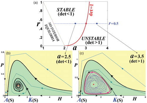
We first focus on the case of one interior equilibrium and show the phase-space portraits when the interior equilibrium is asymptotically stable (i.e. when $det\mathrm{JF}(H_I^{*},P_I^{*})<1$) and unstable (i.e. when $det\mathrm{JF}(H_I^{*},P_I^{*})>1$). In Figure 5, we plot these portraits for (a = 2.5, r = 0.5) and (a = 3.5, r = 0.5) that correspond to a stable and unstable interior equilibrium, respectively.

Figure 5. Phase-space portraits with stable and unstable interior equilibrium. (a) The parameter space (a,r) is plotted (similar to Figure 4(a)) for $H_{\mathrm{ref}}=1/(s\gamma )=1$ ( s = 0.5,γ = 2). On the line r = 0.5, we pick (b) a = 2.5 and (c) a = 3.5 corresponding to $det\mathrm{JF}(H_I^{*},P_I^{*})<1$ and $det\mathrm{JF}(H_I^{*},P_I^{*})>1$, and plot the phase-space portraits that are characterized by a stable and an unstable interior equilibrium, respectively. The unstable interior equilibrium is surrounded by an invariant loop (red closed curve). (Yellow: extinction region; green: coexistence region.)

The unstable manifold of the carrying capacity K is reproduced after 10³ iterations of 10³ initial points equidistributed along the direction of the respective eigenvector and within a length ∼10⁻⁶ starting from K. In the same way, we can numerically find the unstable manifold when (a) $det\mathrm{JF}(H_I^{*},P_I^{*})<1$ and (b) $det\mathrm{JF}(H_I^{*},P_I^{*})>1$. In the first case, the unstable manifold starting from K converges to the stable interior equilibrium I, while in the second case, the unstable manifold starting from I converges to an invariant loop around the unstable interior equilibrium. Then, the same method is used to find the invariant loop (invariant closed curve), with the difference that the initial 90% of the iterations are discarded. The stable invariant curve that connects with the Allee threshold (A,0) cannot be reproduced using the same method, because iterated points converge to A. However, the method can be applied using the inverse map, (39a) $\begin{array}{rl}(H_{t+1},P_{t+1})& =F^{-1}(H_t,P_t)\equiv [f_1^{-1}(H_t,P_t),f_2^{-1}(H_t,P_t)],\end{array}$(39a) (39b) $\begin{array}{rl}\mathrm{with}{f}_1^{-1}(H_t,P_t)& \equiv \frac{r-(a/s)P_t-\sqrt{{[r-(a/s)P_t]}^2-4[H_t+(r/s)P_t](H_t-a)}}{2(H_t-a)},\\ f_2^{-1}(H_t,P_t)& \equiv -\frac{1}{\lambda }\ln \left[H_t\left(1-\frac{P_t}{s{H}_{t+1}}\right)\right].\end{array}$(39b)

Now, under the inverse map, the stable manifold of A under the map F (13) becomes the unstable manifold of A under the map F⁻¹ (39a,b).

The existence of the interior equilibrium allows five different types of phase-space portraits, two for the case of stable interior equilibrium, and three for the case of unstable interior equilibrium. These are always characterized by an extinction region, and they may also have a coexistence region. (For more details on the extinction, exclusion, and coexistence regions, see [29])

• Portraits for a stable interior equilibrium: In the case of a stable interior equilibrium, there are two types of phase-space portraits, corresponding to a stable interior equilibrium with (i) real eigenvalues, when $(det-\frac{1}{4}{\mathrm{Tr}}^2)\mathrm{JF}(H_I^{*},P_I^{*})<0$, as shown in Figure 6(a), or with (ii) complex eigenvalues, when $(det-\frac{1}{4}{\mathrm{Tr}}^2)\mathrm{JF}(H_I^{*},P_I^{*})>0$, as shown in Figure 5(b) and Figures 6(b) and 6(c).

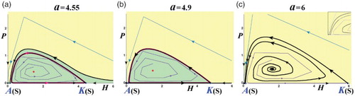
• Portraits for an unstable interior equilibrium: Three other types exist when the interior equilibrium is unstable: (iii) when there is a invariant loop (supercritical Neimark–Sacker bifurcation), as shown in Figures 5(c) and 7(a); (iv) when the invariant loop expands to the whole area between the invariant curves of A and K (Figure 7(b)), and (v) when there is no invariant loop (Figure 7(c)).

Figure 6. Phase-space portraits with a stable interior equilibrium (s = 0.5, γ = 1.8, r = 0.75; $H_{\mathrm{ref}}=1/(s\gamma )=1\frac{1}{9}$). The interior equilibrium can have either real eigenvalues, for example, for (a) a = 1.42, or complex eigenvalues, for example, for (b) a = 1.6 and (c) a = 1.75. (Yellow: extinction region; green: coexistence region.)

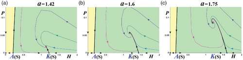
Figure 7. Phase-space portraits with an unstable interior equilibrium (s = 0.5, γ = 2, r = 0.5; $H_{\mathrm{ref}}=1/(s\gamma )=1$). (a) The unstable interior equilibrium is surrounded by an invariant loop similar to Figure 5(c), but for even higher values of $det\mathrm{JF}(H_I^{*},P_I^{*})>1$. (b) The invariant loop expands to the whole area between the invariant curves of A and K. Because of the infinite time that orbits need to reach exactly the invariant loop, the region inside the invariant loop is considered to be coexistence. (c) There is no invariant loop (the magnifying panel focus on the area near the Allee threshold). (Yellow: extinction region; green: coexistence region.)

Figure 5 shows the two major types of the dynamics of the interior equilibrium. Figure 5(a) shows three regions in the parameter space (a,r), the no interior equilibrium region, $a<1/(s\gamma )+(1-r)(s\gamma )$, the stability region of the interior equilibrium bounded by the line $a=2/(s\gamma )$ and the curve $(\frac{1}{2}a{)}^2=(1-r)$, and the unstable region bounded by the a-axis and $(\frac{1}{2}a{)}^2>(1-r)$. Figures 5(b) and 5(c) depict the two types, an asymptotically stable interior equilibrium and an unstable interior equilibrium, respectively. Now let us go into further details of the various types of the phase-space portraits. Figures 6 and 7 depict the evolution of the dynamics of the interior equilibrium from the stable node (with real eigenvalues) (Figure 6(a)), to a stable focus (with complex eigenvalues) (Figure 6(b) and (c), and Figure 5(b)). By further increasing the parameter a (i.e. $det\mathrm{JF}(H_I^{*},P_I^{*})$), the interior equilibrium loses its stability and gives rise to the supercritical Neimark–Sacker bifurcation [41,42], which occurs when the modulus of the complex conjugate eigenvalues of $\mathrm{JF}(H_I^{*},P_I^{*})$ is 1, that is, when $det\mathrm{JF}(H_I^{*},P_I^{*})=1$. Here, an invariant loop appears enclosing the interior equilibrium and is formed as the ‘omega limit sets’ [14,15] of the points on the ‘global’ unstable manifold of the carrying capacity K (Figures 7(a) and 5(c)). Increasing further the parameter a, the invariant loop disappears giving rise to a heteroclinic orbit (a separatrix) joining A and K. The coexistence region (green) goes from unbounded, where it lies below the global stable manifold of A, to a region bounded by the heteroclinic orbit joining A and K and the H-axis (Figure 7(b)). Finally, for even large values of a, the invariant loop breaks up and the region of extinction becomes the whole ${\mathrm{\Re }}_{+}^2$ (except from the orbits with initial values on the H-axis with H≥A, and the global stable manifold of A connecting A with the interior equilibrium). For all the various dynamics of one interior equilibrium, it is always the case that both A and K are saddle points. Numerical simulations show that the above types of dynamics are the only possible scenarios and neither new bifurcation nor chaos occurs.

In Figure 6(a), we depict the phase-space portrait for parameter values (a,r) corresponding to the stable region of the interior equilibrium with real eigenvalues, that is, for $(det-\frac{1}{4}{\mathrm{Tr}}^2)\mathrm{JF}(H_I^{*},P_I^{*})<0$. Then, we increase the value of the parameter a, and so of $det\mathrm{JF}(H_I^{*},P_I^{*})$, until the phase-space portrait corresponds to the stable region with complex eigenvalues, that is, for $(det-\frac{1}{4}{\mathrm{Tr}}^2)\mathrm{JF}(H_I^{*},P_I^{*})>0$, as shown in Figure 6(b) and 6(c).

In Figure 7(a), we depict the phase-space portrait for parameter values (a,r) corresponding to the unstable region of the interior equilibrium leading to an invariant loop. Then, we increase the value of the parameter a, and so of $det\mathrm{JF}(H_I^{*},P_I^{*})$, until the invariant loop covers the whole area between the invariant curves of A and K, as shown in Figure 7(b). For even larger values of the parameter a (or of $det\mathrm{JF}(H_I^{*},P_I^{*})$), the invariant loop is being broken and all the orbits tend to the origin, with the exclusion of the H-axis for H≥A (where the orbits tend to K), and the global stable manifold of A (that starts from I and tends to A), as shown in Figure 7(c).

4.2. Portraits with zero interior equilibria

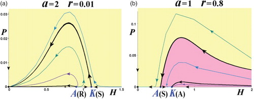
There are another two types of phase-space portraits, that is, when there are no interior equilibria. These are for the conditions (v) H_ref<(A,0)(R)<(K,0)(S), and (vi) (A,0)(S)<(K,0)(A)<H_ref, depicted in Figures 8(a) and 8(b), respectively. The phase-space portrait of the type (v) is all covered by the extinction region, while the type (vi) is the only phase-space portrait with an exclusion region (of the host).

Figure 8. Phase-space portraits with no interior equilibria. (a) Type (v) for H_ref<(A,0)(R)<(K,0)(S), and (b) type (vi) for (A,0)(S)<(K,0)(A)<H_ref. (Yellow: extinction region; red: exclusion region.)

4.3. Summary of the seven types of phase-space portraits

Table 1 assembles all seven types of phase-space portraits discussed in this section. This is by no means inclusive to all possible scenarios.

Table 1. Types of phase-space portraits.

Type	Stability	Conditions	Regions	Description
(i)	(A,0)(S), (K,0)(S), I(A)	A<Href<K, ${\left.(det-\frac{1}{4}{\mathrm{Tr}}^2)\right|}_I<0$, $det{|}_I<1$	Ext; CoE	Stable interior equilibrium is an attractor with real eigenvalues for all the orbits below the interior invariant curve through A (Figure 6(a))
(ii)	(A,0)(S), (K,0)(S), I(A)	A<Href<K, ${\left.(det-\frac{1}{4}{\mathrm{Tr}}^2)\right|}_I>0$, $det{|}_I<1$	Ext; CoE	Stable interior equilibrium is an attractor with complex eigenvalues for all the orbits below the interior invariant curve through A (Figure 6(b))
(iii)	(A,0)(S), (K,0)(S), I(R)	A<Href<K, $det{|}_I>1$	Ext; CoE	Invariant loop (supercritical Neimark–Sacker bifurcation) below the interior invariant curve through A (Figure 7(a))
(iv)	(A,0)(S), (K,0)(S), I(R)	A<Href<K, $det{|}_I>1$	Ext; CoE	Common interior invariant curve through A and K, coinciding with the invariant loop (Figure 7(b))
(v)	(A,0)(S), (K,0)(S), I(R)	A<Href<K, $det{|}_I>1$	Ext	No invariant loop; all orbits lead to origin; the whole phase space is an extinction region (Figure 7(c))
(vi)	(A,0)(R), (K,0)(S)	Href<A	Ext	The interior invariant curves through A and K connects with the origin; the whole phase space is an extinction region (Figure 8(a))
(vii)	(A,0)(R), (K,0)(S)	K<Href	Ext; Exc	K is attractor for all the orbits underneath the interior invariant curve throuth A creating an exclusion region for the host (Figure 8(b))

Note that (1) ${\left.(det-\frac{1}{4}\mathrm{T}{\mathrm{r}}^2)\right|}_I$ and $det{|}_I$ are abbreviations of $(det-\frac{1}{4}\mathrm{T}{\mathrm{r}}^2)\mathrm{JF}(H_I^{*},P_I^{*})$ and $det\mathrm{JF}(H_I^{*},P_I^{*})$, respectively. (2) Ext, CoE, and Exc are abbreviations of extinction, coexistence, and exclusion regions, respectively.

It is worthwhile to explain the differences and similarities among the types (iii), (iv), and (v). In scenario (iii), we observe the formation of the invariant loop caused by the Neimark–Sacker bifurcation. As we increase the value of the parameter a, the invariant loop connects (A,0) and (K,0) resulting in scenario (iv). Increasing further the parameter leads to a global bifurcation of an invariant loop with a saddle chain and the extinction region extends to the whole positive quadrant.

5. Conclusions

In this paper, we proposed a new host–parasitoid model with the Allee effect. The local dynamics of the model have been established in Sections 2 and 3. The global dynamics in Section 4 is based on intensive numerical simulations. Based on our numerical simulations, two scenarios have emerged.

In the first scenario, we have no interior fixed points and there are two associated dynamics. If the second eigenvalues ${\lambda }_2{|}_A$ and ${\lambda }_2{|}_K$ are greater than 1, then the Allee threshold point A is a repeller and the carrying capacity of K is a saddle. This results in the extinction of both host and parasitoid. This case occurs if $s\gamma A=\frac{1}{2}s\gamma [a-\sqrt{a^2-4(1-r)}]>1$. In the second type of dynamics, ${\lambda }_2{|}_A$ and ${\lambda }_2{|}_K$ are less than 1, and A is a saddle and K an attractor. In this case, the non-negative quadrant ${\mathrm{\Re }}_{+}^2$ is divided into two regions: an extinction region (yellow) in the phase-space diagram located above the ‘global’ stable manifold of A, and an exclusion region (red) in which the parasitoid goes to extinction and the host population density (size) approached K. This case occurs if $s\gamma K=\frac{1}{2}s\gamma [a+\sqrt{a^2-4(1-r)}]<1$. This is the only case in which the parasite goes to extinction while the host survives and its population size tends to its carrying capacity K. This phenomenon is caused by a combination of low Allee effect intensity and high growth rate of the host.

In the second scenario, we have one interior fixed point. This occurs only if ${\lambda }_2{|}_A<1$ and ${\lambda }_2{|}_K>1$, that is, if both A and K are saddle points. Explicitly, we then have $s\gamma A=\frac{1}{2}s\gamma [a-\sqrt{a^2-4(1-r)}]<1$ and $s\gamma K=\frac{1}{2}s\gamma [a+\sqrt{a^2-4(1-r)}]>1$. The interior fixed point is locally asymptotically stable and the coexistence region in the phase-space diagram (Figures 5(b) and 6) is bounded by the global stable manifold of the Allee threshold point A and the H-axis. By increasing the parameter a, and thus increasing the intensity of the Allee effect, the interior fixed point loses its stability which gives rise to an attracting invariant loop. The extinction region in the above two cases lies above the global stable manifold of the Allee threshold point A. Notice that the appearance of the invariant loop is caused by the Neimark–Sacker bifurcation, which occurs when the modulus of the complex eigenvalues of the Jacobian crosses unity [13,18,41,42]. By increasing the parameter a, numerical simulations show a global bifurcation of an invariant loop with a saddle chain (Figure 7(a) and 7(b)), where both species go extinct (Figure 7(c)). The latter case is due to the presence of a severe Allee effect on the host (e.g. a∼2⁺, r∼0). Mathematical analysis and investigation of these fascinating dynamics have yet to be established.

We conclude, from our study, that the combined effect of parasitism and the Allee effect is not only deleterious for the host, but it also has a devastating effect on the parasite. So it may be seen from Figures 5 and 7 that the extinction region of both species is unbounded, which leads us to conclude that the probability that both the host and the parasitoid (or just the host) survive is rather small, tending asymptotically to zero with the increase of the intensity of the Allee effect.

Acknowledgement

This research was supported by a grant from King Abdul-Aziz University.

Appendix.

The appendix provides Lemmas A1–A4 with their proofs.

Lemma

Let S₁ and S₂ be the slopes of the two isoclines C₁ and C₂ at A or K, that is, $S_1=P_1^{\mathrm{\prime }}(H^{*})$, $S_2=P_2^{\mathrm{\prime }}(H^{*})$, with $H^{*}=A,K$. Then, their ratio is given by (A1) $\frac{S_1}{S_2}=\frac{1}{s\gamma H^{*}},\mathrm{that}\mathrm{is},{\left.\frac{S_1}{S_2}\right|}_A=\frac{1}{\gamma sA},{\left.\frac{S_1}{S_2}\right|}_K=\frac{1}{s\gamma K}.$(A1)

Proof

The proof is straightforward and omitted.

Lemma

We define the quantity (A2) $\sigma \equiv \left({\left.\frac{S_1}{S_2}\right|}_A-1\right)\cdot \left({\left.\frac{S_1}{S_2}\right|}_K-1\right).$(A2)

If σ>0, then there is either zero or two interior equilibria; if σ<0, then there is one interior equilibrium. Note that if $(S_1/S_2){|}_A=1$ and/or $(S_1/S_2){|}_K=1$, then the ratio of slopes that is equal to zero must be replaced by the ratio of higher order derivatives (non-zero derivatives of smallest order).

Proof

The slopes of the two isoclines at $H^{*}=A,K$, S₁, and S₂, have the same signs. Thus, their ratio is positive, $(S_1/S_2){|}_{A,K}>0$. More precisely, the slopes are positive at A and negative at K. Thus, if S₁ > S₂ for both A and K, there can be either zero or two points of intersections of C₁ and C₂. If S₁ > S₂ for A and S₁ < S₂ for K (or vice versa), then there is one point of intersection of C₁ and C₂ (there cannot be three points of intersections because the curves have one maximum value for A<H<K). For example, if $s\gamma A<1$ and $s\gamma K>1$, then, according to Lemma A1, we have $(S_1/S_2){|}_A>1$ and $(S_1/S_2){|}_K<1$, thus, there is one interior equilibrium.

Lemma

If $s\gamma A>1$, then there are no interior equilibria.

Proof

From Lemma A2 we have that, if $s\gamma A>1$, then $(S_1/S_2){|}_A<1$. Also, $s\gamma K>s\gamma A>1$, then $(S_1/S_2){|}_K<1$. Hence, there is either zero or two interior equilibria. However, below we show that, if $s\gamma A>1$, then no interior equilibria can exist.

The function $u(H)$ becomes zero at $H=A,K$ and has a maximum at $H=H_{\mathrm{c}}$, where (A3) $\begin{array}{rl}u(H)& \equiv \frac{aH+r}{1+H^2},\end{array}$(A3) (A4) $\begin{array}{rl}{H}_{\mathrm{c}}& \equiv -\frac{r}{a}+\sqrt{{\left(\frac{r}{a}\right)}^2+1},u_{\mathrm{c}}\equiv u(H_{\mathrm{c}})=\frac{a}{2H_{\mathrm{c}}}.\end{array}$(A4)

Note that H_c is also the maximum of the isocline C₁.

The function $u(H)$ is the fitness of the host in the absence of the parasite [15]. It is monotonically increasing and concave in the interval $A<H\le H_{\mathrm{c}}$. Hence, $u(A)=1\le u(H)$ and $u^{\mathrm{\prime }}(A)\ge u^{\mathrm{\prime }}(H)$ or $H^{\mathrm{\prime }}(u)\ge 1/u^{\mathrm{\prime }}(A)$. Let the function G(H) be defined by (A5) $G(H)\equiv \frac{1}{H}\cdot \frac{\ln u(H)}{1-1/u(H)}.$(A5)

Then, we have (A6) $\begin{array}{r}\begin{array}{rl}\frac{\mathrm{d}}{\mathrm{d}H}G(H)& =u^{\mathrm{\prime }}(H)\cdot \frac{\mathrm{d}}{\mathrm{d}u}G[H(u)]=\frac{1}{H(u)(u-1)H^{\mathrm{\prime }}(u)}\cdot \left[-\frac{u\ln u{H}^{\mathrm{\prime }}(u)}{H(u)}+\frac{u-1-\ln u}{u-1}\right]\\ & =\frac{1}{H(u)(u-1)H^{\mathrm{\prime }}(u)}\cdot \left[-\frac{u\ln u{H}^{\mathrm{\prime }}(u)}{H(u)}+1-\frac{1}{u}\cdot \frac{\ln u}{1-1/u}\right].\end{array}\end{array}$(A6)

Then, because of $-H^{\mathrm{\prime }}(u)\le -1/u^{\mathrm{\prime }}(A)<0$, and $\ln u\cdot (1-1/u{)}^{-1}\ge 1$ or $1-\ln u\cdot (1-1/u{)}^{-1}\le 0$, (A7) $G^{\mathrm{\prime }}(H)<0,A\le H\le H_{\mathrm{c}}.$(A7)

Also, $u(H)$ is monotonically decreasing and concave in the interval $H_{\mathrm{c}}<H\le K$, that is, $H^{\mathrm{\prime }}(u)<0$, (A8) $\frac{\mathrm{d}}{\mathrm{d}H}G(H)=\frac{1}{H(u)(u-1)}\cdot \left[-\frac{u\ln u}{H(u)}-\left(1-\frac{\ln u}{u-1}\right)\cdot \frac{1}{|H^{\mathrm{\prime }}(u)|}\right]<0,$(A8) because $\ln u/(u-1)<1$; hence, (A9) $G^{\mathrm{\prime }}(H)<0,H_{\mathrm{c}}\le H\le K.$(A9)

Therefore, G(H) is monotonically decreasing function for any H in the interval $A\le H\le H_{\mathrm{c}}$. Hence, $G(A)\ge G(H)$, for any $A\le H\le K$, which is rewritten as (A10) $\frac{1}{A}\ge \frac{1}{H}\cdot \frac{\ln u(H)}{1-1/u(H)},$(A10) where we used $\ln u(A)/[1-1/u(A)]=1$. Therefore, there is no value x, so that (A11) $\frac{1}{A}<x<\frac{1}{H}\cdot \frac{\ln u(H)}{1-1/u(H)},\mathrm{for}\mathrm{any}H:A<H\le K.$(A11)

Then, we set $x=s\cdot \gamma$ and we obtain that, there is no value of the parameter product $s\gamma$ so that $1<s\gamma A$ and $s\gamma H<\ln u(H)/[1-1/u(H)]$ with $A<H\le K$. Evidently, if $1<s\gamma A$, then we must have (A12) $s\gamma H>\frac{\ln u(H)}{1-1/u(H)},\mathrm{or}\frac{1}{s\gamma H}\cdot \frac{\ln u(H)}{1-1/u(H)}>1,\mathrm{for}\mathrm{any}A\le H\le K.$(A12)

Given that (A13) $\frac{P_1(H)}{P_2(H)}=\frac{1}{s\gamma H}\cdot \frac{\ln u(H)}{1-1/u(H)},$(A13) we obtain (A14) $P_1(H)>P_2(H),\mathrm{for}\mathrm{any}A\le H\le K.$(A14)

Namely, the two isoclines do not intersect for any H: $A\le H\le K$. Thus, there are no interior equilibria.

Lemma

If $s\gamma K<1$, then there are no interior equilibria.

Proof

From Lemma A2 we have that, if $s\gamma K<1$, then $(S_1/S_2){|}_K>1$. Also, $s\gamma A<s\gamma K<1$, thus $(S_1/S_2){|}_A>1$. Hence, there can be either zero or two interior equilibria. Furthermore, given Equation (A12), we have (A15) $\frac{P_1(H)}{P_2(H)}=\frac{1}{s\gamma H}\cdot \frac{\ln u(H)}{1-1/u(H)}>\frac{1}{s\gamma H}>\frac{1}{s\gamma K}>1,$(A15) and, consequently, there are no interior equilibria.

References

- W.C. Allee, Animal Aggregations, a Study in General Sociology, University of Chicago Press, Chicago, IL, 1931.
- L.J.S. Allen, J.F. Fagan, G. Högnäsc, and H. Fagerholmc, Population extinction in discrete-time stochastic population models with an Allee effect, J. Difference Equ. Appl. 11 (2005), pp. 273–293. doi: 10.1080/10236190412331335373
- R. Asheghi, Bifurcation and dynamics of a discrete predator-prey system, J. Biol. Dyn. 8 (2014), pp. 161–186. doi: 10.1080/17513758.2014.927596
- L. Assas, S. Elaydi, G. Livadiotis, E. Kwessi, and D. Ribble, Hierarchical competition models with Allee effects, J. Biol. Dyn. (2014). doi:10.1080/17513758.2014.923118
- J.R. Beddington, C.A. Free, and J.H. Lawton, Dynamic complexity in predator-prey models framed in difference equations, Nature 225 (1975), pp. 58–60. doi: 10.1038/255058a0
- T. Bellows, The descriptive properties of some models for density dependence, J. Anim. Ecol. 50 (1981), pp. 139–156. doi: 10.2307/4037
- A. Bompard, I. Amat, X. Fauvergue, and T. Spataro, Host-parasitoid dynamics and the success of biological control when parasitoids are prone to Allee effects, PLoS ONE 8 (2013), p. e76768. doi: 10.1371/journal.pone.0076768
- D.S. Boukal, M.W. Sabelis, and L. Berec, How predator functional responses and Allee effects in prey affect the paradox of enrichment and population collapses, Theor. Popul. Biol. 72 (2007), pp. 136–147. doi: 10.1016/j.tpb.2006.12.003
- F. Courchamp, L. Berec, and J. Gascoigne, Allee Effects in Ecology and Conservations, Oxford University Press, Oxford, 2008.
- B. Dennis, Allee effects: Population growth, critical density, and the chance of extinction, Nat. Resour. Model. 3 (1989), pp. 481–538.
- B. Dennis, Allee effects in stochastic populations, Oikos 96 (2002), pp. 389–401. doi: 10.1034/j.1600-0706.2002.960301.x
- A. Deredec and F. Courchamp, Combined impacts of Allee effects and parasitism, Oikos 112 (2006), pp. 667–679. doi: 10.1111/j.0030-1299.2006.14243.x
- S. Elaydi, An Introduction to Difference Equations, 3rd ed., Springer-Verlag, New York, 2005.
- S. Elaydi, Discrete Chaos: With Applications in Science and Engineering, 2nd ed., Chapman & Hall/CRC, Boca Raton, FL, 2008.
- S. Elaydi and R.J. Sacker, Population models with Allee effect: A new model, J. Biol. Dyn. 4 (2010), pp. 397–408. doi: 10.1080/17513750903377434
- J. Gascoigne and R. Lipccius, Allee effect driven by predation, J. Appl. Ecol. 41 (2004), pp. 801–810. doi: 10.1111/j.0021-8901.2004.00944.x
- M. Groom, Alee effects limit population viability of an annual plant, Amer. Nat. 151 (1998), pp. 487–496. doi: 10.1086/286135
- A.N.W. Hone, M.V. Irle, and G.W. Thurura, On the Neimark-Sacker bifurcation in a discrete predator-prey system, J. Biol. Dyn. 4 (2010), pp. 594–606. doi: 10.1080/17513750903528192
- S. Jang, Discrete-time host-parasitoid models with Allee effects: Density dependence versus parasitism, J. Difference Equ. Appl. 17 (2011), pp. 525–539. doi: 10.1080/10236190903146920
- S. Jang, Allee effects in a discrete-time host-parasitoid model, J. Difference Equ. Appl. 12 (2006), pp. 165–181. doi: 10.1080/10236190500539238
- S. Jang and S. Diamond, A host-parasitoid interaction with Allee effects on the host, Comput. Math. Appl. 53 (2007), pp. 89–103. doi: 10.1016/j.camwa.2006.12.013
- Y. Kang and A.A. Yakubu, Weak Allee effects and species coexistence, Nonlinear Anal. Real World App. 12 (2011), pp. 3329–3345, (2008), pp. 89–101.
- Y. Kang, D. Armbruster, and Y. Kuang, Dynamics of plant herbivore model, J. Biol. Dyn. 2 (2008), pp. 89–101. doi: 10.1080/17513750801956313
- S. Kapcak, V. Ufuktube, and S. Elaydi, Stability and invariant manifolds of a generalized Beddington host-parasitoid model, J. Biol. Dyn. 7 (2013), pp. 233–253. doi: 10.1080/17513758.2013.849764
- A. Kent, C. Doncaster, and T. Sluckin, Consequences for predators of rescue and Allee effects on prey, Ecol. Mod. 162 (2003), pp. 233–245. doi: 10.1016/S0304-3800(02)00343-5
- J. Li, B. Song, and X. Want, An extended discrete Ricker population model with Allee effects, J. Difference Equ. Appl. 13 (2007), pp. 309–321. doi: 10.1080/10236190601079191
- J. Liu, Z. Li, M. Gao, H. Dai, and Z. Liu, Dynamics of a host-parasitoid model with Allee effect for the host and parasitoid aggregation, Ecol. Complex. 6 (2009), pp. 337–345. doi: 10.1016/j.ecocom.2009.01.003
- G. Livadiotis, Approach on Tsallis statistical interpretation of hydrogen-atom by adopting the generalized radial distribution function, J. Math. Chem. 45 (2009), pp. 930–939. doi: 10.1007/s10910-009-9524-6
- G. Livadiotis and S. Elaydi, General Allee effect in two-species population biology, J. Biol. Dyn. 6 (2012), pp. 959–973. doi: 10.1080/17513758.2012.700075
- G. Livadiotis and D.J. McComas, Beyond kappa distributions: Exploiting Tsallis statistical mechanics in space plasmas, J. Geophys. Res. 114 (2009), p. A11105. doi: 10.1029/2009JA014352
- G. Livadiotis and D.J. McComas, Measure of the departure of the q-metastable stationary states from equilibrium, Phys. Scr. 82 (2010), p. 035003. doi: 10.1088/0031-8949/82/03/035003
- G. Livadiotis and D.J. McComas, Non-equilibrium thermodynamic processes: Space plasmas and the inner heliosheath, Astrophys. J. 749 (2012), p. 11 51. doi: 10.1088/0004-637X/749/1/11
- G. Livadiotis, L. Assas, S. Elaydi, E. Kwessi, and D. Ribble, Competition models with Alee effects, J. Difference Equ. Appl. 20 (2014), pp. 1127–1151. doi: 10.1080/10236198.2014.897341
- R.M. May, Host-parasitoid systems in patchy environments: A phenomenological model, J. Anim. Ecol. 47 (1978), pp. 833–844. doi: 10.2307/3674
- R. May, M.P. Hassell, R.M. Anderson, and D.W. Tonkyn, Density dependence in host-parasitoid models, J. Anim. Ecol. 50 (1981), pp. 855–865. doi: 10.2307/4142
- M.A. McCarthy, The Allee effect, finding maths and theoretical models, Ecol. Model. 103 (1997), pp. 99–102. doi: 10.1016/S0304-3800(97)00104-X
- A. Morozov, S. Petrovskii, and B.L. Li, Bifurcations, and chaos in a predator-prey system with the Allee effect, Proc. R. Soc. B. 271 (2004), pp. 1407–1414. doi: 10.1098/rspb.2004.2733
- A. Nicholson and V. Bailey, The balance of animal populations, Proc. Zool. Soc. London 105(3) (1935), pp. 551–598. doi: 10.1111/j.1096-3642.1935.tb01680.x
- L. Rodrigues, D. Mistro, and S. Petroviskii, Pattern formation in a space and time-discrete predator-prey system with a strong Allee effect, Theor. Ecol. 5 (2012), pp. 341–362. doi: 10.1007/s12080-011-0139-8
- G. Roth, and S. Schreiber, Pushed beyond the brink: Allee effects, environmental stochasticity, and extinction, J. Biol. Dyn. (2014). doi:10.1101/004887
- R.J. Sacker, Introduction to the 2009 re-publication of the ‘Neimark-Sacker bifurcation theorem’, J. Difference Equ. Appl. 15 (2009), pp. 753–758. doi: 10.1080/10236190802357750
- R.J. Sacker, On invariant surfaces and bifurcation of periodic solutions of ordinary differential equations, J. Difference Equ. Appl. 15 (2009), pp. 759–774. doi: 10.1080/10236190802357735
- S.J. Schreiber, Allee effects, extinctions, and chaotic transients in simple population models, Theor. Popul. Biol. 64 (2003), pp. 201–209. doi: 10.1016/S0040-5809(03)00072-8
- P.A. Stephens and W.J. Sutherland, Consequences of the Allee effect for behavior, ecology and conservation, Trends Ecol. Evol. 14 (1999), pp. 401–405. doi: 10.1016/S0169-5347(99)01684-5
- H.R. Thieme, T. Dhirasakdanon, Z. Han, and R. Trevino, Species decline and extinction: Synergy of infectious diseases and Allee effect, J. Biol. Dyn. 3 (2009), pp. 305–323. doi: 10.1080/17513750802376313
- C. Tsallis, Possible generalization of Boltzmann-Gibbs statistics, J. Stat. Phys. 52 (1988), pp. 479–487. doi: 10.1007/BF01016429
- G.A. van Voorn, L. Hemerik, M. Boer, and B. Kooi, Heteroclinic orbits indicate overexploitation in predator-prey systems with a strong Allee effect, Math. Biosci. 209 (2007), pp. 451–469. doi: 10.1016/j.mbs.2007.02.006
- S. Zhou, Y. Liu, and G. Wang, The stability of predator-prey systems subject to the Allee effects, Theor. Popul. Biol. 67 (2005), pp. 23–31. doi: 10.1016/j.tpb.2004.06.007