Global behaviour of a predator–prey like model with piecewise constant arguments

Abstract

The present study deals with the analysis of a predator–prey like model consisting of system of differential equations with piecewise constant arguments. A solution of the system with piecewise constant arguments leads to a system of difference equations which is examined to study boundedness, local and global asymptotic behaviour of the positive solutions. Using Schur–Cohn criterion and a Lyapunov function, we derive sufficient conditions under which the positive equilibrium point is local and global asymptotically stable. Moreover, we show numerically that periodic solutions arise as a consequence of Neimark-Sacker bifurcation of a limit cycle.

Keywords:

• piecewise constant arguments
• difference equation
• stability
• bifurcation

AMS Subject Classification:

• 39A10
• 39A28
• 39A30

1. Introduction

Recently, there has been great interest in studying differential equations with piecewise constant arguments because of the wide application of these equations in biology, engineering and other fields. Many authors have analysed various types of population models based on logistic equations with piecewise constant arguments and have obtained theoretical results on oscillations or chaotic behaviour [2,4–6,8–14,15,16]. The simplest model was proposed by May [9] and May and Oster [10] who obtained that the model have chaotic behaviour for certain parameters. On the other hand, several authors [8,11,12,15,16] have investigated a more general logistic equation with piecewise constant arguments (1) $\frac{\mathrm{d}x\left(t\right)}{\mathrm{d}t}=rx\left(t\right)(1-ax(t)-b\sum _{j=0}^m{c}_{j}x([t-j]\left)\right),t\ge 0.$(1) Liu and Gopalsamy [8] have showed that for certain special cases, solutions of equation (1(1) $\frac{\mathrm{d}x\left(t\right)}{\mathrm{d}t}=rx\left(t\right)(1-ax(t)-b\sum _{j=0}^m{c}_{j}x([t-j]\left)\right),t\ge 0.$(1) ) can have chaotic behaviour through period doubling bifurcations. Muroya [12] has improved contractivity conditions for the positive equilibrium point of this equation.

Following these works, Gurcan and Bozkurt [5] have studied global stability and boundedness character of the positive solutions of the differential equation (2) $\frac{\mathrm{d}x\left(t\right)}{\mathrm{d}t}=rx\left(t\right)(1-\alpha x(t)-{\beta }_{0}x(\left[t\right])-{\beta }_{1}x([t-1]\left)\right).$(2) By using this equation, Ozturk et al. [14] have modelled a population density of a bacteria species in a microcosm. A more general case of equation (2(2) $\frac{\mathrm{d}x\left(t\right)}{\mathrm{d}t}=rx\left(t\right)(1-\alpha x(t)-{\beta }_{0}x(\left[t\right])-{\beta }_{1}x([t-1]\left)\right).$(2) ) has been considered by Ozturk and Bozkurt [13] as the following; (3) $\frac{\mathrm{d}x\left(t\right)}{\mathrm{d}t}=x\left(t\right)\left(r\right(1-\alpha x\left(t\right)-{\beta }_{0}x\left(\right[t\left]\right)-{\beta }_{1}x\left(\right[t-1\left]\right))+{\gamma }_{1}x(\left[t\right])+{\gamma }_{2}x([t-1]\left)\right).$(3) They have investigated stability and oscillatory characteristics of difference solutions of the equation. Equation (3(3) $\frac{\mathrm{d}x\left(t\right)}{\mathrm{d}t}=x\left(t\right)\left(r\right(1-\alpha x\left(t\right)-{\beta }_{0}x\left(\right[t\left]\right)-{\beta }_{1}x\left(\right[t-1\left]\right))+{\gamma }_{1}x(\left[t\right])+{\gamma }_{2}x([t-1]\left)\right).$(3) ) has also been used for modelling an early brain tumour growth in [2]. The stability analysis of the model shows that increase in the tumour growth rate decreases the local stability of the positive equilibrium point. Another mathematical model for tumour growth under the immune activity has been constructed Banerjee and Sarkar [1] such as (4) $\begin{array}{rl}\frac{\mathrm{d}M}{\mathrm{d}t}& =r_{1}M\left(1-\frac{M}{k_1}\right)-{\alpha }_{1}MN,\\ \frac{\mathrm{d}N}{\mathrm{d}t}& =\beta NZ(t-\tau )-d_{1}N-{\alpha }_{2}MN,\\ \frac{\mathrm{d}Z}{\mathrm{d}t}& =r_{2}Z\left(1-\frac{Z}{k_2}\right)-\beta NZ(t-\tau ),\end{array}$(4) where $M\left(t\right)$, $N\left(t\right)$, $Z\left(t\right)$ represent the number of tumour, hunting and resting cells, respectively. The model consists of delay differential equations which often arise in biological systems. Since analysis of these equations is more complicated than ordinary differential equations, numerical approach may be needed for delay differential equations. In study [3], Cooke and Györi have showed that differential equations with piecewise constant arguments can be used to obtain approximate solution to delay differential equations that contain discrete delays.

In the present paper, we have modified model (4(4) $\begin{array}{rl}\frac{\mathrm{d}M}{\mathrm{d}t}& =r_{1}M\left(1-\frac{M}{k_1}\right)-{\alpha }_{1}MN,\\ \frac{\mathrm{d}N}{\mathrm{d}t}& =\beta NZ(t-\tau )-d_{1}N-{\alpha }_{2}MN,\\ \frac{\mathrm{d}Z}{\mathrm{d}t}& =r_{2}Z\left(1-\frac{Z}{k_2}\right)-\beta NZ(t-\tau ),\end{array}$(4) ) by adding piecewise constant arguments such as (5) $\begin{array}{rl}\frac{\mathrm{d}M}{\mathrm{d}t}& =r_{1}M\left(t\right)\left(1-\frac{M\left(t\right)}{k_1}\right)-{\alpha }_{1}M\left(t\right)N\left(\right[t\left]\right),\\ \frac{\mathrm{d}N}{\mathrm{d}t}& =\beta N\left(t\right)Z\left(\right[t\left]\right)-d_{1}N\left(t\right)-{\alpha }_{2}M\left(\right[t\left]\right)N\left(t\right),\\ \frac{\mathrm{d}Z}{\mathrm{d}t}& =r_{2}Z\left(t\right)\left(1-\frac{Z\left(t\right)}{k_2}\right)-\beta N\left(\right[t\left]\right)Z\left(t\right),\end{array}$(5) where $\left[t\right]$ denotes the integer part of $t\in [0,\mathrm{\infty })$ and all these parameters are positive. The model includes both discrete and continuous time for tumour, hunting and resting cells because tumour cells have different dynamics which can be described by using both differential and difference equations. Here, $M\left(t\right)$, $N\left(t\right)$ and $Z\left(t\right)$ represent population density of tumour, hunting and resting cells, respectively. The parameters $r_1$ and $k_1$ represent the growth rate and the maximum carrying capacity of tumour cells, respectively. $r_2$ is the growth rate, $k_2$ is the maximum carrying capacity of resting cells and $d_1$ is the natural death of hunting cell. The parameter ${\alpha }_1$ denotes decay rate of tumour cells by hunting cells, ${\alpha }_2$ is decay rate of hunting cells by tumour cells and β is conversion rate from resting to hunting cells. Most of the parameter values are taken from the [1] in terms of consistency with the biological facts. In Section 2, we investigate boundedness, local and global behaviour of the positive solutions of the system by using the method of reduction to discrete equations. In Section 3, we study periodic solution of the system through Neimark-Sacker bifurcation.

2. Boundedness, local and global stability analysis

In this section, by integrating of system (5(5) $\begin{array}{rl}\frac{\mathrm{d}M}{\mathrm{d}t}& =r_{1}M\left(t\right)\left(1-\frac{M\left(t\right)}{k_1}\right)-{\alpha }_{1}M\left(t\right)N\left(\right[t\left]\right),\\ \frac{\mathrm{d}N}{\mathrm{d}t}& =\beta N\left(t\right)Z\left(\right[t\left]\right)-d_{1}N\left(t\right)-{\alpha }_{2}M\left(\right[t\left]\right)N\left(t\right),\\ \frac{\mathrm{d}Z}{\mathrm{d}t}& =r_{2}Z\left(t\right)\left(1-\frac{Z\left(t\right)}{k_2}\right)-\beta N\left(\right[t\left]\right)Z\left(t\right),\end{array}$(5) ) we first obtain a solution and later discuss the boundedness and the local asymptotic stability of system (7(7) $\begin{array}{rl}M(n+1)& =\frac{M\left(n\right)(r_1-{\alpha }_{1}N(n\left)\right)}{r_1{K}_{1}M\left(n\right)+(r_1-{\alpha }_{1}N(n)-r_1{K}_{1}M(n\left)\right)\exp (-(r_1-{\alpha }_{1}N\left(n\right)\left)\right)},\\ N(n+1)& =N\left(n\right)\exp \left(\beta Z\right(n)-d_1-{\alpha }_{2}M(n\left)\right),\\ Z(n+1)& =\frac{Z\left(n\right)(r_2-\beta N(n\left)\right)}{r_2{K}_{2}Z\left(n\right)+(r_2-\beta N(n)-r_2{K}_{2}Z(n\left)\right)\exp (-(r_2-\beta N\left(n\right)\left)\right)},\end{array}$(7) ).

We can rewrite system (5(5) $\begin{array}{rl}\frac{\mathrm{d}M}{\mathrm{d}t}& =r_{1}M\left(t\right)\left(1-\frac{M\left(t\right)}{k_1}\right)-{\alpha }_{1}M\left(t\right)N\left(\right[t\left]\right),\\ \frac{\mathrm{d}N}{\mathrm{d}t}& =\beta N\left(t\right)Z\left(\right[t\left]\right)-d_{1}N\left(t\right)-{\alpha }_{2}M\left(\right[t\left]\right)N\left(t\right),\\ \frac{\mathrm{d}Z}{\mathrm{d}t}& =r_{2}Z\left(t\right)\left(1-\frac{Z\left(t\right)}{k_2}\right)-\beta N\left(\right[t\left]\right)Z\left(t\right),\end{array}$(5) ) on an interval of the form $t\in [n,n+1)$ as follows: (6) $\begin{array}{rl}\frac{\mathrm{d}M}{\mathrm{d}t}& =r_{1}M\left(t\right)\left(1-\frac{M\left(t\right)}{k_1}\right)-{\alpha }_{1}M\left(t\right)N\left(n\right),\\ \frac{\mathrm{d}N}{\mathrm{d}t}& =\beta N\left(t\right)Z\left(n\right)-d_{1}N\left(t\right)-{\alpha }_{2}M\left(n\right)N\left(t\right),\\ \frac{\mathrm{d}Z}{\mathrm{d}t}& =r_{2}Z\left(t\right)\left(1-\frac{Z\left(t\right)}{k_2}\right)-\beta N\left(n\right)Z\left(t\right).\end{array}$(6) By solving each equations in the system (6(6) $\begin{array}{rl}\frac{\mathrm{d}M}{\mathrm{d}t}& =r_{1}M\left(t\right)\left(1-\frac{M\left(t\right)}{k_1}\right)-{\alpha }_{1}M\left(t\right)N\left(n\right),\\ \frac{\mathrm{d}N}{\mathrm{d}t}& =\beta N\left(t\right)Z\left(n\right)-d_{1}N\left(t\right)-{\alpha }_{2}M\left(n\right)N\left(t\right),\\ \frac{\mathrm{d}Z}{\mathrm{d}t}& =r_{2}Z\left(t\right)\left(1-\frac{Z\left(t\right)}{k_2}\right)-\beta N\left(n\right)Z\left(t\right).\end{array}$(6) ) with respect to t on $[n,t)$ and letting $t\to n+1$, we obtain a system of difference equations (7) $\begin{array}{rl}M(n+1)& =\frac{M\left(n\right)(r_1-{\alpha }_{1}N(n\left)\right)}{r_1{K}_{1}M\left(n\right)+(r_1-{\alpha }_{1}N(n)-r_1{K}_{1}M(n\left)\right)\exp (-(r_1-{\alpha }_{1}N\left(n\right)\left)\right)},\\ N(n+1)& =N\left(n\right)\exp \left(\beta Z\right(n)-d_1-{\alpha }_{2}M(n\left)\right),\\ Z(n+1)& =\frac{Z\left(n\right)(r_2-\beta N(n\left)\right)}{r_2{K}_{2}Z\left(n\right)+(r_2-\beta N(n)-r_2{K}_{2}Z(n\left)\right)\exp (-(r_2-\beta N\left(n\right)\left)\right)},\end{array}$(7) where $1/k_1=K_1$, $1/k_2=K_2$. Thus, we obtain discrete analogue of system (5(5) $\begin{array}{rl}\frac{\mathrm{d}M}{\mathrm{d}t}& =r_{1}M\left(t\right)\left(1-\frac{M\left(t\right)}{k_1}\right)-{\alpha }_{1}M\left(t\right)N\left(\right[t\left]\right),\\ \frac{\mathrm{d}N}{\mathrm{d}t}& =\beta N\left(t\right)Z\left(\right[t\left]\right)-d_{1}N\left(t\right)-{\alpha }_{2}M\left(\right[t\left]\right)N\left(t\right),\\ \frac{\mathrm{d}Z}{\mathrm{d}t}& =r_{2}Z\left(t\right)\left(1-\frac{Z\left(t\right)}{k_2}\right)-\beta N\left(\right[t\left]\right)Z\left(t\right),\end{array}$(5) ) as a system of difference equation which reveals the rich dynamical characteristics and the asymptotic behaviour of the dynamical system (5(5) $\begin{array}{rl}\frac{\mathrm{d}M}{\mathrm{d}t}& =r_{1}M\left(t\right)\left(1-\frac{M\left(t\right)}{k_1}\right)-{\alpha }_{1}M\left(t\right)N\left(\right[t\left]\right),\\ \frac{\mathrm{d}N}{\mathrm{d}t}& =\beta N\left(t\right)Z\left(\right[t\left]\right)-d_{1}N\left(t\right)-{\alpha }_{2}M\left(\right[t\left]\right)N\left(t\right),\\ \frac{\mathrm{d}Z}{\mathrm{d}t}& =r_{2}Z\left(t\right)\left(1-\frac{Z\left(t\right)}{k_2}\right)-\beta N\left(\right[t\left]\right)Z\left(t\right),\end{array}$(5) ). Now, we can discuss the boundedness of solutions of the system in the following theorem.

Theorem 2.1.

Let $\left\{M\right(n),N(n),Z(n){\}}_{n=-1}^{\mathrm{\infty }}$ be a positive solution of system (7(7) $\begin{array}{rl}M(n+1)& =\frac{M\left(n\right)(r_1-{\alpha }_{1}N(n\left)\right)}{r_1{K}_{1}M\left(n\right)+(r_1-{\alpha }_{1}N(n)-r_1{K}_{1}M(n\left)\right)\exp (-(r_1-{\alpha }_{1}N\left(n\right)\left)\right)},\\ N(n+1)& =N\left(n\right)\exp \left(\beta Z\right(n)-d_1-{\alpha }_{2}M(n\left)\right),\\ Z(n+1)& =\frac{Z\left(n\right)(r_2-\beta N(n\left)\right)}{r_2{K}_{2}Z\left(n\right)+(r_2-\beta N(n)-r_2{K}_{2}Z(n\left)\right)\exp (-(r_2-\beta N\left(n\right)\left)\right)},\end{array}$(7) ); then $0\le M\left(n\right)\le \frac{\exp \left(r_1\right)}{K_1(\exp (r_1)-1)}\mathrm{and}0\le Z\left(n\right)\le \frac{\exp \left(r_2\right)}{K_2(\exp (r_2)-1)}.$

In addition, if $\beta Z\left(n\right)-d_1-{\alpha }_{2}M\left(n\right)<0,$ then $0\le N\left(n\right)\le N\left(0\right)$.

Proof.

It is easy to see that system (5(5) $\begin{array}{rl}\frac{\mathrm{d}M}{\mathrm{d}t}& =r_{1}M\left(t\right)\left(1-\frac{M\left(t\right)}{k_1}\right)-{\alpha }_{1}M\left(t\right)N\left(\right[t\left]\right),\\ \frac{\mathrm{d}N}{\mathrm{d}t}& =\beta N\left(t\right)Z\left(\right[t\left]\right)-d_{1}N\left(t\right)-{\alpha }_{2}M\left(\right[t\left]\right)N\left(t\right),\\ \frac{\mathrm{d}Z}{\mathrm{d}t}& =r_{2}Z\left(t\right)\left(1-\frac{Z\left(t\right)}{k_2}\right)-\beta N\left(\right[t\left]\right)Z\left(t\right),\end{array}$(5) ) can be written on an interval of the form $t\in [n,n+1)$ as follows: $\begin{array}{rl}M\left(t\right)& =M\left(n\right)\exp \left({\int }_n^t\left(r_1\right(1-M\left(s\right)K_1)-{\alpha }_{1}N(n\left)\right)\mathrm{d}s\right),\\ N\left(t\right)& =N\left(n\right)\exp \left(\right(\beta Z\left(n\right)-d_1-{\alpha }_{2}M\left(n\right)\left)\right(t-n\left)\right),\\ Z\left(t\right)& =Z\left(n\right)\exp \left({\int }_n^t\left(r_2\right(1-Z\left(s\right)K_2)-\beta N(n\left)\right)\mathrm{d}s\right).\end{array}$ It is clear that if $M\left(0\right)>0,N\left(0\right)>0$ and $Z\left(0\right)>0$, then $M\left(t\right)>0,N\left(t\right)>0$ and $Z\left(t\right)>0$ for $t>0$. This implies that we have positive solutions of Equation (5(5) $\begin{array}{rl}\frac{\mathrm{d}M}{\mathrm{d}t}& =r_{1}M\left(t\right)\left(1-\frac{M\left(t\right)}{k_1}\right)-{\alpha }_{1}M\left(t\right)N\left(\right[t\left]\right),\\ \frac{\mathrm{d}N}{\mathrm{d}t}& =\beta N\left(t\right)Z\left(\right[t\left]\right)-d_{1}N\left(t\right)-{\alpha }_{2}M\left(\right[t\left]\right)N\left(t\right),\\ \frac{\mathrm{d}Z}{\mathrm{d}t}& =r_{2}Z\left(t\right)\left(1-\frac{Z\left(t\right)}{k_2}\right)-\beta N\left(\right[t\left]\right)Z\left(t\right),\end{array}$(5) ) for positive initial conditions.

From the first equation in system (7(7) $\begin{array}{rl}M(n+1)& =\frac{M\left(n\right)(r_1-{\alpha }_{1}N(n\left)\right)}{r_1{K}_{1}M\left(n\right)+(r_1-{\alpha }_{1}N(n)-r_1{K}_{1}M(n\left)\right)\exp (-(r_1-{\alpha }_{1}N\left(n\right)\left)\right)},\\ N(n+1)& =N\left(n\right)\exp \left(\beta Z\right(n)-d_1-{\alpha }_{2}M(n\left)\right),\\ Z(n+1)& =\frac{Z\left(n\right)(r_2-\beta N(n\left)\right)}{r_2{K}_{2}Z\left(n\right)+(r_2-\beta N(n)-r_2{K}_{2}Z(n\left)\right)\exp (-(r_2-\beta N\left(n\right)\left)\right)},\end{array}$(7) ), we have $\begin{array}{rl}M(n+1)& =\frac{M\left(n\right)(r_1-{\alpha }_{1}N(n\left)\right)\exp (r_1-{\alpha }_{1}N(n\left)\right)}{r_1-{\alpha }_{1}N\left(n\right)+r_1{K}_{1}M\left(n\right)(\exp (r_1-{\alpha }_{1}N\left(n\right))-1)}\\ & \le \frac{M\left(n\right)(r_1-{\alpha }_{1}N(n\left)\right)\exp (r_1-{\alpha }_{1}N(n\left)\right)}{r_1{K}_{1}M\left(n\right)(\exp (r_1-{\alpha }_{1}N\left(n\right))-1)}\\ & =\frac{(r_1-{\alpha }_{1}N(n\left)\right)\exp (r_1-{\alpha }_{1}N(n\left)\right)}{r_1{K}_1(\exp (r_1-{\alpha }_{1}N\left(n\right))-1)}\\ & \le \frac{r_1\exp \left(r_1\right)}{r_1{K}_1(\exp (r_1)-1)}\\ & =\frac{\exp \left(r_1\right)}{K_1(\exp (r_1)-1)}.\end{array}$ Additionally, It can be easily shown that $Z\left(n\right)\le \exp \left(r_2\right)/K_2(\exp (r_2)-1)$. Now, we consider the second equation in system (7(7) $\begin{array}{rl}M(n+1)& =\frac{M\left(n\right)(r_1-{\alpha }_{1}N(n\left)\right)}{r_1{K}_{1}M\left(n\right)+(r_1-{\alpha }_{1}N(n)-r_1{K}_{1}M(n\left)\right)\exp (-(r_1-{\alpha }_{1}N\left(n\right)\left)\right)},\\ N(n+1)& =N\left(n\right)\exp \left(\beta Z\right(n)-d_1-{\alpha }_{2}M(n\left)\right),\\ Z(n+1)& =\frac{Z\left(n\right)(r_2-\beta N(n\left)\right)}{r_2{K}_{2}Z\left(n\right)+(r_2-\beta N(n)-r_2{K}_{2}Z(n\left)\right)\exp (-(r_2-\beta N\left(n\right)\left)\right)},\end{array}$(7) ). Under the condition $\beta Z\left(n\right)-d_1-{\alpha }_{2}M\left(n\right)<0$, we get $N(n+1)=N\left(n\right)\exp \left(\beta Z\right(n)-d_1-{\alpha }_{2}M(n\left)\right)\le N\left(n\right).$ This completes the proof.

To analyse global behaviour of the difference system, we need to determine the positive equilibrium point. Let $\begin{array}{rl}{f}_1\left(M\right(n),N(n),Z(n\left)\right)& =\frac{M\left(n\right)(r_1-{\alpha }_{1}N(n\left)\right)}{r_1{K}_{1}M\left(n\right)+(r_1-{\alpha }_{1}N(n)-r_1{K}_{1}M(n\left)\right)\exp (-(r_1-{\alpha }_{1}N\left(n\right)\left)\right)},\\ f_2\left(M\right(n),N(n),Z(n\left)\right)& =N\left(n\right)\exp \left(\beta Z\right(n)-d_1-{\alpha }_{2}M(n\left)\right),\\ f_3\left(M\right(n),N(n),Z(n\left)\right)& =\frac{Z\left(n\right)(r_2-\beta N(n\left)\right)}{r_2{K}_{2}Z\left(n\right)+(r_2-\beta N(n)-r_2{K}_{2}Z(n\left)\right)\exp (-(r_2-\beta N\left(n\right)\left)\right)}.\end{array}$ Thus, the positive equilibrium point of system (7(7) $\begin{array}{rl}M(n+1)& =\frac{M\left(n\right)(r_1-{\alpha }_{1}N(n\left)\right)}{r_1{K}_{1}M\left(n\right)+(r_1-{\alpha }_{1}N(n)-r_1{K}_{1}M(n\left)\right)\exp (-(r_1-{\alpha }_{1}N\left(n\right)\left)\right)},\\ N(n+1)& =N\left(n\right)\exp \left(\beta Z\right(n)-d_1-{\alpha }_{2}M(n\left)\right),\\ Z(n+1)& =\frac{Z\left(n\right)(r_2-\beta N(n\left)\right)}{r_2{K}_{2}Z\left(n\right)+(r_2-\beta N(n)-r_2{K}_{2}Z(n\left)\right)\exp (-(r_2-\beta N\left(n\right)\left)\right)},\end{array}$(7) ) or fixed point of the vector map $\mathbf{F}=(f_1,f_2,f_3)$ can be obtained from the solution of the system $\begin{array}{rl}\overline{M}& =f_1(\overline{M},\overline{N},\overline{Z}),\\ \overline{N}& =f_2(\overline{M},\overline{N},\overline{Z}),\\ \overline{Z}& =f_3(\overline{M},\overline{N},\overline{Z}),\end{array}$ as $\overline{E}=(\overline{M},\overline{N},\overline{Z})$ where $\overline{M}=\frac{{\beta }^2{r}_1-\beta r_2{\alpha }_1+d_1{K}_2{r}_2{\alpha }_1}{{\beta }^2{K}_1{r}_1-K_2{r}_2{\alpha }_1{\alpha }_2},\overline{N}=\frac{r_1{r}_2(\beta K_1-d_1{K}_1{K}_2-K_2{\alpha }_2)}{{\beta }^2{K}_1{r}_1-K_2{r}_2{\alpha }_1{\alpha }_2},$ and $\overline{Z}=\frac{\beta d_1{K}_1{r}_1+\beta r_1{\alpha }_2-r_2{\alpha }_1{\alpha }_2}{{\beta }^2{K}_1{r}_1-K_2{r}_2{\alpha }_1{\alpha }_2}.$

For $\overline{M}>0,\overline{N}>0\mathrm{and}\overline{Z}>0$, we must hold conditions (8) ${\beta }^2{r}_1-\beta r_2{\alpha }_1+d_1{K}_2{r}_2{\alpha }_1>0,$(8) (9) ${\beta }^2{K}_1{r}_1-K_2{r}_2{\alpha }_1{\alpha }_2>0,$(9) (10) $\beta K_1-d_1{K}_1{K}_2-K_2{\alpha }_2>0,$(10) (11) $\beta d_1{K}_1{r}_1+\beta r_1{\alpha }_2-r_2{\alpha }_1{\alpha }_2>0.$(11) By analysing conditions (8(8) ${\beta }^2{r}_1-\beta r_2{\alpha }_1+d_1{K}_2{r}_2{\alpha }_1>0,$(8) )–(11(12) ${\alpha }_1<\frac{{\beta }^2{r}_1}{\beta r_2-d_1{K}_2{r}_2}\mathrm{and}\beta >\frac{d_1{K}_1{K}_2+K_2{\alpha }_2}{K_1}.$(12) ) with respect to ${\alpha }_1$ and β, we can obtain the inequalities (12) ${\alpha }_1<\frac{{\beta }^2{r}_1}{\beta r_2-d_1{K}_2{r}_2}\mathrm{and}\beta >\frac{d_1{K}_1{K}_2+K_2{\alpha }_2}{K_1}.$(12)

The Jacobian matrix of map $\mathbf{F}=(f_1,f_2,f_3)$ at positive equilibrium point $\overline{E}$ is the matrix ${\mathbf{J}}_{\mathbf{F}}\left(\overline{E}\right)=\left(\begin{array}{ccc}\exp (-K_1{r}_1\overline{M})& -\frac{(1-\exp (-K_1{r}_1\overline{M}\left)\right){\alpha }_1}{K_1{r}_1}& 0\\ -{\alpha }_2\overline{N}& 1& \beta \overline{N}\\ 0& -\frac{(1-\exp (-K_2{r}_2\overline{Z}\left)\right)\beta }{K_2{r}_2}& \exp (-K_2{r}_2\overline{Z})\end{array}\right).$

Under the assumption (13) $\exp (-K_1{r}_1\overline{M})=\exp (-K_2{r}_2\overline{Z}),$(13) the characteristic polynomial of the matrix ${\mathbf{J}}_{\mathbf{F}}\left(\overline{E}\right)$ at the positive equilibrium point is $\begin{array}{rl}{p}_1\left(\lambda \right)& =(\exp (-K_1{r}_1\overline{M})-\lambda )\left((1-\lambda )(\exp (-K_1{r}_1\overline{M})-\lambda )\right.\\ & \left.+\frac{\overline{N}(1-\exp (-K_1{r}_1\overline{M}\left)\right)({\beta }^2{K}_1{r}_1-K_2{r}_2{\alpha }_1{\alpha }_2)}{K_1{r}_1{K}_2{r}_2}\right).\end{array}$ From the first factor in this equation, an eigenvalue is computed as ${\lambda }_1=\exp (-K_1{r}_1\overline{M})<1$. Solving Equation (13(13) $\exp (-K_1{r}_1\overline{M})=\exp (-K_2{r}_2\overline{Z}),$(13) ), we have (14) $d_1=\frac{(\beta r_1-r_2{\alpha }_1)(\beta K_1{r}_1-K_2{r}_2{\alpha }_2)}{K_1{r}_1{K}_2{r}_2(\beta -{\alpha }_1)}.$(14) Thus, the characteristic polynomial is reduced to a second-order equation $\begin{array}{rl}{p}_2\left(\lambda \right)& ={\lambda }^2+\lambda (-1-\exp (-K_1{r}_1\overline{M}\left)\right)+\exp (-K_1{r}_1\overline{M})\\ & +\frac{\overline{N}(1-\exp (-K_1{r}_1\overline{M}\left)\right)({\beta }^2{K}_1{r}_1-K_2{r}_2{\alpha }_1{\alpha }_2)}{K_1{r}_1{K}_2{r}_2}.\end{array}$

To determine stability conditions of discrete system (7(7) $\begin{array}{rl}M(n+1)& =\frac{M\left(n\right)(r_1-{\alpha }_{1}N(n\left)\right)}{r_1{K}_{1}M\left(n\right)+(r_1-{\alpha }_{1}N(n)-r_1{K}_{1}M(n\left)\right)\exp (-(r_1-{\alpha }_{1}N\left(n\right)\left)\right)},\\ N(n+1)& =N\left(n\right)\exp \left(\beta Z\right(n)-d_1-{\alpha }_{2}M(n\left)\right),\\ Z(n+1)& =\frac{Z\left(n\right)(r_2-\beta N(n\left)\right)}{r_2{K}_{2}Z\left(n\right)+(r_2-\beta N(n)-r_2{K}_{2}Z(n\left)\right)\exp (-(r_2-\beta N\left(n\right)\left)\right)},\end{array}$(7) ) through the characteristic equation $p_2\left(\lambda \right)$, we can use Schur–Chon criterion.

Theorem 2.2.

Let $\overline{E}=(\overline{M},\overline{N},\overline{Z})$ be the positive equilibrium point of system (7(7) $\begin{array}{rl}M(n+1)& =\frac{M\left(n\right)(r_1-{\alpha }_{1}N(n\left)\right)}{r_1{K}_{1}M\left(n\right)+(r_1-{\alpha }_{1}N(n)-r_1{K}_{1}M(n\left)\right)\exp (-(r_1-{\alpha }_{1}N\left(n\right)\left)\right)},\\ N(n+1)& =N\left(n\right)\exp \left(\beta Z\right(n)-d_1-{\alpha }_{2}M(n\left)\right),\\ Z(n+1)& =\frac{Z\left(n\right)(r_2-\beta N(n\left)\right)}{r_2{K}_{2}Z\left(n\right)+(r_2-\beta N(n)-r_2{K}_{2}Z(n\left)\right)\exp (-(r_2-\beta N\left(n\right)\left)\right)},\end{array}$(7) ) and $d_1=\frac{(\beta r_1-r_2{\alpha }_1)(\beta K_1{r}_1-K_2{r}_2{\alpha }_2)}{K_1{r}_1{K}_2{r}_2(\beta -{\alpha }_1)}.$ If ${\alpha }_1<\frac{{\beta }^2{r}_1}{\beta r_2-d_1{K}_2{r}_2}\mathrm{and}\frac{d_1{K}_1{K}_2+K_2{\alpha }_2}{K_1}<\beta <\frac{K_1{K}_2+d_1{K}_1{K}_2+K_2{\alpha }_2}{K_1},$

then $\overline{E}$ is local asymptotically stable.

Proof.

By the Schur–Cohn criterion, we get that $\overline{E}$ is local asymptotically stable if and only if (15) $\mid -1-\exp (-K_1{r}_1\overline{M})\mid <1+\exp (-K_1{r}_1\overline{M})+\frac{\overline{N}(1-\exp (-K_1{r}_1\overline{M}\left)\right)({\beta }^2{K}_1{r}_1-K_2{r}_2{\alpha }_1{\alpha }_2)}{K_1{r}_1{K}_2{r}_2}$(15) and (16) $1+\exp (-K_1{r}_1\overline{M})+\frac{\overline{N}(1-\exp (-K_1{r}_1\overline{M}\left)\right)({\beta }^2{K}_1{r}_1-K_2{r}_2{\alpha }_1{\alpha }_2)}{K_1{r}_1{K}_2{r}_2}<2.$(16) It is easy to see that Equation (15(15) $\mid -1-\exp (-K_1{r}_1\overline{M})\mid <1+\exp (-K_1{r}_1\overline{M})+\frac{\overline{N}(1-\exp (-K_1{r}_1\overline{M}\left)\right)({\beta }^2{K}_1{r}_1-K_2{r}_2{\alpha }_1{\alpha }_2)}{K_1{r}_1{K}_2{r}_2}$(15) ) always exists. From Equation (16(16) $1+\exp (-K_1{r}_1\overline{M})+\frac{\overline{N}(1-\exp (-K_1{r}_1\overline{M}\left)\right)({\beta }^2{K}_1{r}_1-K_2{r}_2{\alpha }_1{\alpha }_2)}{K_1{r}_1{K}_2{r}_2}<2.$(16) ), we have $\frac{\overline{N}(1-\exp (-K_1{r}_1\overline{M}\left)\right)({\beta }^2{K}_1{r}_1-K_2{r}_2{\alpha }_1{\alpha }_2)+K_1{r}_1{K}_2{r}_2\exp (-K_1{r}_1\overline{M})}{K_1{r}_1{K}_2{r}_2}<1$ which reveal that $\beta <\frac{K_1{K}_2+d_1{K}_1{K}_2+K_2{\alpha }_2}{K_1}.$ This completes the proof.

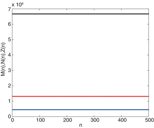
Example 2.3.

In this example, all parameter values are taken in [1] as $r_1=0.18{\mathrm{day}}^{-1}$, $r_2=0.0245{\mathrm{day}}^{-1}$, $k_1=5\times {10}^6\mathrm{cells}$, $k_2=1\times {10}^7\mathrm{cells}$, $\beta =6.2\times {10}^{-9}{\mathrm{cells}}^{-1}{\mathrm{day}}^{-1}$, ${\alpha }_2=3.422\times {10}^{-10}{\mathrm{cells}}^{-1}{\mathrm{day}}^{-1}$, $d_1=0.0412{\mathrm{day}}^{-1}$, except ${\alpha }_1$. It can be seen that under the conditions given in Theorem 2.2 and using initial conditions $M\left(0\right)=4.53941\times {10}^5$, $N\left(0\right)=1.3158\times {10}^6$ and $Z\left(0\right)=6.67022\times {10}^6$, the equilibrium point $\overline{E}=(\overline{M},\overline{N},\overline{Z})=(4.53941\times {10}^5,1.3158\times {10}^6,6.67022\times {10}^6)$ is local asymptotically stable where blue, red and black graphs represent $M\left(n\right)$, $N\left(n\right)$ and $Z\left(n\right)$ population densities, respectively (see Figure 1).

Figure 1. Graph of the iteration solution of $M\left(n\right)$, $N\left(n\right)$ and $Z\left(n\right)$,where $\alpha =1.24379\times {10}^{-7}$.

Using the parameter values given in Example 2.3, positive equilibrium point $\overline{E}=(4.53941\times {10}^5,1.3158\times {10}^6,6.67022\times {10}^6)$ is obtained under the conditions $\beta >4.2911\times {10}^{-9}$ and ${\alpha }_1<1.35777\times {10}^{-7}$ which are exactly the same as in those of Banerjee and Sarkar [1]. In addition, our stability results can be compared numerically with that of work [1]. Although in their delayed system local stability condition on parameter β is $\beta >4.2911\times {10}^{-9}$, we have $4.2911\times {10}^{-9}<\beta <1.0429\times {10}^{-7}$ which is obtained from Theorem 2.2. In addition at the present study, the condition on ${\alpha }_1$ is ${\alpha }_1<1.35777\times {10}^{-7}$, but this condition is determined as ${\alpha }_1<1.26004\times {10}^{-7}$ in study [1] under the set of our parameter values. These results indicate that there is a little differences between their and our stability conditions.

Theorem 2.4.

Let $A_1=r_1-{\alpha }_{1}N\left(n\right),$ $A_2=r_2-\beta N\left(n\right)$ and $A_3=\beta Z\left(n\right)-d_1-{\alpha }_{2}M\left(n\right)$. Suppose that the conditions of Theorem 2.2 hold and $\begin{array}{rl}& \left(a_1\right)N\left(n\right)<\frac{r_1}{{\alpha }_1}and\overline{M}<\frac{A_1(1+\exp (-A_1\left)\right)}{2r_1{K}_1\exp (-A_1)}forM\left(n\right)\in \left(0,\frac{2\overline{M}\exp (-A_1)}{1+\exp (-A_1)}\right),\\ & \left(a_2\right)N\left(n\right)>\frac{r_1}{{\alpha }_1}and\overline{M}>\frac{-A_1(1+\exp (-A_1\left)\right)}{2r_1{K}_1(\exp (-A_1)-1)}forM\left(n\right)\in \left(\frac{2\overline{M}\exp (-A_1)}{1+\exp (-A_1)},2\overline{M}\right),\\ & \left(a_3\right)N\left(n\right)>\frac{r_1}{{\alpha }_1}forM\left(n\right)\in (2\overline{M},\mathrm{\infty }),\\ & \left(b_1\right)A_3>0forN\left(n\right)\in \left(0,\frac{2\overline{N}}{1+\exp \left(A_3\right)}\right),\\ & \left(b_2\right)A_3<0forN\left(n\right)\in \left(\frac{2\overline{N}}{1+\exp \left(A_3\right)},\mathrm{\infty }\right),\\ & \left(c_1\right)N\left(n\right)<\frac{r_2}{\beta }and\overline{Z}<\frac{A_2(1+\exp (-A_2\left)\right)}{2r_2{K}_2\exp (-A_2)}forZ\left(n\right)\in \left(0,\frac{2\overline{Z}\exp (-A_2)}{1+\exp (-A_2)}\right),\\ & \left(c_2\right)N\left(n\right)>\frac{r_2}{\beta }and\overline{Z}>\frac{-A_2(1+\exp (-A_2\left)\right)}{2r_2{K}_2(\exp (-A_2)-1)}forZ\left(n\right)\in \left(\frac{2\overline{Z}\exp (-A_2)}{1+\exp (-A_2)},2\overline{Z}\right),\\ & \left(c_3\right)N\left(n\right)>\frac{r_2}{\beta }forZ\left(n\right)\in (2\overline{Z},\mathrm{\infty }).\end{array}$

Then the positive equilibrium point of system (7(7) $\begin{array}{rl}M(n+1)& =\frac{M\left(n\right)(r_1-{\alpha }_{1}N(n\left)\right)}{r_1{K}_{1}M\left(n\right)+(r_1-{\alpha }_{1}N(n)-r_1{K}_{1}M(n\left)\right)\exp (-(r_1-{\alpha }_{1}N\left(n\right)\left)\right)},\\ N(n+1)& =N\left(n\right)\exp \left(\beta Z\right(n)-d_1-{\alpha }_{2}M(n\left)\right),\\ Z(n+1)& =\frac{Z\left(n\right)(r_2-\beta N(n\left)\right)}{r_2{K}_{2}Z\left(n\right)+(r_2-\beta N(n)-r_2{K}_{2}Z(n\left)\right)\exp (-(r_2-\beta N\left(n\right)\left)\right)},\end{array}$(7) ) is global asymptotically stable.

Proof.

Let $\overline{E}=(\overline{M},\overline{N},\overline{Z})$ is positive equilibrium point system (7(7) $\begin{array}{rl}M(n+1)& =\frac{M\left(n\right)(r_1-{\alpha }_{1}N(n\left)\right)}{r_1{K}_{1}M\left(n\right)+(r_1-{\alpha }_{1}N(n)-r_1{K}_{1}M(n\left)\right)\exp (-(r_1-{\alpha }_{1}N\left(n\right)\left)\right)},\\ N(n+1)& =N\left(n\right)\exp \left(\beta Z\right(n)-d_1-{\alpha }_{2}M(n\left)\right),\\ Z(n+1)& =\frac{Z\left(n\right)(r_2-\beta N(n\left)\right)}{r_2{K}_{2}Z\left(n\right)+(r_2-\beta N(n)-r_2{K}_{2}Z(n\left)\right)\exp (-(r_2-\beta N\left(n\right)\left)\right)},\end{array}$(7) ) and we consider a Lyapunov function $V\left(n\right)$ defined by $V\left(n\right)=\left(E\right(n)-\overline{E}{)}^2,n=0,1,2,\dots$ The change along the solutions of the system is $\mathrm{\Delta }V\left(n\right)=V(n+1)-V\left(n\right)=\left(E\right(n+1)-E(n\left)\right)\left(E\right(n+1)+E(n)-2\overline{E}).$

From the first equation in (7(7) $\begin{array}{rl}M(n+1)& =\frac{M\left(n\right)(r_1-{\alpha }_{1}N(n\left)\right)}{r_1{K}_{1}M\left(n\right)+(r_1-{\alpha }_{1}N(n)-r_1{K}_{1}M(n\left)\right)\exp (-(r_1-{\alpha }_{1}N\left(n\right)\left)\right)},\\ N(n+1)& =N\left(n\right)\exp \left(\beta Z\right(n)-d_1-{\alpha }_{2}M(n\left)\right),\\ Z(n+1)& =\frac{Z\left(n\right)(r_2-\beta N(n\left)\right)}{r_2{K}_{2}Z\left(n\right)+(r_2-\beta N(n)-r_2{K}_{2}Z(n\left)\right)\exp (-(r_2-\beta N\left(n\right)\left)\right)},\end{array}$(7) ), we get $\begin{array}{rl}\mathrm{\Delta }{V}_1\left(n\right)& =\left(M\right(n+1)-M(n\left)\right)\left(M\right(n+1)+M(n)-2\overline{M})\\ & =M\left(n\right)\left(\right(A_1-r_1{K}_{1}M\left(n\right)\left)\right(1-\exp (-A_1)\left)\right)\left(A_1\right(M\left(n\right)-\overline{M}\exp (-A_1)\\ & +\exp (-A_1)\left(M\right(n)-\overline{M}))+r_1{K}_{1}M(n\left)\right(M\left(n\right)-2\overline{M}\left)\right(1-\exp (-A_1)\left)\right).\end{array}$

For each assumption $\left(a_1\right)$, $\left(a_2\right)$ and $\left(a_3\right)$, we have $\mathrm{\Delta }{V}_1\left(n\right)<0$ which implies $\underset{n\to \mathrm{\infty }}{lim}M\left(n\right)=\overline{M}$. Additionally, we hold $\begin{array}{rl}\mathrm{\Delta }{V}_2\left(n\right)& =\left(N\right(n+1)-N(n\left)\right)\left(N\right(n+1)+N(n)-2\overline{N})\\ & =N\left(n\right)(\exp (A_3)-1)\left(N\right(n)\exp (A_3)+N(n)-2\overline{N})<0\end{array}$ for each assumption $\left(b_1\right)$ and $\left(b_2\right)$ which follows $\underset{n\to \mathrm{\infty }}{lim}N\left(n\right)=\overline{N}$. Similarly, it can be shown that $\mathrm{\Delta }{V}_3\left(n\right)=\left(Z\right(n+1)-Z(n\left)\right)\left(Z\right(n+1)+Z(n)-2\overline{Z})<0$ under the assumptions $\left(c_1\right)$, $\left(c_2\right)$ and $\left(c_3\right)$. As a result, we obtain $\mathrm{\Delta }V\left(n\right)=(\mathrm{\Delta }{V}_1\left(n\right),\mathrm{\Delta }{V}_2\left(n\right),\mathrm{\Delta }{V}_3\left(n\right))<0$.

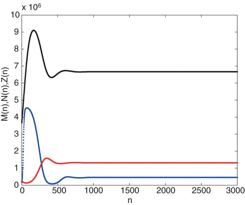
Example 2.5.

Considering conditions of Theorem 2.4, we can use the parameter values in Example 2.3 and initial conditions $M\left(0\right)=1.53\times {10}^5$, $N\left(0\right)=2.31\times {10}^5$ and $Z\left(0\right)=3.67\times {10}^6$. The graph of the first 3000 iterations of system (7(7) $\begin{array}{rl}M(n+1)& =\frac{M\left(n\right)(r_1-{\alpha }_{1}N(n\left)\right)}{r_1{K}_{1}M\left(n\right)+(r_1-{\alpha }_{1}N(n)-r_1{K}_{1}M(n\left)\right)\exp (-(r_1-{\alpha }_{1}N\left(n\right)\left)\right)},\\ N(n+1)& =N\left(n\right)\exp \left(\beta Z\right(n)-d_1-{\alpha }_{2}M(n\left)\right),\\ Z(n+1)& =\frac{Z\left(n\right)(r_2-\beta N(n\left)\right)}{r_2{K}_{2}Z\left(n\right)+(r_2-\beta N(n)-r_2{K}_{2}Z(n\left)\right)\exp (-(r_2-\beta N\left(n\right)\left)\right)},\end{array}$(7) ) is given in Figure 2, where blue, red and black graphs represent $M\left(n\right)$, $N\left(n\right)$ and $Z\left(n\right)$ population densities, respectively. It can be shown that under the conditions given in Theorem 2.4 the positive equilibrium point is global asymptotically stable.

Figure 2. Graph of the iteration solution of $M\left(n\right)$, $N\left(n\right)$ and $Z\left(n\right)$, where $\alpha =1.24379\times {10}^{-7}$. Parameter values are taken Example 2.3.

3. Neimark-Sacker bifurcation analysis

The Neimark-Sacker bifurcation is extremely important in the context of discrete biological models, where one observes periodic solutions corresponding to a closed invariant curve (that is a limit cycle) in the phase space. For this bifurcation, characteristic equation has a pair of complex conjugate eigenvalues on the unit circle and all other eigenvalues are inside the circle.

To study Neimark-Sacker bifurcation as in the work of Banerjee and Sarkar [1], we choose parameter β as a bifurcation parameter. We can plot dominant eigenvalues of the system against to β to get some information about stability of the system according to changing of this parameter. Until β reaches a critical value, the norms are less than 1 and the system is stable. If β is increased beyond this critical value, the norms will be greater than 1 and stability of the system switches to unstable situation (see Figure 3). We can also determine this critical value of β by using the Schur–Cohn criterion that is given as follows.

Figure 3. Graph of the $(\beta ,\mid \lambda \mid )$. Parameter set is taken from Example 2.3.

Theorem 3.1

[7]

A pair of complex conjugate roots of equation (17) $p\left(\lambda \right)={\lambda }^3+p_2{\lambda }^2+p_1\lambda +p_0$(17) lie on the unit circle and the other roots of equation (17(17) $p\left(\lambda \right)={\lambda }^3+p_2{\lambda }^2+p_1\lambda +p_0$(17) ) all lie inside the unit circle if and only if

• (a) $p\left(1\right)=1+p_2+p_1+p_0>0$ and $p(-1)=1-p_2+p_1-p_0>0,$

• (b) $D_2^{+}=1+p_1-p_0^2-p_0{p}_2>0,$

• (c) $D_2^{-}=1-p_1-p_0^2+p_0{p}_2=0$.

Now, we return matrix ${\mathbf{J}}_{\mathbf{F}}\left(\overline{E}\right)$ to determine bifurcation point of system (7(7) $\begin{array}{rl}M(n+1)& =\frac{M\left(n\right)(r_1-{\alpha }_{1}N(n\left)\right)}{r_1{K}_{1}M\left(n\right)+(r_1-{\alpha }_{1}N(n)-r_1{K}_{1}M(n\left)\right)\exp (-(r_1-{\alpha }_{1}N\left(n\right)\left)\right)},\\ N(n+1)& =N\left(n\right)\exp \left(\beta Z\right(n)-d_1-{\alpha }_{2}M(n\left)\right),\\ Z(n+1)& =\frac{Z\left(n\right)(r_2-\beta N(n\left)\right)}{r_2{K}_{2}Z\left(n\right)+(r_2-\beta N(n)-r_2{K}_{2}Z(n\left)\right)\exp (-(r_2-\beta N\left(n\right)\left)\right)},\end{array}$(7) ). Computations give us that the exact characteristic polynomial (there is no assumption on the matrix) of matrix ${\mathbf{J}}_{\mathbf{F}}\left(\overline{E}\right)$ is the form Equation (17(17) $p\left(\lambda \right)={\lambda }^3+p_2{\lambda }^2+p_1\lambda +p_0$(17) ) where $\begin{array}{rl}{p}_2& =-1-\exp (-K_1{r}_1\overline{M})-\exp (-K_2{r}_2\overline{Z}),\\ p_1& =\exp (-K_1{r}_1\overline{M})+\exp (-K_2{r}_2\overline{Z})+\exp (-K_1{r}_1\overline{M}-K_2{r}_2\overline{Z})\\ & +\overline{N}\frac{{\beta }^2{K}_1{r}_1(1-\exp (-K_2{r}_2\overline{Z}\left)\right)-K_2{r}_2{\alpha }_1{\alpha }_2(1-\exp (-K_1{r}_1\overline{M}\left)\right)}{K_1{r}_1{K}_2{r}_2},\\ p_0& =-\exp (-K_1{r}_1\overline{M}-K_2{r}_2\overline{Z})-\frac{{\beta }^2\overline{N}}{K_2{r}_2}\exp (-K_1{r}_1\overline{M})(1-\exp (-K_2{r}_2\overline{Z}\left)\right)\\ & +\frac{{\alpha }_1{\alpha }_2}{K_1{r}_1}\overline{N}\exp (-K_2{r}_2\overline{Z})(1-\exp (-K_1{r}_1\overline{M}\left)\right).\end{array}$

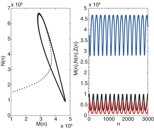
Example 3.2.

Solving equation c of Theorem 3.1, we have $\overline{\beta }=7.95907\times {10}^{-8}$. Furthermore, we have also $p\left(1\right)=0.000132031>0$, $p(-1)=7.46124>0$ and $D_2^{+}=0.500887>0$ for $\overline{\beta }$. Figure 4 shows that $\overline{\beta }$ is the Neimark-Sacker bifurcation point of the system with eigenvalues ${\lambda }_1=0.865769$, $|{\lambda }_{2,3}|=|0.999508\pm 0.0313588i|=1$, where blue, red and black graphs represent $M\left(n\right)$, $N\left(n\right)$ and $Z\left(n\right)$ population densities, respectively.

Figure 4. Graph of Neimark-Sacker bifurcation of system (7(7) $\begin{array}{rl}M(n+1)& =\frac{M\left(n\right)(r_1-{\alpha }_{1}N(n\left)\right)}{r_1{K}_{1}M\left(n\right)+(r_1-{\alpha }_{1}N(n)-r_1{K}_{1}M(n\left)\right)\exp (-(r_1-{\alpha }_{1}N\left(n\right)\left)\right)},\\ N(n+1)& =N\left(n\right)\exp \left(\beta Z\right(n)-d_1-{\alpha }_{2}M(n\left)\right),\\ Z(n+1)& =\frac{Z\left(n\right)(r_2-\beta N(n\left)\right)}{r_2{K}_{2}Z\left(n\right)+(r_2-\beta N(n)-r_2{K}_{2}Z(n\left)\right)\exp (-(r_2-\beta N\left(n\right)\left)\right)},\end{array}$(7) ) for $\beta =7.95907\times {10}^{-8}$, where $M\left(0\right)=1\times {10}^6$, $N\left(0\right)=1.5\times {10}^5$, $Z\left(0\right)=9\times {10}^5$. The other parameters are taken Example 2.3.

4. Result and discussion

In this paper, we have modified the tumour growth model proposed in [1] using system of differential equation with piecewise constant arguments that includes both discrete and continuous time for the populations. Some theoretical results for the boundedness, local and global stability of the system are obtained. The parameter values are selected from the study [1] which are obtained results of experiment on the dynamics of growth of highly malignant B Lymphoma Leukemic cells in the spleen of chimeric mice [1]. We observe that the parameter ${\alpha }_1$ (decay rate of tumour cells) and parameter β (conversion rate from resting to hunting cells) play a key role to control the unlimited growth of tumour cells so as to control the oscillations of the tumour cells. Local stability analysis shows that if the parameter ${\alpha }_1$ is less than a threshold value $1.35777\times {10}^{-7}$ and parameter β is in interval $4.2911\times {10}^{-9}<\beta <1.0429\times {10}^{-7}$, then tumour, hunting and resting cell coexist as a stable steady state (Figure 1). In addition, global stability analysis implies that the stability of the system with local stability conditions does not depend on initial conditions of the tumour, hunting and resting populations (Figure 2).

Figure 5. Graph of iteration solution of the system for $\beta =2\times {10}^{-8}$. The other parameters and initial conditions are the same as Figure 4.

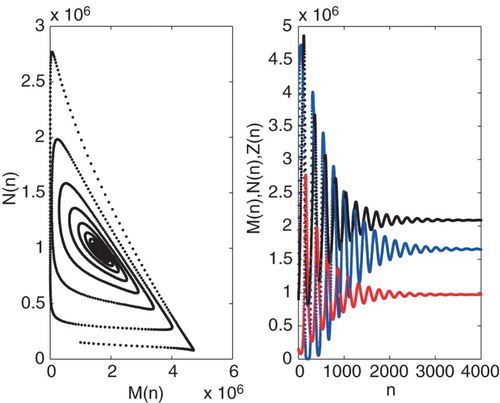
Figure 6. Graph of iteration solution of the system for $\beta =1.5\times {10}^{-7}$. The other parameters and initial conditions are the same as Figure 4.

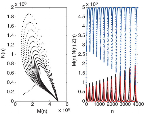
Figure 7. Graph of the iteration solution of $M\left(n\right)$, $N\left(n\right)$ and $Z\left(n\right)$, where $\alpha =2.74379\times {10}^{-6}$. The other parameters are the same as Figure 6.

The Neimark-Sacker bifurcation is the discrete analogue of the Hopf bifurcation that occurs in continuous systems such as in [1]. In their study, a stable limit cycle constructed by Hopf bifurcation is formed around the equilibrium point which depends on changing the parameter τ and β. This result is also valid for system (7(7) $\begin{array}{rl}M(n+1)& =\frac{M\left(n\right)(r_1-{\alpha }_{1}N(n\left)\right)}{r_1{K}_{1}M\left(n\right)+(r_1-{\alpha }_{1}N(n)-r_1{K}_{1}M(n\left)\right)\exp (-(r_1-{\alpha }_{1}N\left(n\right)\left)\right)},\\ N(n+1)& =N\left(n\right)\exp \left(\beta Z\right(n)-d_1-{\alpha }_{2}M(n\left)\right),\\ Z(n+1)& =\frac{Z\left(n\right)(r_2-\beta N(n\left)\right)}{r_2{K}_{2}Z\left(n\right)+(r_2-\beta N(n)-r_2{K}_{2}Z(n\left)\right)\exp (-(r_2-\beta N\left(n\right)\left)\right)},\end{array}$(7) ). As seen in Figure 4, stable periodic solutions occur at Neimark-Sacker bifurcation point (that is $\overline{\beta }=7.95907\times {10}^{-8}$) as a result of stable limit cycle. The existence of periodic solutions is relevant in tumour growth models. It means that the tumour population may oscillate around a equilibrium point even in the absence of any treatment. Such a phenomenon, which is known as Jeff 's Phenomenon, has been observed clinically [1]. When the value of parameter β is less than $\overline{\beta }$ which falls in stable region (seeFigure 3), the solution of system (7(7) $\begin{array}{rl}M(n+1)& =\frac{M\left(n\right)(r_1-{\alpha }_{1}N(n\left)\right)}{r_1{K}_{1}M\left(n\right)+(r_1-{\alpha }_{1}N(n)-r_1{K}_{1}M(n\left)\right)\exp (-(r_1-{\alpha }_{1}N\left(n\right)\left)\right)},\\ N(n+1)& =N\left(n\right)\exp \left(\beta Z\right(n)-d_1-{\alpha }_{2}M(n\left)\right),\\ Z(n+1)& =\frac{Z\left(n\right)(r_2-\beta N(n\left)\right)}{r_2{K}_{2}Z\left(n\right)+(r_2-\beta N(n)-r_2{K}_{2}Z(n\left)\right)\exp (-(r_2-\beta N\left(n\right)\left)\right)},\end{array}$(7) ) has damped oscillation and the positive equilibrium point is local asymptotically stable (see Figure 5 for $\beta =2\times {10}^{-8}$). This implies that tumour, hunting and resting cell coexist as a stable steady state as a result of competition, namely tumour dormancy. If the value of parameter β is greater than $\overline{\beta }$ which falls in unstable region (see Figure 3), the system has unstable oscillation and the positive equilibrium point is unstable (see Figure 6 for $\beta =1.5\times {10}^{-7}$). 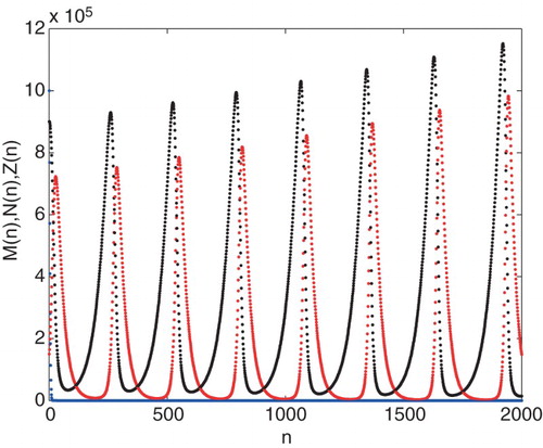In this situation, tumour cells have growing oscillation with very high amplitude. We also investigate the dynamic behaviour of the system in the region ($\beta >\overline{\beta }$) where the system exhibits unstable oscillation. In this region, decay rate of tumour cells ${\alpha }_1$ plays an important role in controlling tumour cells growth. As the parameter ${\alpha }_1$ is increased in this region, the population size of tumour cells can be constrained to null values namely tumour-free steady state where the tumour cells are eliminated by hunting cells. Therefore, it is possible to reach the tumour-free steady state by increasing the parameter ${\alpha }_1$ (Figure 7).

When our theoretical and numerical results are compared with that of work [1], we obtain a good compatibility. Hence, differential equations with piecewise constant arguments may be used to approximate delay differential equations that contain discrete delays [3].

Disclosure statement

No potential conflict of interest was reported by the authors.

References

- S. Banerjee and R.R. Sarkar, Delay-induced model for tumor-immune interaction and control of malignant tumor growth, Biosystems 91 (2008), pp. 268–288. doi: 10.1016/j.biosystems.2007.10.002
- F. Bozkurt, Modeling a tumor growth with piecewise constant arguments, Discret. Dyn. Nat. Soc. (2013), Article ID 841764.
- K.L. Cooke and I. Györi, Numerical approximation of the solutions of delay differential equations on an infinite interval using piecewise constant arguments, Comput. Math. Appl. 28 (1994), pp. 81–92. doi: 10.1016/0898-1221(94)00095-6
- K. Gopalsamy and P. Liu, Persistence and global stability in a population model, J. Math. Anal. Appl. 224 (1998), pp. 59–80. doi: 10.1006/jmaa.1998.5984
- F. Gurcan and F. Bozkurt, Global stability in a population model with piecewise constant arguments, J. Math. Anal. Appl. 360 (2009), pp. 334–342. doi: 10.1016/j.jmaa.2009.06.058
- S. Kartal, Mathematical modeling and analysis of tumor-immune system interaction by using Lotka-Volterra predator–prey like model with piecewise constant arguments, PEN 2 (2014), pp. 7–12.
- X. Li, C. Mou, W. Niu, and D. Wang, Stability analysis for discrete biological models using algebraic methods, Math. Comput. Sci. 5 (2011), pp. 247–262. doi: 10.1007/s11786-011-0096-z
- P. Liu and K. Gopalsamy, Global stability and chaos in a population model with piecewise constant arguments, Appl. Math.Comput. 101 (1999), pp. 63–88. doi: 10.1016/S0096-3003(98)00037-X
- R.M. May, Biological populations obeying difference equations: Stable points, stable cycles and chaos, J. Theor. Biol. 51 (1975), pp. 511–524. doi: 10.1016/0022-5193(75)90078-8
- R.M. May and G.F. Oster, Bifurcations and dynamic complexity in simple ecological models, Am. Nat. 110 (1976), pp. 573–599. doi: 10.1086/283092
- Y. Muroya, Persistence, contractivity and global stability in logistic equations with piecewise constant delays, J. Math. Anal. Appl. 270 (2002), pp. 602–635. doi: 10.1016/S0022-247X(02)00095-1
- Y. Muroya, New contractivity condition in a population model with piecewise constant arguments, J. Math. Anal. Appl. 346 (2008), pp. 65–81. doi: 10.1016/j.jmaa.2008.05.025
- I. Ozturk and F. Bozkurt, Stability analysis of a population model with piecewise constant arguments, Nonlinear Anal. Real. 12 (2011), pp. 1532–1545. doi: 10.1016/j.nonrwa.2010.10.011
- I. Ozturk, F. Bozkurt, and F. Gurcan, Stability analysis of a mathematical model in a microcosm with piecewise constant arguments, Math. Biosci. 240 (2012), pp. 85–91. doi: 10.1016/j.mbs.2012.08.003
- J.W.-H . So and J.S. Yu, Global stability in a logistic equation with piecewise constant arguments, Hokkaido Math. J. 24 (1995), pp. 269–286. doi: 10.14492/hokmj/1380892595
- K. Uesugi, Y. Muroya, and E. Ishiwata, On the global attractivity for a logistic equation with piecewise constant arguments, J. Math. Anal. Appl. 294 (2004), pp. 560–580. doi: 10.1016/j.jmaa.2004.02.031