
 ?Mathematical formulae have been encoded as MathML and are displayed in this HTML version using MathJax in order to improve their display. Uncheck the box to turn MathJax off. This feature requires Javascript. Click on a formula to zoom.
Abstract
We illustrate the use of statistical tools (asymptotic theories of standard error quantification using appropriate statistical models, bootstrapping, and model comparison techniques) in addition to sensitivity analysis that may be employed to determine the information content in data sets. We do this in the context of recent models [S. Prigent, A. Ballesta, F. Charles, N. Lenuzza, P. Gabriel, L.M. Tine, H. Rezaei, and M. Doumic, An efficient kinetic model for assemblies of amyloid fibrils and its application to polyglutamine aggregation, PLoS ONE 7 (2012), e43273. doi:10.1371/journal.pone.0043273.] for nucleated polymerization in proteins, about which very little is known regarding the underlying mechanisms; thus, the methodology we develop here may be of great help to experimentalists. We conclude that the investigated data sets will support with reasonable levels of uncertainty only the estimation of the parameters related to the early steps of the aggregation process.
1. Introduction
As mathematical models become more complex with multiple states, increasing numbers of parameters need to be estimated using experimental data. Thus there is a need for critical analysis in model validation related to the reliability of parameter estimates obtained in model fitting. A recent concrete example involves previous HIV models [Citation1,Citation6] with 15 or more parameters to be estimated. In [Citation8], using recently developed parameter selectivity tools [Citation7] based on parameter sensitivity-based scores, it was shown that a number of these parameters could not be estimated with any degree of reliability. Moreover, we found that quantifiable uncertainty varies among patients depending upon the number of treatment interruptions (perturbations of therapy). This leads to a fundamental question: How much information with respect to model validation can be expected in a given data set or collection of data sets?
Here we illustrate the use of other tools: asymptotic theories (as the data sample size increases without bound) of standard error (SE) quantification using appropriate statistical models, bootstrapping (repeated sampling of synthetic data similar to the original data), and statistical (ANOVA type) model comparison techniques – these are discussed in some detail in the recent monograph [Citation11] as well as in numerous statistical texts. Such techniques are employed in addition to sensitivity theory in order to determine the information content in data sets. We pursue this in the context of recent models [Citation25] for nucleated polymerization in proteins.
After briefly outlining the biological context of amyloid formation, we describe the model in Section 2. In Section 3, we investigate the statistical model to be used with our noisy data. This is a necessary step in order to use the correct error model in our generalized least-squares (GLS) minimization. This also reveals information on our experimental observation process. Once we have found parameters which allow a reasonable fit, we determine the confidence we may have in our estimation procedures. We do this in Section 4, using both the condition number of the covariance matrix and a sensitivity analysis. This reveals a smaller number of parameters (than those estimated in [Citation25]) to be reasonably sensitive to the data sets, whereas others do not really affect the quality of the fits to our data. To further support our sensitivity findings, we then apply a bootstrapping analysis in Section 5. We are lead to four main parameters and compare their resulting errors with the asymptotic confidence intervals of Section 4. Finally, in Section 6, we carry out model comparison tests [Citation3,Citation5,Citation11] as used in [Citation10], and these lead us to select three parameters out of the nine original ones estimated in [Citation25] that can be reliably estimated.
1.1. Protein polymerization
It is now known that several neurodegenerative disorders, including Alzheimer's disease, Huntington's disease, and Prion diseases, for example, mad cow, are related to aggregations of proteins presenting an abnormal folding. These protein aggregates are called amyloids and have become a focus of modelling efforts in recent years [Citation12,Citation25,Citation29–31]. One of the main challenges in this field is to understand the key aggregation mechanisms, both qualitatively and quantitatively. In order to test our methodology on a relatively simple case, we focus here on polyglutamine (PolyQ)-containing proteins. This was also the case study chosen to illustrate the fairly general ordinary differential equation (ODE)–partial differential equation (PDE) model proposed in [Citation25]; the reason for our choice is that, as shown in [Citation25], the polymerization mechanisms prove to be simpler for PolyQ aggregation than for other types of proteins ( e.g. PrP) [Citation21]. To understand data sets from experiments carried out by Human Rezaei and his team at INRA (Virologie et Immunologie Moleculaires) [Citation25], we adapt the general model to this context. The data sets (DS1–DS4) of interest to us here are depicted in Figure and record the evolution of normalized total polymerized mass in time.
Figure 1. The data sets of interest from [Citation9,Citation25]. The total polymerized mass is measured by Thioflavin T (ThT), which is one of the most common experimental tools for in vitro protein polymerization [Citation25,Citation29]. (available in colour online)
![Figure 1. The data sets of interest from [Citation9,Citation25]. The total polymerized mass is measured by Thioflavin T (ThT), which is one of the most common experimental tools for in vitro protein polymerization [Citation25,Citation29]. (available in colour online)](/cms/asset/9e065c6a-b2d5-4983-ac1f-8a0ef4d0931f/tjbd_a_1050465_f0001_c.jpg)
In [Citation25] and a subsequent effort in [Citation9], the authors sought to investigate several questions including (i) understanding the key polymerization mechanisms, (ii) how to numerically approximate the model, and (iii) how to select parameters and calibrate the model. Here we briefly summarize results related to (ii) and focus primarily on (iii).
2. The model
2.1. Original ODE model
We briefly outline the model that is the same as that of [Citation25]. Let be the main variables of interest consisting, respectively, of concentrations of the normal proteins that we will call monomers (basic subunits that are repeated in a chainlike fashion), of the monomeric proteins presenting an abnormal configuration that we will call conformers, and of the i-polymers made of i aggregated abnormal proteins. The following comprise the fundamental dynamics modelled in [Citation25] which the interested reader may consult for further details:
Monomer–conformer exchange:
. This represents the spontaneous formation of an active form of the monomer, denoted here
Nucleation:
Polymerization by conformer addition:
Other reactions like fragmentation and coalescence are negligible for the case of PolyQ-containing proteins (see [Citation25] for experimental justification).
The law of mass action in the deterministic framework (see [Citation5,Citation27] and the numerous references therein) translates into the ODE
. Using these basic ideas we obtain the infinite system of ODEs studied in [Citation25]
(1)
(1)
(2)
(2)
(3)
(3)
(4)
(4) with initial conditions
and the mass balance equation
The experiments of interest to us measure the a-dimensional total polymerized mass, or
Madim which is given by
2.2. An approximate PDE system and the associated forward problem
Amyloid formations are characterized by very long polymers (a fibril may contain up to monomer units). A PDE version of the standard model, where a continuous variable x approximates the discrete sizes i, is thus a reasonable approximation for large amyloid polymers. However, for small polymer sizes this resulting continuum approximation does not work very well. Thus, we take a ‘hybrid approach’ of retaining the ODE for smaller sizes and using the PDE for larger ones [Citation9].
We define a small parameter , and let
with
being the average polymer size defined by
Then after definition of dimensionless quantities
we may obtain a PDE to replace the infinite ODE system. Rigorous derivations of such continuous integro-PDE models may be found in [Citation22] for coagulation-fragmentation equations, in [Citation15] for the limit of the so-called Becker– Döring system (polymerization and depolymerization reactions are the only reactions considered) towards its continuous limit called the Lifshitz–Slyozov model, and in [Citation19] for the growth-fragmentation ‘Prion Model’. A formal derivation for a full model, also including nucleation, is carried out in [Citation25].
Let . We then use the approximation
(5)
(5)
(6)
(6)
(7)
(7)
(8)
(8)
with initial conditions
and the boundary condition
Here we have passed to the continuous representations for chain lengths larger than
.
Then an assumed mass balance equation becomes
In [Citation9], we considered requirements for a good discretization scheme including the following: (i) it should conserve the a-dimensional total polymerized mass (Madim), (ii) it should be fast, and most importantly, (iii) it should be accurate.
To ensure the conservation of mass, we replace the ODE for by the mass conservation equation and obtain
(9)
(9)
(10)
(10)
with initial and boundary conditions as before.
We developed methodology for forward solutions in [Citation9]. We first point out that the desired spatial computational domain is very large as determined by the maximum size of observed polymers, with range up to . The peak in the distribution is at the left side of the domain of interest; for larger polymer sizes, the distribution is almost linearly decreasing.
Based on these and other considerations discussed in [Citation9], the PDE was approximated by the Finite Volume Method (see [Citation23] for discussions of Upwind, Lax–Wendroff, and flux limiter methods) with an adaptive mesh, refined towards the smaller polymer sizes. Furthermore, we kept the ratio between the step size and the corresponding mesh element constant, that is, we used so that
. This mesh is quasi-linear in the sense of
. The resulting Upwind and Lax–Wendroff schemes are then consistent on the progressive mesh [Citation23]. For further details on these schemes including examples demonstrating convergence properties, the interested reader may consult [Citation9].
3. The inverse problem
A major question in formulating the model for use in inverse problem scenarios consists of how to best parametrically represent the polymerization parameters of Equation (Equation3
(3)
(3) ) and the function
of Equation (Equation4
(4)
(4) ) for our application. We do this in a combined piecewise continuous formulation.
For this continuous polymerization function , we use the piecewise linear representation (Figure )
In the numerical approximations, we chose
. The discrete polymerization parameters
,
, are then obtained as
Figure 2. Parametric representation for .
Following [Citation25], we chose to approximate by a function as depicted in Figure . (According to our discussions with S. Prigent, H. Rezaei and J. Torrent, other choices like a Gaussian bell curve are also possible, but as we will subsequently conclude, the presently available data will not support estimation of parameters in these representations.) Thus with this parametrization we have five more parameters
the fractions
and
in addition to the four basic parameters
to be estimated using our data sets.
Thus, we seek to estimate (with acceptable quantification of uncertainties) the nine parameters , and
(represented in parametrical form depicted above with the five additional unknowns
) that fit the data best. To do this we need an efficient discretization method as discussed above for the forward problem as well as a correct assumption on the measurement errors in the inverse problem.
3.1. Estimation of parameters
We make some standard statistical assumptions (see [Citation5,Citation11,Citation17,Citation28]) underlying our inverse problem formulations.
Assume that there exists a true or nominal set of parameter
Let
Denote as the estimated parameter for
. The inverse problem is based on statistical assumptions on the observation error in the data.
If we assume an absolute error data model, then data points are taken with equal importance. This is represented by observations (here is a realization of the error process
)
(11)
(11)
On the other hand, if one assumes some type of relative error data model, then the error is proportional in some sense to the measured polymerized mass. This can be represented by observations of the form
(12)
(12)
Absolute model error formulations dictate we use ordinary least-squares (OLS) inverse problem [Citation5,Citation11] given by
(13)
(13) while for relative error models one should use inverse problem formulations with
GLS cost functional
(14)
(14)
3.1.1. The residual plots.
To obtain a best statistical model, we used residual plots (see [Citation5,Citation11] for more details) with residuals given by
To illustrate what we are seeking for our data sets, we first used simulated relative error data (simulated data for ), then carried out the inverse problems for both a relative error cost functional (i.e.
) and an OLS cost functional (i.e.
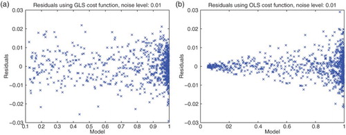
). We then plotted the corresponding residuals vs. time and also residuals vs. the model values. The first plots are related to the correctness of our assumption of independency and identical distributions i.i.d. for the data, whereas the second plots contain information as to the correctness of the form of our proposed statistical model (Figures and ).
Figure 3. Plots with simulated data: (a) correct cost function vs. time ; (b) incorrect cost function vs. time
.
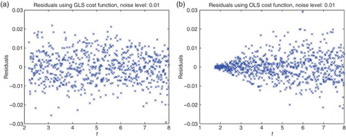
Figure 4. Plots with simulated data: (a) correct cost function vs. model ; (b) incorrect cost function vs. model
.
3.2. Statistical models of noise
We next carried out similar inverse problems with data set (DS) 4 of our experimental data collection. We first used DS4 on the interval . Based on some earlier calculations we also chose the nucleation index
for all our subsequent calculations. The residual plots given in Figures and suggest strongly that neither of the first attempts of assumed statistical models and corresponding cost functionals (absolute error and OLS or relative error with
and simple GLS) are correct.
Figure 5. (a) (Madim) with OLS; (b) residuals vs. model: OLS.
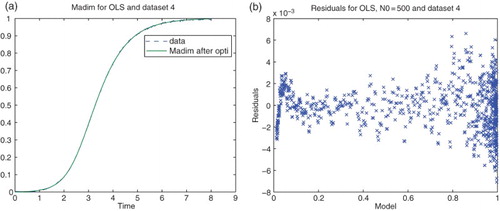
Figure 6. (a) with GLS,
; (b) residuals vs. model: GLS.
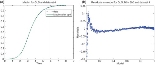
Based on these initial results and the speculation that early periods of the polymerization process may be somewhat stochastic in nature, we chose to subsequently use all the data sets on the intervals where
is the first time when
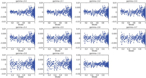
(thus 12% of the a-dimensional total polymerized mass). Moreover, we decided to use other values of γ between 0 and 1 to test DS4. Setting
, we focused on the question of the most appropriate values of γ to use in a GLS approach (again see [Citation11] for further motivation and details). We then obtained the results with DS4 depicted in Figure . Analysis of these residuals suggest that either
or
might be satisfactory for use in a GLS setting.
Figure 7. Residuals for DS4 using different values of γ.
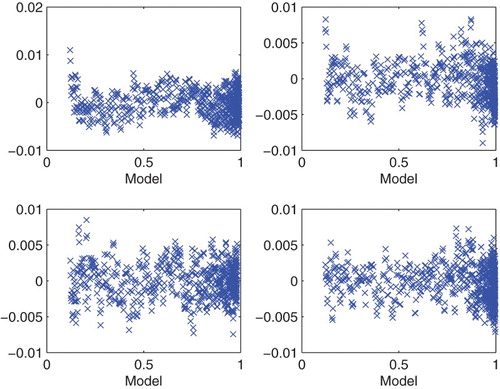
Motivated by these results, we next investigated the inverse problems for each of the four experimental data sets with initial concentration and
. We carried out the optimization over all data points with
and used the GLS method with
. The resulting graphics depicted in Figure again suggest that
is a reasonable value to use in our subsequent analysis of the PolyQ data with regard to its information content for inverse problem estimation and parameter uncertainty quantification.
Figure 8. Residuals for the four experimental data sets using .
4. SEs and asymptotic analysis
4.1. SEs for parameters using GLS
We employed first the asymptotic theory (as ) for parameter uncertainty summarized in [Citation5,Citation11,Citation17] and references therein. In the case of GLS, the associated SEs for the estimated parameters
(vector length
) are given by the following construction (for details see Chaps 3.2.5 and 3.2.6 of [Citation11]).
We may define the SEs by the formula
where the covariance matrix Σ is given by
Here
is the sensitivity matrix of size
(n being the number of data points and
being the number of estimated parameters) and W is defined by
We use the approximation of the variance
To obtain a finite SE using asymptotic theory, the matrix
thus must be invertible. In the above problem, we do indeed obtain a good fit of the curve and good residuals (for the sake of brevity, not depicted here). However, we also found that the condition number of the matrix
is
. Looking more closely at the matrix F reveals a near linear dependence between certain rows, hence the large condition number. We thus quickly reach the following conclusions:
We obtain a set of parameters for which the model fits well, but we cannot have any reasonable confidence in them using the asymptotic theories from statistics ( e.g. see the references given above).
We suspect that it may not be possible to obtain sufficient information from our data set curves to estimate all nine parameters with a high degree of confidence. This is based on our calculations with the corresponding Fisher matrices as well our prior knowledge in that the graphs depicted in Figure are very similar to Logistic or Gompertz curves. These curves can be quite well fit with parameterized models with only two or three carefully chosen parameters.
To assist in initial understanding of these issues, we consider components of the associated sensitivity matrices .
4.2. Sensitivity analysis
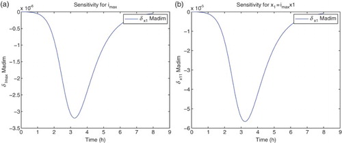
For the sensitivity analysis, we follow [Citation5,Citation11] and carry out all computations using the differential system of sensitivity equations as detailed in those references. Hereafter all our analysis will be carried out using DS4 and the best estimate obtained for the latter. We find that the model is sensitive mainly to four parameters:
. The sensitivities for the remaining parameters are on an order of magnitude of
or less. It also shows some sensitivity with respect to
. However, the parameter
appears in the model only as the factor
. The sensitivities depicted in the following use
for the nine best fit GLS parameters, that is,
for
. We note that since we use the a-dimensional quantity M in the cost functionals (OLS or GLS), it is the sensitivity of this quantity with respect to the parameters θ, rather than any relative sensitivities, that will determine changes in the cost functionals to be minimized with respect to changes in the parameters (Figures –).
Figure 9. (a) Sensitivity w.r.t. ; (b) sensitivity w.r.t.
.
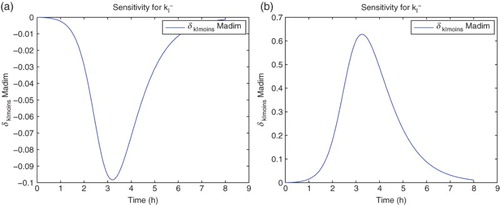
Figure 10. (a) Sensitivity w.r.t. ; (b) sensitivity w.r.t.
.
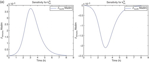
Figure 11. (a) Sensitivity w.r.t. ; (b) sensitivity w.r.t.
.
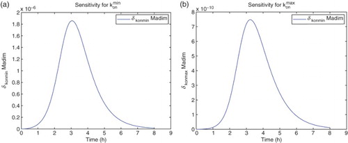
Figure 12. (a) Sensitivity w.r.t. ; (b) sensitivity w.r.t.
.

Figure 13. (a) Sensitivity w.r.t. ; (b) sensitivity w.r.t.
.
5. Sensitivity motivated inverse problems
Based on the sensitivity findings depicted above, we investigated a series of inverse problems in which we attempted to estimate an increasing number of parameters beginning first with the fundamental parameters and
. In each of these inverse problems, we attempted to ascertain uncertainty bounds for the estimated parameters using both the asymptotic theory described above and a GLS version of bootstrapping [Citation13,Citation14,Citation16,Citation18,Citation20].
A quick outline of the appropriate bootstrapping algorithm is given next.
5.1. Bootstrapping algorithm: nonconstant variance data
We suppose now that we are given experimental data from the underlying observation process
(15)
(15) where
and the
are i.i.d. with mean zero and constant variance
. Then we see that
and
, with associated corresponding realizations of
given by
A standard algorithm can be used to compute the corresponding bootstrapping estimate of
and its empirical distribution. We treat the general case for nonlinear dependence of the model output on the parameters θ. The algorithm is given as follows.
First obtain the estimate
Define the nonconstant variance standardized residuals
Set
Create a bootstrapping sample of size n using random sampling with replacement from the data (realizations) {
Create bootstrapping sample points
Obtain a new estimate
Set
We then calculate the mean, SE, and confidence intervals using the formulae
(16)
(16) where
denotes the bootstrapping estimator.
5.2. Estimation of two parameters
We first carried out estimation for the two parameters and
. We use the GLS formulation with
. We fix globally (based on previous estimations with DS4) the parameter values
Table
and used the initial guesses for the parameters given by
Table
We then used the bootstrapping algorithm and obtained the following means and SEs for which, as reported in the following, compare quite well with the asymptotic theory estimates. The corresponding distributions are shown in Figures and .
Figure 14. Two parameters estimation (,
). Bootstrapping distribution for
. We use GLS and
runs.
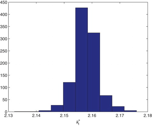
Figure 15. Two parameters estimation (,
). Bootstrapping distribution for
. We use GLS and
runs.
Table
5.3. GLS estimation of three parameters
We tried next to estimate three parameters using the GLS formulation with . Once again we fixed all the parameters describing the domain and the polymerization function
and also fixed either
or
in the corresponding inverse problems.
5.4. GLS estimation for and
We fixed values as follows:
Table
We used as initial parameter values:
Table
Table
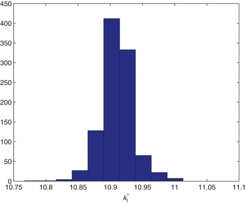
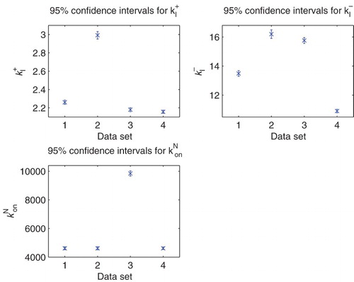
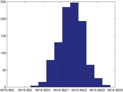
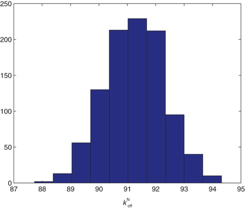
To compare these asymptotic results with bootstrapping, we carried out bootstrapping with DS4 for the estimation of ,
, and
with the same initial values as above. We then obtained the following means and SE for a run with
, in comparison to the asymptotic theory.
Figure 16. Confidence intervals.
Table
Of particular interest are the values obtained for and the bootstrapping SEs for
which are extremely small. It should be noted that the sensitivity of the model output on
is also very small. Thus one might conjecture that the iterations in the bootstrapping algorithm do not change the values of
very much and hence one observes the extremely small SE that are produced for the bootstrapping estimates (Figures –).
Figure 17. Estimation for ,
and
: bootstrapping distribution for
for GLS and
runs.
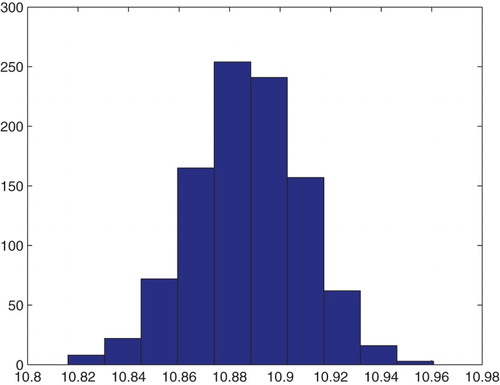
Figure 18. Estimation for ,
, and
: bootstrapping distribution for
for GLS and
runs.
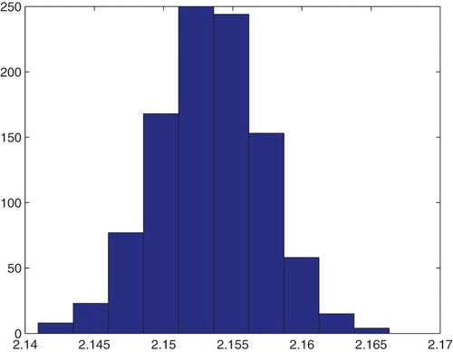
Figure 19. Estimation for ,
, and
: bootstrapping distribution for
for GLS and
runs.
5.5. GLS estimation for and
In another test, we fixed and instead estimate
(along with
and
). We use the fixed values:
Table
and the initial guesses for the parameters to be estimated given by
Table
We obtained the estimated parameters and corresponding SE.
Table
Figure 20. Three parameters estimation (,
and
): bootstrapping distribution for
. We used GLS and
runs.
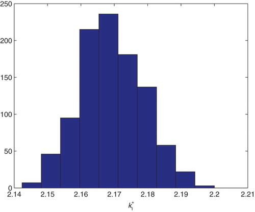
Figure 21. Three parameters estimation (,
and
): bootstrapping distribution for
. We used GLS and
runs.
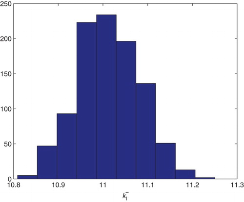
Figure 22. Three parameters estimation (,
and
): bootstrapping distribution for
. We used GLS and
runs.
Table
5.6. Estimation of four main parameters
Following the sensitivity analysis detailed above, we tried to estimate a combination of the parameters for the parameter set with
.
Parameters were fixed as follows from the original nine parameter fit:
Table
We obtained the following result for the estimation of the four parameters using the DS1–DS4. In all of them, the condition number of Fischer's information matrix κ is too large to invert. This along with the sensitivity results above strongly suggests that the data sets do not contain sufficient information to estimate four or more parameters with any degree of certainty attached to the estimates.
Table
6. Model comparison tests
A type of Residuals Sum of Squares (RSS)-based model selection criterion [Citation3,Citation5,Citation11] can be used as a tool for model comparison for certain classes of models. In particular, this is true for models such as those given in [Citation10] in which potentially extraneous mechanisms can be eliminated from the model by a simple restriction on the underlying parameter space while the form of the mathematical model remains unchanged. In other words, this methodology can be used to compare two nested mathematical models where the parameter set (this notation will be defined explicitly in Section 6.1) for the restricted model can be identified as a linearly restricted subset of the admissible parameter set
of the unrestricted model. Indeed, the RSS-based model selection criterion is a useful tool to determine whether or not certain terms in the mathematical models are important in describing the given experimental data.
6.1. Ordinary least squares
We now turn to the statistical model (Equation11(11)
(11) ), where the measurement errors are assumed to be independent and identically distributed with zero mean and constant variance
. In addition, we assume that there exists
such that the statistical model
(17)
(17) correctly describes the observation process. In other words, Equation (Equation17
(17)
(17) ) is the true model, and
is the true value of the mathematical model parameter θ.
With our assumption on measurement errors, the mathematical model parameter θ can be estimated by using the OLS method; that is, the OLS estimator of θ is obtained by solving
Here
, and the cost function
is defined as
The corresponding realization
of
is obtained by solving
where
is a realization of
(i.e.
).
As alluded to in the introduction, we might also consider a restricted version of the mathematical model in which the unknown true parameter is assumed to lie in a subset of the admissible parameter space. We assume this restriction can be written as a linear constraint,
, where
is a matrix having rank
(i.e.
is the number of constraints imposed), and
is a known vector. Thus the restricted parameter space is
Then the null and alternative hypotheses are
We may define the restricted parameter estimator as
and the corresponding realization is denoted by
. Since
, it is clear that
This fact forms the basis for a model selection criterion based upon the residual sum of squares.
Using the standard assumptions (given in detail in [Citation11]), one can establish asymptotic convergence result for the test statistics (which is a function of observations and is used to determine whether or not the null hypothesis is rejected)
where the corresponding realization
is defined as
This asymptotic convergence result is summarized in the following theorem.
Theorem 6.1
Under assumptions detailed in [Citation5,Citation11] and assuming the null hypothesis is true, then
converges in distribution
as
to a random variable U having a chi-square distribution with
degrees of freedom.
The above theorem suggests that if the sample size n is sufficiently large, then is approximately chi-square distributed with
degrees of freedom. We use this fact to determine whether or not the null hypothesis
is rejected. To do that, we choose a
significance level α (usually chosen to be 0.05) and use
tables to obtain the corresponding threshold value τ so that
. We next compute
and compare it to τ. If
, then we reject the null hypothesis
with confidence level
; otherwise, we do not reject. We emphasize that care should be taken in stating conclusions: we either reject or do not reject
at the specified level of confidence. The following table illustrates the threshold values for
with the given significance level.
Similar tables can be found in any elementary statistics text or online or calculated by some software package such as Matlab, and is given here for illustrative purposes and also for use in the examples demonstrated in the following.
6.2. Generalized least squares
The model comparison results outlined can be extended to deal with GLS problems in which measurement errors are independent with and
,
, where w is some known real-valued function with
for any t. This is achieved through rescaling the observations in accordance with their variance (as discussed in [Citation11]) so that the resulting (transformed) observations are identically distributed as well as independent.
6.3. Results for PolyQ aggregation models
We then carried out a series of model comparison tests (we again used DS4) for nested models to determine if an added parameter yields a statistically significantly improved model fit. Our null hypothesis in each case was: : The restricted model is adequate (i.e. the fit to data is not significantly improved with the model containing the additional parameter as a parameter to be estimated). We obtained the following results.
The model with estimation of
The model with estimation of
The model with estimation of
The model with estimation of
From these and the preceding results we conclude that the information content of the typical data set for the dynamics considered here will support at most three parameters estimated with reasonable confidence levels and these are the parameters
.
7. Conclusions and suggested further efforts
For the efforts reported on above we make several conclusions.
For the majority of data sets, the GLS residual plots with are random when fitted for data points
As conjectured earlier, this may be because the early formation of aggregates is somewhat stochastic in nature which is not well described by either the mathematical and/or statistical models. It appears that one needs special consideration of smaller polymer sizes. Indeed we suspect from additional discussions with our colleagues that perhaps the nucleation step might be dominated by a stochastic rather than deterministic process in the early stages (i.e. for small polymer sizes). This is a possible direction of further investigation.
Based on several different mathematical/statistical methodologies (sensitivities, asymptotic analysis, bootstrapping, and model comparison tests), the data sets we considered do not contain sufficient information for the reliable estimation of all nine parameters of interest. Indeed our findings suggest that at most three parameters can be reliably estimated with the data sets typical of those presented here, and that these parameters are . Recently related efforts [Citation2] suggest that perhaps there are experimental design questions that could be addressed to collect data that might support the more sophisticated models derived in [Citation25], especially in order to investigate information coming from different initial concentrations. Indeed, we have considered here data sets related to experiments carried out with the same initial concentration. Adapting the previously used techniques to simultaneously or successively use all the information content in data sets carried out for different initial concentration is a challenging problem (see [Citation24] for a discussion of the effect of initial concentration on nucleated polymerization).
Here we concluded that at most three parameters can be reliably estimated with the data sets investigated. The two first parameters determine the balance between the normal and abnormal protein concentrations and the third represents the stability of the nucleus against the degradation into monomeric entities. These three parameters are related to the early steps of the aggregation process, and thus we conclude that the model applied to these data sets does not provide any insight into the polymerization of larger polymers. Since this is the case, there is little motivation to modify the polymerization function
depicted in Figure until further data collection procedures are pursued. It is difficult to say whether the initiation parameters are biologically more or less interesting than other parameters in the later aggregation process. (Everything interests the biological community since very little is known with certainty.) What we can more prudently conclude is rather a negative conclusion: this type of experiments seems to be more sensitive to the ignition of the reaction than to secondary pathways, which reveals a limit, and argues for the measurement not only of the total polymerized mass but also of size distributions of fibrils if one wants to really select the proper model for self-acceleration, as for instance in [Citation26,Citation30,Citation31].
The methodology we developed here may be carried out for other types of proteins as well as related experiments, and this is of peculiar interest since the ThT measurements as studied here are the most standard method for protein aggregation. For instance, in the seminal paper [Citation29], models are proposed and fit to data; our type of analysis would complement their findings and allow one to assess the quality of these fits and how much confidence the authors can have in their conclusions. These results in turn could be combined with optimal design techniques [Citation2,Citation4,Citation11] to design more informative experiments.
Acknowledgments
The authors are most grateful to a referee whose careful reading of an earlier version of this manuscript led to substantial improvements in the final version.
Disclosure statement
No potential conflict of interest was reported by the authors.
Additional information
Funding
References
- B.M. Adams, H.T. Banks, M. Davidian, and E.S. Rosenberg, Model fitting and prediction with HIV treatment interruption data, Center for Research in Scientific Computation Technical Report CRSC-TR05-40, NC State University, October, 2005; Bull. Math. Biol. 69 (2007), pp. 563–584.
- K. Adoteye, H.T. Banks, and K.B. Flores, Optimal design of non-equilibrium experiments for genetic network interrogation, CRSC-TR14-12, N.C. State University, Raleigh, NC, September, 2014; Appl. Math. Lett. 40 (2015), pp. 84–89; DOI: 10.1016/j.aml.2014.09.013.
- H.T. Banks and B.G. Fitzpatrick, Statistical methods for model comparison in parameter estimation problems for distributed systems, J. Math. Biol. 28 (1990), pp. 501–527. doi: 10.1007/BF00164161
- H.T. Banks and K.L. Rehm, Parameter estimation in distributed systems: Optimal design, CRSC TR14-06, N.C. State University, Raleigh, NC, May, 2014; Eurasian J. Math. Comput. Appl. 2 (2014), pp. 70–79.
- H.T. Banks and H.T. Tran, Mathematical and Experimental Modeling of Physical and Biological Processes, CRC Press, Boca Raton, FL, 2009.
- H.T. Banks, M. Davidian, S. Hu, G.M. Kepler, and E.S. Rosenberg, Modeling HIV immune response and validation with clinical data, J. Biol. Dyn. 2 (2008), pp. 357–385. doi: 10.1080/17513750701813184
- H.T. Banks, A. Cintron-Arias, and F. Kappel, Parameter selection methods in inverse problem formulation, CRSC-TR10-03, N.C. State University, February, 2010, Revised, November, 2010; in Mathematical Modeling and Validation in Physiology: Application to the Cardiovascular and Respiratory Systems, J.J. Batzel, M. Bachar, and F. Kappel, eds., Lecture Notes in Mathematics Vol. 2064, Springer-Verlag, Berlin, 2013, pp. 43 – 73.
- H.T. Banks, R. Baraldi, K. Cross, K. Flores, C. McChesney, L. Poag, and E. Thorpe, Uncertainty quantification in modeling HIV viral mechanics, CRSC-TR13-16, N.C. State University, Raleigh, NC, December, 2013; Math. Biosci. Eng., to appear.
- H.T. Banks, M. Doumic, and C. Kruse, Efficient numerical schemes for nucleation-aggregation models: Early steps, CRSC-TR14-01, N.C. State University, Raleigh, NC, March, 2014.
- H.T. Banks, J.E. Banks, K. Link, J.A. Rosenheim, C. Ross, and K.A. Tillman, Model comparison tests to determine data information content, CRSC-TR14-13, N.C. State University, Raleigh, NC, October, 2014; Appl. Math. Lett. 43 (2015), pp. 10–18.
- H.T. Banks, S. Hu, and W.C. Thompson, Modeling and Inverse Problems in the Presence of Uncertainty, Taylor/Francis-Chapman/Hall-CRC Press, Boca Raton, FL, 2014.
- V. Calvez, N. Lenuzza, M. Doumic, J.-P. Deslys, F. Mouthon, and B. Perthame, Prion dynamic with size dependency – strain phenomena, J. Biol. Dyn. 4(1) (2010), pp. 28–42. doi: 10.1080/17513750902935208
- R.J. Carroll and D. Ruppert, Transformation and Weighting in Regression, Chapman & Hall, New York, 1988.
- R.J. Carroll, C.F.J. Wu, and D. Ruppert, The effect of estimating weights in weighted least squares, J. Amer. Statist. Assoc. 83 (1988), pp. 1045–1054. doi: 10.1080/01621459.1988.10478699
- J.F. Collet, T. Goudon, F. Poupaud, and A. Vasseur, The Becker-Döring system and its Lifshitz-Slyozov limit, SIAM J. Appl. Math. 62 (2002), pp. 1488–1500. doi: 10.1137/S0036139900378852
- M. Davidian, Nonlinear Models for Univariate and Multivariate Response, ST 762 Lecture Notes, Chapters 2, 3, 9 and 11, 2007; http://www.stat.ncsu.edu/people/davidian/courses/st732/.
- M. Davidian and D.M. Giltinan, Nonlinear Models for Repeated Measurement Data, Chapman and Hall, London, 2000.
- T.J. DiCiccio and B. Efron, Bootstrap confidence intervals, Statist. Sci. 11 (1995), pp. 189–228.
- M. Doumic, T. Goudon, and T. Lepoutre, Scaling limit of a discrete prion dynamics model, Commun. Math. Sci. 7 (2009), pp. 839–865. doi: 10.4310/CMS.2009.v7.n4.a3
- B. Efron, The Jackknife, the Bootstrap and Other Resampling Plans, CBMS 38, SIAM Publishing, Philadelphia, PA, 1982.
- F. Eghiaian, T. Daubenfeld, Y. Quenet, M. van Audenhaege, A.P. Bouin, G. van der Rest, J.Grosclaude, and H. Rezaei, Diversity in prion protein oligomerization pathways results from domain expansion as revealed by hydrogen/deuterium exchange and disulfide linkage, PNAS 104(18) (2007), pp. 7414–7419. doi: 10.1073/pnas.0607745104
- P. Laurençot and S. Mischler, From the discrete to the continuous coagulation fragmentation equations, Proc. R. Soc. Edinb. Sect. A Math. 132 (2002), pp. 1219–1248. doi: 10.1017/S0308210500002080
- R.J. LeVeque, Finite-Volume Methods for Hyperbolic Problems, Cambridge University Press, Cambridge, 2002.
- E.T. Powers and D.L. Powers, The kinetics of nucleated polymerizations at high concentrations: Amyloid fibril formation near and above the ‘supercritical concentration’, Biophys. J. 91 (2006), pp. 122–132. doi: 10.1529/biophysj.105.073767
- S. Prigent, A. Ballesta, F. Charles, N. Lenuzza, P. Gabriel, L.M. Tine, H. Rezaei, and M. Doumic, An efficient kinetic model for assemblies of amyloid fibrils and its application to polyglutamine aggregation, PLoS ONE 7 (2012), e43273. DOI:10.1371/journal.pone.0043273.
- S. Prigent, H.W. Haffaf, H.T. Banks, M. Hoffmann, H. Rezaei, and M. Doumic, Size distribution of amyloid fibrils. Mathematical models and experimental data, Int. J. Pure Appl. Math. 93(6) (2014), pp. 845–878. doi: 10.12732/ijpam.v93i6.10
- S.I. Rubinow, Introduction to Mathematical Biology, John Wiley & Sons, New York, 1975.
- G.A.F. Seber and C.J. Wild, Nonlinear Regression, J. Wiley & Sons, Hoboken, NJ, 2003.
- W.-F. Xue, S.W. Homans, and S.E. Radford, Systematic analysis of nucleation-dependent polymerization reveals new insights into the mechanism of amyloid self-assembly, Proc. Natl. Acad. Sci. USA 105 (2008), pp. 8926–8931. doi: 10.1073/pnas.0711664105
- W.-F. Xue, S.W. Homans, and S.E. Radford, Amyloid fibril length distribution quantified by atomic force microscopy single-particle image analysis, Protein Eng. Des. Sel.: PEDS 22 (2009), pp. 489–496. doi: 10.1093/protein/gzp026
- W.-F. Xue and S.E. Radford, An imaging and systems modeling approach to fibril breakage enables prediction of amyloid behavior, Biophys. J. 105 (2013), pp. 2811–2819. doi: 10.1016/j.bpj.2013.10.034