Global stability analysis of humoral immunity virus dynamics model including latently infected cells

Abstract

In this paper, we propose and analyse a virus dynamics model with humoral immune response including latently infected cells. The incidence rate is given by Beddington–DeAngelis functional response. We have derived two threshold parameters, the basic infection reproduction number $R_0$ and the humoral immune response activation number $R_1$ which completely determined the basic and global properties of the virus dynamics model. By constructing suitable Lyapunov functions and applying LaSalle's invariance principle we have proven that if $R_0\le 1$, then the infection-free equilibrium is globally asymptotically stable (GAS), if $R_1\le 1<R_0$, then the chronic-infection equilibrium without humoral immune response is GAS, and if $R_1>1$, then the chronic-infection equilibrium with humoral immune response is globally asymptotically stable. These results are further illustrated by numerical simulations.

Keywords:

• virus infection
• global stability
• immune response
• Lyapunov function

Mathematics Subject Classification:

• 34D20
• 34D23
• 37N25
• 92D30

1. Introduction

During the last decades, several dangerous viruses have appeared which attack the human body and some of them cause death. These prompt many researchers to study mathematical modelling and model analysis of the interaction between the host cells and viruses such as human immunodeficiency virus (HIV) (see e.g. [3–7,9,15,16,18,22,24]), hepatitis B virus (HBV) [2,12], hepatitis C virus (HCV) [14,20,21], human T cell leukemia [11] and dengue virus [23], etc. There are many benefits from mathematical models of viral infection including: (i) they provide important quantitative insights into viral dynamics in vivo, (ii) they can improve diagnosis and treatment strategies which raise hopes of patients infected with viruses, (iii) they can be used to estimate key parameter values that control the infection process.

The basic viral infection model which was proposed by Nowak and Bangham [15] is a three-dimensional ordinary differential equations and contains three variables x, y and v representing the concentrations of the uninfected target cells, infected cells and free virus particles, respectively. To provide more accurate modelling for the viral infection, the effect of immune response has to be considered. The immune system has two main responses to viral infections, the cell mediated immunity and humoral immunity. The cell mediated immunity is based on the Cytotoxic T Lymphocyte cells which are responsible to attack and kill the infected cells. The humoral immunity is based on the antibodies that are produced by the B cells. The function of the antibodies is to attack the viruses [16]. In some infections such as in malaria, the cell mediated immunity is less effective than the humoral immunity [1]. In the literature, several mathematical models have been formulated to consider the humoral immune response into the viral infection models (see e.g. [13,17,25]). The basic model of viral infection with humoral immune response has been introduced by Murase et al. [13] and Wang and Zou [25] as: (1) $\begin{array}{rl}\dot{x}& =\lambda -dx-\beta xv,\end{array}$(1) (2) $\begin{array}{rl}\dot{y}& =\beta xv-ay,\end{array}$(2) (3) $\begin{array}{rl}\dot{v}& =ky-uv-rzv,\end{array}$(3) (4) $\begin{array}{rl}\dot{z}& =gzv-\mu z,\end{array}$(4) where z denotes the concentration of the B cells. Uninfected cells are generated from sources within the body at a rate λ, die at rate dx and become infected at rate $\beta xv$, where β is the rate constant describing the infection process. Infected cells are produced at rate $\beta xv$ and die at rate ay. Free virus particles are produced from infected cells at rate ky, die at rate uv and are removed from the body due to antibodies at rate rzv. B cells are activated at rate gzv and die at rate $\mu z$. Parameters λ, d, β, a, k, u, r, g and μ are positive. The model may describe the dynamics of several viruses such as HIV, HBV and HCV. In case of HIV, x will represent the concentration of the uninfected CD4${}^{+}$ T cells while in case of HBV or HCV it represents the hepatocyte cells.

Model (1(1) $\begin{array}{rl}\dot{x}& =\lambda -dx-\beta xv,\end{array}$(1) )–(4(4) $\begin{array}{rl}\dot{z}& =gzv-\mu z,\end{array}$(4) ), does not take into consideration the latently infected cells which are due to the delay between the moment of a virus contacts an uninfected target cell and the moment of producing infectious viruses. Latently infected cells have been incorporated into the basic viral infection model in [18,19]. The global stability of viral infection models with latently infected cells has been studied in several works (see e.g. [6,10]). However, in [6,10], the humoral immune response has been neglected.

We note that, the incidence rate of infection presented in model (1(1) $\begin{array}{rl}\dot{x}& =\lambda -dx-\beta xv,\end{array}$(1) )–(4(4) $\begin{array}{rl}\dot{z}& =gzv-\mu z,\end{array}$(4) ) is given by bilinear form. Recently, Huang et al. [9] have proposed a viral infected model with Beddington–DeAngelis functional response, $\beta xv/(1+\gamma x+\alpha v)$, where $\alpha ,\gamma \ge 0$. This form generalizes the Holling type II functional response $\beta xv/(1+\gamma x)$ by adding a term $\alpha v$ in the denominator which models mutual interference between viruses [9]. When $\alpha >0$ and $\gamma =0$, the Beddington–DeAngelis functional response is simplified to a saturation response [22]. In [9], both the humoral immune response and the latently infected cells were not modelled.

The aim of this paper is to propose a virus dynamics model with humoral immune response taking into consideration both latently and actively infected cells and investigate its basic and global properties. The incidence rate is given by Beddington–DeAngelis functional response. Using Lyapunov functions, we prove that the global dynamics of the model is determined by two threshold parameters, the basic infection reproduction number $R_0$ and the humoral immune response activation number $R_1$.

2. The model

In this section, we propose a virus dynamics model with humoral immunity and Beddington–DeAngelis functional response, taking into consideration the latently infected cells and the actively infected cells. (5) $\begin{array}{rl}\dot{x}& =\lambda -dx-\frac{\beta xv}{1+\gamma x+\alpha v},\end{array}$(5) (6) $\begin{array}{rl}\dot{w}& =\frac{(1-q)\beta xv}{1+\gamma x+\alpha v}-(e+\delta )w,\end{array}$(6) (7) $\begin{array}{rl}\dot{y}& =\frac{q\beta xv}{1+\gamma x+\alpha v}+\delta w-ay,\end{array}$(7) (8) $\begin{array}{rl}\dot{v}& =ky-uv-rvz,\end{array}$(8) (9) $\begin{array}{rl}\dot{z}& =gvz-\mu z,\end{array}$(9) where γ and α are positive constants, w and y denote the concentrations of latently infected and actively infected cells, respectively. Equation (6(6) $\begin{array}{rl}\dot{w}& =\frac{(1-q)\beta xv}{1+\gamma x+\alpha v}-(e+\delta )w,\end{array}$(6) ) describes the dynamics of the latently infected cells and show that they are die at rate ew and are converted to actively infected cells at rate $\delta w$. The fractions $(1-q)$ and q with $0<q<1$ are the probabilities that upon infection, an uninfected cell will become either latently infected or actively infected. The other variables and parameters of the model have the same meanings as given in model (1(1) $\begin{array}{rl}\dot{x}& =\lambda -dx-\beta xv,\end{array}$(1) )–(4(4) $\begin{array}{rl}\dot{z}& =gzv-\mu z,\end{array}$(4) ).

2.1. Positive invariance

We note that model (5(5) $\begin{array}{rl}\dot{x}& =\lambda -dx-\frac{\beta xv}{1+\gamma x+\alpha v},\end{array}$(5) )–(9(9) $\begin{array}{rl}\dot{z}& =gvz-\mu z,\end{array}$(9) ) is biologically acceptable in the sense that no population goes negative. It is straightforward to check the positive invariance of the non-negative orthant ${\mathbb{R}}_{\ge 0}^5$ by model (5(5) $\begin{array}{rl}\dot{x}& =\lambda -dx-\frac{\beta xv}{1+\gamma x+\alpha v},\end{array}$(5) )–(9(9) $\begin{array}{rl}\dot{z}& =gvz-\mu z,\end{array}$(9) ) (see e.g. [19]). In the following, we show the boundedness of the solutions of model (5(5) $\begin{array}{rl}\dot{x}& =\lambda -dx-\frac{\beta xv}{1+\gamma x+\alpha v},\end{array}$(5) )–(9(9) $\begin{array}{rl}\dot{z}& =gvz-\mu z,\end{array}$(9) ).

Proposition 1.

There exist positive numbers $L_i,i=1,2,3$ such that the compact set $\mathrm{\Omega }=\left\{\right(x,w,y,v,z)\in {\mathbb{R}}_{\ge 0}^5:0\le x,w,y\le L_1,0\le v\le L_2,0\le z\le L_3\}$ is positively invariant.

Proof.

Let $X_1\left(t\right)=x\left(t\right)+w\left(t\right)+y\left(t\right)$, then ${\dot{X}}_1=\lambda -dx-ew-ay\le \lambda -s_1{X}_1,$ where $s_1=min\{d,a,e\}$. Hence $X_1\left(t\right)\le L_1$, if $X_1\left(0\right)\le L_1$, where $L_1=\lambda /s_1$. Since x, w and y are non-negative, then $0\le x\left(t\right)$, $w\left(t\right)$, $y\left(t\right)\le L_1$ if $0\le x\left(0\right)+w\left(0\right)+y\left(0\right)\le L_1$. On the other hand, let $X_2\left(t\right)=v\left(t\right)+\left(r/g\right)z\left(t\right)$, then ${\dot{X}}_2=ky-uv-\frac{r\mu }{g}z\le k{L}_1-s_2\left(v+\frac{r}{g}z\right)=k{L}_1-s_2{X}_2,$ where $s_2=min\{u,\mu \}$. Hence $X_2\left(t\right)\le L_2$, if $X_2\left(0\right)\le L_2$, where $L_2=k{L}_1/s_2$. Since $v\left(t\right)\ge 0$ and $z\left(t\right)\ge 0$, then $0\le v\left(t\right)\le L_2$ and $0\le z\left(t\right)\le L_3$ if $0\le v\left(0\right)+\left(r/g\right)z\left(0\right)\le L_2$, where $L_3=g{L}_2/r$.

2.2. Equilibria and biological thresholds

In the following we give a lemma which gives the existence of positive equilibria of the model.

Lemma 1.

For system (5(5) $\begin{array}{rl}\dot{x}& =\lambda -dx-\frac{\beta xv}{1+\gamma x+\alpha v},\end{array}$(5) )–(9(9) $\begin{array}{rl}\dot{z}& =gvz-\mu z,\end{array}$(9) ) there exist two threshold parameters $R_0>0$ and $R_1>0$ with $R_1<R_0$ such that

1. if $R_0\le 1,$ then there exists only one positive equilibrium $E_0\in \mathrm{\Omega },$

2. if $R_1\le 1<R_0,$ then there exist only two positive equilibria $E_0\in \mathrm{\Omega }$ and $E_1\in \mathrm{\Omega },$ and

3. if $R_1>1,$ then there exist three positive equilibria $E_0\in \mathrm{\Omega },$ $E_1\in \mathrm{\Omega }$ and $E_2\in \stackrel{\circ }{\mathrm{\Omega }}$.

Proof.

Let the right-hand sides of Equations (5(5) $\begin{array}{rl}\dot{x}& =\lambda -dx-\frac{\beta xv}{1+\gamma x+\alpha v},\end{array}$(5) )–(9(9) $\begin{array}{rl}\dot{z}& =gvz-\mu z,\end{array}$(9) ) equal zero, then we get that system (5(5) $\begin{array}{rl}\dot{x}& =\lambda -dx-\frac{\beta xv}{1+\gamma x+\alpha v},\end{array}$(5) )–(9(9) $\begin{array}{rl}\dot{z}& =gvz-\mu z,\end{array}$(9) ) can admit three equilibria:

(i) Infection-free equilibrium $E_0=(x_0,0,0,0,0)$, where $x_0=\lambda /d$, which represents the state where there are no viruses in the body.

(ii) Chronic-infection equilibrium without humoral immune response $E_1=(x_1,w_1,y_1,v_1,0)$ where $\begin{array}{rl}{x}_1& =\frac{x_0\left[au\right(e+\delta )+\lambda k\alpha (eq+\delta \left)\right]}{\begin{array}{c}dk{x}_0\alpha (eq+\delta )+au(e+\delta )[k\beta x_0(eq+\delta )/au(e+\delta )(1+\gamma x_0)\\ +\gamma x_0(k\beta x_0(eq+\delta )/au(e+\delta )(1+\gamma x_0)-1)]\phantom{00}\end{array}},\\ v_1& =\frac{dk{x}_0(eq+\delta )(1+\gamma x_0)(k\beta x_0(eq+\delta )/au(e+\delta )(1+\gamma x_0)-1)}{\begin{array}{c}dk{x}_0\alpha (eq+\delta )+au(e+\delta )[k\beta x_0(eq+\delta )/au(e+\delta )(1+\gamma x_0)\\ +\gamma x_0(k\beta x_0(eq+\delta )/au(e+\delta )(1+\gamma x_0)-1)]\phantom{00}\end{array}},\\ w_1& =\frac{(1-q)\beta x_1{v}_1}{(e+\delta )(1+\alpha v_1+\gamma x_1)},y_1=\frac{u{v}_1}{k}.\end{array}$We note that, $E_1$ exists when $k\beta x_0(eq+\delta )/au(e+\delta )(1+\gamma x_0)>1$. Let us define the threshold parameter $R_0$ as: $R_0=\frac{k\beta x_0(eq+\delta )}{au(e+\delta )(1+\gamma x_0)}.$ (iii) Chronic-infection equilibrium with humoral immune response $E_2=(x_2,w_2,y_2,v_2,z_2)$, where $\begin{array}{rl}{x}_2& =\frac{1}{2\gamma }(\gamma x_0-(1+\zeta v_2)+\sqrt{\left[\right(1+\zeta v_2)-\gamma x_0{]}^2+4\gamma x_0(1+\alpha v_2)}),\\ w_2& =\frac{(1-q)\beta x_2{v}_2}{(e+\delta )(1+\alpha v_2+\gamma x_2)},y_2=\frac{(eq+\delta )\beta x_2{v}_2}{a(e+\delta )(1+\alpha v_2+\gamma x_2)},\\ v_2& =\frac{\mu }{g},z_2=\frac{u}{r}\left(\frac{k\beta x_2(eq+\delta )}{au(e+\delta )(1+\gamma x_2+\alpha v_2)}-1\right),\end{array}$ where $\zeta =\alpha +\beta /d$. Clearly $E_2$ exists when $k\beta x_2(eq+\delta )/au(e+\delta )(1+\gamma x_2+\alpha v_2)>1$. Now we are ready to define the second threshold parameter $R_1$ as: $R_1=\frac{k\beta x_2(eq+\delta )}{au(e+\delta )(1+\gamma x_2+\alpha v_2)}.$ Now we show that $E_0\in \mathrm{\Omega }$, $E_1\in \mathrm{\Omega }$ and $E_2\in \stackrel{\circ }{\mathrm{\Omega }}$. Clearly $E_0\in \mathrm{\Omega }$. From the equilibrium conditions of $E_1$ we have $d{x}_1+\frac{(e+b)w_1}{1-q}=\lambda ,d{x}_1+\frac{a(e+b)}{eq+b}{y}_1=\lambda ,u{v}_1=k{y}_1,$ then $\begin{array}{rl}0& <x_1<\frac{\lambda }{d}\le L_1,\\ 0& <w_1<\frac{(1-q)\lambda }{e+b}<\frac{\lambda }{e}\le L_1,\\ 0& <y_1<\frac{(eq+b)\lambda }{a(e+b)}<\frac{\lambda }{a}\le L_1,\\ 0& <v_1=\frac{k}{u}{y}_1<\frac{k}{u}{L}_1\le \frac{k{L}_1}{s_2}=L_{.}\end{array}$ Moreover, $z_1=0$ and then, $E_1\in \mathrm{\Omega }$.

Similarly, one can show that $0<x_2,w_2,y_2<L_1$. Now we show that if $R_1>1$, then $0<v_2<L_2$ and $0<z_2<L_3$. From the equilibrium conditions of $E_2$, we have $u{v}_2+r{v}_2{z}_2=k{y}_2.$ Then $\begin{array}{rl}u{v}_2& <k{y}_2\Rightarrow 0<v_2<\frac{k}{u}{L}_1\le L_2,\\ r{v}_2{z}_2& <k{y}_2\Rightarrow 0<z_2<\frac{gk{y}_2}{r\mu }\le \frac{gk}{r{s}_2}{L}_1=L_3.\end{array}$ It follows that, $E_2\in \stackrel{\circ }{\mathrm{\Omega }}$. Finally, since $0<x_2<\lambda /d=x_0$, then we get $R_1\le \frac{k\beta x_2(eq+\delta )}{au(e+\delta )(1+\gamma x_2)}\le \frac{k\beta x_0(eq+\delta )}{au(e+\delta )(1+\gamma x_0)}=R_0.$

2.3. Global stability

In this subsection, we prove the global stability of the three equilibria of system (5(5) $\begin{array}{rl}\dot{x}& =\lambda -dx-\frac{\beta xv}{1+\gamma x+\alpha v},\end{array}$(5) )–(9(9) $\begin{array}{rl}\dot{z}& =gvz-\mu z,\end{array}$(9) ) employing the method of Lyapunov function. In the remaining parts of the paper we shall use the following function: $H:\mathbb{(}0,\mathrm{\infty }\mathbb{)}\to \mathbb{[}0,\mathrm{\infty }\mathbb{)}$, $H\left(s\right)=s-1-\ln s.$

Theorem 1.

If $R_0\le 1,$ then $E_0$ is globally asymptotically stable $($GAS$)$ in Ω.

Proof.

Define a Lyapunov function $W_0$ as follows: $W_0=\frac{x_0}{1+\gamma x_0}H\left(\frac{x}{x_0}\right)+\frac{\delta }{eq+\delta }w+\frac{e+\delta }{eq+\delta }y+\frac{a(e+\delta )}{k(eq+\delta )}v+\frac{ar(e+\delta )}{kg(eq+\delta )}z.$ The time derivative of $W_0$ along the trajectories of (5(5) $\begin{array}{rl}\dot{x}& =\lambda -dx-\frac{\beta xv}{1+\gamma x+\alpha v},\end{array}$(5) )–(9(9) $\begin{array}{rl}\dot{z}& =gvz-\mu z,\end{array}$(9) ) satisfies (10) $\begin{array}{rl}\frac{\mathrm{d}{W}_0}{\mathrm{d}t}& =\frac{1}{1+\gamma x_0}\left(1-\frac{x_0}{x}\right)\left(\lambda -dx-\frac{\beta xv}{1+\gamma x+\alpha v}\right)+\frac{\delta }{eq+\delta }\left(\frac{(1-q)\beta xv}{1+\gamma x+\alpha v}-(e+\delta )w\right)\\ & +\frac{e+\delta }{eq+\delta }\left(\frac{q\beta xv}{1+\gamma x+\alpha v}+\delta w-ay\right)+\frac{a(e+\delta )}{k(eq+\delta )}(ky-uv-rvz)\\ & +\frac{ar(e+\delta )}{kg(eq+\delta )}(gvz-\mu z)\\ & =-d\frac{(x-x_0{)}^2}{x(1+\gamma x_0)}-\frac{\beta xv}{(1+\gamma x_0)(1+\gamma x+\alpha v)}+\frac{\beta x_{0}v}{(1+\gamma x_0)(1+\gamma x+\alpha v)}+\frac{\beta xv}{1+\gamma x+\alpha v}\\ & -\frac{au(e+\delta )}{k(eq+\delta )}v-\frac{ar\mu (e+\delta )}{kg(eq+\delta )}z\\ & =-d\frac{(x-x_0{)}^2}{x(1+\gamma x_0)}+\frac{\beta x_{0}v(1+\gamma x)}{(1+\gamma x_0)(1+\gamma x+\alpha v)}-\frac{au(e+\delta )}{k(eq+\delta )}v-\frac{ar\mu (e+\delta )}{kg(eq+\delta )}z.\\ & =-d\frac{(x-x_0{)}^2}{x(1+\gamma x_0)}-\frac{au(e+\delta )}{k(eq+\delta )}\frac{\alpha v^2{R}_0}{(1+\gamma x+\alpha v)}+\frac{au(e+\delta )}{k(eq+\delta )}(R_0-1)v\\ & -\frac{ar\mu (e+\delta )}{kg(eq+\delta )}z.\end{array}$(10) Thus if $R_0\le 1$ then $\mathrm{d}{W}_0/\mathrm{d}t\le 0$ for all $x,v,z>0$. Using [8, Theorem 5.3.1], we find that the solutions of system (5(5) $\begin{array}{rl}\dot{x}& =\lambda -dx-\frac{\beta xv}{1+\gamma x+\alpha v},\end{array}$(5) )–(9(9) $\begin{array}{rl}\dot{z}& =gvz-\mu z,\end{array}$(9) ) converge to a set Γ, where Γ is the largest invariant subset of $\{\mathrm{d}{W}_0/\mathrm{d}t=0\}$. From Equation (10(10) $\begin{array}{rl}\frac{\mathrm{d}{W}_0}{\mathrm{d}t}& =\frac{1}{1+\gamma x_0}\left(1-\frac{x_0}{x}\right)\left(\lambda -dx-\frac{\beta xv}{1+\gamma x+\alpha v}\right)+\frac{\delta }{eq+\delta }\left(\frac{(1-q)\beta xv}{1+\gamma x+\alpha v}-(e+\delta )w\right)\\ & +\frac{e+\delta }{eq+\delta }\left(\frac{q\beta xv}{1+\gamma x+\alpha v}+\delta w-ay\right)+\frac{a(e+\delta )}{k(eq+\delta )}(ky-uv-rvz)\\ & +\frac{ar(e+\delta )}{kg(eq+\delta )}(gvz-\mu z)\\ & =-d\frac{(x-x_0{)}^2}{x(1+\gamma x_0)}-\frac{\beta xv}{(1+\gamma x_0)(1+\gamma x+\alpha v)}+\frac{\beta x_{0}v}{(1+\gamma x_0)(1+\gamma x+\alpha v)}+\frac{\beta xv}{1+\gamma x+\alpha v}\\ & -\frac{au(e+\delta )}{k(eq+\delta )}v-\frac{ar\mu (e+\delta )}{kg(eq+\delta )}z\\ & =-d\frac{(x-x_0{)}^2}{x(1+\gamma x_0)}+\frac{\beta x_{0}v(1+\gamma x)}{(1+\gamma x_0)(1+\gamma x+\alpha v)}-\frac{au(e+\delta )}{k(eq+\delta )}v-\frac{ar\mu (e+\delta )}{kg(eq+\delta )}z.\\ & =-d\frac{(x-x_0{)}^2}{x(1+\gamma x_0)}-\frac{au(e+\delta )}{k(eq+\delta )}\frac{\alpha v^2{R}_0}{(1+\gamma x+\alpha v)}+\frac{au(e+\delta )}{k(eq+\delta )}(R_0-1)v\\ & -\frac{ar\mu (e+\delta )}{kg(eq+\delta )}z.\end{array}$(10) ) we have $\mathrm{d}{W}_0/\mathrm{d}t=0$ if and only if $x=x_0$, $v=0$ and $z=0$. We note that, for any element belongs to Γ we have $v=z=0,$ then $\dot{v}=0$. From Equation (8(8) $\begin{array}{rl}\dot{v}& =ky-uv-rvz,\end{array}$(8) ) we get $0=\dot{v}=ky$, and thus $y=0$. Moreover, from Equation (7(7) $\begin{array}{rl}\dot{y}& =\frac{q\beta xv}{1+\gamma x+\alpha v}+\delta w-ay,\end{array}$(7) ) we get $w=0$. Hence, $\mathrm{d}{W}_0/\mathrm{d}t=0$ if and only if $x=x_0$, $y=0,$ $v=0$ and $z=0$. The global stability of $E_0$ follows from LaSalle's invariance principle.

Lemma 2.

Suppose that $R_0>1,$ then $x_1,w_1,y_1,x_2,w_2,y_2$ exist satisfying $\mathrm{sgn}(x_2-x_1)=\mathrm{sgn}(v_1-v_2)=\mathrm{sgn}(R_1-1).$

Proof.

Let $R_0>1$, then we have (11) $\begin{array}{rl}\left(\frac{\beta x_2{v}_1}{1+\gamma x_2+\alpha v_1}-\frac{\beta x_1{v}_1}{1+\gamma x_1+\alpha v_1}\right)(x_2-x_1)& =\frac{\beta v_1(1+\alpha v_1)(x_2-x_1{)}^2}{(1+\gamma x_2+\alpha v_1)(1+\gamma x_1+\alpha v_1)}>0,\end{array}$(11) (12) $\begin{array}{rl}\left(\frac{\beta x_2{v}_2}{1+\gamma x_2+\alpha v_2}-\frac{\beta x_2{v}_1}{1+\gamma x_2+\alpha v_1}\right)(v_2-v_1)& =\frac{\beta x_2(1+\gamma x_2)(v_2-v_1{)}^2}{(1+\gamma x_2+\alpha v_2)(1+\gamma x_2+\alpha v_1)}>0,\end{array}$(12) (13) $\begin{array}{rl}\left(\right(\lambda -d{x}_2)-(\lambda -d{x}_1\left)\right)(x_2-x_1)& =-d(x_2-x_1{)}^2<0,\end{array}$(13) (14) $\begin{array}{rl}\left(\frac{\beta x_2}{1+\gamma x_2+\alpha v_2}-\frac{\beta x_2}{1+\gamma x_2+\alpha v_1}\right)(v_1-v_2)& =\frac{\beta \alpha x_2(v_2-v_1{)}^2}{(1+\gamma x_2+\alpha v_2)(1+\gamma x_2+\alpha v_1)}>0.\end{array}$(14) Suppose that, $\mathrm{sgn}(x_2-x_1)=\mathrm{sgn}(v_2-v_1)$. Using the conditions of the equilibria $E_1$ and $E_2$ we have $\begin{array}{rl}(\lambda -d{x}_2)-(\lambda -d{x}_1)& =\frac{\beta x_2{v}_2}{1+\gamma x_2+\alpha v_2}-\frac{\beta x_1{v}_1}{1+\gamma x_1+\alpha v_1}\\ & =\frac{\beta x_2{v}_2}{1+\gamma x_2+\alpha v_2}-\frac{\beta x_2{v}_1}{1+\gamma x_2+\alpha v_1}+\frac{\beta x_2{v}_1}{1+\gamma x_2+\alpha v_1}\\ & -\frac{\beta x_1{v}_1}{1+\gamma x_1+\alpha v_1},\end{array}$ and from inequalities (11(11) $\begin{array}{rl}\left(\frac{\beta x_2{v}_1}{1+\gamma x_2+\alpha v_1}-\frac{\beta x_1{v}_1}{1+\gamma x_1+\alpha v_1}\right)(x_2-x_1)& =\frac{\beta v_1(1+\alpha v_1)(x_2-x_1{)}^2}{(1+\gamma x_2+\alpha v_1)(1+\gamma x_1+\alpha v_1)}>0,\end{array}$(11) ) and (12(12) $\begin{array}{rl}\left(\frac{\beta x_2{v}_2}{1+\gamma x_2+\alpha v_2}-\frac{\beta x_2{v}_1}{1+\gamma x_2+\alpha v_1}\right)(v_2-v_1)& =\frac{\beta x_2(1+\gamma x_2)(v_2-v_1{)}^2}{(1+\gamma x_2+\alpha v_2)(1+\gamma x_2+\alpha v_1)}>0,\end{array}$(12) ) we get: $\mathrm{sgn}(x_1-x_2)=\mathrm{sgn}(x_2-x_1),$ which leads to contradiction. Thus, $\mathrm{sgn}(x_2-x_1)=\mathrm{sgn}(v_1-v_2)$. Using the equilibrium conditions for $E_1$ we have $\left(k(eq+\delta )/au(e+\delta )\right)\left(\beta x_1/(1+\gamma x_1+\alpha v_1)\right)=1$, then $\begin{array}{rl}{R}_1-1& =\frac{k(eq+\delta )}{au(e+\delta )}\left(\frac{\beta x_2}{1+\gamma x_2+\alpha v_2}-\frac{\beta x_1}{1+\gamma x_1+\alpha v_1}\right)\\ & =\frac{k(eq+\delta )}{au(e+\delta )}\left(\frac{\beta x_2}{1+\gamma x_2+\alpha v_2}-\frac{\beta x_2}{1+\gamma x_2+\alpha v_1}+\frac{\beta x_2}{1+\gamma x_2+\alpha v_1}-\frac{\beta x_1}{1+\gamma x_1+\alpha v_1}\right)\\ & =\frac{k(eq+\delta )}{au(e+\delta )}\left[\frac{\beta x_2}{1+\gamma x_2+\alpha v_2}-\frac{\beta x_2}{1+\gamma x_2+\alpha v_1}\right.\\ & \left.+\frac{1}{v_1}\left(\frac{\beta x_2{v}_1}{1+\gamma x_2+\alpha v_1}-\frac{\beta x_1{v}_1}{1+\gamma x_1+\alpha v_1}\right)\right].\end{array}$ From inequalities (11(11) $\begin{array}{rl}\left(\frac{\beta x_2{v}_1}{1+\gamma x_2+\alpha v_1}-\frac{\beta x_1{v}_1}{1+\gamma x_1+\alpha v_1}\right)(x_2-x_1)& =\frac{\beta v_1(1+\alpha v_1)(x_2-x_1{)}^2}{(1+\gamma x_2+\alpha v_1)(1+\gamma x_1+\alpha v_1)}>0,\end{array}$(11) ) and (14(14) $\begin{array}{rl}\left(\frac{\beta x_2}{1+\gamma x_2+\alpha v_2}-\frac{\beta x_2}{1+\gamma x_2+\alpha v_1}\right)(v_1-v_2)& =\frac{\beta \alpha x_2(v_2-v_1{)}^2}{(1+\gamma x_2+\alpha v_2)(1+\gamma x_2+\alpha v_1)}>0.\end{array}$(14) ), we get $\mathrm{sgn}(R_1-1)=\mathrm{sgn}(v_1-v_2).$

Theorem 2.

If $R_1\le 1<R_0,$ then $E_1$ is GAS in Ω.

Proof.

Define the following Lyapunov functional $\begin{array}{rl}{W}_1& =x-x_1-{\int }_{x_1}^x\frac{x_1(1+\gamma \theta +\alpha v_1)}{\theta (1+\gamma x_1+\alpha v_1)}\mathrm{d}\theta +\frac{\delta }{eq+\delta }{w}_{1}H\left(\frac{w}{w_1}\right)\\ & +\frac{e+\delta }{eq+\delta }{y}_{1}H\left(\frac{y}{y_1}\right)+\frac{a(e+\delta )}{k(eq+\delta )}{v}_{1}H\left(\frac{v}{v_1}\right)+\frac{ar(e+\delta )}{kg(eq+\delta )}z,\end{array}$ and calculate its time derivative along the trajectories of (5(5) $\begin{array}{rl}\dot{x}& =\lambda -dx-\frac{\beta xv}{1+\gamma x+\alpha v},\end{array}$(5) )–(9(9) $\begin{array}{rl}\dot{z}& =gvz-\mu z,\end{array}$(9) ) we obtain $\begin{array}{rl}\frac{\mathrm{d}{W}_1}{\mathrm{d}t}& =\left(1-\frac{x_1(1+\gamma x+\alpha v_1)}{x(1+\gamma x_1+\alpha v_1)}\right)\left(\lambda -dx-\frac{\beta xv}{1+\gamma x+\alpha v}\right)\\ & +\frac{\delta }{eq+\delta }\left(1-\frac{w_1}{w}\right)\left(\frac{(1-q)\beta xv}{1+\gamma x+\alpha v}-(e+\delta )w\right)\\ & +\frac{e+\delta }{eq+\delta }\left(1-\frac{y_1}{y}\right)\left(\frac{q\beta xv}{1+\gamma x+\alpha v}+\delta w-ay\right)\\ & +\frac{a(e+\delta )}{k(eq+\delta )}\left(1-\frac{v_1}{v}\right)(ky-uv-rvz)+\frac{ar(e+\delta )}{kg(eq+\delta )}(gvz-\mu z).\end{array}$ Applying $\lambda =d{x}_1+\beta x_1{v}_1/(1+\gamma x_1+\alpha v_1)$ we obtain (15) $\begin{array}{rl}\frac{\mathrm{d}{W}_1}{\mathrm{d}t}& =\left(1-\frac{x_1(1+\gamma x+\alpha v_1)}{x(1+\gamma x_1+\alpha v_1)}\right)(d{x}_1-dx)+\frac{\beta x_1{v}_1}{1+\gamma x_1+\alpha v_1}\left(1-\frac{x_1(1+\gamma x+\alpha v_1)}{x(1+\gamma x_1+\alpha v_1)}\right)\\ & +\frac{\beta x_{1}v}{1+\gamma x+\alpha v}\frac{(1+\gamma x+\alpha v_1)}{(1+\gamma x_1+\alpha v_1)}-\frac{\delta (1-q)}{eq+\delta }\frac{\beta xv}{1+\gamma x+\alpha v}\frac{w_1}{w}+\frac{\delta (e+\delta )}{eq+\delta }{w}_1\\ & -\frac{(e+\delta )q}{eq+\delta }\frac{\beta xv}{1+\gamma x+\alpha v}\frac{y_1}{y}-\frac{(e+\delta )\delta }{eq+\delta }\frac{y_{1}w}{y}+\frac{e+\delta }{eq+\delta }a{y}_1-\frac{au(e+\delta )}{k(eq+\delta )}v\\ & -\frac{a(e+\delta )}{(eq+\delta )}\frac{y{v}_1}{v}+\frac{au(e+\delta )}{k(eq+\delta )}{v}_1+\frac{ar(e+\delta )}{k(eq+\delta )}{v}_{1}z-\frac{ar\mu (e+\delta )}{kg(eq+\delta )}z.\end{array}$(15) Using the equilibrium conditions for $E_1$: $\frac{(1-q)\beta x_1{v}_1}{1+\gamma x_1+\alpha v_1}=(e+\delta )w_1,\frac{q\beta x_1{v}_1}{1+\gamma x_1+\alpha v_1}+\delta w_1=a{y}_1,u{v}_1=k{y}_1,$ we obtain $\begin{array}{rl}\frac{e+\delta }{eq+\delta }a{y}_1& =\frac{\beta x_1{v}_1}{1+\gamma x_1+\alpha v_1}=\frac{\delta (1-q)}{eq+\delta }\frac{\beta x_1{v}_1}{1+\gamma x_1+\alpha v_1}+\frac{(e+\delta )q}{eq+\delta }\frac{\beta x_1{v}_1}{1+\gamma x_1+\alpha v_1},\\ \frac{au(e+\delta )}{k(eq+\delta )}{v}_1& =\frac{\beta x_1{v}_1}{1+\gamma x_1+\alpha v_1}=\frac{\delta (1-q)}{eq+\delta }\frac{\beta x_1{v}_1}{1+\gamma x_1+\alpha v_1}+\frac{(e+\delta )q}{eq+\delta }\frac{\beta x_1{v}_1}{1+\gamma x_1+\alpha v_1}.\end{array}$Then Equation (15(15) $\begin{array}{rl}\frac{\mathrm{d}{W}_1}{\mathrm{d}t}& =\left(1-\frac{x_1(1+\gamma x+\alpha v_1)}{x(1+\gamma x_1+\alpha v_1)}\right)(d{x}_1-dx)+\frac{\beta x_1{v}_1}{1+\gamma x_1+\alpha v_1}\left(1-\frac{x_1(1+\gamma x+\alpha v_1)}{x(1+\gamma x_1+\alpha v_1)}\right)\\ & +\frac{\beta x_{1}v}{1+\gamma x+\alpha v}\frac{(1+\gamma x+\alpha v_1)}{(1+\gamma x_1+\alpha v_1)}-\frac{\delta (1-q)}{eq+\delta }\frac{\beta xv}{1+\gamma x+\alpha v}\frac{w_1}{w}+\frac{\delta (e+\delta )}{eq+\delta }{w}_1\\ & -\frac{(e+\delta )q}{eq+\delta }\frac{\beta xv}{1+\gamma x+\alpha v}\frac{y_1}{y}-\frac{(e+\delta )\delta }{eq+\delta }\frac{y_{1}w}{y}+\frac{e+\delta }{eq+\delta }a{y}_1-\frac{au(e+\delta )}{k(eq+\delta )}v\\ & -\frac{a(e+\delta )}{(eq+\delta )}\frac{y{v}_1}{v}+\frac{au(e+\delta )}{k(eq+\delta )}{v}_1+\frac{ar(e+\delta )}{k(eq+\delta )}{v}_{1}z-\frac{ar\mu (e+\delta )}{kg(eq+\delta )}z.\end{array}$(15) ) becomes $\begin{array}{rl}\frac{\mathrm{d}{W}_1}{\mathrm{d}t}& =-d\frac{(x-x_1{)}^2(1+\alpha v_1)}{x(1+\gamma x_1+\alpha v_1)}+\frac{\delta (1-q)}{eq+\delta }\frac{\beta x_1{v}_1}{1+\gamma x_1+\alpha v_1}\left(1-\frac{x_1(1+\gamma x+\alpha v_1)}{x(1+\gamma x_1+\alpha v_1)}\right)\\ & +\frac{(e+\delta )q}{eq+\delta }\frac{\beta x_1{v}_1}{1+\gamma x_1+\alpha v_1}\left(1-\frac{x_1(1+\gamma x+\alpha v_1)}{x(1+\gamma x_1+\alpha v_1)}\right)+\frac{\beta x_1{v}_1}{1+\gamma x_1+\alpha v_1}\\ & \times \left(\frac{v(1+\gamma x+\alpha v_1)}{v_1(1+\gamma x+\alpha v)}-\frac{v}{v_1}\right)-\frac{\delta (1-q)}{eq+\delta }\frac{\beta x_1{v}_1}{1+\gamma x_1+\alpha v_1}\frac{w_{1}xv(1+\gamma x_1+\alpha v_1)}{w{x}_1{v}_1(1+\gamma x+\alpha v)}\\ & +\frac{\delta (1-q)}{eq+\delta }\frac{\beta x_1{v}_1}{1+\gamma x_1+\alpha v_1}-\frac{(e+\delta )q}{eq+\delta }\frac{\beta x_1{v}_1}{1+\gamma x_1+\alpha v_1}\frac{y_{1}xv(1+\gamma x_1+\alpha v_1)}{y{x}_1{v}_1(1+\gamma x+\alpha v)}\\ & -\frac{\delta (1-q)}{eq+\delta }\frac{\beta x_1{v}_1}{1+\gamma x_1+\alpha v_1}\frac{y_{1}w}{y{w}_1}+\frac{\delta (1-q)}{eq+\delta }\frac{\beta x_1{v}_1}{1+\gamma x_1+\alpha v_1}+\frac{(e+\delta )q}{eq+\delta }\frac{\beta x_1{v}_1}{1+\gamma x_1+\alpha v_1}\\ & -\frac{\delta (1-q)}{eq+\delta }\frac{\beta x_1{v}_1}{1+\gamma x_1+\alpha v_1}\frac{y{v}_1}{y_{1}v}-\frac{(e+\delta )q}{eq+\delta }\frac{\beta x_1{v}_1}{1+\gamma x_1+\alpha v_1}\frac{y{v}_1}{y_{1}v}+\frac{\delta (1-q)}{eq+\delta }\\ & \times \frac{\beta x_1{v}_1}{1+\gamma x_1+\alpha v_1}+\frac{(e+\delta )q}{eq+\delta }\frac{\beta x_1{v}_1}{1+\gamma x_1+\alpha v_1}+\frac{ar(e+\delta )}{k(eq+\delta )}\left(v_1-\frac{\mu }{g}\right)z\\ & =-d\frac{(x-x_1{)}^2(1+\alpha v_1)}{x(1+\gamma x_1+\alpha v_1)}-\frac{\alpha \beta x_1(1+\gamma x)(v-v_1{)}^2}{(1+\gamma x_1+\alpha v_1)(1+\gamma x+\alpha v)(1+\gamma x+\alpha v_1)}\\ & +\frac{\delta (1-q)\beta x_1{v}_1}{(eq+\delta )(1+\gamma x_1+\alpha v_1)}\left[5-\frac{x_1(1+\gamma x+\alpha v_1)}{x(1+\gamma x_1+\alpha v_1)}-\frac{w_{1}xv(1+\gamma x_1+\alpha v_1)}{w{x}_1{v}_1(1+\gamma x+\alpha v)}-\frac{y_{1}w}{y{w}_1}\right.\\ & \left.-\frac{y{v}_1}{y_{1}v}-\frac{1+\gamma x+\alpha v}{1+\gamma x+\alpha v_1}\right]+\frac{(e+\delta )q\beta x_1{v}_1}{(eq+\delta )(1+\gamma x_1+\alpha v_1)}\left[4-\frac{x_1(1+\gamma x+\alpha v_1)}{x(1+\gamma x_1+\alpha v_1)}\right.\\ & \left.-\frac{y_{1}xv(1+\gamma x_1+\alpha v_1)}{y{x}_1{v}_1(1+\gamma x+\alpha v)}-\frac{y{v}_1}{y_{1}v}-\frac{1+\gamma x+\alpha v}{1+\gamma x+\alpha v_1}\right]+\frac{ar(e+\delta )}{k(eq+\delta )}\left(v_1-\frac{\mu }{g}\right)z.\end{array}$ Since the geometrical mean is less than or equal to the arithmetical mean, then $\begin{array}{rl}5& \le \frac{x_1(1+\gamma x+\alpha v_1)}{x(1+\gamma x_1+\alpha v_1)}+\frac{w_{1}xv(1+\gamma x_1+\alpha v_1)}{w{x}_1{v}_1(1+\gamma x+\alpha v)}+\frac{y_{1}w}{y{w}_1}+\frac{y{v}_1}{y_{1}v}+\frac{1+\gamma x+\alpha v}{1+\gamma x+\alpha v_1},\\ 4& \le \frac{x_1(1+\gamma x+\alpha v_1)}{x(1+\gamma x_1+\alpha v_1)}+\frac{y_{1}xv(1+\gamma x_1+\alpha v_1)}{y{x}_1{v}_1(1+\gamma x+\alpha v)}+\frac{y{v}_1}{y_{1}v}+\frac{1+\gamma x+\alpha v}{1+\gamma x+\alpha v_1}.\end{array}$ From Lemma 2 we have if $R_1\le 1,$ then $v_1\le \frac{\mu }{g}=v_2$. It follows that, if $R_1\le 1$, then $\mathrm{d}{W}_1/\mathrm{d}t\le 0$ for all $x,w,y,v,z>0$. It can be seen that, $\mathrm{d}{W}_1/\mathrm{d}t=0$ if and only if $x=x_1$, $w=w_1$, $y=y_1$, $v=v_1$ and $z=0$. LaSalle's invariance principle implies the global stability of $E_1$.

Theorem 3.

If $R_1>1,$ then $E_2$ is GAS in $\stackrel{\circ }{\mathrm{\Omega }}$.

Proof.

We construct the following Lyapunov functional $\begin{array}{rl}{W}_2& =x-x_2-{\int }_{x_2}^x\frac{x_2(1+\gamma \theta +\alpha v_2)}{\theta (1+\gamma x_2+\alpha v_2)}\mathrm{d}\theta +\frac{\delta }{eq+\delta }{w}_{2}H\left(\frac{w}{w_2}\right)\\ & +\frac{e+\delta }{eq+\delta }{y}_{2}H\left(\frac{y}{y_2}\right)+\frac{a(e+\delta )}{k(eq+\delta )}{v}_{2}H\left(\frac{v}{v_2}\right)+\frac{ar(e+\delta )}{kg(eq+\delta )}{z}_{2}H\left(\frac{z}{z_2}\right).\end{array}$ The time derivative of $W_2$ along the trajectories of (5(5) $\begin{array}{rl}\dot{x}& =\lambda -dx-\frac{\beta xv}{1+\gamma x+\alpha v},\end{array}$(5) )–(9(9) $\begin{array}{rl}\dot{z}& =gvz-\mu z,\end{array}$(9) ) $\begin{array}{rl}\frac{\mathrm{d}{W}_2}{\mathrm{d}t}& =\left(1-\frac{x_2(1+\gamma x+\alpha v_2)}{x(1+\gamma x_2+\alpha v_2)}\right)\left(\lambda -dx-\frac{\beta xv}{1+\gamma x+\alpha v}\right)+\frac{\delta }{eq+\delta }\left(1-\frac{w_2}{w}\right)\\ & \times \left(\frac{(1-q)\beta xv}{1+\gamma x+\alpha v}-(e+\delta )w\right)+\frac{e+\delta }{eq+\delta }\left(1-\frac{y_2}{y}\right)\left(\frac{q\beta xv}{1+\gamma x+\alpha v}+\delta w-ay\right)\\ & +\frac{a(e+\delta )}{k(eq+\delta )}\left(1-\frac{v_2}{v}\right)(ky-uv-rvz)+\frac{ar(e+\delta )}{kg(eq+\delta )}\left(1-\frac{z_2}{z}\right)(gvz-\mu z).\end{array}$ Applying $\lambda =d{x}_2+\beta x_2{v}_2/(1+\gamma x_2+\alpha v_2)$, we get $\begin{array}{rl}\frac{\mathrm{d}{W}_2}{\mathrm{d}t}& =\left(1-\frac{x_2(1+\gamma x+\alpha v_2)}{x(1+\gamma x_2+\alpha v_2)}\right)(d{x}_2-dx)+\frac{\beta x_2{v}_2}{1+\gamma x_2+\alpha v_2}\left(1-\frac{x_2(1+\gamma x+\alpha v_2)}{x(1+\gamma x_2+\alpha v_2)}\right)\\ & +\frac{\beta x_{2}v}{1+\gamma x+\alpha v}\frac{(1+\gamma x+\alpha v_2)}{(1+\gamma x_2+\alpha v_2)}-\frac{\delta (1-q)}{eq+\delta }\frac{\beta xv}{1+\gamma x+\alpha v}\frac{w_2}{w}+\frac{\delta (e+\delta )}{eq+\delta }{w}_2\\ & -\frac{(e+\delta )q}{eq+\delta }\frac{\beta xv}{1+\gamma x+\alpha v}\frac{y_2}{y}-\frac{(e+\delta )\delta }{eq+\delta }\frac{y_{2}w}{y}+\frac{e+\delta }{eq+\delta }a{y}_2-\frac{au(e+\delta )}{k(eq+\delta )}v-\frac{a(e+\delta )}{(eq+\delta )}\frac{y{v}_2}{v}\\ & +\frac{au(e+\delta )}{k(eq+\delta )}{v}_2+\frac{ar(e+\delta )}{k(eq+\delta )}{v}_{2}z-\frac{ar\mu (e+\delta )}{kg(eq+\delta )}z-\frac{ar(e+\delta )}{k(eq+\delta )}{z}_{2}v+\frac{ar\mu (e+\delta )}{kg(eq+\delta )}{z}_2.\end{array}$ Using the other equilibrium conditions for $E_2$: $\begin{array}{rl}\frac{(1-q)\beta x_2{v}_2}{1+\gamma x_2+\alpha v_2}& =(e+\delta )w_2,\frac{q\beta x_2{v}_2}{1+\gamma x_2+\alpha v_2}+\delta w_2=a{y}_2,\\ k{y}_2& =u{v}_2+r{v}_2{z}_2,\mu =g{v}_2,\end{array}$ we get $\begin{array}{rl}\frac{e+\delta }{eq+\delta }a{y}_2& =\frac{\beta x_2{v}_2}{1+\gamma x_2+\alpha v_2}=\frac{\delta (1-q)}{eq+\delta }\frac{\beta x_2{v}_2}{1+\gamma x_2+\alpha v_2}+\frac{(e+\delta )q}{eq+\delta }\frac{\beta x_2{v}_2}{1+\gamma x_2+\alpha v_2},\\ \frac{au(e+\delta )}{k(eq+\delta )}{v}_2& =\frac{\beta x_2{v}_2}{1+\gamma x_2+\alpha v_2}-\frac{ar(e+\delta )}{k(eq+\delta )}{v}_2{z}_2,\end{array}$ and $\begin{array}{rl}\frac{\mathrm{d}{W}_2}{\mathrm{d}t}& =-d\frac{(x-x_2{)}^2(1+\alpha v_2)}{x(1+\gamma x_2+\alpha v_2)}+\frac{\delta (1-q)}{eq+\delta }\frac{\beta x_2{v}_2}{1+\gamma x_2+\alpha v_2}\left(1-\frac{x_2(1+\gamma x+\alpha v_2)}{x(1+\gamma x_2+\alpha v_2)}\right)\\ & +\frac{(e+\delta )q}{eq+\delta }\frac{\beta x_2{v}_2}{1+\gamma x_2+\alpha v_2}\left(1-\frac{x_2(1+\gamma x+\alpha v_2)}{x(1+\gamma x_2+\alpha v_2)}\right)+\frac{\beta x_2{v}_2}{1+\gamma x_2+\alpha v_2}\\ & \times \left(\frac{v(1+\gamma x+\alpha v_2)}{v_2(1+\gamma x+\alpha v)}-\frac{v}{v_2}\right)-\frac{\delta (1-q)}{eq+\delta }\frac{\beta x_2{v}_2}{1+\gamma x_2+\alpha v_2}\frac{w_{2}xv(1+\gamma x_2+\alpha v_2)}{w{x}_2{v}_2(1+\gamma x+\alpha v)}\\ & +\frac{\delta (1-q)}{eq+\delta }\frac{\beta x_2{v}_2}{1+\gamma x_2+\alpha v_2}-\frac{(e+\delta )q}{eq+\delta }\frac{\beta x_2{v}_2}{1+\gamma x_2+\alpha v_2}\frac{y_{2}xv(1+\gamma x_2+\alpha v_2)}{y{x}_2{v}_2(1+\gamma x+\alpha v)}\\ & -\frac{\delta (1-q)}{eq+\delta }\frac{\beta x_2{v}_2}{1+\gamma x_2+\alpha v_2}\frac{y_{2}w}{y{w}_2}+\frac{\delta (1-q)}{eq+\delta }\frac{\beta x_2{v}_2}{1+\gamma x_2+\alpha v_2}+\frac{(e+\delta )q}{eq+\delta }\frac{\beta x_2{v}_2}{1+\gamma x_2+\alpha v_2}\\ & -\frac{\delta (1-q)}{eq+\delta }\frac{\beta x_2{v}_2}{1+\gamma x_2+\alpha v_2}\frac{y{v}_2}{y_{2}v}-\frac{(e+\delta )q}{eq+\delta }\frac{\beta x_2{v}_2}{1+\gamma x_2+\alpha v_2}\frac{y{v}_2}{y_{2}v}\\ & +\frac{\delta (1-q)}{eq+\delta }\frac{\beta x_2{v}_2}{1+\gamma x_2+\alpha v_2}+\frac{(e+\delta )q}{eq+\delta }\frac{\beta x_2{v}_2}{1+\gamma x_2+\alpha v_2}\\ & =-d\frac{(x-x_2{)}^2(1+\alpha v_2)}{x(1+\gamma x_2+\alpha v_2)}-\frac{\alpha \beta x_2(1+\gamma x)(v-v_2{)}^2}{(1+\gamma x_2+\alpha v_2)(1+\gamma x+\alpha v)(1+\gamma x+\alpha v_2)}\\ & +\frac{\delta (1-q)\beta x_2{v}_2}{(eq+\delta )(1+\gamma x_2+\alpha v_2)}\left[5-\frac{x_2(1+\gamma x+\alpha v_2)}{x(1+\gamma x_2+\alpha v_2)}-\frac{w_{2}xv(1+\gamma x_2+\alpha v_2)}{w{x}_2{v}_2(1+\gamma x+\alpha v)}\right.\\ & \left.-\frac{y_{2}w}{y{w}_2}-\frac{y{v}_2}{y_{2}v}-\frac{1+\gamma x+\alpha v}{1+\gamma x+\alpha v_2}\right]\\ & +\frac{(e+\delta )q\beta x_2{v}_2}{(eq+\delta )(1+\gamma x_2+\alpha v_2)}\left[4-\frac{x_2(1+\gamma x+\alpha v_2)}{x(1+\gamma x_2+\alpha v_2)}-\frac{y_{2}xv(1+\gamma x_2+\alpha v_2)}{y{x}_2{v}_2(1+\gamma x+\alpha v)}\right.\\ & \left.-\frac{y{v}_2}{y_{2}v}-\frac{1+\gamma x+\alpha v}{1+\gamma x+\alpha v_2}\right].\end{array}$ Thus, if $R_1>1$ then $x_2,w_2,y_2,v_2$ and $z_2>0$. Since the geometrical mean is less than or equal to the arithmetical mean, then $\mathrm{d}{W}_2/\mathrm{d}t\le 0$. The solutions of system (5(5) $\begin{array}{rl}\dot{x}& =\lambda -dx-\frac{\beta xv}{1+\gamma x+\alpha v},\end{array}$(5) )–(9(9) $\begin{array}{rl}\dot{z}& =gvz-\mu z,\end{array}$(9) ) converge to the largest invariant subset of $\{\mathrm{d}{W}_2/\mathrm{d}t=0\}$. It can be seen that, $\mathrm{d}{W}_2/\mathrm{d}t=0$ if and only if $x=x_2,w=w_2$, $y=y_2$ and $v=v_2$. If $v=v_2$, then $\dot{v}=0$ and from Equation (8(8) $\begin{array}{rl}\dot{v}& =ky-uv-rvz,\end{array}$(8) ) we have $0=k{y}_2-u{v}_2-r{v}_{2}z=0$, which gives $z=z_2$. Hence, $\mathrm{d}{W}_2/\mathrm{d}t=0$ at $E_2$. LaSalle's invariance principle implies the global stability of $E_2$.

Remark 1.

The parameter $R_0$ is the standard basic infection reproduction number in the literature of viral infection models. It measures the average number of newly infected cells produced from any one infected cell at the infection-free equilibrium [16]. Thus, $R_0$ is the threshold parameter that determines whether a chronic-infection can be established without humoral immune response. If $R_0\le 1$, then the viruses will be cleared from the body. Therefore, using effective anitiviral drug therapy can control and prevent the infection by making $R_0\le 1$. In case of $R_0>1$, the infection become chronic. The parameter $R_1$ represents the humoral immune response activation number and determines whether a persistent humoral immune response can be established. When $R_1\le 1<R_0$, the infection always becomes chronic, but no humoral response can be established. When $R_1>1$, the infection always becomes chronic with humoral response.

3. Numerical simulations

In this section, we perform some numerical simulations for model (5(5) $\begin{array}{rl}\dot{x}& =\lambda -dx-\frac{\beta xv}{1+\gamma x+\alpha v},\end{array}$(5) )–(8(8) $\begin{array}{rl}\dot{v}& =ky-uv-rvz,\end{array}$(8) ) to confirm our theoretical results given in Theorems 1-3. The values of the model's parameters are given as: $\lambda =10$ cells mm${}^{-3}$ day${}^{-1}$, $d=0.01$ day${}^{-1}$, $k=10$ virus cells${}^{-1}$day${}^{-1}$, $\delta =0.2$ day${}^{-1}$, $\alpha =0.1$ virus${}^{-1}$ mm${}^3$, $\gamma =0.1$ cells${}^{-1}$ mm${}^3$, $a=0.1$ day${}^{-1}$, $e=0.1$ day${}^{-1}$, $u=3$ day${}^{-1}$, $q=0.5$, $r=0.01$ cells${}^{-1}$ mm${}^3$ day${}^{-1}$, and $\mu =0.2$ day${}^{-1}$. The parameters β and g will be chosen below. All computations were carried out by MATLAB. We have the following cases:

Case (I) Stability of $E_0$. We choose $\beta =0.001$ virus${}^{-1}$ mm${}^3$ day${}^{-1}$ and $g=0.001$ virus${}^{-1}$ mm${}^3$ day${}^{-1}$. Using these data we compute $R_0=0.275<1$ and $R_1=0.222<1$. Figures 1–5 show that the numerical results are consistent with Theorem 1. We can see that, the concentrations of uninfected cells is increasing and tends to it normal value $\lambda /d=1000$ cells mm${}^{-3}$, while the concentrations of latently infected cells, actively infected cells, free viruses and B cells are decaying and tend to zero. In this case, the virus particles will be removed from the body.

Figure 1. The evolution of uninfected target cells.

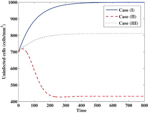
Figure 2. The evolution of latently infected cells.

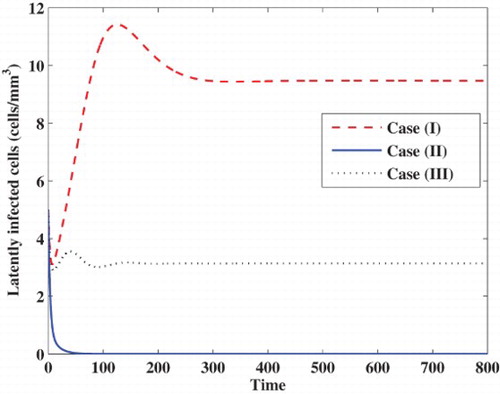
Figure 3. The evolution of actively infected cells.

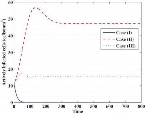
Figure 4. The evolution of free virus particles.

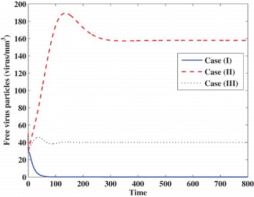
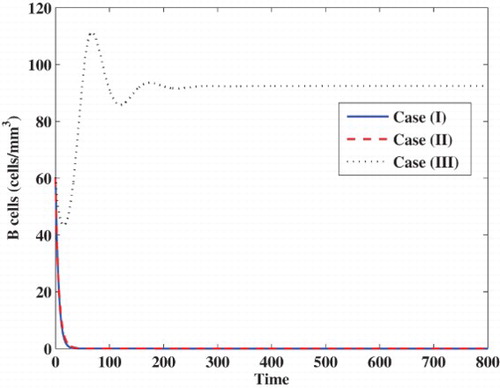
Figure 5. The evolution of B cells.

Case (II) Stability of $E_1$. We take $\beta =0.005$ virus${}^{-1}$ mm${}^3$ day${}^{-1}$ and $g=0.001$ virus${}^{-1}$ mm${}^3$ day${}^{-1}$. In this case, $R_0=1.375>1$ and $R_1=0.882<1$. Figures 1–5 show that the numerical results are consistent with Theorem 2. We can see that, the trajectory of the system will tend to the chronic-infection equilibrium without humoral immune response $E_1(431.67,9.47,47.36,157.87,0)$. In this case, the infection becomes chronic but without persistent humoral immune response.

Case (III) Stability of $E_2$. We choose $\beta =0.005$ virus${}^{-1}$ mm${}^3$ day${}^{-1}$ and $g=0.005$ virus${}^{-1}$ mm${}^3$ day${}^{-1}$. Then we compute $R_0=1.375>1$ and $R_1=1.308>1$. From Figures 1–5 we can see that, our simulation results are consistent with the theoretical results of Theorem 3. We observe that, the trajectory of the system will tend to the chronic-infection equilibrium with humoral immune response $E_2(811.61,3.14,15.7,40,92.49)$. In this case, the infection becomes chronic but with persistent humoral immune response.

4. Conclusion

In this paper, we have proposed and analysed a virus dynamics model with humoral immune response. The model describes the interaction between the uninfected target cells, latently infected cells, actively infected cells, free virus particles and B cells. The incidence rate has been given by Beddington–DeAngelis functional response. We have derived two threshold parameters, the basic infection reproduction number $R_0$ and the humoral immune response activation number $R_1$ which completely determine the basic and global properties of the virus dynamics model. Using Lyapunov method and applying LaSalle's invariance principle we have proven that if $R_0\le 1$, then the infection-free equilibrium is GAS, if $R_1\le 1<R_0$, then the chronic-infection equilibrium without humoral immune response is GAS, and if $R_1>1$, then the chronic-infection equilibrium with humoral immune response is GAS. Numerical simulations have been performed for the model. We have shown that both numerical and theoretical results are consistent.

Acknowledgements

The authors acknowledge with thanks DSR technical and financial support. The authors are also grateful to professor J. M. Cushing and to the anonymous reviewers for constructive suggestions and valuable comments, which improve the quality of the article.

Disclosure statement

No potential conflict of interest was reported by the authors.

Funding

This article was funded by the Deanship of Scientific Research (DSR), King Abdulaziz University, Jeddah.

References

- J.A. Deans and S. Cohen, Immunology of malaria, Ann. Rev. Microbiol. 37 (1983), pp. 25–50. doi: 10.1146/annurev.mi.37.100183.000325
- S. Eikenberry, S. Hews, J.D. Nagy, and Y. Kuang, The dynamics of a delay model of hepatitis B virus infection with logistic hepatocyte growth, Math. Biosc. Eng. 6 (2009), pp. 283–299. doi: 10.3934/mbe.2009.6.283
- A.M. Elaiw, Global properties of a class of HIV models, Nonlinear Anal. Real World Appl. 11 (2010), pp. 2253–2263. doi: 10.1016/j.nonrwa.2009.07.001
- A.M. Elaiw, Global properties of a class of virus infection models with multitarget cells, Nonlinear Dynam. 69 (2012), pp. 423–435. doi: 10.1007/s11071-011-0275-0
- A.M. Elaiw, Global dynamics of an HIV infection model with two classes of target cells and distributed delays, Discrete Dyn. Nat. Soc. 2012. Article ID 253703.
- A.M. Elaiw and S.A. Azoz, Global properties of a class of HIV infection models with Beddington–DeAngelis functional response, Math. Method Appl. Sci. 36 (2013), pp. 383–394. doi: 10.1002/mma.2596
- A.M. Elaiw, I.A. Hassanien, and S.A. Azoz, Global stability of HIV infection models with intracellular delays, J. Korean Math. Soc. 49 (2012), pp. 779–794. doi: 10.4134/JKMS.2012.49.4.779
- J.K. Hale and S.V. Lunel, Introduction to Functional Differential Equations, Springer-Verlag, New York, 1993.
- G. Huang, W. Ma, and Y. Takeuchi, Global properties for virus dynamics model with Beddington–DeAngelis functional response, Appl. Math. Lett. 22 (2009), pp. 1690–1693. doi: 10.1016/j.aml.2009.06.004
- A. Korobeinikov, Global properties of basic virus dynamics models, Bull. Math. Biol. 66 (2004), pp. 879–883. doi: 10.1016/j.bulm.2004.02.001
- M.Y. Li and H. Shu, Global dynamics of a mathematical model for HTLV-I infection of CD4+ T cells with delayed CTL response, Nonlinear Anal. Real World Appl. 13 (2012), pp. 1080–1092. doi: 10.1016/j.nonrwa.2011.02.026
- J. Li, K. Wang, and Y. Yang, Dynamical behaviors of an HBV infection model with logistic hepatocyte growth, Math. Comput. Modelling 54 (2011), pp. 704–711. doi: 10.1016/j.mcm.2011.03.013
- A. Murase, T. Sasaki, and T. Kajiwara, Stability analysis of pathogen-immune interaction dynamics, J. Math. Biol. 51 (2005), pp. 247–267. doi: 10.1007/s00285-005-0321-y
- A.U. Neumann, N.P. Lam, H. Dahari, D.R. Gretch, T.E. Wiley, T.J Layden, and A.S. Perelson, Hepatitis C viral dynamics in vivo and the antiviral efficacy of interferon-alpha therapy, Science 282 (1998), pp. 103–107. doi: 10.1126/science.282.5386.103
- M.A. Nowak and C.R.M. Bangham, Population dynamics of immune responses to persistent viruses, Science 272 (1996), pp. 74–79. doi: 10.1126/science.272.5258.74
- M.A. Nowak and R.M. May, Virus Dynamics: Mathematical Principles of Immunology and Virology, Oxford University, Oxford, 2000.
- M.A. Obaid and A.M. Elaiw, Stability of virus infection models with antibodies and chronically infected cells, Abstr. Appl. Anal. 2014 (2014). Article ID 650371. doi: 10.1155/2014/650371
- A.S. Perelson and P.W. Nelson, Mathematical analysis of HIV-1 dynamics in vivo, SIAM Rev. 41 (1999), pp. 3–44. doi: 10.1137/S0036144598335107
- A.S. Perelson, D.E. Kirschner, and R. De Boer, Dynamics of HIV infection of CD4+ T cells, Math. Biosci. 114(1) (1993), pp. 81–125. doi: 10.1016/0025-5564(93)90043-A
- R. Qesmi, J. Wu, J. Wu, and J.M. Heffernan, Influence of backward bifurcation in a model of hepatitis B and C viruses, Math. Biosci. 224 (2010), pp. 118–125. doi: 10.1016/j.mbs.2010.01.002
- R. Qesmi, S. ElSaadany, J.M. Heffernan, and J. Wu, A hepatitis B and C virus model with age since infection that exhibits backward bifurcation, SIAM J. Appl. Math. 71(4) (2011), pp. 1509–1530. doi: 10.1137/10079690X
- X. Song and A.U. Neumann, Global stability and periodic solution of the viral dynamics, J. Math. Anal. Appl. 329 (2007), pp. 281–297. doi: 10.1016/j.jmaa.2006.06.064
- P. Tanvi, G. Gujarati, and G. Ambika, Virus antibody dynamics in primary and secondary dengue infections, J. Math. Biol. 69 (2014), pp. 1773–1800. doi: 10.1007/s00285-013-0749-4
- L. Wang and M.Y. Li, Mathematical analysis of the global dynamics of a model for HIV infection of CD4+ T cells, Math. Biosci. 200(1) (2006), pp. 44–57. doi: 10.1016/j.mbs.2005.12.026
- S. Wang and D. Zou, Global stability of in-host viral models with humoral immunity and intracellular delays, J. Appl. Math. Model. 36 (2012), pp. 1313–1322. doi: 10.1016/j.apm.2011.07.086