Imitation dynamics of vaccine decision-making behaviours based on the game theory

ABSTRACT

Based on game theory, we propose an age-structured model to investigate the imitation dynamics of vaccine uptake. We first obtain the existence and local stability of equilibria. We show that Hopf bifurcation can occur. We also establish the global stability of the boundary equilibria and persistence of the disease. The theoretical results are supported by numerical simulations.

KEYWORDS:

• SIR model
• game theory
• decision-making
• stability
• Hopf bifurcation

1. Introduction

Infectious diseases are one of the main enemies threatening human's health. Every year millions of people die as a result of various infectious diseases. Mathematical modelling plays a key role in studying and discovering the transmission mechanisms of important diseases. There exists ample theoretical work investigating infectious diseases and very valuable results on the control of epidemic spread have been obtained. In some of the studies [5, 16, 18, 22, 29, 34] on childhood diseases, one eminent feature is that the transmission rates have salient differences since children have different immunities.

Vaccination has been widely considered as one of the effective methods to reducing the morbidity and mortality from infectious diseases. There are two key vaccination policies: voluntary vaccination and mandatory vaccination. There has been a vigorous debate about voluntary vaccination policy failing to protect population adequately. A rational vaccine decision-making is determined by various factors, such as perceived infection risk, potential side effects from vaccination, and vaccinating behaviours of other individuals. Because of the declining familiarity with the interplay between perceived infection risk and potential side effects from vaccination, parents have various reasons for avoiding the potential side effects for their children, relying instead on enough other children being vaccinated to provide herd immunity. Therefore, rational decision may lead to a reduced number of vaccination intakes. This is a free-riding dilemma between individuals and the public good. Game theory builds a bridge connecting the epidemic models with individual behaviours.

Vaccine decision-making based on game theory has been extensively investigated (see, e.g. [1–3, 8, 10–15, 17, 28, 35, 35–38, 40]). In these works, it is usually assumed that individuals have full information for perceived infection risk and potential vaccine health risk. Under this assumption, rational vaccine decision-making will get the highest personal utilities, that is, there exists a Nash equilibrium where no individuals could be better off by unilaterally changing to a different strategy [3, 15]. In [35], Xia and Liu employed a computational approach to characterize the impact of social influence on individuals' vaccination decision-making while in [36] they also investigated the impact of the two factors, information of the disease prevalence and the perceived vaccination risk, and fading coefficient of awareness spread. Recently, Xu and Cresmman [38] built a nonlinear epidemic model with the smoothed best response by game-theory based decisions on vaccination. Their results showed that if there is a perceived cost for vaccination, the smoothed best response is very effective in controlling the disease spread, but if vaccination is free, the best response is a good control. Zhang et al. [40] investigated the ‘double-edged sword’ effect on public health conditions for rational decision-making. Shim et al. used game dynamic models to gain insight into the decision-making between vaccine skeptics and vaccine believers [31] and the decision-making with regard to antiviral intervention during an influenza pandemic [30], respectively.

The above-mentioned references focus on vaccine uptake based on the perfect information the parents mastered on perceived infection risk and potential vaccine side effects. In fact, the vaccine uptake behaviours evolve with respect to time. Individuals' decision on vaccination or not is conducted by imitating others who appear to have adopted more successful strategies. The process is called ‘imitation dynamics’ and it has been studied by some researchers. Bauch [2] investigated parents' vaccinating decisions for their children with the assumption that the susceptibles behave strategically in accordance with imitation dynamics and studied the dependence of epidemic prevalence and coverage of vaccination on these strategic decisions. Fu et al. [17] proposed an agent-based model on social network with game theory to shed light on how imitation of peers shapes individual vaccination choices. d'Onofrio et al. [12] assumed that the perceived risk of vaccination is a function with respect to the incidence and studied an susceptible-infected-removed (SIR) transmission model with dynamic vaccine demand based on an imitation mechanism. A common assumption in these existing vaccination models on imitation dynamics is that individuals are homogeneously mixed or heterogeneously mixed on social networks [9, 11, 37]. This cannot capture the feature of different transmission rates for childhood diseases which we mentioned earlier. In order to address the imitated behaviours on vaccination decision-making, we develop an age-structured epidemic model based on the game theory. We assume that the transmission incidence rate varies according to the infection age and individuals act their behaviours with unperfect information about perceived infection risk and potential vaccine side effects. The payoff of the perceived infection risk is also relative with the infection age. Parents imitate the vaccination decision-making of their neighbours and then adopt a vaccination policy.

The rest of the paper is organized as follows. Based on the game theory, an SIR epidemic model with infection age is introduced in Section 2. We study the existence of equilibria and their local stability in Section 3. A local Hopf bifurcation may occur. Section 4 is devoted to the global stability of boundary equilibria based on the fluctuation lemma and the results for the case without vaccination. We also consider the persistence of disease in Section 4. In Section 5, numerical simulations are provided to demonstrate the theoretical results. The paper concludes with some discussions.

2. The model formulation

In [2], Bauch proposed an epidemic model to predict vaccinating behaviour based on game theory. The total population is divided into three classes: the Susceptible $S\left(t\right)$, the Recovered $R\left(t\right)$, and the Infected $I\left(t\right)$ at time t. It is assumed that all newborns are susceptible; All the groups decrease due to natural death; Susceptible individuals are infected by infectious individuals and enter the infected group; The infectious individuals exit the group due to natural death and recovery; The recovered group increases due to recovered infectious individuals and the vaccinated newborns and decreases due to natural death; The recovered individuals acquire permanent immunity from the disease or vaccination and never leave this group. The incidence has a bilinear form. In order to understand a strategic interaction between individuals when they are deciding whether or not to vaccinate, a replicator equation for an evolution population game is introduced, and the payoff function varies according to time. If x denotes the proportion of children that are vaccinated at birth, the equation for x formally reads as $\frac{\mathrm{d}x}{\mathrm{d}t}=kx(1-x)[-r_v+r_{i}mI],$ where the vaccination cost is $-r_v$ and the non-vaccination cost is $r_{i}mI$. Here $r_i$ denotes the perceived probability of suffering significant morbidity upon infection, m quantifies the sensitivity of vaccinating behaviour to changes in prevalence, k denotes the imitation rate. Under these assumptions, Bauch [2] obtained the following model based on game theory, (1) $\begin{array}{rl}\frac{\mathrm{d}S\left(t\right)}{\mathrm{d}t}& =\mathrm{\Lambda }(1-x)-\beta S\left(t\right)I\left(t\right)-\mu S\left(t\right),\\ \frac{\mathrm{d}I\left(t\right)}{\mathrm{d}t}& =\beta S\left(t\right)I\left(t\right)-(\mu +\gamma )I\left(t\right),\\ \frac{\mathrm{d}R\left(t\right)}{\mathrm{d}t}& =\mathrm{\Lambda }x+\gamma I\left(t\right)-\mu R\left(t\right),\\ \frac{\mathrm{d}x\left(t\right)}{\mathrm{d}t}& =kx(1-x)[-r_v+r_{i}mI],\end{array}$(1) where Λ is the input rate (note that we modified the input rate to be Λ instead of μ as in [2]), β is the transmission rate, μ is the natural death rate, γ is the recovery rate.

It is well-known that most childhood diseases have incubation period (the length of time from when a child is exposed to the illness to when the first symptoms appear in that child). For example, the ranges for the incubation period of measles is 7–21 days [7], of mumps is 16–25 days [26], of pertussis is 4–21 days [27]. During the incubation period, whether the exposed child is infectious or not depends on the disease. During the contagious period (the amount of time during which a sick child can give the disease to others), the infectivity of infectious individuals may vary. Moreover, inadequate vaccination coverage may increase congenital rubella syndrome numbers by increasing the average age at infection[25]. To describe these phenomena, we introduce the infection age. Let $i(t,a)$ denote the density of infected individuals of infection age a at time t. Similar to the bilinear form, we assume that the incidence rate depends on the infectious age a in the following way, $\lambda \left(t\right)=S\left(t\right){\int }_0^{\mathrm{\infty }}\beta \left(a\right)i(t,a)\mathrm{d}a,$ where $\beta \left(a\right)$ is the transmission rate with infection age a. In epidemiology, ${\int }_0^{\mathrm{\infty }}\beta \left(a\right)i(t,a)\mathrm{d}a$ is called the force of infection at time t.

For convenience, the perceived vaccination cost is $-r$; while the potential risk cost for non-vaccinator mainly depends on the epidemic transmission, so its cost is $-{\int }_0^{\mathrm{\infty }}\beta \left(a\right)i(t,a)\mathrm{d}a$, or the payoff benefit is ${\int }_0^{\mathrm{\infty }}\beta \left(a\right)i(t,a)\mathrm{d}a$. Then the payoff gain for a vaccinator compared to a non-vaccinator is ${\int }_0^{\mathrm{\infty }}\beta \left(a\right)i(t,a)\mathrm{d}a-r$. This is formally analogous with [38]. Therefore, similar to [2], we obtain the replicator equation for the portion x of vaccinated children at birth as follows, $\frac{\mathrm{d}x}{\mathrm{d}t}=\delta x(1-x)\left({\int }_0^{\mathrm{\infty }}\beta \left(a\right)i(t,a)\mathrm{d}a-r\right).$ Based on the above assumptions, the model with game theory is given by the following system of ordinary and partial differential equations, (2) $\begin{array}{rl}\frac{\mathrm{d}S\left(t\right)}{\mathrm{d}t}& =\mathrm{\Lambda }(1-x)-S\left(t\right){\int }_0^{\mathrm{\infty }}\beta \left(a\right)i(t,a)\mathrm{d}a-\mu S\left(t\right),\\ \frac{\mathrm{\partial }i(t,a)}{\mathrm{\partial }t}+\frac{\mathrm{\partial }i(t,a)}{\mathrm{\partial }a}& =-(\mu +\gamma (a\left)\right)i(t,a),\\ \frac{\mathrm{d}R\left(t\right)}{\mathrm{d}t}& =\mathrm{\Lambda }x+{\int }_0^{\mathrm{\infty }}\gamma \left(a\right)i(t,a)\mathrm{d}a-\mu R\left(t\right),\\ \frac{\mathrm{d}x\left(t\right)}{\mathrm{d}t}& =\delta x(1-x)\left({\int }_0^{\mathrm{\infty }}\beta \left(a\right)i(t,a)\mathrm{d}a-r\right),\end{array}$(2) with the boundary condition $i(t,0)=S\left(t\right){\int }_0^{\mathrm{\infty }}\beta \left(a\right)i(t,a)\mathrm{d}a,t>0$ and initial conditions $S\left(0\right)=S_0\ge 0,i(0,a)=i_0\left(a\right)\in L_{+}^1,R\left(0\right)=R_0\ge 0,x\left(0\right)=x_0\in [0,1],$ where $L_{+}^1$ is the set of all integrable functions from ${\mathbb{R}}_{+}=[0,\mathrm{\infty })$ into ${\mathbb{R}}_{+}$. $\gamma \left(a\right)$ is the recovered rate with infection age a, δ is the imitation rate which has the familiar biological meaning with k in Equation (1(1) $\begin{array}{rl}\frac{\mathrm{d}S\left(t\right)}{\mathrm{d}t}& =\mathrm{\Lambda }(1-x)-\beta S\left(t\right)I\left(t\right)-\mu S\left(t\right),\\ \frac{\mathrm{d}I\left(t\right)}{\mathrm{d}t}& =\beta S\left(t\right)I\left(t\right)-(\mu +\gamma )I\left(t\right),\\ \frac{\mathrm{d}R\left(t\right)}{\mathrm{d}t}& =\mathrm{\Lambda }x+\gamma I\left(t\right)-\mu R\left(t\right),\\ \frac{\mathrm{d}x\left(t\right)}{\mathrm{d}t}& =kx(1-x)[-r_v+r_{i}mI],\end{array}$(1) ).

Due to the biological background, Λ, μ, δ and r are all positive, and $\beta \ne 0$ belongs to $C_{BU}({\mathbb{R}}_{+},{\mathbb{R}}_{+})$ with β being not identically zero, where $C_{BU}({\mathbb{R}}_{+},{\mathbb{R}}_{+})$ denotes the set of all bounded and uniformly continuous functions from ${\mathbb{R}}_{+}$ into ${\mathbb{R}}_{+}$.

Note that the third equation of (2(2) $\begin{array}{rl}\frac{\mathrm{d}S\left(t\right)}{\mathrm{d}t}& =\mathrm{\Lambda }(1-x)-S\left(t\right){\int }_0^{\mathrm{\infty }}\beta \left(a\right)i(t,a)\mathrm{d}a-\mu S\left(t\right),\\ \frac{\mathrm{\partial }i(t,a)}{\mathrm{\partial }t}+\frac{\mathrm{\partial }i(t,a)}{\mathrm{\partial }a}& =-(\mu +\gamma (a\left)\right)i(t,a),\\ \frac{\mathrm{d}R\left(t\right)}{\mathrm{d}t}& =\mathrm{\Lambda }x+{\int }_0^{\mathrm{\infty }}\gamma \left(a\right)i(t,a)\mathrm{d}a-\mu R\left(t\right),\\ \frac{\mathrm{d}x\left(t\right)}{\mathrm{d}t}& =\delta x(1-x)\left({\int }_0^{\mathrm{\infty }}\beta \left(a\right)i(t,a)\mathrm{d}a-r\right),\end{array}$(2) ) is decoupled from the others. Then we can ignore it and only consider the following system, (3) $\begin{array}{rl}& \frac{\mathrm{d}S\left(t\right)}{\mathrm{d}t}=\mathrm{\Lambda }(1-x)-S\left(t\right){\int }_0^{\mathrm{\infty }}\beta \left(a\right)i(t,a)\mathrm{d}a-\mu S\left(t\right),\\ & \frac{\mathrm{\partial }i(t,a)}{\mathrm{\partial }t}+\frac{\mathrm{\partial }i(t,a)}{\mathrm{\partial }a}=-(\mu +\gamma (a\left)\right)i(t,a),\\ & \frac{\mathrm{d}x\left(t\right)}{\mathrm{d}t}=\delta x(1-x)\left({\int }_0^{\mathrm{\infty }}\beta \left(a\right)i(t,a)\mathrm{d}a-r\right)\end{array}$(3) with the boundary condition $i(t,0)=S\left(t\right){\int }_0^{\mathrm{\infty }}\beta \left(a\right)i(t,a)\mathrm{d}a,t>0$ and initial conditions $S\left(0\right)=S_0\ge 0,i(0,a)=i_0\left(a\right)\in L_{+}^1,x\left(0\right)=x_0\in [0,1].$ Due to Iannelli [21] and Magal [23] , if $i_0$ satisfies the coupling equation $i(0,0)=S_0{\int }_0^{\mathrm{\infty }}\beta \left(a\right)i_0\left(a\right)\mathrm{d}a$ then Equation (3(3) $\begin{array}{rl}& \frac{\mathrm{d}S\left(t\right)}{\mathrm{d}t}=\mathrm{\Lambda }(1-x)-S\left(t\right){\int }_0^{\mathrm{\infty }}\beta \left(a\right)i(t,a)\mathrm{d}a-\mu S\left(t\right),\\ & \frac{\mathrm{\partial }i(t,a)}{\mathrm{\partial }t}+\frac{\mathrm{\partial }i(t,a)}{\mathrm{\partial }a}=-(\mu +\gamma (a\left)\right)i(t,a),\\ & \frac{\mathrm{d}x\left(t\right)}{\mathrm{d}t}=\delta x(1-x)\left({\int }_0^{\mathrm{\infty }}\beta \left(a\right)i(t,a)\mathrm{d}a-r\right)\end{array}$(3) ) is well-posed. In the sequel, whenever we say a solution of Equation (3(3) $\begin{array}{rl}& \frac{\mathrm{d}S\left(t\right)}{\mathrm{d}t}=\mathrm{\Lambda }(1-x)-S\left(t\right){\int }_0^{\mathrm{\infty }}\beta \left(a\right)i(t,a)\mathrm{d}a-\mu S\left(t\right),\\ & \frac{\mathrm{\partial }i(t,a)}{\mathrm{\partial }t}+\frac{\mathrm{\partial }i(t,a)}{\mathrm{\partial }a}=-(\mu +\gamma (a\left)\right)i(t,a),\\ & \frac{\mathrm{d}x\left(t\right)}{\mathrm{d}t}=\delta x(1-x)\left({\int }_0^{\mathrm{\infty }}\beta \left(a\right)i(t,a)\mathrm{d}a-r\right)\end{array}$(3) ), the above assumptions on the boundary and initial conditions are satisfied.

Proposition 2.1.

Let $\left(S\right(t),i(t,a),x(t\left)\right)$ be a solution of Equation (3(3) $\begin{array}{rl}& \frac{\mathrm{d}S\left(t\right)}{\mathrm{d}t}=\mathrm{\Lambda }(1-x)-S\left(t\right){\int }_0^{\mathrm{\infty }}\beta \left(a\right)i(t,a)\mathrm{d}a-\mu S\left(t\right),\\ & \frac{\mathrm{\partial }i(t,a)}{\mathrm{\partial }t}+\frac{\mathrm{\partial }i(t,a)}{\mathrm{\partial }a}=-(\mu +\gamma (a\left)\right)i(t,a),\\ & \frac{\mathrm{d}x\left(t\right)}{\mathrm{d}t}=\delta x(1-x)\left({\int }_0^{\mathrm{\infty }}\beta \left(a\right)i(t,a)\mathrm{d}a-r\right)\end{array}$(3) ) with the maximal interval of existence $[0,\rho )$ ($\rho$ is allowed to be $\mathrm{\infty }$) . Then $S\left(t\right)\ge 0,$ $i(t,a)\ge 0,$ and $x\left(t\right)\in [0,1]$ for $t\in [0,\rho )$ and $a\in {\mathbb{R}}_{+}$.

Proof.

Firstly, from the third equation of (3(3) $\begin{array}{rl}& \frac{\mathrm{d}S\left(t\right)}{\mathrm{d}t}=\mathrm{\Lambda }(1-x)-S\left(t\right){\int }_0^{\mathrm{\infty }}\beta \left(a\right)i(t,a)\mathrm{d}a-\mu S\left(t\right),\\ & \frac{\mathrm{\partial }i(t,a)}{\mathrm{\partial }t}+\frac{\mathrm{\partial }i(t,a)}{\mathrm{\partial }a}=-(\mu +\gamma (a\left)\right)i(t,a),\\ & \frac{\mathrm{d}x\left(t\right)}{\mathrm{d}t}=\delta x(1-x)\left({\int }_0^{\mathrm{\infty }}\beta \left(a\right)i(t,a)\mathrm{d}a-r\right)\end{array}$(3) ), we have (4) $x\left(t\right)=\frac{x_0{\mathrm{e}}^{\delta {\int }_0^t\left({\int }_0^{\mathrm{\infty }}\beta \left(a\right)i(s,a)\mathrm{d}a-r\right)\mathrm{d}s}}{1-x_0+x_0{\mathrm{e}}^{\delta {\int }_0^t\left({\int }_0^{\mathrm{\infty }}\beta \right(a\left)i\right(s,a)\mathrm{d}a-r)\mathrm{d}s}}\text{for}t\in [0,\rho ).$(4) Since $x_0\in [0,1]$, it follows that $x\left(t\right)\in [0,1]$ for $t\in [0,\rho )$.

Secondly, by the first equation of (3(3) $\begin{array}{rl}& \frac{\mathrm{d}S\left(t\right)}{\mathrm{d}t}=\mathrm{\Lambda }(1-x)-S\left(t\right){\int }_0^{\mathrm{\infty }}\beta \left(a\right)i(t,a)\mathrm{d}a-\mu S\left(t\right),\\ & \frac{\mathrm{\partial }i(t,a)}{\mathrm{\partial }t}+\frac{\mathrm{\partial }i(t,a)}{\mathrm{\partial }a}=-(\mu +\gamma (a\left)\right)i(t,a),\\ & \frac{\mathrm{d}x\left(t\right)}{\mathrm{d}t}=\delta x(1-x)\left({\int }_0^{\mathrm{\infty }}\beta \left(a\right)i(t,a)\mathrm{d}a-r\right)\end{array}$(3) ), we see that $S\left(t\right)=S_0{\mathrm{e}}^{-\mu t-{\int }_0^t{\int }_0^{\mathrm{\infty }}\beta \left(a\right)i(s,a)\mathrm{d}ads}+\mathrm{\Lambda }{\int }_0^t(1-x(s\left)\right){\mathrm{e}}^{-\mu (t-u)-{\int }_u^t{\int }_0^{\mathrm{\infty }}\beta \left(a\right)i(s,a)\mathrm{d}a\mathrm{d}s}\mathrm{d}u$ for $t\in [0,\rho )$. Clearly, $S\left(t\right)\ge 0$ for $t\in [0,\rho )$ as $S_0\ge 0$ and $x\left(t\right)\in [0,1]$ for $t\in [0,\rho )$.

Now, for any $\xi \in [0,\rho )$, we claim that $i(t,a)\ge 0$ for $t\in [0,\xi ]$ and $a\in {\mathbb{R}}_{+}$ (the idea of the proof is borrowed from Browne and Plyugin [6]). By way of contradiction, assume that there exists $t_0\in [0,\xi ]$ and $a_0\in {\mathbb{R}}_{+}$ such that $i(t_0,a_0)<0$. Integrating the second equation of (3(3) $\begin{array}{rl}& \frac{\mathrm{d}S\left(t\right)}{\mathrm{d}t}=\mathrm{\Lambda }(1-x)-S\left(t\right){\int }_0^{\mathrm{\infty }}\beta \left(a\right)i(t,a)\mathrm{d}a-\mu S\left(t\right),\\ & \frac{\mathrm{\partial }i(t,a)}{\mathrm{\partial }t}+\frac{\mathrm{\partial }i(t,a)}{\mathrm{\partial }a}=-(\mu +\gamma (a\left)\right)i(t,a),\\ & \frac{\mathrm{d}x\left(t\right)}{\mathrm{d}t}=\delta x(1-x)\left({\int }_0^{\mathrm{\infty }}\beta \left(a\right)i(t,a)\mathrm{d}a-r\right)\end{array}$(3) ) with the boundary condition yields that, for $t\in [0,\xi ]$ and $a\in {\mathbb{R}}_{+}$, we have (5) $i(t,a)=\left\{\begin{array}{ll}B(t-a)\pi \left(a\right),& t\ge a,\\ i_0(a-t)\frac{\pi \left(a\right)}{\pi (a-t)},& t<a,\end{array}\right.$(5) where $B\left(t\right)=i(t,0)=S\left(t\right){\int }_0^{\mathrm{\infty }}\beta \left(a\right)i(t,a)\mathrm{d}a$ for $t\in [0,\xi ]$ and $\pi \left(a\right)={\mathrm{e}}^{-{\int }_0^a(\mu +\gamma (s\left)\right)\mathrm{d}s}$ for $a\in {\mathbb{R}}_{+}$. Since $i_0\in L_{+}^1$, we have $a_0<t_0$ and $B(t_0-a_0)<0$. Let $t_{\ast }=inf\{t\in [0,\xi ]:B(t)<0\}$. Then $t_{\ast }\in [0,\xi )$. By the continuity of $B\left(t\right)$ and the definition of $t_{\ast }$, we know that $B\left(t\right)\ge 0$ for $t\in [0,t_{\ast })$ and $B\left(t_{\ast }\right)=0$. Note that, with the help of Equation (5(5) $i(t,a)=\left\{\begin{array}{ll}B(t-a)\pi \left(a\right),& t\ge a,\\ i_0(a-t)\frac{\pi \left(a\right)}{\pi (a-t)},& t<a,\end{array}\right.$(5) ), $\begin{array}{rl}B\left(t\right)& =S\left(t\right){\int }_0^t\beta \left(a\right)B(t-a)\pi \left(a\right)\mathrm{d}a+S\left(t\right){\int }_t^{\mathrm{\infty }}\beta \left(a\right)i_0(a-t)\frac{\pi \left(a\right)}{\pi (a-t)}\mathrm{d}a\\ & =S\left(t\right){\int }_0^t\beta (t-a)B\left(a\right)\pi (t-a)\mathrm{d}a+S\left(t\right){\int }_t^{\mathrm{\infty }}\beta \left(a\right)i_0(a-t)\frac{\pi \left(a\right)}{\pi (a-t)}\mathrm{d}a\end{array}$ for $t\in [0,\xi ]$. Since B is continuous on $[0,\xi ]$ and $B\left(t_{\ast }\right)=0$, there exists an ${\epsilon }_1\in (0,\xi -t_{\ast })$ such that $-\frac{1}{2}\le B\left(t\right)\le \frac{1}{2}$ for $t\in [t_{\ast },t_{\ast }+{\epsilon }_1]$. Let $\hat{S}=max\left\{S\right(t):t\in [0,\xi \left]\right\}$ and $\overline{\beta }=sup\left\{\beta \right(a):a\in {\mathbb{R}}_{+}\}(>0)$. Denote $\epsilon =min\{{\epsilon }_1,\frac{1}{3\overline{\beta }(\hat{S}+1)}\}$. Let $Y=C\left(\right[0,t_{\ast }+\epsilon ],{\mathbb{R}}_{+})$ and $S=\{\varphi \in Y:\varphi (t)=B(t)\mathrm{for}t\in [0,t_{\ast }\left]\mathrm{and}\varphi \right(t)\in [0,1]\mathrm{for}t\in [t_{\ast },t_{\ast }+\epsilon \left]\right\}$. Then Y is a complete distance space with the supremum distance and S is a closed subset of Y . Define L on S by $\left(L\varphi \right)\left(t\right)=S\left(t\right){\int }_0^t\beta (t-a)\varphi \left(a\right)\pi \left(a\right)\mathrm{d}a+S\left(t\right){\int }_t^{\mathrm{\infty }}\beta \left(a\right)i_0(a-t)\frac{\pi \left(a\right)}{\pi (a-t)}\mathrm{d}a.$ Obviously, $L\left(S\right)\subset Y$. Note that $L\varphi {|}_{[0,t_{\ast }]}=B{|}_{[0,t_{\ast }]}$ for $\varphi \in S$ and $LB=B$. Then, for $\varphi \in S$ and $t\in [t_{\ast },t_{\ast }+\epsilon ]$, we have $\begin{array}{rl}0& \le \left(L\varphi \right)\left(t\right)=\left[\right(L\varphi \left)\right(t)-(LB\left)\right(t\left)\right]+\left(LB\right)\left(t\right)\\ & =\left[\right(L\varphi \left)\right(t)-(LB\left)\right(t\left)\right]+B\left(t\right)\\ & =S\left(t\right){\int }_{t_{\ast }}^t\beta (t-a)\left(\varphi \right(a)-B(a\left)\right)\pi (t-a)\mathrm{d}a+B\left(t\right)\\ & \le \frac{3}{2}\hat{S}\overline{\beta }\epsilon +\frac{1}{2}\\ & \le 1\end{array}$ and this shows that L is a mapping from S into itself. Moreover, for ${\varphi }_1$, $\varphi \in S$, we have $\begin{array}{rl}\parallel L{\varphi }_1-L{\varphi }_2\parallel & =max\left\{|\right(L{\varphi }_1\left)\right(t)-(L{\varphi }_2\left)\right(t)|:t\in [t_{\ast },t_{\ast }+\epsilon \left]\right\}\\ & =max\left\{|S\right(t\left){\int }_{t_{\ast }}^t\beta \right(t-a\left)\right({\varphi }_1\left(a\right)-{\varphi }_2\left(a\right)\left)\pi \right(a)\mathrm{d}a|:t\in [t_{\ast },t_{\ast }+\epsilon \left]\right\}\\ & \le \hat{S}\overline{\beta }\epsilon \parallel {\varphi }_1-{\varphi }_2\parallel \\ & <\frac{1}{3}\parallel {\varphi }_1-{\varphi }_2\parallel ,\end{array}$ that is, L is a contraction mapping on S. By the Banach Fixed Point Theorem, there exists a unique $\hat{\varphi }\in S$ such that $\hat{\varphi }\left(t\right)=S\left(t\right){\int }_0^t\beta (t-a)\hat{\varphi }\left(a\right)\pi (t-a)\mathrm{d}a+S\left(t\right){\int }_t^{\mathrm{\infty }}\beta \left(a\right)i_0(a-t)\frac{\pi \left(a\right)}{\pi (a-t)}\mathrm{d}a$ for $t\in [0,t_{\ast }+\epsilon ]$. By the uniqueness of solutions, we have $B\left(t\right)=\hat{\varphi }\left(t\right)$ for $t\in [0,t_{\ast }+\epsilon ]$. This contradicts the definition of $t_{\ast }$ and hence we have proved the claim. Since ξ is arbitrary, we see that $i(t,a)\ge 0$ for $t\in [0,\rho )$ and $a\in {\mathbb{R}}_{+}$. This completes the proof.

Proposition 2.1 implies that $i(t,\cdot )\in L_{+}^1$ for $t\in [0,\rho )$. Setting $N\left(t\right)=S\left(t\right)+{\int }_0^{\mathrm{\infty }}i(t,a)\mathrm{d}a$ for $t\in [0,\rho )$. With the help of Proposition 2.1, we can obtain (6) $\frac{\mathrm{d}N\left(t\right)}{\mathrm{d}t}\le \mathrm{\Lambda }-\mu N\left(t\right)$(6) for $t\in [0,\rho )$, which implies that $\underset{t\to {\rho }^{-}}{lim sup}N\left(t\right)<\mathrm{\infty }$. Therefore, the maximal interval of existence for every solution of Equation (3(3) $\begin{array}{rl}& \frac{\mathrm{d}S\left(t\right)}{\mathrm{d}t}=\mathrm{\Lambda }(1-x)-S\left(t\right){\int }_0^{\mathrm{\infty }}\beta \left(a\right)i(t,a)\mathrm{d}a-\mu S\left(t\right),\\ & \frac{\mathrm{\partial }i(t,a)}{\mathrm{\partial }t}+\frac{\mathrm{\partial }i(t,a)}{\mathrm{\partial }a}=-(\mu +\gamma (a\left)\right)i(t,a),\\ & \frac{\mathrm{d}x\left(t\right)}{\mathrm{d}t}=\delta x(1-x)\left({\int }_0^{\mathrm{\infty }}\beta \left(a\right)i(t,a)\mathrm{d}a-r\right)\end{array}$(3) ) is ${\mathbb{R}}_{+}$. Let $\mathrm{\Phi }:{\mathbb{R}}_{+}\times ({\mathbb{R}}_{+}\times L_{+}^1\times [0,1\left]\right)\to {\mathbb{R}}_{+}\times L_{+}^1\times [0,1]$ be the solution semiflow associated with Equation (3(3) $\begin{array}{rl}& \frac{\mathrm{d}S\left(t\right)}{\mathrm{d}t}=\mathrm{\Lambda }(1-x)-S\left(t\right){\int }_0^{\mathrm{\infty }}\beta \left(a\right)i(t,a)\mathrm{d}a-\mu S\left(t\right),\\ & \frac{\mathrm{\partial }i(t,a)}{\mathrm{\partial }t}+\frac{\mathrm{\partial }i(t,a)}{\mathrm{\partial }a}=-(\mu +\gamma (a\left)\right)i(t,a),\\ & \frac{\mathrm{d}x\left(t\right)}{\mathrm{d}t}=\delta x(1-x)\left({\int }_0^{\mathrm{\infty }}\beta \left(a\right)i(t,a)\mathrm{d}a-r\right)\end{array}$(3) ), that is, $\mathrm{\Phi }(t,(S_0,i_0,x_0\left)\right)=\left(S\right(t),i(t,\cdot ),x(t\left)\right)\text{for}(S_0,i_0,x_0)\in {\mathbb{R}}_{+}\times L_{+}^1\times [0,1].$

Note that, by Equation (6(6) $\frac{\mathrm{d}N\left(t\right)}{\mathrm{d}t}\le \mathrm{\Lambda }-\mu N\left(t\right)$(6) ), $\underset{t\to \mathrm{\infty }}{lim sup}N\left(t\right)\le \mathrm{\Lambda }/\mu$. Moreover, if $N\left(t_0\right)\le \mathrm{\Lambda }/\mu$ for some $t_0\in {\mathbb{R}}_{+}$ then $N\left(t\right)\le \mathrm{\Lambda }/\mu$ for all $t\ge t_0$. Define $\mathrm{\Gamma }=\left\{(S,i,x)\in {\mathbb{R}}_{+}\times L_{+}^1\times [0,1]:S+{\int }_0^{\mathrm{\infty }}i\left(a\right)\mathrm{d}a\le \frac{\mathrm{\Lambda }}{\mu }\right\}.$ Then we have proved the following result.

Proposition 2.2.

Γ is an attractive and positively invariant set for Equation (3(3) $\begin{array}{rl}& \frac{\mathrm{d}S\left(t\right)}{\mathrm{d}t}=\mathrm{\Lambda }(1-x)-S\left(t\right){\int }_0^{\mathrm{\infty }}\beta \left(a\right)i(t,a)\mathrm{d}a-\mu S\left(t\right),\\ & \frac{\mathrm{\partial }i(t,a)}{\mathrm{\partial }t}+\frac{\mathrm{\partial }i(t,a)}{\mathrm{\partial }a}=-(\mu +\gamma (a\left)\right)i(t,a),\\ & \frac{\mathrm{d}x\left(t\right)}{\mathrm{d}t}=\delta x(1-x)\left({\int }_0^{\mathrm{\infty }}\beta \left(a\right)i(t,a)\mathrm{d}a-r\right)\end{array}$(3) ).

To end this section, we mention that, by Equation (4(4) $x\left(t\right)=\frac{x_0{\mathrm{e}}^{\delta {\int }_0^t\left({\int }_0^{\mathrm{\infty }}\beta \left(a\right)i(s,a)\mathrm{d}a-r\right)\mathrm{d}s}}{1-x_0+x_0{\mathrm{e}}^{\delta {\int }_0^t\left({\int }_0^{\mathrm{\infty }}\beta \right(a\left)i\right(s,a)\mathrm{d}a-r)\mathrm{d}s}}\text{for}t\in [0,\rho ).$(4) ), both sets $\left\{\right(S,i,x)\in \mathrm{\Gamma }:x=0\}$ and $\left\{\right(S,i,x)\in \mathrm{\Gamma }:x=1\}$ are also positively invariant subsets of Equation (3(3) $\begin{array}{rl}& \frac{\mathrm{d}S\left(t\right)}{\mathrm{d}t}=\mathrm{\Lambda }(1-x)-S\left(t\right){\int }_0^{\mathrm{\infty }}\beta \left(a\right)i(t,a)\mathrm{d}a-\mu S\left(t\right),\\ & \frac{\mathrm{\partial }i(t,a)}{\mathrm{\partial }t}+\frac{\mathrm{\partial }i(t,a)}{\mathrm{\partial }a}=-(\mu +\gamma (a\left)\right)i(t,a),\\ & \frac{\mathrm{d}x\left(t\right)}{\mathrm{d}t}=\delta x(1-x)\left({\int }_0^{\mathrm{\infty }}\beta \left(a\right)i(t,a)\mathrm{d}a-r\right)\end{array}$(3) ). It is clear that for solutions in $\left\{\right(S,i,x)\in \mathrm{\Gamma }:x=1\}$ we have $\underset{t\to \mathrm{\infty }}{lim}\left(S\right(t),i(t,a),x(t\left)\right)=(0,0,1)$ for $a\in {\mathbb{R}}_{+}$. On the other invariant set $\left\{\right(S,i,x)\in \mathrm{\Gamma }:x=0\}$, Equation (3(3) $\begin{array}{rl}& \frac{\mathrm{d}S\left(t\right)}{\mathrm{d}t}=\mathrm{\Lambda }(1-x)-S\left(t\right){\int }_0^{\mathrm{\infty }}\beta \left(a\right)i(t,a)\mathrm{d}a-\mu S\left(t\right),\\ & \frac{\mathrm{\partial }i(t,a)}{\mathrm{\partial }t}+\frac{\mathrm{\partial }i(t,a)}{\mathrm{\partial }a}=-(\mu +\gamma (a\left)\right)i(t,a),\\ & \frac{\mathrm{d}x\left(t\right)}{\mathrm{d}t}=\delta x(1-x)\left({\int }_0^{\mathrm{\infty }}\beta \left(a\right)i(t,a)\mathrm{d}a-r\right)\end{array}$(3) ) reduces to the case without vaccination, that is, (7) $\begin{array}{rl}& \frac{\mathrm{d}S\left(t\right)}{\mathrm{d}t}=\mathrm{\Lambda }-S\left(t\right){\int }_0^{\mathrm{\infty }}\beta \left(a\right)i(t,a)\mathrm{d}a-\mu S\left(t\right),\\ & \frac{\mathrm{\partial }i(t,a)}{\mathrm{\partial }t}+\frac{\mathrm{\partial }i(t,a)}{\mathrm{\partial }a}=-(\mu +\gamma (a\left)\right)i(t,a).\end{array}$(7) This model has been studied by Magal et al. [24] and their main results are as follows.

Theorem 2.3

[24, Theorems 1.2 and 1.3]

1. If $\mathrm{\Lambda }{\int }_0^{\mathrm{\infty }}\beta \left(a\right)\pi \left(a\right)\mathrm{d}a/\mu \le 1$ then the disease free equilibrium $(\mathrm{\Lambda }/\mu ,0)$ is globally asymptotically stable for the semiflow generated by Equation (7(7) $\begin{array}{rl}& \frac{\mathrm{d}S\left(t\right)}{\mathrm{d}t}=\mathrm{\Lambda }-S\left(t\right){\int }_0^{\mathrm{\infty }}\beta \left(a\right)i(t,a)\mathrm{d}a-\mu S\left(t\right),\\ & \frac{\mathrm{\partial }i(t,a)}{\mathrm{\partial }t}+\frac{\mathrm{\partial }i(t,a)}{\mathrm{\partial }a}=-(\mu +\gamma (a\left)\right)i(t,a).\end{array}$(7) ).

2. Let $\overline{a}=sup\{a\ge 0:\beta (a)>0\}$ and $M_0={\mathbb{R}}_{+}\times \{i\in L_{+}^1:{\int }_0^{\overline{a}}i(a)\mathrm{d}a>0\}\mathrm{and}\mathrm{\partial }{M}_0=({\mathbb{R}}_{+}\times L_{+}^1)\setminus M_0.$ Assume $\mathrm{\Lambda }{\int }_0^{\mathrm{\infty }}\beta \left(a\right)\pi \left(a\right)\mathrm{d}a/\mu >1$. Then every solution of Equation (7(7) $\begin{array}{rl}& \frac{\mathrm{d}S\left(t\right)}{\mathrm{d}t}=\mathrm{\Lambda }-S\left(t\right){\int }_0^{\mathrm{\infty }}\beta \left(a\right)i(t,a)\mathrm{d}a-\mu S\left(t\right),\\ & \frac{\mathrm{\partial }i(t,a)}{\mathrm{\partial }t}+\frac{\mathrm{\partial }i(t,a)}{\mathrm{\partial }a}=-(\mu +\gamma (a\left)\right)i(t,a).\end{array}$(7) ) with the initial value in $\mathrm{\partial }{M}_0$ $($respectively, in $M_0)$ stays in $\mathrm{\partial }{M}_0$ $($respectively, in $M_0)$. Moreover, each solution with initial value in $\mathrm{\partial }{M}_0$ converges to $(\mathrm{\Lambda }/\mu ,0)$. Furthermore, every solution with an initial value in $M_0$ converges to the endemic equilibrium $(1/{\int }_0^{\mathrm{\infty }}\beta \left(a\right)\pi \left(a\right)\mathrm{d}a,(\mathrm{\Lambda }-\mu /{\int }_0^{\mathrm{\infty }}\beta \left(a\right)\pi \left(a\right)\mathrm{d}a\left)\pi \right(a\left)\right)$, which is locally asymptotically stable.

The attractivity of the endemic equilibrium in Theorem 2.3(ii) is established by the approach of Lyapunov functionals. We also mention that Theorem 2.3 will play an important role in dealing with the attractivity of the boundary equilibria of Equation (3(3) $\begin{array}{rl}& \frac{\mathrm{d}S\left(t\right)}{\mathrm{d}t}=\mathrm{\Lambda }(1-x)-S\left(t\right){\int }_0^{\mathrm{\infty }}\beta \left(a\right)i(t,a)\mathrm{d}a-\mu S\left(t\right),\\ & \frac{\mathrm{\partial }i(t,a)}{\mathrm{\partial }t}+\frac{\mathrm{\partial }i(t,a)}{\mathrm{\partial }a}=-(\mu +\gamma (a\left)\right)i(t,a),\\ & \frac{\mathrm{d}x\left(t\right)}{\mathrm{d}t}=\delta x(1-x)\left({\int }_0^{\mathrm{\infty }}\beta \left(a\right)i(t,a)\mathrm{d}a-r\right)\end{array}$(3) ).

3. Existence of equilibria and their local stability

Recall that $\pi \left(a\right)={\mathrm{e}}^{-{\int }_0^a(\mu +\gamma (s\left)\right)\mathrm{d}s}$ for $a\in {\mathbb{R}}_{+}$. Define $K={\int }_0^{\mathrm{\infty }}\beta \left(a\right)\pi \left(a\right)\mathrm{d}a$ and ${\mathcal{R}}_0=\frac{\mathrm{\Lambda }K}{\mu }.$ Note that $\pi \left(a\right)$ is the survival probability at infection age a and hence K is the mean value of the infectivity of an exposed child. As the total population size is $\mathrm{\Lambda }/\mu$, ${\mathcal{R}}_0$ is the average number of cases that one typical infected individual can produce during the infectious period. In epidemiology, ${\mathcal{R}}_0$ is called the basic reproduction umber. As we will see soon, the structure of equilibria of Equation (3(3) $\begin{array}{rl}& \frac{\mathrm{d}S\left(t\right)}{\mathrm{d}t}=\mathrm{\Lambda }(1-x)-S\left(t\right){\int }_0^{\mathrm{\infty }}\beta \left(a\right)i(t,a)\mathrm{d}a-\mu S\left(t\right),\\ & \frac{\mathrm{\partial }i(t,a)}{\mathrm{\partial }t}+\frac{\mathrm{\partial }i(t,a)}{\mathrm{\partial }a}=-(\mu +\gamma (a\left)\right)i(t,a),\\ & \frac{\mathrm{d}x\left(t\right)}{\mathrm{d}t}=\delta x(1-x)\left({\int }_0^{\mathrm{\infty }}\beta \left(a\right)i(t,a)\mathrm{d}a-r\right)\end{array}$(3) ) depends on the values of ${\mathcal{R}}_0$. $(S^{\ast },i^{\ast },x^{\ast })\in {\mathbb{R}}_{+}\times L_{+}^1\times [0,1]$

is an equilibrium of Equation (3(3) $\begin{array}{rl}& \frac{\mathrm{d}S\left(t\right)}{\mathrm{d}t}=\mathrm{\Lambda }(1-x)-S\left(t\right){\int }_0^{\mathrm{\infty }}\beta \left(a\right)i(t,a)\mathrm{d}a-\mu S\left(t\right),\\ & \frac{\mathrm{\partial }i(t,a)}{\mathrm{\partial }t}+\frac{\mathrm{\partial }i(t,a)}{\mathrm{\partial }a}=-(\mu +\gamma (a\left)\right)i(t,a),\\ & \frac{\mathrm{d}x\left(t\right)}{\mathrm{d}t}=\delta x(1-x)\left({\int }_0^{\mathrm{\infty }}\beta \left(a\right)i(t,a)\mathrm{d}a-r\right)\end{array}$(3) ) if it satisfies (8) $\begin{array}{rl}0& =\mathrm{\Lambda }(1-x^{\ast })-S^{\ast }{\int }_0^{\mathrm{\infty }}\beta \left(a\right)i^{\ast }\left(a\right)\mathrm{d}a-\mu S^{\ast },\\ \frac{\mathrm{d}{i}^{\ast }\left(a\right)}{\mathrm{d}a}& =-(\mu +\gamma (a\left)\right)i^{\ast }\left(a\right),\\ i^{\ast }\left(0\right)& =S^{\ast }{\int }_0^{\mathrm{\infty }}\beta \left(a\right)i^{\ast }\left(a\right)\mathrm{d}a,\\ 0& =\delta x^{\ast }(1-x^{\ast })\left({\int }_0^{\mathrm{\infty }}\beta \right(a\left)i^{\ast }\right(a)\mathrm{d}a-r).\end{array}$(8) By direct computation, we easily see that Equation (8(8) $\begin{array}{rl}0& =\mathrm{\Lambda }(1-x^{\ast })-S^{\ast }{\int }_0^{\mathrm{\infty }}\beta \left(a\right)i^{\ast }\left(a\right)\mathrm{d}a-\mu S^{\ast },\\ \frac{\mathrm{d}{i}^{\ast }\left(a\right)}{\mathrm{d}a}& =-(\mu +\gamma (a\left)\right)i^{\ast }\left(a\right),\\ i^{\ast }\left(0\right)& =S^{\ast }{\int }_0^{\mathrm{\infty }}\beta \left(a\right)i^{\ast }\left(a\right)\mathrm{d}a,\\ 0& =\delta x^{\ast }(1-x^{\ast })\left({\int }_0^{\mathrm{\infty }}\beta \right(a\left)i^{\ast }\right(a)\mathrm{d}a-r).\end{array}$(8) ) can have at most four equilibria, $E_1=(0,0,1)$, $E_2=(\mathrm{\Lambda }/\mu ,0,0)$, $E_3=(S^{\ast },i_1^{\ast }(0\left)\pi \right(a),0)$, $E_4=(S^{\ast },i^{\ast }(0\left)\pi \right(a),x^{\ast })$, where $S^{\ast }=\frac{1}{K},i_1^{\ast }\left(0\right)=\frac{\mu }{K}({\mathcal{R}}_0-1),i^{\ast }\left(0\right)=\frac{r}{K},x^{\ast }=\frac{\mu ({\mathcal{R}}_0-1)-r}{\mathrm{\Lambda }K}.$ The existence of equilibria of Equation (3(3) $\begin{array}{rl}& \frac{\mathrm{d}S\left(t\right)}{\mathrm{d}t}=\mathrm{\Lambda }(1-x)-S\left(t\right){\int }_0^{\mathrm{\infty }}\beta \left(a\right)i(t,a)\mathrm{d}a-\mu S\left(t\right),\\ & \frac{\mathrm{\partial }i(t,a)}{\mathrm{\partial }t}+\frac{\mathrm{\partial }i(t,a)}{\mathrm{\partial }a}=-(\mu +\gamma (a\left)\right)i(t,a),\\ & \frac{\mathrm{d}x\left(t\right)}{\mathrm{d}t}=\delta x(1-x)\left({\int }_0^{\mathrm{\infty }}\beta \left(a\right)i(t,a)\mathrm{d}a-r\right)\end{array}$(3) ) is summarized below.

Theorem 3.1.

1. If ${\mathcal{R}}_0\le 1$ then Equation (3(3) $\begin{array}{rl}& \frac{\mathrm{d}S\left(t\right)}{\mathrm{d}t}=\mathrm{\Lambda }(1-x)-S\left(t\right){\int }_0^{\mathrm{\infty }}\beta \left(a\right)i(t,a)\mathrm{d}a-\mu S\left(t\right),\\ & \frac{\mathrm{\partial }i(t,a)}{\mathrm{\partial }t}+\frac{\mathrm{\partial }i(t,a)}{\mathrm{\partial }a}=-(\mu +\gamma (a\left)\right)i(t,a),\\ & \frac{\mathrm{d}x\left(t\right)}{\mathrm{d}t}=\delta x(1-x)\left({\int }_0^{\mathrm{\infty }}\beta \left(a\right)i(t,a)\mathrm{d}a-r\right)\end{array}$(3) ) has two equilibria $E_1$ and $E_2$.

2. If $1<{\mathcal{R}}_0\le 1+r/\mu$ then Equation (3(3) $\begin{array}{rl}& \frac{\mathrm{d}S\left(t\right)}{\mathrm{d}t}=\mathrm{\Lambda }(1-x)-S\left(t\right){\int }_0^{\mathrm{\infty }}\beta \left(a\right)i(t,a)\mathrm{d}a-\mu S\left(t\right),\\ & \frac{\mathrm{\partial }i(t,a)}{\mathrm{\partial }t}+\frac{\mathrm{\partial }i(t,a)}{\mathrm{\partial }a}=-(\mu +\gamma (a\left)\right)i(t,a),\\ & \frac{\mathrm{d}x\left(t\right)}{\mathrm{d}t}=\delta x(1-x)\left({\int }_0^{\mathrm{\infty }}\beta \left(a\right)i(t,a)\mathrm{d}a-r\right)\end{array}$(3) ) has three equilibria $E_1,$ $E_2,$ and $E_3$.

3. If ${\mathcal{R}}_0>1+r/\mu$ then Equation (3(3) $\begin{array}{rl}& \frac{\mathrm{d}S\left(t\right)}{\mathrm{d}t}=\mathrm{\Lambda }(1-x)-S\left(t\right){\int }_0^{\mathrm{\infty }}\beta \left(a\right)i(t,a)\mathrm{d}a-\mu S\left(t\right),\\ & \frac{\mathrm{\partial }i(t,a)}{\mathrm{\partial }t}+\frac{\mathrm{\partial }i(t,a)}{\mathrm{\partial }a}=-(\mu +\gamma (a\left)\right)i(t,a),\\ & \frac{\mathrm{d}x\left(t\right)}{\mathrm{d}t}=\delta x(1-x)\left({\int }_0^{\mathrm{\infty }}\beta \left(a\right)i(t,a)\mathrm{d}a-r\right)\end{array}$(3) ) has four equilibria $E_1,$ $E_2,$ $E_3,$ and $E_4$.

From the biological viewpoint, $E_1$ is the disease free and pure vaccinator strategy equilibrium, $E_2$ is the disease free and non-vaccinator strategy equilibrium, $E_3$ is the endemic and non-vaccinator strategy equilibrium, and $E_4$ is the endemic and vaccinator strategy equilibrium.

Let ${\overline{E}}^{\ast }=({\overline{S}}^{\ast },{\overline{i}}^{\ast },{\overline{x}}^{\ast })$ be an equilibrium of Equation (3(3) $\begin{array}{rl}& \frac{\mathrm{d}S\left(t\right)}{\mathrm{d}t}=\mathrm{\Lambda }(1-x)-S\left(t\right){\int }_0^{\mathrm{\infty }}\beta \left(a\right)i(t,a)\mathrm{d}a-\mu S\left(t\right),\\ & \frac{\mathrm{\partial }i(t,a)}{\mathrm{\partial }t}+\frac{\mathrm{\partial }i(t,a)}{\mathrm{\partial }a}=-(\mu +\gamma (a\left)\right)i(t,a),\\ & \frac{\mathrm{d}x\left(t\right)}{\mathrm{d}t}=\delta x(1-x)\left({\int }_0^{\mathrm{\infty }}\beta \left(a\right)i(t,a)\mathrm{d}a-r\right)\end{array}$(3) ). Then the linearized system at ${\overline{E}}^{\ast }$ is $\begin{array}{rl}\frac{\mathrm{d}S\left(t\right)}{\mathrm{d}t}& =-\mathrm{\Lambda }x-{\overline{S}}^{\ast }{\int }_0^{\mathrm{\infty }}\beta \left(a\right)i(t,a)\mathrm{d}a-S{\int }_0^{\mathrm{\infty }}\beta \left(a\right){\overline{i}}^{\ast }\left(a\right)\mathrm{d}a-\mu S,\\ \frac{\mathrm{\partial }i(t,a)}{\mathrm{\partial }t}+\frac{\mathrm{\partial }i(t,a)}{\mathrm{\partial }a}& =-(\mu +\gamma (a\left)\right)i(t,a),\\ i(t,0)& =S\left(t\right){\int }_0^{\mathrm{\infty }}\beta \left(a\right){\overline{i}}^{\ast }\left(a\right)\mathrm{d}a+{\overline{S}}^{\ast }{\int }_0^{\mathrm{\infty }}\beta \left(a\right)i(t,a)\mathrm{d}a,\\ \frac{\mathrm{d}x\left(t\right)}{\mathrm{d}t}& =\delta (1-2{\overline{x}}^{\ast })x\left({\int }_0^{\mathrm{\infty }}\beta \right(a\left){\overline{i}}^{\ast }\right(a)\mathrm{d}a-r)\\ & +\delta {\overline{x}}^{\ast }(1-{\overline{x}}^{\ast }){\int }_0^{\mathrm{\infty }}\beta \left(a\right)i(t,a)\mathrm{d}a.\end{array}$ Letting $S\left(t\right)=s_0{\mathrm{e}}^{\lambda t}$, $i(t,a)=y\left(a\right){\mathrm{e}}^{\lambda t}$, and $x\left(t\right)=x_0{\mathrm{e}}^{\lambda t}$ leads to the characteristic equation at ${\overline{E}}^{\ast }$, which is $0=\left|\begin{array}{ccc}\lambda +\mu +{\int }_0^{\mathrm{\infty }}\beta \left(a\right){\overline{i}}^{\ast }\left(a\right)\mathrm{d}a& {\overline{S}}^{\ast }\hat{K}\left(\lambda \right)& \mathrm{\Lambda }\\ {\int }_0^{\mathrm{\infty }}\beta \left(a\right){\overline{i}}^{\ast }\left(a\right)\mathrm{d}a& {\overline{S}}^{\ast }\hat{K}\left(\lambda \right)-1& 0\\ 0& -\delta {\overline{x}}^{\ast }(1-{\overline{x}}^{\ast })\hat{K}\left(\lambda \right)& \lambda -\delta (1-\overline{2}{x}^{\ast })\left({\int }_0^{\mathrm{\infty }}\beta \right(a\left){\overline{i}}^{\ast }\right(a)\mathrm{d}a-r)\end{array}\right|,$ where $\hat{K}\left(\lambda \right)={\int }_0^{\mathrm{\infty }}\beta \left(a\right)\pi \left(a\right){\mathrm{e}}^{-\lambda a}\mathrm{d}a$. Then we can get the local stability of $E_1$, $E_2$, and $E_3$ as follows.

Theorem 3.2.

1. The disease free and pure vaccinator equilibrium $E_1$ is always unstable.

2. The disease free and non-vaccinator equilibrium $E_2$ is locally asymptotically stable if ${\mathcal{R}}_0<1$ and it is unstable if ${\mathcal{R}}_0>1$.

3. The endemic and non-vaccinator equilibrium $E_3$ is locally asymptotically stable if $1<{\mathcal{R}}_0<1+r/\mu$ and it is unstable if ${\mathcal{R}}_0>1+r/\mu$.

Proof.

(i) The characteristic equation for $E_1$ is $\left|\begin{array}{ccc}\lambda +\mu & 0& \mathrm{\Lambda }\\ 0& -1& 0\\ 0& 0& \lambda -\delta r\end{array}\right|=(\lambda +\mu )(\lambda -\delta r)=0,$ which has a positive root $\delta r$. This implies that $E_1$ is unstable.

(ii) The characteristic equation at $E_2$ is $\left|\begin{array}{ccc}\lambda +\mu & \frac{\mathrm{\Lambda }}{\mu }\hat{K}\left(\lambda \right)& \mathrm{\Lambda }\\ 0& \frac{\mathrm{\Lambda }}{\mu }\hat{K}\left(\lambda \right)-1& 0\\ 0& 0& \lambda +\delta r\end{array}\right|=(\lambda +\mu )(\lambda +\delta r)\left(\frac{\mathrm{\Lambda }}{\mu }\hat{K}\left(\lambda \right)-1\right)=0.$ Besides the two negative roots $-\mu$ and $-\delta r$, the other roots are given by the equation (9) $\frac{\mathrm{\Lambda }}{\mu }\hat{K}\left(\lambda \right)=1.$(9) Since $\mathrm{\Lambda }/\mu \hat{K}\left(0\right)={\mathcal{R}}_0$ and $\underset{\lambda \to \mathrm{\infty }}{lim}\hat{K}\left(\lambda \right)=0$, it follows that Equation (9(9) $\frac{\mathrm{\Lambda }}{\mu }\hat{K}\left(\lambda \right)=1.$(9) ) has a positive root if ${\mathcal{R}}_0>1$. If ${\mathcal{R}}_0<1$, we claim that all roots of Equation (9(9) $\frac{\mathrm{\Lambda }}{\mu }\hat{K}\left(\lambda \right)=1.$(9) ) have negative real parts. Otherwise, if ${\lambda }_0$ is a root of Equation (9(9) $\frac{\mathrm{\Lambda }}{\mu }\hat{K}\left(\lambda \right)=1.$(9) ) with non-negative real part, then $1=\left|\frac{\mathrm{\Lambda }}{\mu }\hat{K}\left(\lambda \right)\right|=\left|\frac{\mathrm{\Lambda }}{\mu }{\int }_0^{\mathrm{\infty }}\beta \left(a\right)\pi \left(a\right){\mathrm{e}}^{-{\lambda }_{0}a}\mathrm{d}a\right|\le \frac{\mathrm{\Lambda }}{\mu }{\int }_0^{\mathrm{\infty }}\beta \left(a\right)\pi \left(a\right)\mathrm{d}a=\frac{\mathrm{\Lambda }}{\mu }K={\mathcal{R}}_0<1,$ a contradiction. This proves the claim. Therefore, $E_2$ is stable if ${\mathcal{R}}_0<1$ and it is unstable if ${\mathcal{R}}_0>1$.

(iii) The characteristic equation at $E_3$ is $\begin{array}{rl}0& =\left|\begin{array}{ccc}\lambda +\mu +i_1^{\ast }\left(0\right)K& S^{\ast }\hat{K}\left(\lambda \right)& \mathrm{\Lambda }\\ i_1^{\ast }\left(0\right)K& S^{\ast }\hat{K}\left(\lambda \right)-1& 0\\ 0& 0& \lambda -\delta i_1^{\ast }\left(0\right)K+\delta r\end{array}\right|\\ & =(\lambda -\delta i_1^{\ast }(0)K+\delta r)\left[\right(\lambda +\mu \left)\right(S^{\ast }\hat{K}\left(\lambda \right)-1)-i_1^{\ast }(0\left)K\right].\end{array}$ First, the root of $\lambda -\delta i_1^{\ast }\left(0\right)K+\delta r=0$ is $\delta i_1^{\ast }\left(0\right)K-\delta r=\delta \mu ({\mathcal{R}}_0-1-r/\mu )$, which is positive (respectively, negative) if ${\mathcal{R}}_0>1+r/\mu$ (respectively, ${\mathcal{R}}_0<1+r/\mu$). Second, we claim that $0=(\lambda +\mu )\left(S^{\ast }\hat{K}\right(\lambda )-1)-i_1^{\ast }\left(0\right)K$ has no root with non-negative real part. By contradiction, suppose it has a root ${\lambda }_1$ with non-negative real part. Then $0=({\lambda }_1+\mu )\left(S^{\ast }\hat{K}\right({\lambda }_1)-1)-i_1^{\ast }\left(0\right)K={\lambda }_1+\mu {\mathcal{R}}_0-\frac{{\lambda }_1+\mu }{K}\hat{K}\left({\lambda }_1\right).$ It follows that $|{\lambda }_1+\mu {\mathcal{R}}_0|=\left|\frac{{\lambda }_1+\mu }{K}\hat{K}\left({\lambda }_1\right)\right|\le |{\lambda }_1+\mu |,$ which is a contradiction since $|\lambda +\mu {\mathcal{R}}_0{|}^2-|{\lambda }_1+\mu {|}^2=2\mathrm{Re}\left({\lambda }_1\right)\mu ({\mathcal{R}}_0-1)+{\mu }^2({\mathcal{R}}_0^2-1)$ and $\mathrm{Re}\left({\lambda }_1\right)\ge 0$ and ${\mathcal{R}}_0>1$. This proves the claim. To summarize, we have proved (iii).

Theorem 3.2 tells us that the disease free and pure vaccinator equilibrium $E_1$ is always unstable. This means that if the level of the vaccinated children is very high then the unvaccinated children have no incentives to vaccinate since the herd immunity can protect them and they do not care about the potential risk from vaccination.

The analysis for the stability of $E_4$ is not so easy. In fact, the characteristic equation at $E_4$ is (10) $\begin{array}{rl}0& =\left|\begin{array}{ccc}\lambda +\mu +i^{\ast }\left(0\right)K& S^{\ast }\hat{K}\left(\lambda \right)& \mathrm{\Lambda }\\ i^{\ast }\left(0\right)K& S^{\ast }\hat{K}\left(\lambda \right)-1& 0\\ 0& -\delta x^{\ast }(1-x^{\ast })\hat{K}\left(\lambda \right)& \lambda -\delta (1-2x^{\ast })\left(i^{\ast }\right(0)K-r)\end{array}\right|\\ & =\left|\begin{array}{ccc}\lambda +\mu & 1& \mathrm{\Lambda }\\ r& \frac{\hat{K}\left(\lambda \right)}{K}-1& 0\\ 0& -\delta x^{\ast }(1-x^{\ast })\hat{K}\left(\lambda \right)& \lambda \end{array}\right|\\ & =\lambda \left[(\lambda +\mu )\left(\frac{\hat{K}\left(\lambda \right)}{K}-1\right)-r\right]-C\hat{K}\left(\lambda \right),\end{array}$(10) where $C=\mathrm{\Lambda }r\delta x^{\ast }(1-x^{\ast })$. Obviously, 0 is not a root to Equation (10(10) $\begin{array}{rl}0& =\left|\begin{array}{ccc}\lambda +\mu +i^{\ast }\left(0\right)K& S^{\ast }\hat{K}\left(\lambda \right)& \mathrm{\Lambda }\\ i^{\ast }\left(0\right)K& S^{\ast }\hat{K}\left(\lambda \right)-1& 0\\ 0& -\delta x^{\ast }(1-x^{\ast })\hat{K}\left(\lambda \right)& \lambda -\delta (1-2x^{\ast })\left(i^{\ast }\right(0)K-r)\end{array}\right|\\ & =\left|\begin{array}{ccc}\lambda +\mu & 1& \mathrm{\Lambda }\\ r& \frac{\hat{K}\left(\lambda \right)}{K}-1& 0\\ 0& -\delta x^{\ast }(1-x^{\ast })\hat{K}\left(\lambda \right)& \lambda \end{array}\right|\\ & =\lambda \left[(\lambda +\mu )\left(\frac{\hat{K}\left(\lambda \right)}{K}-1\right)-r\right]-C\hat{K}\left(\lambda \right),\end{array}$(10) ) when ${\mathcal{R}}_0>1+r/\mu$. Then Equation (10(10) $\begin{array}{rl}0& =\left|\begin{array}{ccc}\lambda +\mu +i^{\ast }\left(0\right)K& S^{\ast }\hat{K}\left(\lambda \right)& \mathrm{\Lambda }\\ i^{\ast }\left(0\right)K& S^{\ast }\hat{K}\left(\lambda \right)-1& 0\\ 0& -\delta x^{\ast }(1-x^{\ast })\hat{K}\left(\lambda \right)& \lambda -\delta (1-2x^{\ast })\left(i^{\ast }\right(0)K-r)\end{array}\right|\\ & =\left|\begin{array}{ccc}\lambda +\mu & 1& \mathrm{\Lambda }\\ r& \frac{\hat{K}\left(\lambda \right)}{K}-1& 0\\ 0& -\delta x^{\ast }(1-x^{\ast })\hat{K}\left(\lambda \right)& \lambda \end{array}\right|\\ & =\lambda \left[(\lambda +\mu )\left(\frac{\hat{K}\left(\lambda \right)}{K}-1\right)-r\right]-C\hat{K}\left(\lambda \right),\end{array}$(10) ) is equivalent to $\frac{\hat{K}\left(\lambda \right)}{K}=1+\frac{r}{\lambda +\mu }+\frac{C}{\lambda (\lambda +\mu )}\hat{K}\left(\lambda \right).$ It follows easily that Equation (10(10) $\begin{array}{rl}0& =\left|\begin{array}{ccc}\lambda +\mu +i^{\ast }\left(0\right)K& S^{\ast }\hat{K}\left(\lambda \right)& \mathrm{\Lambda }\\ i^{\ast }\left(0\right)K& S^{\ast }\hat{K}\left(\lambda \right)-1& 0\\ 0& -\delta x^{\ast }(1-x^{\ast })\hat{K}\left(\lambda \right)& \lambda -\delta (1-2x^{\ast })\left(i^{\ast }\right(0)K-r)\end{array}\right|\\ & =\left|\begin{array}{ccc}\lambda +\mu & 1& \mathrm{\Lambda }\\ r& \frac{\hat{K}\left(\lambda \right)}{K}-1& 0\\ 0& -\delta x^{\ast }(1-x^{\ast })\hat{K}\left(\lambda \right)& \lambda \end{array}\right|\\ & =\lambda \left[(\lambda +\mu )\left(\frac{\hat{K}\left(\lambda \right)}{K}-1\right)-r\right]-C\hat{K}\left(\lambda \right),\end{array}$(10) ) has no non-negative real roots. However, it is hard to see whether Equation (10(10) $\begin{array}{rl}0& =\left|\begin{array}{ccc}\lambda +\mu +i^{\ast }\left(0\right)K& S^{\ast }\hat{K}\left(\lambda \right)& \mathrm{\Lambda }\\ i^{\ast }\left(0\right)K& S^{\ast }\hat{K}\left(\lambda \right)-1& 0\\ 0& -\delta x^{\ast }(1-x^{\ast })\hat{K}\left(\lambda \right)& \lambda -\delta (1-2x^{\ast })\left(i^{\ast }\right(0)K-r)\end{array}\right|\\ & =\left|\begin{array}{ccc}\lambda +\mu & 1& \mathrm{\Lambda }\\ r& \frac{\hat{K}\left(\lambda \right)}{K}-1& 0\\ 0& -\delta x^{\ast }(1-x^{\ast })\hat{K}\left(\lambda \right)& \lambda \end{array}\right|\\ & =\lambda \left[(\lambda +\mu )\left(\frac{\hat{K}\left(\lambda \right)}{K}-1\right)-r\right]-C\hat{K}\left(\lambda \right),\end{array}$(10) ) has roots with non-negative real part or not. Actually, it may have roots with non-negative real parts as we will see soon.

In order to have a clear picture of the dynamics of Equation (3(3) $\begin{array}{rl}& \frac{\mathrm{d}S\left(t\right)}{\mathrm{d}t}=\mathrm{\Lambda }(1-x)-S\left(t\right){\int }_0^{\mathrm{\infty }}\beta \left(a\right)i(t,a)\mathrm{d}a-\mu S\left(t\right),\\ & \frac{\mathrm{\partial }i(t,a)}{\mathrm{\partial }t}+\frac{\mathrm{\partial }i(t,a)}{\mathrm{\partial }a}=-(\mu +\gamma (a\left)\right)i(t,a),\\ & \frac{\mathrm{d}x\left(t\right)}{\mathrm{d}t}=\delta x(1-x)\left({\int }_0^{\mathrm{\infty }}\beta \left(a\right)i(t,a)\mathrm{d}a-r\right)\end{array}$(3) ), we make the following further assumption.

Assumption 3.3.

Assume that the transmission rate and the transfer rate are $\beta \left(a\right)=\left\{\begin{array}{ll}\beta & \text{if}a\ge \tau \\ 0& \text{if}a<\tau \end{array}\right.\text{and}\gamma \left(a\right)=\left\{\begin{array}{ll}\gamma & \text{if}a\ge \tau ,\\ 0& \text{if}a<\tau .\end{array}\right.$

Assumption 3.3 means that when the infection age is larger than τ the infectivity of all infectious individuals is the same and constant. We call τ the latent period. Assumption 3.3 also implies that the self-healing only occurs when the infected become infectious. If we add a constant recovered rate for infection age $a\in [0,\tau )$ then the analysis is quite similar. However, if we assume that the recovered rates differ at an infection age other than the latent period τ then the analysis will be very complicated. In the following we analyse the role played by τ.

Under Assumption 3.3, $\hat{K}\left(\lambda \right)=\beta {\mathrm{e}}^{-(\lambda +\mu )\tau }/\lambda +\mu +\gamma$. It follows that ${\mathcal{R}}_0=\frac{\mathrm{\Lambda }\beta {\mathrm{e}}^{-\mu \tau }}{\mu (\mu +\gamma )}.$ Let ${\tau }_{min}=1/\mu \ln \mathrm{\Lambda }\beta /(\mu +r)(\mu +\gamma )$ and ${\tau }_{max}=1/\mu \ln \mathrm{\Lambda }\beta /\mu (\mu +\gamma )$. Then ${\mathcal{R}}_0>1$ if and only if $\mathrm{\Lambda }\beta /\mu (\mu +\gamma )>1$ and $0\le \tau <{\tau }_{max}$; ${\mathcal{R}}_0>1+r/\mu$ if and only if $\mathrm{\Lambda }\beta /(\mu +r)(\mu +\gamma )>1$ and $0\le \tau <{\tau }_{min}$. Moreover, $E_4=\left(\frac{(\mu +\gamma ){\mathrm{e}}^{\mu \tau }}{\beta },\frac{r(\mu +\gamma ){\mathrm{e}}^{\mu \tau }}{\beta }\pi \left(a\right),1-\frac{(r+\mu )(\mu +\gamma ){\mathrm{e}}^{\mu \tau }}{\mathrm{\Lambda }\beta }\right)$ and Equation (10(10) $\begin{array}{rl}0& =\left|\begin{array}{ccc}\lambda +\mu +i^{\ast }\left(0\right)K& S^{\ast }\hat{K}\left(\lambda \right)& \mathrm{\Lambda }\\ i^{\ast }\left(0\right)K& S^{\ast }\hat{K}\left(\lambda \right)-1& 0\\ 0& -\delta x^{\ast }(1-x^{\ast })\hat{K}\left(\lambda \right)& \lambda -\delta (1-2x^{\ast })\left(i^{\ast }\right(0)K-r)\end{array}\right|\\ & =\left|\begin{array}{ccc}\lambda +\mu & 1& \mathrm{\Lambda }\\ r& \frac{\hat{K}\left(\lambda \right)}{K}-1& 0\\ 0& -\delta x^{\ast }(1-x^{\ast })\hat{K}\left(\lambda \right)& \lambda \end{array}\right|\\ & =\lambda \left[(\lambda +\mu )\left(\frac{\hat{K}\left(\lambda \right)}{K}-1\right)-r\right]-C\hat{K}\left(\lambda \right),\end{array}$(10) ) becomes (11) $\lambda (\lambda +\mu +\gamma )(\lambda +\mu +r)=\left[\right(\mu +\gamma \left)\lambda \right(\lambda +\mu )-D(\tau \left)\right]{\mathrm{e}}^{-\lambda \tau },$(11) where $D\left(\tau \right)=\beta C{\mathrm{e}}^{-\mu \tau }=r\delta (r+\mu )(\mu +\gamma )(\mathrm{\Lambda }\beta -(r+\mu \left)\right(\mu +\gamma \left){\mathrm{e}}^{\mu \tau }\right)/\mathrm{\Lambda }\beta$.

Assume $\tau =0$. Then Equation (11(11) $\lambda (\lambda +\mu +\gamma )(\lambda +\mu +r)=\left[\right(\mu +\gamma \left)\lambda \right(\lambda +\mu )-D(\tau \left)\right]{\mathrm{e}}^{-\lambda \tau },$(11) ) reduces to ${\lambda }^3+(\mu +r){\lambda }^2+r(\mu +\gamma )\lambda +D\left(0\right)=0.$ Note that $r(\mu +\gamma )(\mu +r)-D\left(0\right)=r(\mu +\gamma )(\mu +r)(1-\delta (\mathrm{\Lambda }\beta -(\mu +r\left)\right(\mu +\gamma \left)\right)/\mathrm{\Lambda }\beta )$. Due to the Routh–Hurwitz criterion, $E_4$ is locally asymptotically stable if $\delta (\mathrm{\Lambda }\beta -(\mu +r\left)\right(\mu +\gamma \left)\right)/\mathrm{\Lambda }\beta <1$ and unstable otherwise. By Theorem 3.2, we know that $E_1$, $E_2$, and $E_3$ all are unstable if ${\mathcal{R}}_0>1+r/\mu$. Therefore, we make one more assumption.

Assumption 3.4.

$\delta <\mathrm{\Lambda }\beta /\mathrm{\Lambda }\beta -(\mu +\gamma )(\mu +r),$ that is , $\delta x^{\ast }<1,$ which implies that the total non-vaccinators imitating vaccinators sample rate is small enough.

Next, we consider the possibility of the stability switching for system (3(3) $\begin{array}{rl}& \frac{\mathrm{d}S\left(t\right)}{\mathrm{d}t}=\mathrm{\Lambda }(1-x)-S\left(t\right){\int }_0^{\mathrm{\infty }}\beta \left(a\right)i(t,a)\mathrm{d}a-\mu S\left(t\right),\\ & \frac{\mathrm{\partial }i(t,a)}{\mathrm{\partial }t}+\frac{\mathrm{\partial }i(t,a)}{\mathrm{\partial }a}=-(\mu +\gamma (a\left)\right)i(t,a),\\ & \frac{\mathrm{d}x\left(t\right)}{\mathrm{d}t}=\delta x(1-x)\left({\int }_0^{\mathrm{\infty }}\beta \left(a\right)i(t,a)\mathrm{d}a-r\right)\end{array}$(3) ). Note that Equation (11(11) $\lambda (\lambda +\mu +\gamma )(\lambda +\mu +r)=\left[\right(\mu +\gamma \left)\lambda \right(\lambda +\mu )-D(\tau \left)\right]{\mathrm{e}}^{-\lambda \tau },$(11) ) is a special case of the transcendental equation considered by Beretta and Kuang [4], where they provided practical guidelines that combine graphical information with analytical work to effectively study local stability. The theory was also illustrated by them with first-order and second-order characteristic equations. Here is an application to a third-order characteristic equation. Let $\begin{array}{rl}P(\lambda ,\tau )& =\lambda (\lambda +\mu +\gamma )(\lambda +\mu +r),\\ Q(\lambda ,\tau )& =D\left(\tau \right)-(\mu +\gamma )\lambda (\lambda +\mu ).\end{array}$ Then one can easily verify assumptions (i)–(iv) in Beretta and Kuang [4, p. 1145]. Under Assumptions 3.3 and 3.4, a stability change at $E_4$ can only happen when there are eigenvalues crossing the imaginary axis from left to right. Therefore, we seek a pair of purely imaginary eigenvalues $\lambda =\pm iw$ with $w>0$ for some $0<\tau <{\tau }_{min}$ since 0 is not an eigenvalue. Substituting $\lambda =iw$ into Equation (11(11) $\lambda (\lambda +\mu +\gamma )(\lambda +\mu +r)=\left[\right(\mu +\gamma \left)\lambda \right(\lambda +\mu )-D(\tau \left)\right]{\mathrm{e}}^{-\lambda \tau },$(11) ) (we only need to consider one of the roots) and separating the real and imaginary parts yields (12) $\begin{array}{rl}& -(2\mu +r+\gamma )w^2=-\left(\right(\mu +\gamma )w^2+D(\tau \left)\right)\cos w\tau +\mu (\mu +\gamma )w\sin w\tau ,\\ & \omega \left[\right(\mu +\gamma \left)\right(\mu +r)-{\omega }^2]=\left(\right(\mu +\gamma )w^2+D(\tau \left)\right)\sin w\tau +\mu (\mu +\gamma )w\cos w\tau .\end{array}$(12) Then (13) $\begin{array}{rl}\sin \omega \tau & =-\frac{\begin{array}{c}w\left[\right(\mu +\gamma )w^4+(D\left(\tau \right)+{\mu }^2(\mu +\gamma )+\mu (\mu +\gamma )r-(\mu +\gamma {)}^{2}r)w^2\\ -D\left(\tau \right)(\mu +\gamma )(\mu +r)]\end{array}}{\left[\mu \right(\mu +\gamma )w{]}^2+[(\mu +\gamma )w^2+D\left(\tau \right){]}^2},\\ \cos \omega \tau & =\frac{w^2\left[\right(\mu +\gamma \left)\right(\mu +\gamma +r)w^2+D(\tau \left)\right(2\mu +\gamma +r)+\mu (\mu +\gamma {)}^2(\mu +r)]}{\left[\mu \right(\mu +\gamma )w{]}^2+[(\mu +\gamma )w^2+D\left(\tau \right){]}^2}.\end{array}$(13) We square both sides of the equations in (12(12) $\begin{array}{rl}& -(2\mu +r+\gamma )w^2=-\left(\right(\mu +\gamma )w^2+D(\tau \left)\right)\cos w\tau +\mu (\mu +\gamma )w\sin w\tau ,\\ & \omega \left[\right(\mu +\gamma \left)\right(\mu +r)-{\omega }^2]=\left(\right(\mu +\gamma )w^2+D(\tau \left)\right)\sin w\tau +\mu (\mu +\gamma )w\cos w\tau .\end{array}$(12) ) and add them up to obtain $F(w,\tau )\triangleq w^6+(\mu +r{)}^2{w}^4+(\mu +\gamma \left)\right[r(\mu +\gamma )(r+2\mu )-2D\left(\tau \right)]w^2-D(\tau {)}^2=0,$ or (14) $z^3+(\mu +r{)}^2{z}^2+(\mu +\gamma \left)\right[r(\mu +\gamma )(r+2\mu )-2D\left(\tau \right)]z-D(\tau {)}^2=0$(14) with $z=w^2$. According to Descartes' Rule of Signs, Equation (14(14) $z^3+(\mu +r{)}^2{z}^2+(\mu +\gamma \left)\right[r(\mu +\gamma )(r+2\mu )-2D\left(\tau \right)]z-D(\tau {)}^2=0$(14) ) has at most one positive root. On the other hand, it is easy to see that Equation (14(14) $z^3+(\mu +r{)}^2{z}^2+(\mu +\gamma \left)\right[r(\mu +\gamma )(r+2\mu )-2D\left(\tau \right)]z-D(\tau {)}^2=0$(14) ) has a positive root. Therefore, Equation (14(14) $z^3+(\mu +r{)}^2{z}^2+(\mu +\gamma \left)\right[r(\mu +\gamma )(r+2\mu )-2D\left(\tau \right)]z-D(\tau {)}^2=0$(14) ) has a unique positive root, denoted by $w_0^2\left(\tau \right)$ with $w_0\left(\tau \right)>0$. As $w_0^2\left(\tau \right)$ is a simple root of Equation (14(14) $z^3+(\mu +r{)}^2{z}^2+(\mu +\gamma \left)\right[r(\mu +\gamma )(r+2\mu )-2D\left(\tau \right)]z-D(\tau {)}^2=0$(14) ), we have $F_w\left(w_0\right(\tau ),\tau )>0.$ Let $\theta \left(\tau \right)\in [0,2\pi ]$ be the solution of $\begin{array}{rl}\sin \theta \left(\tau \right)& =-\frac{\begin{array}{c}{w}_0\left(\tau \right)\left[\right(\mu +\gamma \left)w_0^4\right(\tau )+(D\left(\tau \right)+{\mu }^2(\mu +\gamma )+\mu (\mu +\gamma )r\\ -(\mu +\gamma {)}^{2}r)w_0^2\left(\tau \right)-D\left(\tau \right)(\mu +\gamma )(\mu +r)]\end{array}}{\left[\mu \right(\mu +\gamma \left)w_0\right(\tau ){]}^2+[(\mu +\gamma )w_0^2\left(\tau \right)+D\left(\tau \right){]}^2},\\ \cos \theta \left(\tau \right)& =\frac{w_0^2\left(\tau \right)\left[\right(\mu +\gamma \left)\right(\mu +\gamma +r\left)w_0^2\right(\tau )+D(\tau \left)\right(2\mu +\gamma +r)+\mu (\mu +\gamma {)}^2(\mu +r)]}{\left[\mu \right(\mu +\gamma \left)w_0\right(\tau ){]}^2+[(\mu +\gamma )w_0^2\left(\tau \right)+D\left(\tau \right){]}^2}.\end{array}$ (obtained by substituting $w_0\left(\tau \right)$ into the right-hand sides of Equation (13(13) $\begin{array}{rl}\sin \omega \tau & =-\frac{\begin{array}{c}w\left[\right(\mu +\gamma )w^4+(D\left(\tau \right)+{\mu }^2(\mu +\gamma )+\mu (\mu +\gamma )r-(\mu +\gamma {)}^{2}r)w^2\\ -D\left(\tau \right)(\mu +\gamma )(\mu +r)]\end{array}}{\left[\mu \right(\mu +\gamma )w{]}^2+[(\mu +\gamma )w^2+D\left(\tau \right){]}^2},\\ \cos \omega \tau & =\frac{w^2\left[\right(\mu +\gamma \left)\right(\mu +\gamma +r)w^2+D(\tau \left)\right(2\mu +\gamma +r)+\mu (\mu +\gamma {)}^2(\mu +r)]}{\left[\mu \right(\mu +\gamma )w{]}^2+[(\mu +\gamma )w^2+D\left(\tau \right){]}^2}.\end{array}$(13) )). For any $n\in {\mathbb{N}}_0=\{0,1,2\dots \}$, define $S_n:[0,{\tau }_{min})\to \mathbb{R}$ by $S_n\left(\tau \right)=\tau -\frac{\theta \left(\tau \right)+2n\pi }{w_0\left(\tau \right)}\text{for}\tau \in [0,{\tau }_{min}).$ The following result is deduced from Theorem 2.2 of Beretta and Kuang [4].

Proposition 3.5.

Suppose that there exist $n_0\in {\mathbb{N}}_0$ and ${\tau }^{\ast }\in (0,{\tau }_{min})$ such that $S_{n_0}\left({\tau }^{\ast }\right)=0$. Then Equation (11(11) $\lambda (\lambda +\mu +\gamma )(\lambda +\mu +r)=\left[\right(\mu +\gamma \left)\lambda \right(\lambda +\mu )-D(\tau \left)\right]{\mathrm{e}}^{-\lambda \tau },$(11) ) has a pair of simple conjugate pure imaginary roots ${\lambda }_{\pm }\left({\tau }^{\ast }\right)=\pm i{w}_0\left({\tau }^{\ast }\right)$ at $\tau ={\tau }^{\ast }$. Moreover, the pair of simple conjugate imaginary roots crosses the imaginary axis from left to right if $s_{n_0}\left({\tau }^{\ast }\right)>0$ and crosses the imaginary axis from right to left if $s_{n_0}\left({\tau }^{\ast }\right)<0,$ where $s_{n_0}\left({\tau }^{\ast }\right)=\mathrm{sign}\left(\frac{\mathrm{d}\mathrm{Re}\lambda \left({\tau }^{\ast }\right)}{d\tau }\right)=\mathrm{sign}\left(\frac{\mathrm{d}{S}_{n_0}\left({\tau }^{\ast }\right)}{\mathrm{d}\tau }\right).$

Denote $\mathbb{S}=\{\tau \in (0,{\tau }_{min}):S_{n\left(\tau \right)}(\tau )=0\text{for some}n(\tau )\in {\mathbb{N}}_0\}.$ The set $\mathbb{S}$ is finite though it is a little bit long and difficult to show here. If $\mathbb{S}\ne \mathrm{\varnothing }$, let $\mathbb{S}=\{{\tau }_0,{\tau }_1,\dots ,{\tau }_{n_0}\}$ for some $n_0\in {\mathbb{N}}_0$ with ${\tau }_0<{\tau }_1<\cdots <{\tau }_{n_0}$. It is easy to deduce $s_{n\left({\tau }_0\right)}\left({\tau }_0\right)\ge 0$ as Equation (3(3) $\begin{array}{rl}& \frac{\mathrm{d}S\left(t\right)}{\mathrm{d}t}=\mathrm{\Lambda }(1-x)-S\left(t\right){\int }_0^{\mathrm{\infty }}\beta \left(a\right)i(t,a)\mathrm{d}a-\mu S\left(t\right),\\ & \frac{\mathrm{\partial }i(t,a)}{\mathrm{\partial }t}+\frac{\mathrm{\partial }i(t,a)}{\mathrm{\partial }a}=-(\mu +\gamma (a\left)\right)i(t,a),\\ & \frac{\mathrm{d}x\left(t\right)}{\mathrm{d}t}=\delta x(1-x)\left({\int }_0^{\mathrm{\infty }}\beta \left(a\right)i(t,a)\mathrm{d}a-r\right)\end{array}$(3) ) is stable when τ is small enough. The following result follows from Proposition 3.5 and the above discussion.

Theorem 3.6.

Suppose Assumptions 3.3 and 3.4 hold and $\tau <{\tau }_{min}$. Then the following statements are true.

1. If $\mathbb{S}=\mathrm{\varnothing }$ then the endemic and vaccinator equilibrium $E_4$ is locally asymptotically stable for all $\tau \in [0,{\tau }_{min})$.

2. If $\mathbb{S}=\{{\tau }_0,{\tau }_1,\dots ,{\tau }_{n_0}\}$ with ${\tau }_0<{\tau }_1<\cdots <{\tau }_{n_0}$ then the endemic and vaccinator equilibrium $E_4$ is locally asymptotically stable for all $\tau \in [0,{\tau }_0)$. Moreover, if $s_{n\left({\tau }_0\right)}\left({\tau }_0\right)>0$ then a Hopf bifurcation occurs at $\tau ={\tau }_0$.

Under the condition in Theorem 3.6, there may be a stability switch for $E_4$. A stability switch may occur if there exists $m_0\le n_0$ such that $\sum _{k=0}^{m_0}{s}_{n\left({\tau }_k\right)}\left({\tau }_k\right)\le 0$.

4. The attractivity of boundary equilibria and disease persistence

In this section, we first study the attractivity of the boundary equilibria $E_2$ and $E_3$ by applying Theorem 2.3 and the comparison principle.

To establish the attractivity of $E_2$, we need the fluctuation lemma. For a function $\varphi :{\mathbb{R}}_{+}\to \mathbb{R}$, we denote ${\varphi }_{\mathrm{\infty }}=\underset{t\to \mathrm{\infty }}{lim inf}\varphi \left(t\right)\text{and}{\varphi }^{\mathrm{\infty }}=\underset{t\to \mathrm{\infty }}{lim sup}\varphi \left(t\right).$

Lemma 4.1

(Fluctuation Lemma [20])

Let $\varphi :{\mathbb{R}}_{+}\to \mathbb{R}$ be a bounded and continuously differentiable function. Then there exist sequences $\left\{s_n\right\}$ and $\left\{t_n\right\}$ such that $s_n\to \mathrm{\infty },$ $t_n\to \mathrm{\infty },$ $\varphi \left(s_n\right)\to {\varphi }_{\mathrm{\infty }},$ ${\varphi }^{\prime }\left(s_n\right)\to 0,$ $\varphi \left(t_n\right)\to {\varphi }^{\mathrm{\infty }},$ and ${\varphi }^{\prime }\left(t_n\right)\to 0$ as $n\to \mathrm{\infty }$.

Theorem 4.2.

Suppose that ${\mathcal{R}}_0\le 1$. Then the equilibrium $E_2$ attracts all solutions of Equation (3(3) $\begin{array}{rl}& \frac{\mathrm{d}S\left(t\right)}{\mathrm{d}t}=\mathrm{\Lambda }(1-x)-S\left(t\right){\int }_0^{\mathrm{\infty }}\beta \left(a\right)i(t,a)\mathrm{d}a-\mu S\left(t\right),\\ & \frac{\mathrm{\partial }i(t,a)}{\mathrm{\partial }t}+\frac{\mathrm{\partial }i(t,a)}{\mathrm{\partial }a}=-(\mu +\gamma (a\left)\right)i(t,a),\\ & \frac{\mathrm{d}x\left(t\right)}{\mathrm{d}t}=\delta x(1-x)\left({\int }_0^{\mathrm{\infty }}\beta \left(a\right)i(t,a)\mathrm{d}a-r\right)\end{array}$(3) ) with $(S_0,i_0,x_0)\in \left\{\right(S,i,x)\in \mathrm{\Gamma }:x\in [0,1\left)\right\}$.

Proof.

Let $\left(S\right(t),i(t,a),x(t\left)\right)$ be any solution of Equation (3(3) $\begin{array}{rl}& \frac{\mathrm{d}S\left(t\right)}{\mathrm{d}t}=\mathrm{\Lambda }(1-x)-S\left(t\right){\int }_0^{\mathrm{\infty }}\beta \left(a\right)i(t,a)\mathrm{d}a-\mu S\left(t\right),\\ & \frac{\mathrm{\partial }i(t,a)}{\mathrm{\partial }t}+\frac{\mathrm{\partial }i(t,a)}{\mathrm{\partial }a}=-(\mu +\gamma (a\left)\right)i(t,a),\\ & \frac{\mathrm{d}x\left(t\right)}{\mathrm{d}t}=\delta x(1-x)\left({\int }_0^{\mathrm{\infty }}\beta \left(a\right)i(t,a)\mathrm{d}a-r\right)\end{array}$(3) ) with initial condition and boundary conditions from $\left\{\right(S,i,x)\in \mathrm{\Gamma }:x\in [0,1\left)\right\}$. Then $x\left(t\right)\in [0,1)$ for $t\in {\mathbb{R}}_{+}$ and hence $\left(S\right(t),i(t,x\left)\right)$ satisfies $\begin{array}{rl}& \frac{\mathrm{d}S\left(t\right)}{\mathrm{d}t}\le \mathrm{\Lambda }-S\left(t\right){\int }_0^{\mathrm{\infty }}\beta \left(a\right)i(t,a)\mathrm{d}a-\mu S\left(t\right),\\ & \frac{\mathrm{\partial }i(t,a)}{\mathrm{\partial }t}+\frac{\mathrm{\partial }i(t,a)}{\mathrm{\partial }a}=-(\mu +\gamma (a\left)\right)i(t,a).\end{array}$ Let $\left(\overline{S}\right(t),\overline{i}(t,a\left)\right)$ be the solution of the auxiliary system (15) $\begin{array}{rl}& \frac{\mathrm{d}S\left(t\right)}{\mathrm{d}t}=\mathrm{\Lambda }-S\left(t\right){\int }_0^{\mathrm{\infty }}\beta \left(a\right)i(t,a)\mathrm{d}a-\mu S\left(t\right)\\ & \frac{\mathrm{\partial }i(t,a)}{\mathrm{\partial }t}+\frac{\mathrm{\partial }i(t,a)}{\mathrm{\partial }a}=-(\mu +\gamma (a\left)\right)i(t,a)\end{array}$(15) with $({\overline{S}}_0,{\overline{i}}_0)=(S_0,i_0)$ and $\overline{i}(t,0)=\overline{S}\left(t\right){\int }_0^{\mathrm{\infty }}\beta \left(a\right)\overline{i}(t,a)\mathrm{d}a$. With the help of the comparison principle, it is easy to see that $0\le S\left(t\right)\le \overline{S}\left(t\right)$ and $i(t,a)\le \overline{i}(t,a)$ for $(t,a)\in {\mathbb{R}}_{+}^2$. Since ${\mathcal{R}}_0\le 1$, it follows from Theorem 2.3 that $\left(\overline{S}\right(t),\overline{i}(t,a\left)\right)$ converges to $(\mathrm{\Lambda }/\mu ,0)$. Then $0\le \underset{t\to \mathrm{\infty }}{lim sup}{\int }_0^{\mathrm{\infty }}i(t,a)\mathrm{d}a\le \underset{t\to \mathrm{\infty }}{lim sup}{\int }_0^{\mathrm{\infty }}\overline{i}(t,a)\mathrm{d}a=0,$ which implies that $\underset{t\to \mathrm{\infty }}{lim}{\int }_0^{\mathrm{\infty }}i(t,a)\mathrm{d}a=0.$

Next, we show $\underset{t\to \mathrm{\infty }}{lim}x\left(t\right)=0$. Choose $\epsilon \in (0,r)$. Since $\beta \in C_{BU}({\mathbb{R}}_{+},{\mathbb{R}}_{+})$, $\underset{t\to \mathrm{\infty }}{lim}{\int }_0^{\mathrm{\infty }}i(t,a)\mathrm{d}a=0$ implies that $\underset{t\to \mathrm{\infty }}{lim}{\int }_0^{\mathrm{\infty }}\beta \left(a\right)i(t,a)\mathrm{d}a=0$. Then there exists a $t_0\in {\mathbb{R}}_{+}$ such that ${\int }_0^{\mathrm{\infty }}\beta \left(a\right)i(t,a)\mathrm{d}a\le \epsilon$ for $t\ge t_0$. By the third equation of (3(3) $\begin{array}{rl}& \frac{\mathrm{d}S\left(t\right)}{\mathrm{d}t}=\mathrm{\Lambda }(1-x)-S\left(t\right){\int }_0^{\mathrm{\infty }}\beta \left(a\right)i(t,a)\mathrm{d}a-\mu S\left(t\right),\\ & \frac{\mathrm{\partial }i(t,a)}{\mathrm{\partial }t}+\frac{\mathrm{\partial }i(t,a)}{\mathrm{\partial }a}=-(\mu +\gamma (a\left)\right)i(t,a),\\ & \frac{\mathrm{d}x\left(t\right)}{\mathrm{d}t}=\delta x(1-x)\left({\int }_0^{\mathrm{\infty }}\beta \left(a\right)i(t,a)\mathrm{d}a-r\right)\end{array}$(3) ), we get $\frac{\mathrm{d}x}{\mathrm{d}t}\le \delta x(1-x)(\epsilon -r)\text{for}t\ge t_0.$ Remembering $x\left(t\right)\in [0,1)$ for $t\in {\mathbb{R}}_{+}$ and $\epsilon <r$, we easily see that $\underset{t\to \mathrm{\infty }}{lim}x\left(t\right)=0$.

Finally, we show $\underset{t\to \mathrm{\infty }}{lim}S\left(t\right)=\mathrm{\Lambda }/\mu$. By Lemma 4.1, choose $\left\{s_n\right\}$ such that $s_n\to \mathrm{\infty }$, $S\left(s_n\right)\to S_{\mathrm{\infty }}$, and $\mathrm{d}S\left(s_n\right)/\mathrm{d}t\to 0$ as $n\to \mathrm{\infty }$. Taking limit in $\frac{\mathrm{d}S\left(s_n\right)}{\mathrm{d}t}=\mathrm{\Lambda }(1-x(s_n\left)\right)-S\left(s_n\right){\int }_0^{\mathrm{\infty }}\beta \left(a\right)i(s_n,a)\mathrm{d}a-\mu S\left(s_n\right)$ produces $0=\mathrm{\Lambda }-\mu S_{\mathrm{\infty }}$ or $S_{\mathrm{\infty }}=\mathrm{\Lambda }/\mu$. This, combined with $S^{\mathrm{\infty }}\le \mathrm{\Lambda }/\mu$, yields $\underset{t\to \mathrm{\infty }}{lim}S\left(t\right)=\mathrm{\Lambda }/\mu$.

To summarize, we have shown that $\left(S\right(t),i(t,a),x(a\left)\right)$ converges to $E_2$. This completes the proof.

For the attractivity of $E_3$, we define ${\mathrm{\Gamma }}_0=\left\{\right(S,i,x)\in \mathrm{\Gamma }:{\int }_0^{\overline{a}}i(a)\mathrm{d}a>0,x\in [0,1\left)\right\},$ where $\overline{a}=sup\{a\in {\mathbb{R}}_{+}:\beta (a)>0\}$. With the integrated semigroup approach, one can show (similarly to Magal et al. [24], for example) that ${\mathrm{\Gamma }}_0$ is a positively invariant subset for Equation (3(3) $\begin{array}{rl}& \frac{\mathrm{d}S\left(t\right)}{\mathrm{d}t}=\mathrm{\Lambda }(1-x)-S\left(t\right){\int }_0^{\mathrm{\infty }}\beta \left(a\right)i(t,a)\mathrm{d}a-\mu S\left(t\right),\\ & \frac{\mathrm{\partial }i(t,a)}{\mathrm{\partial }t}+\frac{\mathrm{\partial }i(t,a)}{\mathrm{\partial }a}=-(\mu +\gamma (a\left)\right)i(t,a),\\ & \frac{\mathrm{d}x\left(t\right)}{\mathrm{d}t}=\delta x(1-x)\left({\int }_0^{\mathrm{\infty }}\beta \left(a\right)i(t,a)\mathrm{d}a-r\right)\end{array}$(3) ).

Theorem 4.3.

Suppose that $1<{\mathcal{R}}_0<1+r/\mu$. Then the equilibrium $E_3$ attracts all solutions of Equation (3(3) $\begin{array}{rl}& \frac{\mathrm{d}S\left(t\right)}{\mathrm{d}t}=\mathrm{\Lambda }(1-x)-S\left(t\right){\int }_0^{\mathrm{\infty }}\beta \left(a\right)i(t,a)\mathrm{d}a-\mu S\left(t\right),\\ & \frac{\mathrm{\partial }i(t,a)}{\mathrm{\partial }t}+\frac{\mathrm{\partial }i(t,a)}{\mathrm{\partial }a}=-(\mu +\gamma (a\left)\right)i(t,a),\\ & \frac{\mathrm{d}x\left(t\right)}{\mathrm{d}t}=\delta x(1-x)\left({\int }_0^{\mathrm{\infty }}\beta \left(a\right)i(t,a)\mathrm{d}a-r\right)\end{array}$(3) ) with $(S_0,i_0,x_0)\in {\mathrm{\Gamma }}_0$.

Proof.

Let $\left(S\right(t),i(t,a),x(t\left)\right)$ be a solution of Equation (3(3) $\begin{array}{rl}& \frac{\mathrm{d}S\left(t\right)}{\mathrm{d}t}=\mathrm{\Lambda }(1-x)-S\left(t\right){\int }_0^{\mathrm{\infty }}\beta \left(a\right)i(t,a)\mathrm{d}a-\mu S\left(t\right),\\ & \frac{\mathrm{\partial }i(t,a)}{\mathrm{\partial }t}+\frac{\mathrm{\partial }i(t,a)}{\mathrm{\partial }a}=-(\mu +\gamma (a\left)\right)i(t,a),\\ & \frac{\mathrm{d}x\left(t\right)}{\mathrm{d}t}=\delta x(1-x)\left({\int }_0^{\mathrm{\infty }}\beta \left(a\right)i(t,a)\mathrm{d}a-r\right)\end{array}$(3) ) with $(S_0,i_0,x_0)\in {\mathrm{\Gamma }}_0$.

We first show $\underset{t\to \mathrm{\infty }}{lim}x\left(t\right)=0$. From the proof of Theorem 4.2, we know that (16) $0\le S\left(t\right)\le \overline{S}\left(t\right)\text{and}0\le i(t,a)\le \overline{i}(t,a)$(16) for $(t,a)\in {\mathbb{R}}_{+}^2$. Since ${\mathcal{R}}_0>1$, it follows from Theorem 2.3 that (17) $\overline{S}\left(t\right)\to S^{\ast }\text{and}\overline{i}(t,\cdot )\to i_1^{\ast }\left(0\right)\pi (\cdot )\text{in}{L}_{+}^1\mathrm{as}]t\to \mathrm{\infty }.$(17) Then we can obtain $\begin{array}{rl}\underset{t\to \mathrm{\infty }}{lim sup}{\int }_0^{\mathrm{\infty }}\beta \left(a\right)i(t,a)\mathrm{d}a& \le \underset{t\to \mathrm{\infty }}{lim sup}{\int }_0^{\mathrm{\infty }}\beta \left(a\right)\overline{i}(t,a)\mathrm{d}a\\ & \le \underset{t\to \mathrm{\infty }}{lim sup}\left[{\int }_0^{\mathrm{\infty }}\beta \left(a\right)i_1^{\ast }\left(0\right)\pi \left(a\right)\mathrm{d}a\right.\\ & \left.+{\int }_0^{\mathrm{\infty }}\beta \left(a\right)|\overline{i}(t,a)-i_1^{\ast }\left(0\right)\pi \left(a\right)|\mathrm{d}a\right]\\ & =\mu ({\mathcal{R}}_0-1).\end{array}$ Choose $\epsilon >0$ such that $\mu ({\mathcal{R}}_0-1)+\epsilon <r$, which is possible since ${\mathcal{R}}_0<1+r/\mu$. So there exists $t_0\in {\mathbb{R}}_{+}$ such that ${\int }_0^{\mathrm{\infty }}\beta \left(a\right)i(t,a)\mathrm{d}a\le \mu ({\mathcal{R}}_0-1)+\epsilon \text{for}t\ge t_0.$ By the third equation of (3(3) $\begin{array}{rl}& \frac{\mathrm{d}S\left(t\right)}{\mathrm{d}t}=\mathrm{\Lambda }(1-x)-S\left(t\right){\int }_0^{\mathrm{\infty }}\beta \left(a\right)i(t,a)\mathrm{d}a-\mu S\left(t\right),\\ & \frac{\mathrm{\partial }i(t,a)}{\mathrm{\partial }t}+\frac{\mathrm{\partial }i(t,a)}{\mathrm{\partial }a}=-(\mu +\gamma (a\left)\right)i(t,a),\\ & \frac{\mathrm{d}x\left(t\right)}{\mathrm{d}t}=\delta x(1-x)\left({\int }_0^{\mathrm{\infty }}\beta \left(a\right)i(t,a)\mathrm{d}a-r\right)\end{array}$(3) ), we have $\frac{\mathrm{d}x\left(t\right)}{\mathrm{d}t}\le \delta x\left(t\right)(1-x(t\left)\right)\left(\mu \right({\mathcal{R}}_0-1)+\epsilon -r)\text{for}t\ge t_0.$ This, together with $\mu ({\mathcal{R}}_0-1)+\epsilon -r<0$ and $x\left(t\right)\in [0,1)$ for $t\in {\mathbb{R}}_{+}$, gives $\underset{t\to \mathrm{\infty }}{lim}x\left(t\right)=0$.

Next, we show that $S\left(t\right)\to S^{\ast }$ and $i(t,\cdot )\to i_1^{\ast }\left(0\right)\pi (\cdot )$ in $L_{+}^1$ as $t\to \mathrm{\infty }$. For any $\eta \in (0,1-1/{\mathcal{R}}_0)$, it follows from $\underset{t\to \mathrm{\infty }}{lim}x\left(t\right)=0$ that there exists $t_1\in {\mathbb{R}}_{+}$ such that $0\le x\left(t\right)\le \eta \text{for}t\ge t_1.$ Then, for $t\ge t_1$, $\left(S\right(t),i(t,a\left)\right)$ satisfies $\begin{array}{rl}& \frac{\mathrm{d}S\left(t\right)}{\mathrm{d}t}\ge \mathrm{\Lambda }(1-\eta )-S\left(t\right){\int }_0^{\mathrm{\infty }}\beta \left(a\right)i(t,a)\mathrm{d}a-\mu S\left(t\right),\\ & \frac{\mathrm{\partial }i(t,a)}{\mathrm{\partial }t}+\frac{\mathrm{\partial }i(t,a)}{\mathrm{\partial }a}=-(\mu +\gamma (a\left)\right)i(t,a).\end{array}$ Let $\left(\hat{S}\right(t),\hat{i}(t,a\left)\right)$ be the solution of the auxiliary system $\begin{array}{rl}& \frac{\mathrm{d}S\left(t\right)}{\mathrm{d}t}=\mathrm{\Lambda }(1-\eta )-S\left(t\right){\int }_0^{\mathrm{\infty }}\beta \left(a\right)i(t,a)\mathrm{d}a-\mu S\left(t\right)\\ & \frac{\mathrm{\partial }i(t,a)}{\mathrm{\partial }t}+\frac{\mathrm{\partial }i(t,a)}{\mathrm{\partial }a}=-(\mu +\gamma (a\left)\right)i(t,a)\end{array}$ with $({\hat{S}}_0,{\hat{i}}_0)=\left(S\right(t_1),i(t_1,\cdot \left)\right)$ and $\hat{i}(t,0)=\hat{S}\left(t\right){\int }_0^{\mathrm{\infty }}\hat{i}(t,a)\mathrm{d}a$. Then applying the comparison principle yields (18) $0\le \hat{S}\left(t\right)\le S(t+t_1)\text{and}0\le \hat{i}(t,a)\le i(t+t_1,a)$(18) for $(t,a)\in {\mathbb{R}}_{+}^2$. Since $(1-\eta ){\mathcal{R}}_0>1$, applying Theorem 2.3 again, we see that (19) $\hat{S}\left(t\right)\to S^{\ast }\text{and}\hat{i}(t,\cdot )\to \frac{\mu }{K}\left({\mathcal{R}}_0\right(1-\eta )-1)\pi (\cdot )\text{in}{L}_1^{+}\mathrm{as}t\to \mathrm{\infty }.$(19) Notice that, for $(t,a)\in {\mathbb{R}}_{+}^2$, $\begin{array}{rl}|i(t,a)-i_1^{\ast }\left(0\right)\pi \left(a\right)|& \le |\overline{i}(t,a)-i_1^{\ast }\left(0\right)\pi \left(a\right)|+|\hat{i}(t,a)-i_1^{\ast }\left(0\right)\pi \left(a\right)|\\ & \le |\overline{i}(t,a)-i_1^{\ast }\left(0\right)\pi \left(a\right)|+|\hat{i}(t,a)-\frac{\mu }{K}\left({\mathcal{R}}_0\right(1-\eta )-1)\pi \left(a\right)|\\ & +\mathrm{\Lambda }\eta \pi \left(a\right).\end{array}$ By Equations (16(16) $0\le S\left(t\right)\le \overline{S}\left(t\right)\text{and}0\le i(t,a)\le \overline{i}(t,a)$(16) )–(19(19) $\hat{S}\left(t\right)\to S^{\ast }\text{and}\hat{i}(t,\cdot )\to \frac{\mu }{K}\left({\mathcal{R}}_0\right(1-\eta )-1)\pi (\cdot )\text{in}{L}_1^{+}\mathrm{as}t\to \mathrm{\infty }.$(19) ), we have $S^{\ast }={\hat{S}}_{\mathrm{\infty }}\le S_{\mathrm{\infty }}\le S^{\mathrm{\infty }}\le {\overline{S}}^{\mathrm{\infty }}=S^{\ast }$ and $\begin{array}{rl}\underset{t\to \mathrm{\infty }}{lim sup}{\int }_0^{\mathrm{\infty }}i(t,a)\mathrm{d}a& \le \underset{t\to \mathrm{\infty }}{lim sup}\left[{\int }_0^{\mathrm{\infty }}|\overline{i}(t,a)-i_1^{\ast }\left(0\right)\pi \left(a\right)|\mathrm{d}a\right.\\ & \left.+{\int }_0^{\mathrm{\infty }}\left|\hat{i}(t,a)-\frac{\mu }{K}\left({\mathcal{R}}_0\right(1-\eta )-1)\pi \left(a\right)\right|\mathrm{d}a+{\int }_0^{\mathrm{\infty }}\mathrm{\Lambda }\eta \pi \left(a\right)\mathrm{d}a\right]\\ & \le \frac{\mathrm{\Lambda }}{\mu }\eta .\end{array}$ By the arbitrariness of η, we have $\underset{t\to \mathrm{\infty }}{lim sup}{\int }_0^{\mathrm{\infty }}|i(t,a)-i_1^{\ast }\left(0\right)\pi \left(a\right)|\mathrm{d}a=0$. Therefore, we have proved that $S\left(t\right)\to S^{\ast }$ and $i(t,\cdot )\to i_1^{\ast }\left(0\right)\pi (\cdot )$ in $L_{+}^1$ as $t\to \mathrm{\infty }$. This completes the proof.

Finally, we study the disease persistence of Equation (3(3) $\begin{array}{rl}& \frac{\mathrm{d}S\left(t\right)}{\mathrm{d}t}=\mathrm{\Lambda }(1-x)-S\left(t\right){\int }_0^{\mathrm{\infty }}\beta \left(a\right)i(t,a)\mathrm{d}a-\mu S\left(t\right),\\ & \frac{\mathrm{\partial }i(t,a)}{\mathrm{\partial }t}+\frac{\mathrm{\partial }i(t,a)}{\mathrm{\partial }a}=-(\mu +\gamma (a\left)\right)i(t,a),\\ & \frac{\mathrm{d}x\left(t\right)}{\mathrm{d}t}=\delta x(1-x)\left({\int }_0^{\mathrm{\infty }}\beta \left(a\right)i(t,a)\mathrm{d}a-r\right)\end{array}$(3) ). Define $\rho :\mathrm{\Gamma }\ni (S,i,x)\mapsto {\int }_0^{\mathrm{\infty }}\beta \left(a\right)i\left(a\right)\mathrm{d}a$, which is the same as ${\int }_0^{\overline{a}}\beta \left(a\right)i\left(a\right)\mathrm{d}a$. Let $\begin{array}{rl}{D}_0& =\left\{\right(S_0,i_0,x_0)\in \mathrm{\Gamma }:\text{there exists a}t\in {\mathbb{R}}_{+}\text{such that}\rho (\mathrm{\Phi }(t,(S_0,i_0,x_0\left)\right))>0\text{and}\\ & x\in [0,1)\}.\end{array}$ We distinguish two kinds of persistence.

• The disease in Equation (3(3) $\begin{array}{rl}& \frac{\mathrm{d}S\left(t\right)}{\mathrm{d}t}=\mathrm{\Lambda }(1-x)-S\left(t\right){\int }_0^{\mathrm{\infty }}\beta \left(a\right)i(t,a)\mathrm{d}a-\mu S\left(t\right),\\ & \frac{\mathrm{\partial }i(t,a)}{\mathrm{\partial }t}+\frac{\mathrm{\partial }i(t,a)}{\mathrm{\partial }a}=-(\mu +\gamma (a\left)\right)i(t,a),\\ & \frac{\mathrm{d}x\left(t\right)}{\mathrm{d}t}=\delta x(1-x)\left({\int }_0^{\mathrm{\infty }}\beta \left(a\right)i(t,a)\mathrm{d}a-r\right)\end{array}$(3) ) is uniformly weakly ρ-persistent if there exists an $\eta >0$, independent of the initial conditions, such that if $(S_0,i_0,x_0)\in D_0$ then $\underset{t\to \mathrm{\infty }}{lim sup}\rho \left(\mathrm{\Phi }\right(t,(S_0,i_0,x_0))>\eta .$

• The disease in Equation (3(3) $\begin{array}{rl}& \frac{\mathrm{d}S\left(t\right)}{\mathrm{d}t}=\mathrm{\Lambda }(1-x)-S\left(t\right){\int }_0^{\mathrm{\infty }}\beta \left(a\right)i(t,a)\mathrm{d}a-\mu S\left(t\right),\\ & \frac{\mathrm{\partial }i(t,a)}{\mathrm{\partial }t}+\frac{\mathrm{\partial }i(t,a)}{\mathrm{\partial }a}=-(\mu +\gamma (a\left)\right)i(t,a),\\ & \frac{\mathrm{d}x\left(t\right)}{\mathrm{d}t}=\delta x(1-x)\left({\int }_0^{\mathrm{\infty }}\beta \left(a\right)i(t,a)\mathrm{d}a-r\right)\end{array}$(3) ) is uniformly strongly ρ-persistent if there exists an $\eta >0$, independent of the initial conditions, such that if $(S_0,i_0,x_0)\in D_0$ then $\underset{t\to \mathrm{\infty }}{lim inf}\rho \left(\mathrm{\Phi }\right(t,(S_0,i_0,x_0))>\eta .$

Lemma 4.4.

Assume ${\mathcal{R}}_0>1+r/\mu$. Then Equation (3(3) $\begin{array}{rl}& \frac{\mathrm{d}S\left(t\right)}{\mathrm{d}t}=\mathrm{\Lambda }(1-x)-S\left(t\right){\int }_0^{\mathrm{\infty }}\beta \left(a\right)i(t,a)\mathrm{d}a-\mu S\left(t\right),\\ & \frac{\mathrm{\partial }i(t,a)}{\mathrm{\partial }t}+\frac{\mathrm{\partial }i(t,a)}{\mathrm{\partial }a}=-(\mu +\gamma (a\left)\right)i(t,a),\\ & \frac{\mathrm{d}x\left(t\right)}{\mathrm{d}t}=\delta x(1-x)\left({\int }_0^{\mathrm{\infty }}\beta \left(a\right)i(t,a)\mathrm{d}a-r\right)\end{array}$(3) ) is uniformly weakly ρ-persistent.

Proof.

Since ${\mathcal{R}}_0>1+r/\mu$, there exists an ε such that $0<ϵ<min(1,r)$ and (20) $\left(\frac{\mathrm{\Lambda }(1-ϵ)}{\mu +ϵ}-ϵ\right)\hat{K}\left(ϵ\right)>1.$(20) By way of contradiction, we assume that there exists $(S_0,i_0,x_0)\in D_0$ such that $\underset{t\to \mathrm{\infty }}{lim sup}\rho \left(\mathrm{\Phi }\right(t,(S_0,i_0,x_0))<\frac{ϵ}{2}.$ Then there is a $t_1\in {\mathbb{R}}_{+}$ such that $\rho \left(\mathrm{\Phi }\right(t,(S_0,i_0,x_0))<ϵ\text{for}t\ge t_1.$ As before, it follows from $x\left(t\right)\in [0,1)$ for $t\in {\mathbb{R}}_{+}$, $ϵ<r$, and $\frac{\mathrm{d}x}{\mathrm{d}t}\le \delta x(1-x)(ϵ-r)\text{for}t\ge t_1$ that $\underset{t\to \mathrm{\infty }}{lim}x\left(t\right)=0$. Therefore, there is a $t_2\ge t_1$ such that $0\le x\left(t\right)<ϵ\text{for}t\ge t_2.$ As a result, we have $\frac{\mathrm{d}S\left(t\right)}{\mathrm{d}t}\ge \mathrm{\Lambda }(1-ϵ)-(\mu +ϵ)S\left(t\right)\text{for}t\ge t_2,$ which implies that $\underset{t\to \mathrm{\infty }}{lim inf}S\left(t\right)\ge \frac{\mathrm{\Lambda }(1-ϵ)}{\mu +ϵ}.$ Then there exists $t_3\ge t_2$ such that $S\left(t\right)\ge \frac{\mathrm{\Lambda }(1-ϵ)}{\mu +ϵ}-ϵ\text{for}t\ge t_3.$ With the help of Equation (5(5) $i(t,a)=\left\{\begin{array}{ll}B(t-a)\pi \left(a\right),& t\ge a,\\ i_0(a-t)\frac{\pi \left(a\right)}{\pi (a-t)},& t<a,\end{array}\right.$(5) ), we easily see that (21) $B\left(t\right)\ge \left(\frac{\mathrm{\Lambda }(1-\epsilon )}{\mu +ϵ}-ϵ\right){\int }_0^t\beta \left(a\right)B(t-a)\pi \left(a\right)\mathrm{d}a\text{for}t\ge t_3.$(21) By replacing the initial condition with $\left(S\right(t_3),i(t_3,\cdot ),x(t_3\left)\right)$, we can assume that Equation (21(21) $B\left(t\right)\ge \left(\frac{\mathrm{\Lambda }(1-\epsilon )}{\mu +ϵ}-ϵ\right){\int }_0^t\beta \left(a\right)B(t-a)\pi \left(a\right)\mathrm{d}a\text{for}t\ge t_3.$(21) ) holds for all $t\in {\mathbb{R}}_{+}$. Note that both $B(\cdot )$ and $\beta (\cdot )\pi (\cdot )$ are bounded functions on ${\mathbb{R}}_{+}$ and hence their Laplace transforms exist at least on $(0,\mathrm{\infty })$. It follows from Equation (21(21) $B\left(t\right)\ge \left(\frac{\mathrm{\Lambda }(1-\epsilon )}{\mu +ϵ}-ϵ\right){\int }_0^t\beta \left(a\right)B(t-a)\pi \left(a\right)\mathrm{d}a\text{for}t\ge t_3.$(21) ) (with $t_3=0$) that (22) $\hat{B}\left(\lambda \right)\ge \left(\frac{\mathrm{\Lambda }(1-ϵ)}{\mu +ϵ}-ϵ\right)\hat{B}\left(\lambda \right)\hat{K}\left(\lambda \right)\text{for}\lambda >0,$(22) where $\stackrel{\wedge }{\cdot }$ denotes the Laplace transform of a function. As $B(\cdot )$ is not identically zero on ${\mathbb{R}}_{+}$, we know that $\hat{B}\left(\lambda \right)>0$ for $\lambda \in (0,\mathrm{\infty })$. It follows from Equation (22(22) $\hat{B}\left(\lambda \right)\ge \left(\frac{\mathrm{\Lambda }(1-ϵ)}{\mu +ϵ}-ϵ\right)\hat{B}\left(\lambda \right)\hat{K}\left(\lambda \right)\text{for}\lambda >0,$(22) ) that $(\mathrm{\Lambda }(1-ϵ)/(\mu +ϵ)-ϵ)\hat{K}\left(\lambda \right)\le 1$ for $\lambda \in (0,\mathrm{\infty })$. In particular, $(\mathrm{\Lambda }(1-ϵ)/(\mu +ϵ)-ϵ)\hat{K}\left(ϵ\right)\le 1$, which contradicts with Equation (20(20) $\left(\frac{\mathrm{\Lambda }(1-ϵ)}{\mu +ϵ}-ϵ\right)\hat{K}\left(ϵ\right)>1.$(20) ). This completes the proof.

Next, we establish the uniform strong ρ-persistence. For this purpose, it is crucial to show Φ has a global compact attractor in $D_0$. A global compact attractor $\mathcal{A}$ is a maximal compact invariant set in $D_0$ such that for any open set that contains $\mathcal{A}$, all solutions of Equation (3(3) $\begin{array}{rl}& \frac{\mathrm{d}S\left(t\right)}{\mathrm{d}t}=\mathrm{\Lambda }(1-x)-S\left(t\right){\int }_0^{\mathrm{\infty }}\beta \left(a\right)i(t,a)\mathrm{d}a-\mu S\left(t\right),\\ & \frac{\mathrm{\partial }i(t,a)}{\mathrm{\partial }t}+\frac{\mathrm{\partial }i(t,a)}{\mathrm{\partial }a}=-(\mu +\gamma (a\left)\right)i(t,a),\\ & \frac{\mathrm{d}x\left(t\right)}{\mathrm{d}t}=\delta x(1-x)\left({\int }_0^{\mathrm{\infty }}\beta \left(a\right)i(t,a)\mathrm{d}a-r\right)\end{array}$(3) ) that start at zero from a bounded set, are contained in that open set, at least for sufficiently large time. To establish the existence of global attractors, we need the following three results.

Lemma 4.5

([19, Theorem 3.4.6])

If $T\left(t\right):X\to X,$ $t\in {\mathbb{R}}_{+}$ is asymptotically smooth, point dissipative and orbits of bounded sets are bounded, then there exists a global attractor.

A semiflow is called asymptotically smooth if each forward invariant bounded closed set is attracted by a non-empty compact set.

Lemma 4.6

([19, Lemma 3.2.3])

For each $t\in {\mathbb{R}}_{+},$ suppose $T\left(t\right)=S\left(t\right)+U\left(t\right):X\to X$ has the property that $U\left(t\right)$ is complete continuous and there is a continuous function $k:{\mathbb{R}}_{+}\times {\mathbb{R}}_{+}\to {\mathbb{R}}_{+}$ such that $k(t,r)\to 0$ as $t\to \mathrm{\infty }$ and $|S\left(t\right)x|\le k(t,r)$ if $|x|<r$. Then $T\left(t\right),$ $t\in {\mathbb{R}}_{+},$ is asymptotically smooth.

The next result will be needed in the discussion of Φ being asymptotically smooth.

Lemma 4.7.

For any $\epsilon >0,$ there exists $\delta >0$ such that (23) $|B(t+h)-B\left(t\right)|\le \epsilon \text{for all}t\in {\mathbb{R}}_{+},0<h<\delta ,\mathrm{and}(S_0,i_0,x_0)\in \mathrm{\Gamma }.$(23)

Proof.

It is easy to see that $B\left(t\right)\le \overline{\beta }(\mathrm{\Lambda }/\mu {)}^2$ for $t\in {\mathbb{R}}_{+}$. Now, let $t\in {\mathbb{R}}_{+}$ and $h>0$. Then $\begin{array}{rl}|B(t+h)-B\left(t\right)|& =\left|S(t+h){\int }_0^{\mathrm{\infty }}\beta \left(a\right)i(t+h,a)\mathrm{d}a-S\left(t\right){\int }_0^{\mathrm{\infty }}\beta \left(a\right)i(t,a)\mathrm{d}a\right|\\ & \le \left|\left[S\right(t+h)-S(t\left)\right]{\int }_0^{\mathrm{\infty }}\beta \left(a\right)i(t+h,a)\mathrm{d}a\right|\\ & +S\left(t\right)\left|{\int }_0^{\mathrm{\infty }}\beta \left(a\right)i(t+h,a)\mathrm{d}a-{\int }_0^{\mathrm{\infty }}\beta \left(a\right)i(t,a)\mathrm{d}a\right|\\ & \le \left(2\mathrm{\Lambda }+\overline{\beta }{\left(\frac{\mathrm{\Lambda }}{\mu }\right)}^2\right)h\overline{\beta }\frac{\mathrm{\Lambda }}{\mu }+\frac{\mathrm{\Lambda }}{\mu }{\int }_0^h\beta \left(a\right)i(t+h,a)\mathrm{d}a\\ & +\frac{\mathrm{\Lambda }}{\mu }\left|{\int }_h^{\mathrm{\infty }}\beta \left(a\right)i(t+h,a)\mathrm{d}a-{\int }_0^{\mathrm{\infty }}\beta \left(a\right)i(t,a)\mathrm{d}a\right|\\ & =\left(2\mathrm{\Lambda }+\overline{\beta }{\left(\frac{\mathrm{\Lambda }}{\mu }\right)}^2\right)h\overline{\beta }\frac{\mathrm{\Lambda }}{\mu }+\frac{\mathrm{\Lambda }}{\mu }{\int }_0^h\beta \left(a\right)B(t+h-a)\pi \left(a\right)\mathrm{d}a\\ & +\frac{\mathrm{\Lambda }}{\mu }\left|{\int }_h^{\mathrm{\infty }}\beta \left(a\right)i(t+h,a)\mathrm{d}a-{\int }_0^{\mathrm{\infty }}\beta \left(a\right)i(t,a)\mathrm{d}a\right|\\ & \le \left(2\mathrm{\Lambda }+\overline{\beta }{\left(\frac{\mathrm{\Lambda }}{\mu }\right)}^2\right)h\overline{\beta }\frac{\mathrm{\Lambda }}{\mu }+\frac{\mathrm{\Lambda }}{\mu }\overline{\beta }\overline{\beta }{\left(\frac{\mathrm{\Lambda }}{\mu }\right)}^{2}h\\ & +\frac{\mathrm{\Lambda }}{\mu }\left|{\int }_h^{\mathrm{\infty }}\beta \left(a\right)i(t+h,a)\mathrm{d}a-{\int }_0^{\mathrm{\infty }}\beta \left(a\right)i(t,a)\mathrm{d}a\right|,\end{array}$ or (24) $\begin{array}{rl}|B(t+h)-B\left(t\right)|& \le 2\overline{\beta }\frac{\mathrm{\Lambda }}{\mu }\left[\mathrm{\Lambda }+{\left(\frac{\mathrm{\Lambda }}{\mu }\right)}^2\right]h+\frac{\mathrm{\Lambda }}{\mu }\left|{\int }_h^{\mathrm{\infty }}\beta \left(a\right)i(t+h,a)\mathrm{d}a\right.\\ & \left.-{\int }_0^{\mathrm{\infty }}\beta \left(a\right)i(t,a)\mathrm{d}a\right|.\end{array}$(24) We now come to estimate $\begin{array}{rl}\left|{\int }_h^{\mathrm{\infty }}\beta \left(a\right)i(t+h,a)\mathrm{d}a-{\int }_0^{\mathrm{\infty }}\beta \left(a\right)i(t,a)\mathrm{d}a\right|& =\left|{\int }_0^{\mathrm{\infty }}\left[\beta \right(a+h\left)i\right(t+h,a+h)\right.\\ & \left.-\beta \left(a\right)i(t,a)]\mathrm{d}a\right|.\end{array}$ Note that, by Equation (5(5) $i(t,a)=\left\{\begin{array}{ll}B(t-a)\pi \left(a\right),& t\ge a,\\ i_0(a-t)\frac{\pi \left(a\right)}{\pi (a-t)},& t<a,\end{array}\right.$(5) ), we have $i(t+h,a+h)=i(t,a)\frac{\pi (a+h)}{\pi \left(a\right)}\text{for all}(a,t,h)\in {\mathbb{R}}_{+}^3.$ Therefore, $\begin{array}{rl}& \left|{\int }_h^{\mathrm{\infty }}\beta \left(a\right)i(t+h,a)\mathrm{d}a-{\int }_0^{\mathrm{\infty }}\beta \left(a\right)i(t,a)\mathrm{d}a\right|\\ & =\left|{\int }_0^{\mathrm{\infty }}\left(\beta (a+h)\frac{\pi (a+h)}{\pi \left(a\right)}-\beta \left(a\right)\right)i(t,a)\mathrm{d}a\right|\\ & \le {\int }_0^{\mathrm{\infty }}\beta (a+h)(1-{\mathrm{e}}^{-{\int }_a^{a+h}k\left(s\right)\mathrm{d}s})i(t,a)\mathrm{d}a+{\int }_0^{\mathrm{\infty }}|\beta (a+h)-\beta \left(a\right)|i(t,a)\mathrm{d}a.\end{array}$ Since $-\overline{k}h\le -{\int }_a^{a+h}k\left(s\right)\mathrm{d}a\le 0$ and ${\mathrm{e}}^{-x}\ge 1-x$ for $x\in {\mathbb{R}}_{+}$, we can get $\begin{array}{rl}& \left|{\int }_h^{\mathrm{\infty }}\beta \left(a\right)i(t+h,a)\mathrm{d}a-{\int }_0^{\mathrm{\infty }}\beta \left(a\right)i(t,a)\mathrm{d}a\right|\le \overline{\beta }\overline{k}h\frac{\mathrm{\Lambda }}{\mu }+{\int }_0^{\mathrm{\infty }}|\beta (a+h)\\ & -\beta \left(a\right)|i(t,a)\mathrm{d}a.\end{array}$ This, together with Equation (24(24) $\begin{array}{rl}|B(t+h)-B\left(t\right)|& \le 2\overline{\beta }\frac{\mathrm{\Lambda }}{\mu }\left[\mathrm{\Lambda }+{\left(\frac{\mathrm{\Lambda }}{\mu }\right)}^2\right]h+\frac{\mathrm{\Lambda }}{\mu }\left|{\int }_h^{\mathrm{\infty }}\beta \left(a\right)i(t+h,a)\mathrm{d}a\right.\\ & \left.-{\int }_0^{\mathrm{\infty }}\beta \left(a\right)i(t,a)\mathrm{d}a\right|.\end{array}$(24) ) and the fact that β is uniformly continuous, immediately produces Equation (23(23) $|B(t+h)-B\left(t\right)|\le \epsilon \text{for all}t\in {\mathbb{R}}_{+},0<h<\delta ,\mathrm{and}(S_0,i_0,x_0)\in \mathrm{\Gamma }.$(23) ).

By Lemma 4.4, we know that $\mathrm{\Phi }(t,D_0)\subseteq D_0$ for $t\in {\mathbb{R}}_{+}$. So it induces a semiflow on $D_0$.

Lemma 4.8.

If ${\mathcal{R}}_0>1+r/\mu ,$ then there exists a global attractor for the solution semiflow Φ of Equation (3(3) $\begin{array}{rl}& \frac{\mathrm{d}S\left(t\right)}{\mathrm{d}t}=\mathrm{\Lambda }(1-x)-S\left(t\right){\int }_0^{\mathrm{\infty }}\beta \left(a\right)i(t,a)\mathrm{d}a-\mu S\left(t\right),\\ & \frac{\mathrm{\partial }i(t,a)}{\mathrm{\partial }t}+\frac{\mathrm{\partial }i(t,a)}{\mathrm{\partial }a}=-(\mu +\gamma (a\left)\right)i(t,a),\\ & \frac{\mathrm{d}x\left(t\right)}{\mathrm{d}t}=\delta x(1-x)\left({\int }_0^{\mathrm{\infty }}\beta \left(a\right)i(t,a)\mathrm{d}a-r\right)\end{array}$(3) ) in $D_0$.

Proof.

With the help of Proposition 2.2 and Lemma 4.5, we only need to show that the restricted semiflow on $D_0$ is asymptotically smooth. This is done by applying Lemma 4.6 as follows.

For $t\in {\mathbb{R}}_{+}$ and $(S_0,i_0,x_0)\in D_0$, let $\begin{array}{rl}\hat{\mathrm{\Phi }}(t,(S_0,i_0,x_0\left)\right)& =(0,\hat{i}(t,\cdot ),0),\\ \tilde{\mathrm{\Phi }}(t,(S_0,i_0,x_0\left)\right)& =\left(S\right(t),\tilde{i}(t,\cdot ),x(t\left)\right),\end{array}$ where (25) $\tilde{i}(t,a)=\left\{\begin{array}{cc}i(t,a)& \text{for}0\le a\le t\\ 0& \text{for}t<a\end{array}\right\}=\left\{\begin{array}{cc}B(t-a)\pi \left(a\right)& \text{for}0\le a\le t\\ 0& \text{for}t<a\end{array}\right\}$(25) and (26) $\hat{i}(t,a)=i(t,a)-\tilde{i}(t,a)=\left\{\begin{array}{cc}0& \text{for}0\le a\le t,\\ i_0(a-t)\frac{\pi \left(a\right)}{\pi (a-t)}& \text{for}t<a.\end{array}\right.$(26) Then $\mathrm{\Phi }=\hat{\mathrm{\Phi }}+\tilde{\mathrm{\Phi }}$. Clearly, both $\hat{i}$ and $\tilde{i}$ are non-negative. It follows from Equation (26(26) $\hat{i}(t,a)=i(t,a)-\tilde{i}(t,a)=\left\{\begin{array}{cc}0& \text{for}0\le a\le t,\\ i_0(a-t)\frac{\pi \left(a\right)}{\pi (a-t)}& \text{for}t<a.\end{array}\right.$(26) ) that $\begin{array}{rl}\parallel \hat{\mathrm{\Phi }}(t,(S_0,i_0,x_0\left)\right)\parallel & =\parallel \hat{i}(t,\cdot ){\parallel }_1\\ & ={\int }_t^{\mathrm{\infty }}{i}_0(a-t)\frac{\pi \left(a\right)}{\pi (a-t)}\mathrm{d}a\\ & ={\int }_0^{\mathrm{\infty }}{i}_0\left(a\right)\frac{\pi (a+t)}{\pi \left(a\right)}\mathrm{d}a\\ & \le {\mathrm{e}}^{-\mu t}{\int }_0^{\mathrm{\infty }}{i}_0\left(a\right)\mathrm{d}a\\ & ={\mathrm{e}}^{-\mu t}\parallel i_0{\parallel }_1\\ & \le {\mathrm{e}}^{-\mu t}\parallel (S_0,i_0,x_0)\parallel \end{array}$ and hence $\hat{\mathrm{\Phi }}$ satisfies the assumption in Lemma 4.6.

Now, we show that $\tilde{\mathrm{\Phi }}$ is complete continuous, that is, the set $\left\{\tilde{\mathrm{\Phi }}\right(t,(S_0,i_0,x_0)):(S_0,i_0,x_0)\in \mathbb{B}\}$ is precompact for any fixed $t\in {\mathbb{R}}_{+}$ and any bounded set $\mathbb{B}\subseteq D_0$. This is done by applying the Fréchet–Kolmogorov theorem [39]. First, it follows easily from the definitions of $\tilde{\mathrm{\Phi }}$, $D_0$, and Γ that $\left\{\tilde{\mathrm{\Phi }}\right(t,(S_0,i_0,x_0)):(S_0,i_0,x_0)\in \mathbb{B}\}$ is bounded and this verifies the first condition of the Fréchet–Kolmogrov theorem. Second, by Equation (25(25) $\tilde{i}(t,a)=\left\{\begin{array}{cc}i(t,a)& \text{for}0\le a\le t\\ 0& \text{for}t<a\end{array}\right\}=\left\{\begin{array}{cc}B(t-a)\pi \left(a\right)& \text{for}0\le a\le t\\ 0& \text{for}t<a\end{array}\right\}$(25) ), the third condition of Fréchet-Kolmogorov theorem is satisfied. Finally, we verify the second condition of the Fréchet–Kolmogrov theorem. It suffices to show that (27) $\underset{h\to 0^{+}}{lim}\parallel \tilde{i}(t,\cdot )-\tilde{i}(t,\cdot +h){\parallel }_1=0\text{uniformly in}\tilde{i}(t,\cdot )\in \left\{\tilde{\mathrm{\Phi }}\right(t,(S_0,i_0,x_0)):(S_0,i_0,x_0)\in \mathbb{B}\}.$(27) If $t=0$ then Equation (27(27) $\underset{h\to 0^{+}}{lim}\parallel \tilde{i}(t,\cdot )-\tilde{i}(t,\cdot +h){\parallel }_1=0\text{uniformly in}\tilde{i}(t,\cdot )\in \left\{\tilde{\mathrm{\Phi }}\right(t,(S_0,i_0,x_0)):(S_0,i_0,x_0)\in \mathbb{B}\}.$(27) ) holds automatically since $\tilde{i}(0,\cdot )=0$ by Equation (25(25) $\tilde{i}(t,a)=\left\{\begin{array}{cc}i(t,a)& \text{for}0\le a\le t\\ 0& \text{for}t<a\end{array}\right\}=\left\{\begin{array}{cc}B(t-a)\pi \left(a\right)& \text{for}0\le a\le t\\ 0& \text{for}t<a\end{array}\right\}$(25) ). Without loss of generality, we assume that $t>0$. Since we concern with the limit as h tends to $0^{+}$, we only consider $h\in (0,t)$. Then $\begin{array}{rl}\parallel \tilde{i}(t,\cdot )-\tilde{i}(t,\cdot +h){\parallel }_1& ={\int }_0^{\mathrm{\infty }}|\tilde{i}(t,a)-\tilde{i}(t,a+h)|\mathrm{d}a\\ & ={\int }_0^{t-h}|B(t-a-h)\pi (a+h)-B(t-a)\pi \left(a\right)|\mathrm{d}a\\ & +{\int }_{t-h}^{t}B(t-a)\pi \left(a\right)\mathrm{d}a\\ & \le \overline{\beta }{\left(\frac{\mathrm{\Lambda }}{\mu }\right)}^{2}h+{\int }_0^{t-h}|B(t-a-h)\pi (a+h)-B(t-a)\pi \left(a\right)|\mathrm{d}a\\ & \le \overline{\beta }{\left(\frac{\mathrm{\Lambda }}{\mu }\right)}^{2}h+{\int }_0^{t-h}B(t-a-h)|\pi (a+h)-\pi \left(a\right)|\mathrm{d}a\\ & +{\int }_0^{t-h}|B(t-a-h)-B(t-a)|\pi \left(a\right)\mathrm{d}a\\ & \le \overline{\beta }{\left(\frac{\mathrm{\Lambda }}{\mu }\right)}^{2}h(1+t\overline{k})+{\int }_0^{t-h}|B(t-a-h)-B(t-a)|\pi \left(a\right)\mathrm{d}a\end{array}$ as we know $B\left(t\right)\le \overline{\beta }(\mathrm{\Lambda }/\mu {)}^2$ for $t\in {\mathbb{R}}_{+}$ and $|\pi (a+h)-\pi \left(a\right)|=\pi \left(a\right)[1-{\mathrm{e}}^{-{\int }_a^{a+h}k\left(s\right)\mathrm{d}s}]\le \overline{k}h$. This, combined with Lemma 4.7, immediately gives Equation (27(27) $\underset{h\to 0^{+}}{lim}\parallel \tilde{i}(t,\cdot )-\tilde{i}(t,\cdot +h){\parallel }_1=0\text{uniformly in}\tilde{i}(t,\cdot )\in \left\{\tilde{\mathrm{\Phi }}\right(t,(S_0,i_0,x_0)):(S_0,i_0,x_0)\in \mathbb{B}\}.$(27) ) and hence we have completed the proof.

Now, with the assistance of Lemmas 4.4, 4.8, and [33, Theorem 2.3], we can obtain the following result.

Theorem 4.9.

If ${\mathcal{R}}_0>1+r/\mu ,$ then Equation (3(3) $\begin{array}{rl}& \frac{\mathrm{d}S\left(t\right)}{\mathrm{d}t}=\mathrm{\Lambda }(1-x)-S\left(t\right){\int }_0^{\mathrm{\infty }}\beta \left(a\right)i(t,a)\mathrm{d}a-\mu S\left(t\right),\\ & \frac{\mathrm{\partial }i(t,a)}{\mathrm{\partial }t}+\frac{\mathrm{\partial }i(t,a)}{\mathrm{\partial }a}=-(\mu +\gamma (a\left)\right)i(t,a),\\ & \frac{\mathrm{d}x\left(t\right)}{\mathrm{d}t}=\delta x(1-x)\left({\int }_0^{\mathrm{\infty }}\beta \left(a\right)i(t,a)\mathrm{d}a-r\right)\end{array}$(3) ) is uniformly strongly ρ-persistent.

5. Numerical simulations

In this section, we always assume that Assumption 3.3 holds. We provide some simulations to illustrate the theoretical results obtained in the previous sections. Here $I\left(t\right)={\int }_0^{\mathrm{\infty }}i(t,a)\mathrm{d}a$ for $t\in {\mathbb{R}}_{+}$.

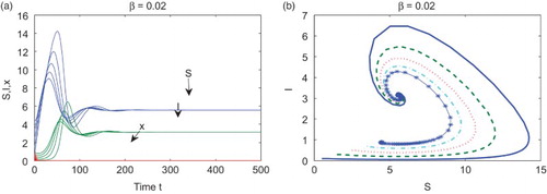
First, set $\mathrm{\Lambda }=0.4$, $r=0.9$, $\delta =0.8$, $\tau =1.25$, $\beta =0.001$, $\mu =0.01$, and $\gamma =0.1$. Then ${\mathcal{R}}_0=0.3591<1$. By Theorem 4.2, $E_2$ attracts all solutions with initial conditions in $\left\{\right(S,i,x)\in \mathrm{\Gamma }:x\in [0,1\left)\right\}$. Figure 1(a) supports this with the initial condition $(S_0,i_0,x_0)=(0.5,50{\mathrm{e}}^{-.4a},0.1)$. In Figure 1(b), we plot the phase diagram in the SI-plane with five different initial conditions.

Figure 1. With $\mathrm{\Lambda }=0.4$, $r=0.9$, $\delta =0.8$, $\tau =1.25$, $\beta =0.001$, $\mu =0.01$, and $\gamma =0.1$, the equilibrium $E_2$ attracts all solutions with initial conditions in $\left\{\right(S,i,x)\in \mathrm{\Gamma }:x\in [0,1\left)\right\}$. (a) Time series of S, I, and x with five different initial conditions; (b) the phase diagram in the SI-plane with five different initial conditions.

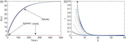
Second, enlarge the transmission rate to $\beta =0.02$ while keeping the other parameters at the same values as in the first case. Then ${\mathcal{R}}_0=7.1824$, which is between 1 and $1+r/\mu =91$. It follows from Theorems 3.2 and 4.3 that the endemic and vaccinator equilibrium $E_3$ is globally asymptotically stable. Figure 2 indicates that Equation (3(3) $\begin{array}{rl}& \frac{\mathrm{d}S\left(t\right)}{\mathrm{d}t}=\mathrm{\Lambda }(1-x)-S\left(t\right){\int }_0^{\mathrm{\infty }}\beta \left(a\right)i(t,a)\mathrm{d}a-\mu S\left(t\right),\\ & \frac{\mathrm{\partial }i(t,a)}{\mathrm{\partial }t}+\frac{\mathrm{\partial }i(t,a)}{\mathrm{\partial }a}=-(\mu +\gamma (a\left)\right)i(t,a),\\ & \frac{\mathrm{d}x\left(t\right)}{\mathrm{d}t}=\delta x(1-x)\left({\int }_0^{\mathrm{\infty }}\beta \left(a\right)i(t,a)\mathrm{d}a-r\right)\end{array}$(3) ) evolves towards $E_3$.

Figure 2. With $\mathrm{\Lambda }=0.4$, $r=0.9$, $\delta =0.8$, $\tau =1.25$, $\beta =0.02$, $\mu =0.01$, and $\gamma =0.1$, the equilibrium $E_3$ is locally asymptotically stable. (a) Times series of S (blue), I (green), and x (red) with five different initial conditions, (b) the corresponding phase diagram in the SI-plane.

Suppose the cost for the vaccination is too small and let $r=0.000001$. From the third equation of (3(3) $\begin{array}{rl}& \frac{\mathrm{d}S\left(t\right)}{\mathrm{d}t}=\mathrm{\Lambda }(1-x)-S\left(t\right){\int }_0^{\mathrm{\infty }}\beta \left(a\right)i(t,a)\mathrm{d}a-\mu S\left(t\right),\\ & \frac{\mathrm{\partial }i(t,a)}{\mathrm{\partial }t}+\frac{\mathrm{\partial }i(t,a)}{\mathrm{\partial }a}=-(\mu +\gamma (a\left)\right)i(t,a),\\ & \frac{\mathrm{d}x\left(t\right)}{\mathrm{d}t}=\delta x(1-x)\left({\int }_0^{\mathrm{\infty }}\beta \left(a\right)i(t,a)\mathrm{d}a-r\right)\end{array}$(3) ) we know that x monotonously increases to 1. Then Equation (3(3) $\begin{array}{rl}& \frac{\mathrm{d}S\left(t\right)}{\mathrm{d}t}=\mathrm{\Lambda }(1-x)-S\left(t\right){\int }_0^{\mathrm{\infty }}\beta \left(a\right)i(t,a)\mathrm{d}a-\mu S\left(t\right),\\ & \frac{\mathrm{\partial }i(t,a)}{\mathrm{\partial }t}+\frac{\mathrm{\partial }i(t,a)}{\mathrm{\partial }a}=-(\mu +\gamma (a\left)\right)i(t,a),\\ & \frac{\mathrm{d}x\left(t\right)}{\mathrm{d}t}=\delta x(1-x)\left({\int }_0^{\mathrm{\infty }}\beta \left(a\right)i(t,a)\mathrm{d}a-r\right)\end{array}$(3) ) has a pure vaccinator equilibrium $E_1$, which is unstable by Theorem 3.2 (see Figure 3(a)). if the cost of the vaccination is free or low, then the coverage of the proportion vaccinated is towards high values. However, persons have no incentives to vaccinate and the pure vaccinator equilibrium is unstable.

Figure 3. Representative time series of S (blue), I (green), and x (red). (a) $E_1$ is unstable, here $\mathrm{\Lambda }=0.4$, $r=0.000001$, $\delta =0.5$, $\tau =1.25$, $\beta =0.005$, $\mu =1/50\times 365$, and $\gamma =0.1$; (b) $E_4$ is locally asymptotically stable with $\mathrm{\Lambda }=0.4$, $r=0.01$, $\delta =0.5$, $\tau =1.25$, $\beta =0.005$, $\mu =1/50\times 365$, and $\gamma =0.1$.

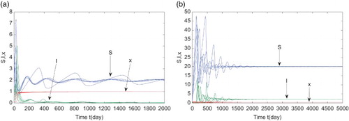
We rise the cost for vaccination to $r=0.01$ (which is between $0.000001$ (lower cost) and $1.2$ (higher cost)) and keep the other parameters unchanged as in the second case. Note that $\delta =0.5<1<\beta \mathrm{\Lambda }/\beta \mathrm{\Lambda }-(\mu +\gamma )(\mu +r)$. Theorem 3.2 implies that the endemic and vaccinator equilibrium $E_4$ is locally asymptotically stable, which is supported in Figure 3(b).

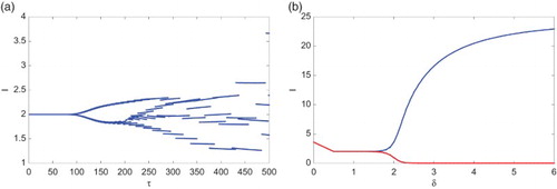
Theorem 3.2, Proposition 3.5, and Theorem 3.6 imply that δ, τ, and r play an important role in the evolution of (3(3) $\begin{array}{rl}& \frac{\mathrm{d}S\left(t\right)}{\mathrm{d}t}=\mathrm{\Lambda }(1-x)-S\left(t\right){\int }_0^{\mathrm{\infty }}\beta \left(a\right)i(t,a)\mathrm{d}a-\mu S\left(t\right),\\ & \frac{\mathrm{\partial }i(t,a)}{\mathrm{\partial }t}+\frac{\mathrm{\partial }i(t,a)}{\mathrm{\partial }a}=-(\mu +\gamma (a\left)\right)i(t,a),\\ & \frac{\mathrm{d}x\left(t\right)}{\mathrm{d}t}=\delta x(1-x)\left({\int }_0^{\mathrm{\infty }}\beta \left(a\right)i(t,a)\mathrm{d}a-r\right)\end{array}$(3) ). Recall that δ represents the imitation rate describing the imitated behaviours and the vaccination behaviour for children is determined by the imitation rate. Let $\mathrm{\Lambda }=0.4$, $r=0.01$, $\tau =1.25$, $\beta =0.05$, $\mu =\frac{1}{50\times 365}$, and $\gamma =0.1$. For some larger imitation rate δ, system (3(3) $\begin{array}{rl}& \frac{\mathrm{d}S\left(t\right)}{\mathrm{d}t}=\mathrm{\Lambda }(1-x)-S\left(t\right){\int }_0^{\mathrm{\infty }}\beta \left(a\right)i(t,a)\mathrm{d}a-\mu S\left(t\right),\\ & \frac{\mathrm{\partial }i(t,a)}{\mathrm{\partial }t}+\frac{\mathrm{\partial }i(t,a)}{\mathrm{\partial }a}=-(\mu +\gamma (a\left)\right)i(t,a),\\ & \frac{\mathrm{d}x\left(t\right)}{\mathrm{d}t}=\delta x(1-x)\left({\int }_0^{\mathrm{\infty }}\beta \left(a\right)i(t,a)\mathrm{d}a-r\right)\end{array}$(3) ) exhibits limit cycles and hence it can be destabilized by the imitation rate δ. Figure 4(a) shows the bifurcation diagram by taking δ as a bifurcation parameter, which indicates that the amplitude of the oscillations increases as the imitation rate does; while Figure 4(b) shows the phase diagram in the Ix-plane with $\delta =0.5$, $1.5$, and $2.5$, and the initial condition $(S_0,i_0,x_0)=(0.5,5{\mathrm{e}}^{-0.4a},0.1)$.

Figure 4. With $\mathrm{\Lambda }=0.4$, $r=0.01$, $\tau =1.25$, $\beta =0.05$, $\mu =1/50\times 365$, and $\gamma =0.1$, the imitation rate δ can destabilize (3(3) $\begin{array}{rl}& \frac{\mathrm{d}S\left(t\right)}{\mathrm{d}t}=\mathrm{\Lambda }(1-x)-S\left(t\right){\int }_0^{\mathrm{\infty }}\beta \left(a\right)i(t,a)\mathrm{d}a-\mu S\left(t\right),\\ & \frac{\mathrm{\partial }i(t,a)}{\mathrm{\partial }t}+\frac{\mathrm{\partial }i(t,a)}{\mathrm{\partial }a}=-(\mu +\gamma (a\left)\right)i(t,a),\\ & \frac{\mathrm{d}x\left(t\right)}{\mathrm{d}t}=\delta x(1-x)\left({\int }_0^{\mathrm{\infty }}\beta \left(a\right)i(t,a)\mathrm{d}a-r\right)\end{array}$(3) ). (a) The bifurcation diagram showing I with respect to the imitation rate δ with δ varying from 0 to 6; (b) representative phase diagram in the Ix-plane with δ being $0.5$(blue), $1.5$(green), and $2.5$(red), respectively, and the same initial condition $(S_0,i_0,x_0)=(0.5,5{\mathrm{e}}^{-0.4a},0.1)$.

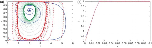
The perceived vaccine risk r impacts the prevalence of the disease spread. If the cost of the vaccination is high, such as a vaccine scare or a strong side effect, the frequency of the vaccination will gradually decrease and the prevalence of the disease will increase. Figure 5(a) shows the infection equilibrium structure of (3(3) $\begin{array}{rl}& \frac{\mathrm{d}S\left(t\right)}{\mathrm{d}t}=\mathrm{\Lambda }(1-x)-S\left(t\right){\int }_0^{\mathrm{\infty }}\beta \left(a\right)i(t,a)\mathrm{d}a-\mu S\left(t\right),\\ & \frac{\mathrm{\partial }i(t,a)}{\mathrm{\partial }t}+\frac{\mathrm{\partial }i(t,a)}{\mathrm{\partial }a}=-(\mu +\gamma (a\left)\right)i(t,a),\\ & \frac{\mathrm{d}x\left(t\right)}{\mathrm{d}t}=\delta x(1-x)\left({\int }_0^{\mathrm{\infty }}\beta \left(a\right)i(t,a)\mathrm{d}a-r\right)\end{array}$(3) ) in terms of the disease prevalence vs. r with $\mathrm{\Lambda }=0.4$, $\delta =0.5$, $\tau =1.25$, $\beta =0.05$, $\mu =1/50\times 365$, and $\gamma =0.1$. We can see that the disease prevalence increases when the cost of vaccination increases. Moreover, the equilibrium $E_4$ changes stability with r in the interval $[0,0.2]$ at $r=0.01$ from stable to unstable.

Figure 5. With $\mathrm{\Lambda }=0.4$, $\delta =0.5$, $\beta =0.05$, $\mu =1/50\times 365$, and $\gamma =0.1$, (a) infection equilibrium structure of (3(3) $\begin{array}{rl}& \frac{\mathrm{d}S\left(t\right)}{\mathrm{d}t}=\mathrm{\Lambda }(1-x)-S\left(t\right){\int }_0^{\mathrm{\infty }}\beta \left(a\right)i(t,a)\mathrm{d}a-\mu S\left(t\right),\\ & \frac{\mathrm{\partial }i(t,a)}{\mathrm{\partial }t}+\frac{\mathrm{\partial }i(t,a)}{\mathrm{\partial }a}=-(\mu +\gamma (a\left)\right)i(t,a),\\ & \frac{\mathrm{d}x\left(t\right)}{\mathrm{d}t}=\delta x(1-x)\left({\int }_0^{\mathrm{\infty }}\beta \left(a\right)i(t,a)\mathrm{d}a-r\right)\end{array}$(3) ) with $\tau =1.25$; (b) bifurcation diagram with the latent period τ as bifurcation parameter and $r=0.01$.

The latent period τ is also a key parameter for controlling the disease. For a childhood disease, if some medicine can extend the latent period of the disease, the prevalence of the disease can be lowered. Figure 5(b) shows that τ can destabilize (3(3) $\begin{array}{rl}& \frac{\mathrm{d}S\left(t\right)}{\mathrm{d}t}=\mathrm{\Lambda }(1-x)-S\left(t\right){\int }_0^{\mathrm{\infty }}\beta \left(a\right)i(t,a)\mathrm{d}a-\mu S\left(t\right),\\ & \frac{\mathrm{\partial }i(t,a)}{\mathrm{\partial }t}+\frac{\mathrm{\partial }i(t,a)}{\mathrm{\partial }a}=-(\mu +\gamma (a\left)\right)i(t,a),\\ & \frac{\mathrm{d}x\left(t\right)}{\mathrm{d}t}=\delta x(1-x)\left({\int }_0^{\mathrm{\infty }}\beta \left(a\right)i(t,a)\mathrm{d}a-r\right)\end{array}$(3) ) and oscillations occur when τ is from 100 to 500. Here $r=0.01$ and the other parameters except τ have the same values as above for the impact of r. Also, the prevalence of the disease gradually increases with respect to τ.

6. Discussion

From the theoretical analysis in the above sections, the pure vaccinator equilibrium $E_1$ is always unstable. Parents have no incentive to vaccinate if the vaccination coverage is high. The disease free and non-vaccinator equilibrium $E_2$ is globally asymptotically stable if and only if ${\mathcal{R}}_0<1$. If $1<{\mathcal{R}}_0$, then there is an endemic and non-vaccinator equilibrium $E_3$, which is locally asymptotically stable if $1<{\mathcal{R}}_0<1+\mu /r$. The endemic and vaccinator equilibrium $E_4$ is locally asymptotically stable if ${\mathcal{R}}_0>1+\mu /r$, $\delta <\mathrm{\Lambda }\beta /(\beta \mathrm{\Lambda }-(\mu +\gamma \left)\right(\mu +r\left)\right)$ and $\mathbb{S}=\mathrm{\varnothing }$. If $\mathbb{S}=\{{\tau }_0,\dots ,{\tau }_{n_0}\}$ with $s_{n\left({\tau }_0\right)}\left({\tau }_0\right)>0$, then a Hopf bifurcation occurs from the equilibrium $E_4$, which implies that Equation (3(3) $\begin{array}{rl}& \frac{\mathrm{d}S\left(t\right)}{\mathrm{d}t}=\mathrm{\Lambda }(1-x)-S\left(t\right){\int }_0^{\mathrm{\infty }}\beta \left(a\right)i(t,a)\mathrm{d}a-\mu S\left(t\right),\\ & \frac{\mathrm{\partial }i(t,a)}{\mathrm{\partial }t}+\frac{\mathrm{\partial }i(t,a)}{\mathrm{\partial }a}=-(\mu +\gamma (a\left)\right)i(t,a),\\ & \frac{\mathrm{d}x\left(t\right)}{\mathrm{d}t}=\delta x(1-x)\left({\int }_0^{\mathrm{\infty }}\beta \left(a\right)i(t,a)\mathrm{d}a-r\right)\end{array}$(3) ) can be destabilized. From the biological perspective, the childhood diseases are controlled if the transmission rates are small enough; Otherwise, the diseases will spread and become endemic diseases in some region. Moreover, if vaccination payoff is high, parents have a heavy burden from vaccinating their children, then they would avoid vaccinating their children and this leads to the spread of childhood diseases. If the vaccination payoff is not large enough and the total sampling rate for non-vaccinators imitating vaccinators is small enough, even if some of the parents would vaccinate their children, childhood diseases still spread in these areas. If, however, the sampling rate for non-vaccinators imitating vaccinators is large enough, this will lead to imitating phenomena switching, i.e, first, non-vaccinators imitating vaccinators decreases, and then the vaccination side effects will increase; Hence, vaccinators imitating non-vaccinators increases, and then the diseases will spread. Then the phenomenon will continue to cycle.

The imitation rate δ is the main parameter that leads to destabilization of the system and to a Hopf bifurcation, which is proved in [2, 12]. The amplitude of the oscillation increases with the increase of the imitated behaviours. As mentioned earlier in Section 5, individuals imitate others more readily as the amount of information for the significant side effects of vaccination increases, which in turn enhances the difficulties in disease control. The differences in infectivity, involved in childhood diseases, is incorporated through $\beta \left(a\right)$, the different transmission ability for the different values of the infection age a. For special cases, the different transmissibility can be described by the parameters τ and β. Suitable higher value of τ will produce a limit cycle.

When there is no cost for vaccination, that is, $r=0$, the payoff benefit is larger than the cost of vaccination as long as ${\int }_0^{\mathrm{\infty }}\beta \left(a\right)i(t,a)\mathrm{d}a$ is not zero. From the third equation of (3(3) $\begin{array}{rl}& \frac{\mathrm{d}S\left(t\right)}{\mathrm{d}t}=\mathrm{\Lambda }(1-x)-S\left(t\right){\int }_0^{\mathrm{\infty }}\beta \left(a\right)i(t,a)\mathrm{d}a-\mu S\left(t\right),\\ & \frac{\mathrm{\partial }i(t,a)}{\mathrm{\partial }t}+\frac{\mathrm{\partial }i(t,a)}{\mathrm{\partial }a}=-(\mu +\gamma (a\left)\right)i(t,a),\\ & \frac{\mathrm{d}x\left(t\right)}{\mathrm{d}t}=\delta x(1-x)\left({\int }_0^{\mathrm{\infty }}\beta \left(a\right)i(t,a)\mathrm{d}a-r\right)\end{array}$(3) ), the frequency of vaccination monotonously increases. It follows from the first two equations combined with the third equation of (3(3) $\begin{array}{rl}& \frac{\mathrm{d}S\left(t\right)}{\mathrm{d}t}=\mathrm{\Lambda }(1-x)-S\left(t\right){\int }_0^{\mathrm{\infty }}\beta \left(a\right)i(t,a)\mathrm{d}a-\mu S\left(t\right),\\ & \frac{\mathrm{\partial }i(t,a)}{\mathrm{\partial }t}+\frac{\mathrm{\partial }i(t,a)}{\mathrm{\partial }a}=-(\mu +\gamma (a\left)\right)i(t,a),\\ & \frac{\mathrm{d}x\left(t\right)}{\mathrm{d}t}=\delta x(1-x)\left({\int }_0^{\mathrm{\infty }}\beta \left(a\right)i(t,a)\mathrm{d}a-r\right)\end{array}$(3) ) that system (3(3) $\begin{array}{rl}& \frac{\mathrm{d}S\left(t\right)}{\mathrm{d}t}=\mathrm{\Lambda }(1-x)-S\left(t\right){\int }_0^{\mathrm{\infty }}\beta \left(a\right)i(t,a)\mathrm{d}a-\mu S\left(t\right),\\ & \frac{\mathrm{\partial }i(t,a)}{\mathrm{\partial }t}+\frac{\mathrm{\partial }i(t,a)}{\mathrm{\partial }a}=-(\mu +\gamma (a\left)\right)i(t,a),\\ & \frac{\mathrm{d}x\left(t\right)}{\mathrm{d}t}=\delta x(1-x)\left({\int }_0^{\mathrm{\infty }}\beta \left(a\right)i(t,a)\mathrm{d}a-r\right)\end{array}$(3) ) evolves to $E_2$. On the other hand, if the cost of vaccination is not free, and the initial conditions satisfy ${\int }_0^{\mathrm{\infty }}\beta \left(a\right)i(t_0,a)\mathrm{d}a>r$, the frequency of the vaccination monotonously increases. It follows from the first and second equation of (3(3) $\begin{array}{rl}& \frac{\mathrm{d}S\left(t\right)}{\mathrm{d}t}=\mathrm{\Lambda }(1-x)-S\left(t\right){\int }_0^{\mathrm{\infty }}\beta \left(a\right)i(t,a)\mathrm{d}a-\mu S\left(t\right),\\ & \frac{\mathrm{\partial }i(t,a)}{\mathrm{\partial }t}+\frac{\mathrm{\partial }i(t,a)}{\mathrm{\partial }a}=-(\mu +\gamma (a\left)\right)i(t,a),\\ & \frac{\mathrm{d}x\left(t\right)}{\mathrm{d}t}=\delta x(1-x)\left({\int }_0^{\mathrm{\infty }}\beta \left(a\right)i(t,a)\mathrm{d}a-r\right)\end{array}$(3) ) that infected individuals decrease until ${\int }_0^{\mathrm{\infty }}\beta \left(a\right)i^{\ast }\left(a\right)\mathrm{d}a=r$. System (3(3) $\begin{array}{rl}& \frac{\mathrm{d}S\left(t\right)}{\mathrm{d}t}=\mathrm{\Lambda }(1-x)-S\left(t\right){\int }_0^{\mathrm{\infty }}\beta \left(a\right)i(t,a)\mathrm{d}a-\mu S\left(t\right),\\ & \frac{\mathrm{\partial }i(t,a)}{\mathrm{\partial }t}+\frac{\mathrm{\partial }i(t,a)}{\mathrm{\partial }a}=-(\mu +\gamma (a\left)\right)i(t,a),\\ & \frac{\mathrm{d}x\left(t\right)}{\mathrm{d}t}=\delta x(1-x)\left({\int }_0^{\mathrm{\infty }}\beta \left(a\right)i(t,a)\mathrm{d}a-r\right)\end{array}$(3) ) evolves to the endemic and non-vaccinator equilibrium $E_3$ or a stable endemic and vaccinator equilibrium $E_4$ which depends on whether the initial vaccinated proportion is equal or larger than 0. When ${\int }_0^{\mathrm{\infty }}\beta \left(a\right)i(t,a)\mathrm{d}a<r$, it follows from the third equation of (3(3) $\begin{array}{rl}& \frac{\mathrm{d}S\left(t\right)}{\mathrm{d}t}=\mathrm{\Lambda }(1-x)-S\left(t\right){\int }_0^{\mathrm{\infty }}\beta \left(a\right)i(t,a)\mathrm{d}a-\mu S\left(t\right),\\ & \frac{\mathrm{\partial }i(t,a)}{\mathrm{\partial }t}+\frac{\mathrm{\partial }i(t,a)}{\mathrm{\partial }a}=-(\mu +\gamma (a\left)\right)i(t,a),\\ & \frac{\mathrm{d}x\left(t\right)}{\mathrm{d}t}=\delta x(1-x)\left({\int }_0^{\mathrm{\infty }}\beta \left(a\right)i(t,a)\mathrm{d}a-r\right)\end{array}$(3) ) that the proportion vaccinated x decreases. Prevalence of the disease increases until ${\int }_0^{\mathrm{\infty }}\beta \left(a\right)i^{\ast }\left(a\right)\mathrm{d}a=r$. This implies that Equation (3(3) $\begin{array}{rl}& \frac{\mathrm{d}S\left(t\right)}{\mathrm{d}t}=\mathrm{\Lambda }(1-x)-S\left(t\right){\int }_0^{\mathrm{\infty }}\beta \left(a\right)i(t,a)\mathrm{d}a-\mu S\left(t\right),\\ & \frac{\mathrm{\partial }i(t,a)}{\mathrm{\partial }t}+\frac{\mathrm{\partial }i(t,a)}{\mathrm{\partial }a}=-(\mu +\gamma (a\left)\right)i(t,a),\\ & \frac{\mathrm{d}x\left(t\right)}{\mathrm{d}t}=\delta x(1-x)\left({\int }_0^{\mathrm{\infty }}\beta \left(a\right)i(t,a)\mathrm{d}a-r\right)\end{array}$(3) ) also evolves to the endemic and non-vaccinator equilibrium $E_3$ or the endemic and vaccinator equilibrium $E_4$ which depends on the initial vaccinated proportion $x_0$.

In summary, parents can make rational decisions in favour of disease control if they understand the interplay between the perceived vaccination risk, prevalence of the disease, and the variable transmission abilities of the children. Our investigation implies that high vaccination coverage can not guarantee the elimination of the disease for a voluntary vaccination policy. On the other hand, limited vaccination may be harmful for control of the disease spread. The amount of up-to-date information for the vaccine use has two opposite effects: knowledge about the disease prevalence encourages parents to take the vaccine for their children, on the other hand the potential side effects discourage them to take vaccine for their children. Rational decision-making individuals, depending on updated information about the perceived vaccine risk compared with the prevalence of the disease, decide whether or not to vaccinate their children. Based on the game theory, we conclude that it is important that parents make rational decision whether or not to vaccinate their children.

Disclosure statement

No potential conflict of interest was reported by the authors.

Additional information

Funding

Research is supported partially by the National Natural Science Foundation of China (61573016, 61203228, 11371313), China Scholarship Council (201308140016), the Young Sciences Foundation of Shanxi (2011021001-1), Program for the Outstanding Innovative Teams of Higher Learning Institutions of Shanxi, ‘131’ Talents of Shanxi University, the Natural Sciences and Engineering Research Council (NSERC) of Canada, and the NSF DMS-1220342, DMS-1515661 grants.

References

- N.E. Basta, D.L. Chao, M.E. Halloran, and I.M. Longini Jr, Strategies for pandemic and seasonal influenza vaccination of schoolchildren in the United States, Am. J. Epidemiol. 170(6) (2009), pp. 679–686. doi: 10.1093/aje/kwp237
- C.T. Bauch, Imitation dynamics predict vaccinating behaviour, Proc R. Soc. B 272(1573) (2005), pp. 1669–1675. doi: 10.1098/rspb.2005.3153
- C.T. Bauch and D.J.D. Earn, Vaccination and the theory of games, Proc. Natl Acad. Sci. USA 101 (2004), pp. 13391–13394. doi: 10.1073/pnas.0403823101
- E. Beretta and Y. Kuang, Geometric stability switch criteria in delay differential systems with delay dependent parameters, SIAM J. Math. Anal. 33(5) (2002), pp. 1144–1165. doi: 10.1137/S0036141000376086
- S.R. Boëlle, Modelling the effects of population structure on childhood disease: The case of varicella, PLoS Comput. Biol. 7(7) (2011), p. e1002105. doi: 10.1371/journal.pcbi.1002105.
- C.J. Browne and S.S. Plyugin, Global analysis of age-structured within-host virus model, Discrete Contin. Dyn. Syst. Ser. B. 18(8) (2013), pp. 1999–2017. doi: 10.3934/dcdsb.2013.18.1999
- Centers for Disease Control and Prevention. CDC Health Information for International Travel 2014. Oxford University Press, New York, 2014.
- F.C. Coelho and C.T. Codeço, Dynamic modeling of vaccinating behavior as a function of individual beliefs, PLoS Comput. Biol. 5(7) (2009), p. e1000425. doi: 10.1371/journal.pcbi.1000425
- D.M. Cornforth, T.C. Reluga, E. Shim, C.T. Bauch, A.P. Galvani, and L.A. Meyers, Erratic flu vaccination emerges from short-sighted behaviour in contact networks, Plos Comput. Biol. 7(1) (2011), p. e1001062. doi: 10.1371/journal.pcbi.1001062
- R. Cressman, Evolutionary Dynamics and Extensive Form Games, MIT Press, Cambridge, MA, 2003.
- A. d'Onofrio and P. Manfredi, Vaccine demand driven by vaccine side effects: Dynamic implications for SIR diseases, J. Theoret. Biol. 264(2) (2010), pp. 237–252. doi: 10.1016/j.jtbi.2010.02.007
- A. d'Onofrio, P. Manfredi, and P. Poletti, The impact of vaccine side effects on the natural history of immunization programmes: An imitation-game approach, J. Theoret. Biol. 273(1) (2011), pp. 63–71. doi: 10.1016/j.jtbi.2010.12.029
- D.J.D. Earn, P. Rohani, B.M. Bolker, and B.T. Grenfell, A simple model for complex dynamical transitions in epidemics, Science 287 (2000), pp. 667–670. doi: 10.1126/science.287.5453.667
- E.P. Fenichel, C. Castillo-Chavez, M.G. Ceddia, G. Chowell, P.A. Parra, G.J. Hickling, G. Holloway, R. Horan, B. Morin, C. Perrings, M. Springborn, L. Velazquez, and C. Villalobos, Adaptive human behavior in epidemiological models, Proc. Natl. Acad. Sci. USA 108 (2011), pp. 6306–6311. doi: 10.1073/pnas.1011250108
- P.E.M. Fine and J.A. Clarkson, Individual versus public priorities in the determination of optimal vaccination policies, Am. J. Epidemiol. 124 (1986), pp. 1012–1020.
- B.F. Finkenstädt and B.T. Grenfell, Time series modelling of childhood diseases: A dynamical systems approach, J. Roy. Statist. Soc. Ser. C 49 (2000), pp. 187–205. doi: 10.1111/1467-9876.00187
- F. Fu, D.I. Rosenbloom, L. Wang, and M.A. Nowak, Imitation dynamics of vaccination behaviour on social networks, Proc. R. Soc. B 278 (2011), pp. 42–49. doi: 10.1098/rspb.2010.1107
- J.T. Griffin, N.M. Ferguson, and A.C. Ghani, Estimates of the changing age-burden of Plasmodium falciparum malaria disease in sub-Saharan Africa, Nat. Commun. 5:3136 (2014). doi:10.1038/ncomms4136.
- J.K. Hale, Asymptotic Behavior of Dissipative Systems, AMS, Providence, 1988.
- W.M. Hirsch, H. Hanisch, and J.-P . Gabriel, Differential equation models of some parasitic infections: Methods for the study of asymptotic behavior, Comm. Pure Appl. Math. 38 (1985), pp. 733–753. doi: 10.1002/cpa.3160380607
- M. Iannelli, Mathematical theory of age-structured population dynamics, in Applied Mathematics Monographs 7, comitato Nazionale per le Scienze Matematiche, Consiglio Nazionale delle Ricerche (C.N.R.), Giardini, Pisa, 1995.
- N.B. Kandala, T.P. Madungu, J.B.O. Emina, K.P.D. Nzita, and F.P. Cappuccio, Malnutrition among children under the age of five in the Democratic Republic of Congo (DRC): Does geographic location matter? BMC Public Health 11 (2011), pp. 261–276. doi: 10.1186/1471-2458-11-261
- P. Magal, Compact attractors for time periodic age-structured population models, Electron. J. Differ. Equ. 65 (2001), pp. 1–35.
- P. Magal, C.C. McCluskey, and G.F. Webb, Lyapunov functional and global asymptotic stability for an infection-age model, Appl. Anal. 89 (2010), pp. 1109–1140. doi: 10.1080/00036810903208122
- C.J.E. Metcalf, J. Lessler, P. Klepac, F. Cutts, and B.T. Grenfell, Impact of birth rate, seasonality and transmission rate on minimum levels of coverage needed for rubella vaccination, Epidemiol. Infect. 140(12) (2012), pp. 2290–2301. doi: 10.1017/S0950268812000131
- National Center for Immunization and Respiratory Diseases (NCIRD). Available at http://www.cdc.gov/mumps/clinical/qa-disease.html.
- Pertussis (Whooping Cough): Questions and Answers. Available at http://www.immunize.org/catg.d/p4212.pdf.
- T.C. Reluga and A.P. Galvani, A general approach for population games with application to vaccination, Math. Biosci. 230(2) (2011), pp. 67–78. doi: 10.1016/j.mbs.2011.01.003
- D. Schenzle, An age-structured model of pre- and post-vaccination measles transmission, Math. Med. Biol. 1 (1984), pp. 169–191. doi: 10.1093/imammb/1.2.169
- E. Shim, G.B. Chapman, and A.P. Galvani, Decision making with regard to antiviral intervention during an influenza pandemic, Med. Decis. Making 30(4) (2010), p. E64-81.
- E. Shim, J.J. Grefenstette, S.M. Albert, B.E. Cakouros, and D.S. Burke, A game dynamic model for vaccine skeptics and vaccine believers: Measles as an example, J. Theoret. Biol. 295 (2012), pp. 194–203. doi: 10.1016/j.jtbi.2011.11.005
- E. Shim, B. Kochin, and A.P. Galvani, Insights from epidemiological game theory into gender-specific vaccination against rubella, Math. Biosci. Eng. 6(4) (2009), pp. 893–854. doi: 10.3934/mbe.2009.6.839
- R.H. Thieme, Uniform persistence and permanence for non-autonomous semiflows in population biology, Math. Biosci. 166 (2000), pp. 173–201. doi: 10.1016/S0025-5564(00)00018-3
- D. Weycker, J. Edelsberg, M.E. Halloran, I.M. Longini, A. Nizam, V. Ciuryla, and G. Oster, Population-wide benefits of routine vaccination of children against influenza, Vaccine 23(10) (2005), pp. 1284–1293. doi: 10.1016/j.vaccine.2004.08.044
- S. Xia and J. Liu, A computational approach to characterizing the impact of social influence on individuals' vaccination decision making, PLoSONE. 8(4) (2013), p. e60373. doi: 10.1371/journal.pone.0060373.
- S. Xia and J. Liu, A belief-based model for characterizing the spread of awareness and its impacts on individuals' vaccination decisions, J. R. Soc. B 11 (2014), p. 20140013.
- S. Xia, J. Liu, and W. Cheung, Identifying the relative priorities of subpopulations for containing infectious disease spread, PLoS ONE. 8(6) (2013), p. e65271. doi: 10.1371/journal.pone.0065271.
- F. Xu and R. Cressman, Disease control through voluntary vaccination decisions based on the smoothed best response, Comput. Math. Methods Med. (2014), Art. ID 825734, 14pp. doi:10.1155/2014/825734.
- K. Yasida, Functional Analysis, 2nd ed., Springer-Verlag, Berlin-Heidelberg, 1968.
- H. Zhang, F. Fu, W. Zhang, and B. Wang, Rational behavior is a ‘double-edged sword’ when considering voluntary vaccination, Phys. A 391 (2012), pp. 4807–4815. doi: 10.1016/j.physa.2012.05.009