Full article: Dynamics of low and high pathogenic avian influenza in wild and domestic bird populations

Formulae display: $MathJax Logo$ ?Mathematical formulae have been encoded as MathML and are displayed in this HTML version using MathJax in order to improve their display. Uncheck the box to turn MathJax off. This feature requires Javascript. Click on a formula to zoom.

ABSTRACT

This paper introduces a time-since-recovery structured, multi-strain, multi-population model of avian influenza. Influenza A viruses infect many species of wild and domestic birds and are classified into two groups based on their ability to cause disease: low pathogenic avian influenza (LPAI) and high pathogenic avian influenza (HPAI). Prior infection with LPAI provides partial immunity towards HPAI. The model introduced in this paper structures LPAI-recovered birds (wild and domestic) with time-since-recovery and includes cross-immunity towards HPAI that can fade with time. The model has a unique disease-free equilibrium (DFE), unique LPAI-only and HPAI-only equilibria and at least one coexistence equilibrium. We compute the reproduction numbers of LPAI ( $R_{L}$ ) and HPAI ( $R_{H}$ ) and show that the DFE is locally asymptotically stable when $R_{L} < 1$ and $R_{H} < 1$ . A unique LPAI-only (HPAI-only) equilibrium exists when $R_{L} > 1$ ( $R_{H} > 1$ ) and it is locally asymptotically stable if HPAI (LPAI) cannot invade the equilibrium, that is, if the invasion number ${\hat{R}}_{L}^{H} < 1$ ( ${\hat{R}}_{H}^{L} < 1$ ). We show using numerical simulations that the ODE version of the model, which is obtained by discarding the time-since-recovery structures (making cross-immunity constant), can exhibit oscillations, and also that the pathogens LPAI and HPAI can coexist with sustained oscillations in both populations. Through simulations, we show that even if both populations (wild and domestic) are sinks when alone, LPAI and HPAI can persist in both populations combined. Thus, reducing the reproduction numbers of LPAI and HPAI in each population to below unity is not enough to eradicate the disease. The pathogens can continue to coexist in both populations unless transmission between the populations is reduced.

KEYWORDS:

AMS SUBJECT CLASSIFICATIONS:

1. Introduction

Infectious disease dynamics often occur within the context of complex ecological communities [Citation9]. Moreover, many important host–pathogen systems consist of multiple pathogen strains, circulating among multiple species of hosts [7]. Understanding how multi-species transmission affects the persistence of a given pathogen strain can help inform prediction and management of infectious disease outbreaks, and understanding how such transmission among hosts modulates the coexistence of pathogen strains and thus the maintenance of genetic variation within pathogens is essential for gauging how pathogens are likely to evolve. This community dimension of epidemiology is widely recognized as being a significant frontier in quantitative epidemiology and the public health sciences [Citation10].

These issues arise with particular urgency in the case of the avian influenza viruses (AIVs), which present a global economic problem in the poultry industry costing annually hundreds of millions of dollars [Citation16] and pose a serious public health risk due to the threat of emergence of a novel pathogen strain circulating among human hosts, with potentially devastating consequences [Citation24]. Influenza A viruses can infect many species of warm-blooded vertebrates [Citation26], but the great majority of viral strains appear to be found in wild waterbirds, such as shorebirds and gulls (Charadriiformes) and ducks and geese (Anseriformes) [Citation12]. These species can come into contact with domestic poultry, which can pose a direct threat to the poultry industry, and also provide a conduit for potential transmission to humans.

Mathematical models can provide essential tools for understanding many aspects of infectious disease dynamics [Citation10], and become particularly important when grappling with the complexities of multi-pathogen, multi-host systems, for instance when hosts themselves may mount strain-specific immune responses to infection. A realistic model of avian influenza (AI) would be highly complex, since it would have to account for transmission within and among multiple potential species of wild hosts, many of which are migratory [Citation21] and occupy seasonally forced environments [Citation24]. As a way station towards such a realistic model, here we consider a system in which there are two host populations, which we call domestic and wild bird populations, each of which has relatively simple intrinsic dynamics. These two host populations are in turn infected by two strains of AI A, one of which is a strain of low pathogenic avian influenza (LPAI), and the other a strain of high pathogenic avian influenza (HPAI). HPAI viruses are defined by the fact that they cause at least 75% mortality in 4–8 week chickens, infected intravenously [Citation20]. HPAI strains are of influenza A subtypes H5 and H7 (e.g. H5N1, H7N9).

The basic dynamics of each host consists of a steady flow of fresh susceptibles into each host population, and a constant rate of intrinsic mortality. In the absence of the virus, the hosts have very stable dynamics. (This assumption would need to be relaxed when considering the detailed dynamics of natural populations, which fluctuate seasonally and among years.) Transmission of the virus occurs in a density-dependent fashion, both within and between these two populations. Hosts can recover from infection with LPAI, and when they do recover, are immune for life from further infection by this viral strain. However, LPAI-recovered birds can be infected by HPAI. Consistent with empirical evidence, there is a degree of cross-protection in the immune response, so infection by LPAI can protect against HPAI. However, this cross-immunity fades with time, and incorporating the dynamics of such time-dependent fade-out in immune protection is one of the mathematical complexities of our model. By contrast, infection with HPAI is assumed to always lead to death (possibly by culling) in domestic birds; in wild birds, HPAI leads to death or recovery with permanent immunity to both strains.

Our focus will be on the implications of partial cross-immunity, but to put our results into context, it is useful to consider what might be expected when cross-immunity is complete. If cross-immunity is complete, then LPAI and HPAI simply compete for susceptible hosts. If there is only one population, within which each strain could persist alone, whichever strain can persist at the lowest level of susceptibles will eliminate the other strain. With two populations, there are two resources (the susceptibles in the two populations), so there are other possibilities. One is that the two strains coexist, for example if LPAI is better at exploiting wild susceptibles and HPAI is better at exploiting domestic susceptibles. Another possibility is that each strain can exclude the other, in which case the first strain to arrive persists and the second strain cannot invade (alternative equilibria). If cross-immunity is not complete, HPAI can infect at least some LPAI-recovered birds, and so it has an additional resource. Therefore, coexistence is possible in a single population if LPAI is better at exploiting susceptibles; with complete cross-immunity, LPAI would eliminate HPAI, but with partial cross-immunity, it is sometimes possible for HPAI to invade and persist by infecting LPAI-recovered birds. With two populations, of course, there is additional scope for coexistence. The analyses and simulations presented below help illuminate the conditions that permit such coexistence.

We first present the basic model (for a flow chart of the model, see Figure ). Then, we characterize the conditions for each viral strain to be able to increase when rare and alone. We derive expressions for the basic reproduction number for each strain, which are functions of the joint densities of the domestic and wild bird populations. Next, we consider the conditions for the increase of each strain when rare, when the other strain is present, and aim at characterizing conditions for the coexistence of the two strains. Such coexistence is not guaranteed. The two viral strains can be viewed as interacting in two distinct ways. Firstly, they compete exploitatively for healthy hosts. Given that there are two host populations, as noted above, there is the potential for a degree of niche partitioning that could facilitate viral strain coexistence [Citation9]. Secondly, the loss of partial immunity means there is a partial, time-lagged facilitation of the dynamics of HPAI, emerging from hosts who get infected with LPAI, but recover. This means that even if all hosts have been infected by LPAI (so no fully susceptible hosts are available at all), some hosts can become available for infection by HPAI.

Figure 1. Flow chart of model (Equation1(1) $\begin{aligned} \frac{d S_{w}}{d t} & = Λ_{w} - λ_{L_{w}} S_{w} - λ_{H_{w}} S_{w} - μ_{w} S_{w}, \\ \frac{d I_{L_{w}}}{d t} & = λ_{L_{w}} S_{w} - (μ_{w} + α_{L_{w}}) I_{L_{w}}, \\ \frac{\partial r_{L_{w}}}{\partial t} + \frac{\partial r_{L_{w}}}{\partial τ} & = - q_{w} (τ) λ_{H_{w}} r_{L_{w}} - μ_{w} r_{L_{w}}, \\ r_{L_{w}} (0, t) & = α_{L_{w}} I_{L_{w}}, \\ \frac{d I_{H_{w}}}{d t} & = λ_{H_{w}} S_{w} + λ_{H_{w}} \int_{0}^{\infty} q_{w} (τ) r_{L_{w}} (τ, t) d τ - (μ_{w} + α_{H_{w}} + ν_{H_{w}}) I_{H_{w}}, \\ \frac{d R_{H_{w}}}{d t} & = α_{H_{w}} I_{H_{w}} - μ_{w} R_{H_{w}}, \\ \frac{d S_{d}}{d t} & = Λ_{d} - λ_{L_{d}} S_{d} - λ_{H_{d}} S_{d} - μ_{d} S_{d}, \\ \frac{d I_{L_{d}}}{d t} & = λ_{L_{d}} S_{d} - (μ_{d} + α_{d}) I_{L_{d}}, \\ \frac{\partial r_{d}}{\partial t} + \frac{\partial r_{d}}{\partial τ} & = - q_{d} (τ) λ_{H_{d}} r_{d} - μ_{d} r_{d}, \\ r_{d} (0, t) & = α_{d} I_{L_{d}}, \\ \frac{d I_{H_{d}}}{d t} & = λ_{H_{d}} S_{d} + λ_{H_{d}} \int_{0}^{\infty} q_{d} (τ) r_{d} (τ, t) d τ - (μ_{d} + ν_{H_{d}}) I_{H_{d}} . \end{aligned}$ (1) ).

Figure 1. Flow chart of model (Equation1(1) dSwdt=Λw−λLwSw−λHwSw−μwSw,dILwdt=λLwSw−(μw+αLw)ILw,∂rLw∂t+∂rLw∂τ=−qw(τ)λHwrLw−μwrLw,rLw(0,t)=αLwILw,dIHwdt=λHwSw+λHw∫0∞qw(τ)rLw(τ,t)dτ−(μw+αHw+νHw)IHw,dRHwdt=αHwIHw−μwRHw,dSddt=Λd−λLdSd−λHdSd−μdSd,dILddt=λLdSd−(μd+αd)ILd,∂rd∂t+∂rd∂τ=−qd(τ)λHdrd−μdrd,rd(0,t)=αdILd,dIHddt=λHdSd+λHd∫0∞qd(τ)rd(τ,t)dτ−(μd+νHd)IHd.(1) ).

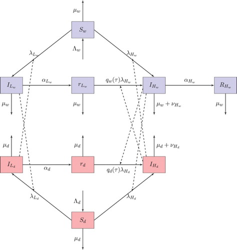
This replenishment of hosts for HPAI involves a lag, relative to LPAI infection. We will use numerical simulations to demonstrate that this permits the entire system to persist, but at times with sustained, large-scale oscillations in infection by each viral strain. Such oscillations can emerge even if each viral strain on its own tends towards a stable equilibrium when it alone is infecting the two host populations.

2. The model

We consider a time-since-recovery structured model to study the dynamics of LPAI and HPAI (indicated by L and H subscripts or superscripts, respectively) in wild and domestic bird populations (indicated by w or 1 subscripts for wild birds and d or 2 subscripts for domestic birds). The wild bird population is divided into nonintersecting classes of susceptible ( $S_{w}$ ), infected with HPAI ( $I_{H_{w}}$ ), infected with LPAI ( $I_{L_{w}}$ ), recovered from LPAI ( $r_{L_{w}}$ ), and recovered from HPAI ( $R_{H_{w}}$ ). Similarly, the domestic bird population is divided into susceptible ( $S_{d}$ ), infected with HPAI ( $I_{H_{d}}$ ), infected with LPAI ( $I_{L_{d}}$ ) and recovered from LPAI ( $r_{L_{d}}$ ) classes. Since the detection of even one HPAI-infected domestic bird results in culling the entire farm and the death of the infected bird, we do not include an HPAI-recovered class for the domestic bird population. The LPAI-recovered classes $r_{L_{w}} (τ, t)$ , $r_{L_{d}} (τ, t)$ denote the density of (per unit τ) recovered birds at time t with time-since-recovery equal to τ.

The susceptible bird populations are generated by the recruitment/birth rates ( $Λ_{w}$ and $Λ_{d}$ ) and reduced by the natural death rates ( $μ_{w}$ and $μ_{d}$ ) and by infection with HPAI or LPAI. The new infections with LPAI and HPAI, respectively, per unit time per susceptible host are modelled by $λ_{L_{w}}$ and $λ_{H_{w}}$ in wild birds. The forces of infection for LPAI and HPAI, respectively, in the wild bird population are given by $λ_{L_{w}} = β_{11}^{L} I_{L_{w}} + β_{12}^{L} I_{L_{d}}, λ_{H_{w}} = β_{11}^{H} I_{H_{w}} + β_{12}^{H} I_{H_{d}} .$ Similarly, the forces of infection for LPAI and HPAI, respectively, in the domestic bird population are given by $λ_{L_{d}} = β_{21}^{L} I_{L_{w}} + β_{22}^{L} I_{L_{d}}, λ_{H_{d}} = β_{21}^{H} I_{H_{w}} + β_{22}^{H} I_{H_{d}} .$

The aggregate β parameters can be interpreted as the product of rate of contacts between a susceptible (wild or domestic) bird and an infected (LPAI or HPAI) bird and the probability that the contact resulted in transmission. For instance, $β_{12}^{H}$ is the HPAI transmission rate to wild birds from domestic birds; similarly, $β_{21}^{L}$ is the LPAI transmission rate to domestic birds from wild birds (per susceptible bird per infected bird). Thus, the rate of change of the population of susceptible wild and domestic bird populations is given by $\begin{aligned} \frac{d S_{w}}{d t} & = Λ_{w} - λ_{L_{w}} S_{w} - λ_{H_{w}} S_{w} - μ_{w} S_{w}, \\ \frac{d S_{d}}{d t} & = Λ_{d} - λ_{L_{d}} S_{d} - λ_{H_{d}} S_{d} - μ_{d} S_{d} . \end{aligned}$ The infected wild birds recover from LPAI infection at a rate $α_{L_{w}}$ and the domestic birds recover at a rate $α_{d}$ . LPAI causes mild infection in domestic and wild birds (http://www.cdc.gov/flu/avianflu/avian-in-birds.htm), hence we neglect the LPAI-induced death rate. The LPAI-infected wild and domestic bird populations increase by the new incidences $λ_{L_{w}} S_{w}$ and $λ_{L_{d}} S_{d}$ , respectively. Thus, the wild and domestic bird populations infected with LPAI satisfy the following equations: $\begin{aligned} \frac{d I_{L_{w}}}{d t} & = λ_{L_{w}} S_{w} - (μ_{w} + α_{L_{w}}) I_{L_{w}}, \\ \frac{d I_{L_{d}}}{d t} & = λ_{L_{d}} S_{d} - (μ_{d} + α_{d}) I_{L_{d}} . \end{aligned}$ The HPAI-infected wild and domestic bird populations increase by the new incidences $λ_{H_{w}} S_{w}$ and $λ_{H_{d}} S_{d}$ , respectively. Wild birds infected with HPAI can recover at a rate $α_{H_{w}}$ ; domestic birds do not recover from HPAI. Studies show that an earlier infection with LPAI provides temporary immunity towards HPAI and this immunity fades with time-since-recovery from LPAI [Citation8, Citation18]. As τ is the time elapsed since the recovery from the last LPAI infection, the additional new HPAI infections per unit time from wild birds that have recovered from LPAI are given by the following term: $λ_{H_{w}} \int_{0}^{\infty} q_{w} (τ) r_{L_{w}} (τ, t) d τ,$ where $q_{w} (τ)$ is the susceptibility to HPAI of a wild bird that recovered from LPAI τ time units ago relative to that of a naive wild bird. Similarly, the new HPAI infections per unit time of the domestic birds recovered from LPAI infections are given by the following term: $λ_{H_{d}} \int_{0}^{\infty} q_{d} (τ) r_{d} (τ, t) d τ,$ where $q_{d} (τ)$ is the relative susceptibility to HPAI of an LPAI-recovered domestic bird. Thus, the wild and domestic bird populations infected with HPAI satisfy the following equations: $\begin{aligned} \frac{d I_{H_{w}}}{d t} & = λ_{H_{w}} S_{w} + λ_{H_{w}} \int_{0}^{\infty} q_{w} (τ) r_{L_{w}} (τ, t) d τ - (μ_{w} + α_{H_{w}} + ν_{H_{w}}) I_{H_{w}}, \\ \frac{d I_{H_{d}}}{d t} & = λ_{H_{d}} S_{d} + λ_{H_{d}} \int_{0}^{\infty} q_{d} (τ) r_{d} (τ, t) d τ - (μ_{d} + ν_{H_{d}}) I_{H_{d}}, \end{aligned}$ where $ν_{H_{w}}$ and $ν_{H_{d}}$ are disease death rates induced by HPAI in wild and domestic birds, respectively. We combine these differential equations with those for LPAI-recovered classes, $r_{L_{w}} (τ, t)$ and $r_{L_{d}} (τ, t)$ , which have relative susceptibilities to HPAI of $q_{w} (τ)$ and $q_{d} (τ)$ , respectively, where $0 \leq q_{w} (τ) \leq 1, 0 \leq q_{d} (τ) \leq 1$ for every $τ > 0$ . Thus, the differential equations modelling the recovered classes are $\begin{aligned} \frac{\partial r_{L_{w}}}{\partial t} + \frac{\partial r_{L_{w}}}{\partial τ} & = - q_{w} (τ) λ_{H_{w}} r_{L_{w}} - μ_{w} r_{L_{w}}, \\ r_{L_{w}} (0, t) & = α_{L_{w}} I_{L_{w}}, \\ \frac{\partial r_{d}}{\partial t} + \frac{\partial r_{d}}{\partial τ} & = - q_{d} (τ) λ_{H_{d}} r_{d} - μ_{d} r_{d}, \\ r_{d} (0, t) & = α_{d} I_{L_{d}} . \end{aligned}$ We note that in the above equations, we have assumed mass-action incidence. Since the contacts in influenza (avian or human) scale with the total population size, most influenza models are built with mass-action incidence [Citation1]. With the above notation, we have the following time-since-recovery structured, multi-strain, multi-population model: (1) $\begin{aligned} \frac{d S_{w}}{d t} & = Λ_{w} - λ_{L_{w}} S_{w} - λ_{H_{w}} S_{w} - μ_{w} S_{w}, \\ \frac{d I_{L_{w}}}{d t} & = λ_{L_{w}} S_{w} - (μ_{w} + α_{L_{w}}) I_{L_{w}}, \\ \frac{\partial r_{L_{w}}}{\partial t} + \frac{\partial r_{L_{w}}}{\partial τ} & = - q_{w} (τ) λ_{H_{w}} r_{L_{w}} - μ_{w} r_{L_{w}}, \\ r_{L_{w}} (0, t) & = α_{L_{w}} I_{L_{w}}, \\ \frac{d I_{H_{w}}}{d t} & = λ_{H_{w}} S_{w} + λ_{H_{w}} \int_{0}^{\infty} q_{w} (τ) r_{L_{w}} (τ, t) d τ - (μ_{w} + α_{H_{w}} + ν_{H_{w}}) I_{H_{w}}, \\ \frac{d R_{H_{w}}}{d t} & = α_{H_{w}} I_{H_{w}} - μ_{w} R_{H_{w}}, \\ \frac{d S_{d}}{d t} & = Λ_{d} - λ_{L_{d}} S_{d} - λ_{H_{d}} S_{d} - μ_{d} S_{d}, \\ \frac{d I_{L_{d}}}{d t} & = λ_{L_{d}} S_{d} - (μ_{d} + α_{d}) I_{L_{d}}, \\ \frac{\partial r_{d}}{\partial t} + \frac{\partial r_{d}}{\partial τ} & = - q_{d} (τ) λ_{H_{d}} r_{d} - μ_{d} r_{d}, \\ r_{d} (0, t) & = α_{d} I_{L_{d}}, \\ \frac{d I_{H_{d}}}{d t} & = λ_{H_{d}} S_{d} + λ_{H_{d}} \int_{0}^{\infty} q_{d} (τ) r_{d} (τ, t) d τ - (μ_{d} + ν_{H_{d}}) I_{H_{d}} . \end{aligned}$ (1)

A schematic flow diagram of model (Equation1(1) $\begin{aligned} \frac{d S_{w}}{d t} & = Λ_{w} - λ_{L_{w}} S_{w} - λ_{H_{w}} S_{w} - μ_{w} S_{w}, \\ \frac{d I_{L_{w}}}{d t} & = λ_{L_{w}} S_{w} - (μ_{w} + α_{L_{w}}) I_{L_{w}}, \\ \frac{\partial r_{L_{w}}}{\partial t} + \frac{\partial r_{L_{w}}}{\partial τ} & = - q_{w} (τ) λ_{H_{w}} r_{L_{w}} - μ_{w} r_{L_{w}}, \\ r_{L_{w}} (0, t) & = α_{L_{w}} I_{L_{w}}, \\ \frac{d I_{H_{w}}}{d t} & = λ_{H_{w}} S_{w} + λ_{H_{w}} \int_{0}^{\infty} q_{w} (τ) r_{L_{w}} (τ, t) d τ - (μ_{w} + α_{H_{w}} + ν_{H_{w}}) I_{H_{w}}, \\ \frac{d R_{H_{w}}}{d t} & = α_{H_{w}} I_{H_{w}} - μ_{w} R_{H_{w}}, \\ \frac{d S_{d}}{d t} & = Λ_{d} - λ_{L_{d}} S_{d} - λ_{H_{d}} S_{d} - μ_{d} S_{d}, \\ \frac{d I_{L_{d}}}{d t} & = λ_{L_{d}} S_{d} - (μ_{d} + α_{d}) I_{L_{d}}, \\ \frac{\partial r_{d}}{\partial t} + \frac{\partial r_{d}}{\partial τ} & = - q_{d} (τ) λ_{H_{d}} r_{d} - μ_{d} r_{d}, \\ r_{d} (0, t) & = α_{d} I_{L_{d}}, \\ \frac{d I_{H_{d}}}{d t} & = λ_{H_{d}} S_{d} + λ_{H_{d}} \int_{0}^{\infty} q_{d} (τ) r_{d} (τ, t) d τ - (μ_{d} + ν_{H_{d}}) I_{H_{d}} . \end{aligned}$ (1) ) is given in Figure , and the associated model variables and parameters are defined in Tables and , respectively.

Table 1. Definition of the variables of model (Equation1(1) $\begin{aligned} \frac{d S_{w}}{d t} & = Λ_{w} - λ_{L_{w}} S_{w} - λ_{H_{w}} S_{w} - μ_{w} S_{w}, \\ \frac{d I_{L_{w}}}{d t} & = λ_{L_{w}} S_{w} - (μ_{w} + α_{L_{w}}) I_{L_{w}}, \\ \frac{\partial r_{L_{w}}}{\partial t} + \frac{\partial r_{L_{w}}}{\partial τ} & = - q_{w} (τ) λ_{H_{w}} r_{L_{w}} - μ_{w} r_{L_{w}}, \\ r_{L_{w}} (0, t) & = α_{L_{w}} I_{L_{w}}, \\ \frac{d I_{H_{w}}}{d t} & = λ_{H_{w}} S_{w} + λ_{H_{w}} \int_{0}^{\infty} q_{w} (τ) r_{L_{w}} (τ, t) d τ - (μ_{w} + α_{H_{w}} + ν_{H_{w}}) I_{H_{w}}, \\ \frac{d R_{H_{w}}}{d t} & = α_{H_{w}} I_{H_{w}} - μ_{w} R_{H_{w}}, \\ \frac{d S_{d}}{d t} & = Λ_{d} - λ_{L_{d}} S_{d} - λ_{H_{d}} S_{d} - μ_{d} S_{d}, \\ \frac{d I_{L_{d}}}{d t} & = λ_{L_{d}} S_{d} - (μ_{d} + α_{d}) I_{L_{d}}, \\ \frac{\partial r_{d}}{\partial t} + \frac{\partial r_{d}}{\partial τ} & = - q_{d} (τ) λ_{H_{d}} r_{d} - μ_{d} r_{d}, \\ r_{d} (0, t) & = α_{d} I_{L_{d}}, \\ \frac{d I_{H_{d}}}{d t} & = λ_{H_{d}} S_{d} + λ_{H_{d}} \int_{0}^{\infty} q_{d} (τ) r_{d} (τ, t) d τ - (μ_{d} + ν_{H_{d}}) I_{H_{d}} . \end{aligned}$ (1) ).

Display Table

Table 2. Definition of the parameters of model (Equation1(1) $\begin{aligned} \frac{d S_{w}}{d t} & = Λ_{w} - λ_{L_{w}} S_{w} - λ_{H_{w}} S_{w} - μ_{w} S_{w}, \\ \frac{d I_{L_{w}}}{d t} & = λ_{L_{w}} S_{w} - (μ_{w} + α_{L_{w}}) I_{L_{w}}, \\ \frac{\partial r_{L_{w}}}{\partial t} + \frac{\partial r_{L_{w}}}{\partial τ} & = - q_{w} (τ) λ_{H_{w}} r_{L_{w}} - μ_{w} r_{L_{w}}, \\ r_{L_{w}} (0, t) & = α_{L_{w}} I_{L_{w}}, \\ \frac{d I_{H_{w}}}{d t} & = λ_{H_{w}} S_{w} + λ_{H_{w}} \int_{0}^{\infty} q_{w} (τ) r_{L_{w}} (τ, t) d τ - (μ_{w} + α_{H_{w}} + ν_{H_{w}}) I_{H_{w}}, \\ \frac{d R_{H_{w}}}{d t} & = α_{H_{w}} I_{H_{w}} - μ_{w} R_{H_{w}}, \\ \frac{d S_{d}}{d t} & = Λ_{d} - λ_{L_{d}} S_{d} - λ_{H_{d}} S_{d} - μ_{d} S_{d}, \\ \frac{d I_{L_{d}}}{d t} & = λ_{L_{d}} S_{d} - (μ_{d} + α_{d}) I_{L_{d}}, \\ \frac{\partial r_{d}}{\partial t} + \frac{\partial r_{d}}{\partial τ} & = - q_{d} (τ) λ_{H_{d}} r_{d} - μ_{d} r_{d}, \\ r_{d} (0, t) & = α_{d} I_{L_{d}}, \\ \frac{d I_{H_{d}}}{d t} & = λ_{H_{d}} S_{d} + λ_{H_{d}} \int_{0}^{\infty} q_{d} (τ) r_{d} (τ, t) d τ - (μ_{d} + ν_{H_{d}}) I_{H_{d}} . \end{aligned}$ (1) ).

Display Table

3. LPAI–HPAI dynamics in wild and domestic bird populations

We first examine the existence and stability of equilibria of system (Equation1(1) $\begin{aligned} \frac{d S_{w}}{d t} & = Λ_{w} - λ_{L_{w}} S_{w} - λ_{H_{w}} S_{w} - μ_{w} S_{w}, \\ \frac{d I_{L_{w}}}{d t} & = λ_{L_{w}} S_{w} - (μ_{w} + α_{L_{w}}) I_{L_{w}}, \\ \frac{\partial r_{L_{w}}}{\partial t} + \frac{\partial r_{L_{w}}}{\partial τ} & = - q_{w} (τ) λ_{H_{w}} r_{L_{w}} - μ_{w} r_{L_{w}}, \\ r_{L_{w}} (0, t) & = α_{L_{w}} I_{L_{w}}, \\ \frac{d I_{H_{w}}}{d t} & = λ_{H_{w}} S_{w} + λ_{H_{w}} \int_{0}^{\infty} q_{w} (τ) r_{L_{w}} (τ, t) d τ - (μ_{w} + α_{H_{w}} + ν_{H_{w}}) I_{H_{w}}, \\ \frac{d R_{H_{w}}}{d t} & = α_{H_{w}} I_{H_{w}} - μ_{w} R_{H_{w}}, \\ \frac{d S_{d}}{d t} & = Λ_{d} - λ_{L_{d}} S_{d} - λ_{H_{d}} S_{d} - μ_{d} S_{d}, \\ \frac{d I_{L_{d}}}{d t} & = λ_{L_{d}} S_{d} - (μ_{d} + α_{d}) I_{L_{d}}, \\ \frac{\partial r_{d}}{\partial t} + \frac{\partial r_{d}}{\partial τ} & = - q_{d} (τ) λ_{H_{d}} r_{d} - μ_{d} r_{d}, \\ r_{d} (0, t) & = α_{d} I_{L_{d}}, \\ \frac{d I_{H_{d}}}{d t} & = λ_{H_{d}} S_{d} + λ_{H_{d}} \int_{0}^{\infty} q_{d} (τ) r_{d} (τ, t) d τ - (μ_{d} + ν_{H_{d}}) I_{H_{d}} . \end{aligned}$ (1) ). Model (Equation1(1) $\begin{aligned} \frac{d S_{w}}{d t} & = Λ_{w} - λ_{L_{w}} S_{w} - λ_{H_{w}} S_{w} - μ_{w} S_{w}, \\ \frac{d I_{L_{w}}}{d t} & = λ_{L_{w}} S_{w} - (μ_{w} + α_{L_{w}}) I_{L_{w}}, \\ \frac{\partial r_{L_{w}}}{\partial t} + \frac{\partial r_{L_{w}}}{\partial τ} & = - q_{w} (τ) λ_{H_{w}} r_{L_{w}} - μ_{w} r_{L_{w}}, \\ r_{L_{w}} (0, t) & = α_{L_{w}} I_{L_{w}}, \\ \frac{d I_{H_{w}}}{d t} & = λ_{H_{w}} S_{w} + λ_{H_{w}} \int_{0}^{\infty} q_{w} (τ) r_{L_{w}} (τ, t) d τ - (μ_{w} + α_{H_{w}} + ν_{H_{w}}) I_{H_{w}}, \\ \frac{d R_{H_{w}}}{d t} & = α_{H_{w}} I_{H_{w}} - μ_{w} R_{H_{w}}, \\ \frac{d S_{d}}{d t} & = Λ_{d} - λ_{L_{d}} S_{d} - λ_{H_{d}} S_{d} - μ_{d} S_{d}, \\ \frac{d I_{L_{d}}}{d t} & = λ_{L_{d}} S_{d} - (μ_{d} + α_{d}) I_{L_{d}}, \\ \frac{\partial r_{d}}{\partial t} + \frac{\partial r_{d}}{\partial τ} & = - q_{d} (τ) λ_{H_{d}} r_{d} - μ_{d} r_{d}, \\ r_{d} (0, t) & = α_{d} I_{L_{d}}, \\ \frac{d I_{H_{d}}}{d t} & = λ_{H_{d}} S_{d} + λ_{H_{d}} \int_{0}^{\infty} q_{d} (τ) r_{d} (τ, t) d τ - (μ_{d} + ν_{H_{d}}) I_{H_{d}} . \end{aligned}$ (1) ) has four equilibria: the disease-free equilibrium (DFE); two boundary equilibria, LPAI-only and HPAI-only; and the coexistence equilibrium.

3.1. Disease-free equilibrium

System (Equation1(1) $\begin{aligned} \frac{d S_{w}}{d t} & = Λ_{w} - λ_{L_{w}} S_{w} - λ_{H_{w}} S_{w} - μ_{w} S_{w}, \\ \frac{d I_{L_{w}}}{d t} & = λ_{L_{w}} S_{w} - (μ_{w} + α_{L_{w}}) I_{L_{w}}, \\ \frac{\partial r_{L_{w}}}{\partial t} + \frac{\partial r_{L_{w}}}{\partial τ} & = - q_{w} (τ) λ_{H_{w}} r_{L_{w}} - μ_{w} r_{L_{w}}, \\ r_{L_{w}} (0, t) & = α_{L_{w}} I_{L_{w}}, \\ \frac{d I_{H_{w}}}{d t} & = λ_{H_{w}} S_{w} + λ_{H_{w}} \int_{0}^{\infty} q_{w} (τ) r_{L_{w}} (τ, t) d τ - (μ_{w} + α_{H_{w}} + ν_{H_{w}}) I_{H_{w}}, \\ \frac{d R_{H_{w}}}{d t} & = α_{H_{w}} I_{H_{w}} - μ_{w} R_{H_{w}}, \\ \frac{d S_{d}}{d t} & = Λ_{d} - λ_{L_{d}} S_{d} - λ_{H_{d}} S_{d} - μ_{d} S_{d}, \\ \frac{d I_{L_{d}}}{d t} & = λ_{L_{d}} S_{d} - (μ_{d} + α_{d}) I_{L_{d}}, \\ \frac{\partial r_{d}}{\partial t} + \frac{\partial r_{d}}{\partial τ} & = - q_{d} (τ) λ_{H_{d}} r_{d} - μ_{d} r_{d}, \\ r_{d} (0, t) & = α_{d} I_{L_{d}}, \\ \frac{d I_{H_{d}}}{d t} & = λ_{H_{d}} S_{d} + λ_{H_{d}} \int_{0}^{\infty} q_{d} (τ) r_{d} (τ, t) d τ - (μ_{d} + ν_{H_{d}}) I_{H_{d}} . \end{aligned}$ (1) ) has a DFE $ε^{0}$ given by $ε^{0} = (S_{w}^{*}, 0, 0, 0, 0, S_{d}^{*}, 0, 0, 0),$ where $S_{w}^{*} = Λ_{w} / μ_{w},$ and $S_{d}^{*} = Λ_{d} / μ_{d} .$

The LPAI and HPAI basic reproduction numbers for the wild bird population are denoted by $R_{11}^{L}$ and $R_{11}^{H}$ , respectively, and are given by $R_{11}^{L} = \frac{β_{11}^{L} Λ_{w}}{μ_{w} (μ_{w} + α_{L_{w}})}, R_{11}^{H} = \frac{β_{11}^{H} Λ_{w}}{μ_{w} (μ_{w} + α_{H_{w}} + ν_{H_{w}})} .$

The epidemiological meaning of basic reproduction number $R_{11}^{L}$ ( $R_{11}^{H}$ ) is the number of secondary cases produced by one LPAI (HPAI)-infected wild bird during its infectious period in an entirely susceptible population of wild birds. Similarly, the basic reproduction numbers for LPAI and HPAI in the domestic bird population are denoted by $R_{22}^{L}$ and $R_{22}^{H},$ respectively, and are given by $R_{22}^{L} = \frac{β_{22}^{L} Λ_{d}}{μ_{d} (μ_{d} + α_{d})}, R_{22}^{H} = \frac{β_{22}^{H} Λ_{d}}{μ_{d} (μ_{d} + ν_{H_{d}})} .$ We also define the reproduction numbers between populations. In particular, the LPAI and HPAI reproduction numbers of domestic birds in the wild bird population are denoted by $R_{12}^{L}$ and $R_{12}^{H},$ respectively, and are given by $R_{12}^{L} = \frac{β_{12}^{L} Λ_{w}}{μ_{w} (μ_{d} + α_{d})}, R_{12}^{H} = \frac{β_{12}^{H} Λ_{w}}{μ_{w} (μ_{d} + ν_{H_{d}})} .$ The reproduction number $R_{12}^{L}$ ( $R_{12}^{H}$ ) gives the number of secondary cases one LPAI (HPAI)-infected domestic bird will produce during its lifetime as infectious in an entirely susceptible wild bird population. Similarly, we denote the LPAI and HPAI reproduction number of wild birds in the domestic bird population as $R_{21}^{L}$ and $R_{21}^{H},$ respectively, which are given by $R_{21}^{L} = \frac{β_{21}^{L} Λ_{d}}{μ_{d} (μ_{w} + α_{L_{w}})}, R_{21}^{H} = \frac{β_{21}^{H} Λ_{d}}{μ_{d} (μ_{w} + α_{H_{w}} + ν_{H_{w})}} .$ The reproduction number $R_{21}^{L}$ ( $R_{21}^{H}$ ) gives the number of secondary cases one LPAI (HPAI)-infected wild bird will produce during its lifetime as infectious in an entirely susceptible domestic bird population.

We call the reproduction numbers $R_{11}^{L}, \dots, R_{22}^{H}$ population-specific reproduction numbers and the reproduction numbers $R_{12}^{L}, \dots, R_{21}^{H}$ cross-population reproduction numbers.

We denote the basic reproduction number of LPAI for the full system (Equation1(1) $\begin{aligned} \frac{d S_{w}}{d t} & = Λ_{w} - λ_{L_{w}} S_{w} - λ_{H_{w}} S_{w} - μ_{w} S_{w}, \\ \frac{d I_{L_{w}}}{d t} & = λ_{L_{w}} S_{w} - (μ_{w} + α_{L_{w}}) I_{L_{w}}, \\ \frac{\partial r_{L_{w}}}{\partial t} + \frac{\partial r_{L_{w}}}{\partial τ} & = - q_{w} (τ) λ_{H_{w}} r_{L_{w}} - μ_{w} r_{L_{w}}, \\ r_{L_{w}} (0, t) & = α_{L_{w}} I_{L_{w}}, \\ \frac{d I_{H_{w}}}{d t} & = λ_{H_{w}} S_{w} + λ_{H_{w}} \int_{0}^{\infty} q_{w} (τ) r_{L_{w}} (τ, t) d τ - (μ_{w} + α_{H_{w}} + ν_{H_{w}}) I_{H_{w}}, \\ \frac{d R_{H_{w}}}{d t} & = α_{H_{w}} I_{H_{w}} - μ_{w} R_{H_{w}}, \\ \frac{d S_{d}}{d t} & = Λ_{d} - λ_{L_{d}} S_{d} - λ_{H_{d}} S_{d} - μ_{d} S_{d}, \\ \frac{d I_{L_{d}}}{d t} & = λ_{L_{d}} S_{d} - (μ_{d} + α_{d}) I_{L_{d}}, \\ \frac{\partial r_{d}}{\partial t} + \frac{\partial r_{d}}{\partial τ} & = - q_{d} (τ) λ_{H_{d}} r_{d} - μ_{d} r_{d}, \\ r_{d} (0, t) & = α_{d} I_{L_{d}}, \\ \frac{d I_{H_{d}}}{d t} & = λ_{H_{d}} S_{d} + λ_{H_{d}} \int_{0}^{\infty} q_{d} (τ) r_{d} (τ, t) d τ - (μ_{d} + ν_{H_{d}}) I_{H_{d}} . \end{aligned}$ (1) ) as $R_{L},$ which is given by $R_{L} = \frac{R_{11}^{L} + R_{22}^{L} + \sqrt{(R_{11}^{L} - R_{22}^{L})^{2} + 4 R_{12}^{L} R_{21}^{L}}}{2} .$ Similarly, the basic reproduction number of HPAI for the full system (Equation1(1) $\begin{aligned} \frac{d S_{w}}{d t} & = Λ_{w} - λ_{L_{w}} S_{w} - λ_{H_{w}} S_{w} - μ_{w} S_{w}, \\ \frac{d I_{L_{w}}}{d t} & = λ_{L_{w}} S_{w} - (μ_{w} + α_{L_{w}}) I_{L_{w}}, \\ \frac{\partial r_{L_{w}}}{\partial t} + \frac{\partial r_{L_{w}}}{\partial τ} & = - q_{w} (τ) λ_{H_{w}} r_{L_{w}} - μ_{w} r_{L_{w}}, \\ r_{L_{w}} (0, t) & = α_{L_{w}} I_{L_{w}}, \\ \frac{d I_{H_{w}}}{d t} & = λ_{H_{w}} S_{w} + λ_{H_{w}} \int_{0}^{\infty} q_{w} (τ) r_{L_{w}} (τ, t) d τ - (μ_{w} + α_{H_{w}} + ν_{H_{w}}) I_{H_{w}}, \\ \frac{d R_{H_{w}}}{d t} & = α_{H_{w}} I_{H_{w}} - μ_{w} R_{H_{w}}, \\ \frac{d S_{d}}{d t} & = Λ_{d} - λ_{L_{d}} S_{d} - λ_{H_{d}} S_{d} - μ_{d} S_{d}, \\ \frac{d I_{L_{d}}}{d t} & = λ_{L_{d}} S_{d} - (μ_{d} + α_{d}) I_{L_{d}}, \\ \frac{\partial r_{d}}{\partial t} + \frac{\partial r_{d}}{\partial τ} & = - q_{d} (τ) λ_{H_{d}} r_{d} - μ_{d} r_{d}, \\ r_{d} (0, t) & = α_{d} I_{L_{d}}, \\ \frac{d I_{H_{d}}}{d t} & = λ_{H_{d}} S_{d} + λ_{H_{d}} \int_{0}^{\infty} q_{d} (τ) r_{d} (τ, t) d τ - (μ_{d} + ν_{H_{d}}) I_{H_{d}} . \end{aligned}$ (1) ) is given by $R_{H} = \frac{R_{11}^{H} + R_{22}^{H} + \sqrt{(R_{11}^{H} - R_{22}^{H})^{2} + 4 R_{12}^{H} R_{21}^{H}}}{2} .$ These basic reproduction numbers $R_{L}$ , $R_{H}$ are threshold values which determine whether LPAI or HPAI can invade the DFE. The basic reproduction number $R_{0}$ of the full system (Equation1(1) $\begin{aligned} \frac{d S_{w}}{d t} & = Λ_{w} - λ_{L_{w}} S_{w} - λ_{H_{w}} S_{w} - μ_{w} S_{w}, \\ \frac{d I_{L_{w}}}{d t} & = λ_{L_{w}} S_{w} - (μ_{w} + α_{L_{w}}) I_{L_{w}}, \\ \frac{\partial r_{L_{w}}}{\partial t} + \frac{\partial r_{L_{w}}}{\partial τ} & = - q_{w} (τ) λ_{H_{w}} r_{L_{w}} - μ_{w} r_{L_{w}}, \\ r_{L_{w}} (0, t) & = α_{L_{w}} I_{L_{w}}, \\ \frac{d I_{H_{w}}}{d t} & = λ_{H_{w}} S_{w} + λ_{H_{w}} \int_{0}^{\infty} q_{w} (τ) r_{L_{w}} (τ, t) d τ - (μ_{w} + α_{H_{w}} + ν_{H_{w}}) I_{H_{w}}, \\ \frac{d R_{H_{w}}}{d t} & = α_{H_{w}} I_{H_{w}} - μ_{w} R_{H_{w}}, \\ \frac{d S_{d}}{d t} & = Λ_{d} - λ_{L_{d}} S_{d} - λ_{H_{d}} S_{d} - μ_{d} S_{d}, \\ \frac{d I_{L_{d}}}{d t} & = λ_{L_{d}} S_{d} - (μ_{d} + α_{d}) I_{L_{d}}, \\ \frac{\partial r_{d}}{\partial t} + \frac{\partial r_{d}}{\partial τ} & = - q_{d} (τ) λ_{H_{d}} r_{d} - μ_{d} r_{d}, \\ r_{d} (0, t) & = α_{d} I_{L_{d}}, \\ \frac{d I_{H_{d}}}{d t} & = λ_{H_{d}} S_{d} + λ_{H_{d}} \int_{0}^{\infty} q_{d} (τ) r_{d} (τ, t) d τ - (μ_{d} + ν_{H_{d}}) I_{H_{d}} . \end{aligned}$ (1) ) is the maximum of the LPAI and HPAI reproduction numbers: that is, $R_{0} = max {R_{L}, R_{H}} .$

Theorem 3.1.

If $R_{L} < 1$ and $R_{H} < 1$ , then the DFE, $ε^{0},$ is locally asymptotically stable.

Proof.

Let $(u_{w}, v_{w}, x_{w}, y_{w}, z_{w}, u_{d}, v_{d}, x_{d}, y_{d}) = (S_{w}, I_{L_{w}}, r_{L_{w}}, I_{H_{w}}, R_{H_{w}}, S_{d}, I_{L_{d}}, r_{d}, I_{H_{d}}) - ε^{0}$ denote the perturbations around the DFE; then, we obtain the following linearized system: (2) $\begin{aligned} \frac{d u_{w}}{d t} & = - β_{11}^{L} S_{w}^{*} v_{w} - β_{12}^{L} S_{w}^{*} v_{d} - β_{11}^{H} S_{w}^{*} y_{w} - β_{12}^{H} S_{w}^{*} y_{d} - μ_{w} u_{w}, \\ \frac{d v_{w}}{d t} & = β_{11}^{L} S_{w}^{*} v_{w} + β_{12}^{L} S_{w}^{*} v_{d} - (μ_{w} + α_{L_{w}}) v_{w}, \\ \frac{\partial x_{w}}{\partial t} + \frac{\partial x_{w}}{\partial τ} & = - μ_{w} x_{w}, \\ x_{w} (0, t) & = α_{L_{w}} v_{w}, \\ \frac{d y_{w}}{d t} & = β_{11}^{H} S_{w}^{*} y_{w} + β_{12}^{H} S_{w}^{*} y_{d} - (μ_{w} + α_{H_{w}} + ν_{H_{w}}) y_{w}, \\ \frac{d z_{w}}{d t} & = α_{H_{w}} y_{w} - μ_{w} z_{w}, \\ \frac{d u_{d}}{d t} & = - β_{21}^{L} S_{d}^{*} v_{w} - β_{22}^{L} S_{d}^{*} v_{d} - β_{21}^{H} S_{d}^{*} y_{w} - β_{22}^{H} S_{d}^{*} y_{d} - μ_{d} u_{d}, \\ \frac{d v_{d}}{d t} & = β_{21}^{L} S_{d}^{*} v_{w} + β_{22}^{L} S_{d}^{*} v_{d} - (μ_{d} + α_{d}) v_{d}, \\ \frac{\partial x_{d}}{\partial t} + \frac{\partial x_{d}}{\partial τ} & = - μ_{d} x_{d}, \\ x_{d} (0, t) & = α_{d} v_{d}, \\ \frac{d y_{d}}{d t} & = β_{21}^{H} S_{d}^{*} y_{w} + β_{22}^{H} S_{d}^{*} y_{d} - (μ_{d} + ν_{H_{d}}) y_{d} . \end{aligned}$ (2)

Suppose that the perturbations $x_{w} (t, τ)$ and $x_{d} (t, τ)$ have exponential forms such as $x_{w} = e^{λ t} {\bar{x}}_{w} (τ)$ and $x_{d} = e^{λ t} {\bar{x}}_{d} (τ) .$ After dropping the bars, we obtain the following first-order ODEs: $λ x_{w} + \frac{d x_{w}}{d τ} = - μ_{w} x_{w}, x_{w} (0) = α_{L_{w}} v_{w}, and λ x_{d} + \frac{d x_{d}}{d τ} = - μ_{d} x_{d}, x_{d} (0) = α_{d} v_{d} .$ Solving these differential equations, we obtain $x_{w} (τ) = α_{L_{w}} v_{w} e^{- (λ + μ_{w}) τ}, x_{d} (τ) = α_{d} v_{d} e^{- (λ + μ_{d}) τ} .$ The infected compartments $x = (v_{w}, v_{d}, y_{w}, y_{d})$ of the linearized system (Equation2(2) $\begin{aligned} \frac{d u_{w}}{d t} & = - β_{11}^{L} S_{w}^{*} v_{w} - β_{12}^{L} S_{w}^{*} v_{d} - β_{11}^{H} S_{w}^{*} y_{w} - β_{12}^{H} S_{w}^{*} y_{d} - μ_{w} u_{w}, \\ \frac{d v_{w}}{d t} & = β_{11}^{L} S_{w}^{*} v_{w} + β_{12}^{L} S_{w}^{*} v_{d} - (μ_{w} + α_{L_{w}}) v_{w}, \\ \frac{\partial x_{w}}{\partial t} + \frac{\partial x_{w}}{\partial τ} & = - μ_{w} x_{w}, \\ x_{w} (0, t) & = α_{L_{w}} v_{w}, \\ \frac{d y_{w}}{d t} & = β_{11}^{H} S_{w}^{*} y_{w} + β_{12}^{H} S_{w}^{*} y_{d} - (μ_{w} + α_{H_{w}} + ν_{H_{w}}) y_{w}, \\ \frac{d z_{w}}{d t} & = α_{H_{w}} y_{w} - μ_{w} z_{w}, \\ \frac{d u_{d}}{d t} & = - β_{21}^{L} S_{d}^{*} v_{w} - β_{22}^{L} S_{d}^{*} v_{d} - β_{21}^{H} S_{d}^{*} y_{w} - β_{22}^{H} S_{d}^{*} y_{d} - μ_{d} u_{d}, \\ \frac{d v_{d}}{d t} & = β_{21}^{L} S_{d}^{*} v_{w} + β_{22}^{L} S_{d}^{*} v_{d} - (μ_{d} + α_{d}) v_{d}, \\ \frac{\partial x_{d}}{\partial t} + \frac{\partial x_{d}}{\partial τ} & = - μ_{d} x_{d}, \\ x_{d} (0, t) & = α_{d} v_{d}, \\ \frac{d y_{d}}{d t} & = β_{21}^{H} S_{d}^{*} y_{w} + β_{22}^{H} S_{d}^{*} y_{d} - (μ_{d} + ν_{H_{d}}) y_{d} . \end{aligned}$ (2) ) are decoupled from the remaining equations. Using the next generation matrix approach, the linearized system for the infected compartment $x = (v_{w}, v_{d}, y_{w}, y_{d})$ can be rewritten as $x^{'} = (F - V) x,$ where $\begin{aligned} F = (\begin{matrix} β_{11}^{L} S_{w}^{*} & β_{12}^{L} S_{w}^{*} & 0 & 0 \\ β_{21}^{L} S_{d}^{*} & β_{22}^{L} S_{d}^{*} & 0 & 0 \\ 0 & 0 & β_{11}^{H} S_{w}^{*} & β_{12}^{H} S_{w}^{*} \\ 0 & 0 & β_{21}^{H} S_{d}^{*} & β_{22}^{H} S_{d}^{*} \end{matrix}), \\ V = (\begin{matrix} μ_{w} + α_{L_{w}} & 0 & 0 & 0 \\ 0 & μ_{d} + α_{d} & 0 & 0 \\ 0 & 0 & μ_{w} + α_{H_{w}} + ν_{H_{w}} & 0 \\ 0 & 0 & 0 & μ_{d} + ν_{H_{d}} \end{matrix}) . \end{aligned}$

The next generation matrix $K = F V^{- 1}$ is a matrix of reproduction numbers: $K = (\begin{matrix} R_{11}^{L} & R_{12}^{L} & 0 & 0 \\ R_{21}^{L} & R_{22}^{L} & 0 & 0 \\ 0 & 0 & R_{11}^{H} & R_{12}^{H} \\ 0 & 0 & R_{21}^{H} & R_{22}^{H} \end{matrix}) .$ The LPAI basic reproduction number $R_{L}$ is the principal eigenvalue of the matrix $K^{L} = (\begin{matrix} R_{11}^{L} & R_{12}^{L} \\ R_{21}^{L} & R_{22}^{L} \end{matrix})$ : $R_{L} = \frac{R_{11}^{L} + R_{22}^{L} + \sqrt{(R_{11}^{L} - R_{22}^{L})^{2} + 4 R_{12}^{L} R_{21}^{L}}}{2} .$ Similarly, the HPAI reproduction number $R_{H}$ is the principal eigenvalue of the matrix $K^{H} = (\begin{matrix} R_{11}^{H} & R_{12}^{H} \\ R_{21}^{H} & R_{22}^{H} \end{matrix})$ : $R_{H} = \frac{R_{11}^{H} + R_{22}^{H} + \sqrt{(R_{11}^{H} - R_{22}^{H})^{2} + 4 R_{12}^{H} R_{21}^{H}}}{2} .$

The reproduction number $R_{0}$ is given by the principal eigenvalue of the next generation matrix K. Thus, the basic reproduction number of the full system (Equation1(1) $\begin{aligned} \frac{d S_{w}}{d t} & = Λ_{w} - λ_{L_{w}} S_{w} - λ_{H_{w}} S_{w} - μ_{w} S_{w}, \\ \frac{d I_{L_{w}}}{d t} & = λ_{L_{w}} S_{w} - (μ_{w} + α_{L_{w}}) I_{L_{w}}, \\ \frac{\partial r_{L_{w}}}{\partial t} + \frac{\partial r_{L_{w}}}{\partial τ} & = - q_{w} (τ) λ_{H_{w}} r_{L_{w}} - μ_{w} r_{L_{w}}, \\ r_{L_{w}} (0, t) & = α_{L_{w}} I_{L_{w}}, \\ \frac{d I_{H_{w}}}{d t} & = λ_{H_{w}} S_{w} + λ_{H_{w}} \int_{0}^{\infty} q_{w} (τ) r_{L_{w}} (τ, t) d τ - (μ_{w} + α_{H_{w}} + ν_{H_{w}}) I_{H_{w}}, \\ \frac{d R_{H_{w}}}{d t} & = α_{H_{w}} I_{H_{w}} - μ_{w} R_{H_{w}}, \\ \frac{d S_{d}}{d t} & = Λ_{d} - λ_{L_{d}} S_{d} - λ_{H_{d}} S_{d} - μ_{d} S_{d}, \\ \frac{d I_{L_{d}}}{d t} & = λ_{L_{d}} S_{d} - (μ_{d} + α_{d}) I_{L_{d}}, \\ \frac{\partial r_{d}}{\partial t} + \frac{\partial r_{d}}{\partial τ} & = - q_{d} (τ) λ_{H_{d}} r_{d} - μ_{d} r_{d}, \\ r_{d} (0, t) & = α_{d} I_{L_{d}}, \\ \frac{d I_{H_{d}}}{d t} & = λ_{H_{d}} S_{d} + λ_{H_{d}} \int_{0}^{\infty} q_{d} (τ) r_{d} (τ, t) d τ - (μ_{d} + ν_{H_{d}}) I_{H_{d}} . \end{aligned}$ (1) ) is $R_{0} = max {R_{L}, R_{H}} .$ Note that if $R_{0} < 1$ , then all eigenvalues of the subsystem involving infected compartments $(v_{w}, v_{d}, y_{w}, y_{d})$ have negative real parts [Citation6] (Theorem 2, p. 33). For values of λ different from the eigenvalues of the subsystem, we have $(v_{w}, v_{d}, y_{w}, y_{d}) = (0, 0, 0, 0),$ which leads to $x_{w} (τ) = x_{d} (τ) = 0$ . The remaining eigenvalues of the full system are $λ_{5} = - μ_{w}$ , $λ_{6} = - μ_{w}$ and $λ_{7} = - μ_{d} .$ Hence, all the eigenvalues are negative or have negative real parts. Thus, the DFE is locally asymptotically stable when $R_{0} < 1$ . If $R_{0} > 1,$ then the $(v_{w}, v_{d}, y_{w}, y_{d})$ subsystem has an eigenvalue with a positive real part, thus the DFE is unstable.

Furthermore, we can show the global stability of the DFE.

Theorem 3.2.

Assume $R_{0} < 1$ . Then, the DFE is globally stable.

Proof.

Integrating the PDEs and adding all equations for wild birds in system (Equation1(1) $\begin{aligned} \frac{d S_{w}}{d t} & = Λ_{w} - λ_{L_{w}} S_{w} - λ_{H_{w}} S_{w} - μ_{w} S_{w}, \\ \frac{d I_{L_{w}}}{d t} & = λ_{L_{w}} S_{w} - (μ_{w} + α_{L_{w}}) I_{L_{w}}, \\ \frac{\partial r_{L_{w}}}{\partial t} + \frac{\partial r_{L_{w}}}{\partial τ} & = - q_{w} (τ) λ_{H_{w}} r_{L_{w}} - μ_{w} r_{L_{w}}, \\ r_{L_{w}} (0, t) & = α_{L_{w}} I_{L_{w}}, \\ \frac{d I_{H_{w}}}{d t} & = λ_{H_{w}} S_{w} + λ_{H_{w}} \int_{0}^{\infty} q_{w} (τ) r_{L_{w}} (τ, t) d τ - (μ_{w} + α_{H_{w}} + ν_{H_{w}}) I_{H_{w}}, \\ \frac{d R_{H_{w}}}{d t} & = α_{H_{w}} I_{H_{w}} - μ_{w} R_{H_{w}}, \\ \frac{d S_{d}}{d t} & = Λ_{d} - λ_{L_{d}} S_{d} - λ_{H_{d}} S_{d} - μ_{d} S_{d}, \\ \frac{d I_{L_{d}}}{d t} & = λ_{L_{d}} S_{d} - (μ_{d} + α_{d}) I_{L_{d}}, \\ \frac{\partial r_{d}}{\partial t} + \frac{\partial r_{d}}{\partial τ} & = - q_{d} (τ) λ_{H_{d}} r_{d} - μ_{d} r_{d}, \\ r_{d} (0, t) & = α_{d} I_{L_{d}}, \\ \frac{d I_{H_{d}}}{d t} & = λ_{H_{d}} S_{d} + λ_{H_{d}} \int_{0}^{\infty} q_{d} (τ) r_{d} (τ, t) d τ - (μ_{d} + ν_{H_{d}}) I_{H_{d}} . \end{aligned}$ (1) ), we have the following inequality for the total population size $N_{w}$ of wild birds: $\frac{d N_{w}}{d t} \leq Λ_{w} - μ_{w} N_{w} .$ Hence, $\underset{t}{lim sup} N_{w} \leq Λ_{w} / μ_{w}$ . Similarly, we have for the total domestic bird population $N_{d}$ the inequality $\underset{t}{lim sup} N_{d} \leq Λ_{d} / μ_{d}$ . That means that the set $Γ = \{(N_{w}, N_{d}) : N_{w} \leq \frac{Λ_{w}}{μ_{w}}, N_{d} \leq \frac{Λ_{d}}{μ_{d}}\}$ is invariant. For initial conditions in the set Γ, we have (3) $\begin{aligned} \frac{d I_{L_{w}}}{d t} & \leq (β_{11}^{L} I_{L_{w}} + β_{12}^{L} I_{L_{d}}) S_{w}^{*} - (μ_{w} + α_{L_{w}}) I_{L_{w}}, \\ \frac{d I_{L_{d}}}{d t} & \leq (β_{21}^{L} I_{L_{w}} + β_{22}^{L} I_{L_{d}}) S_{d}^{*} - (μ_{d} + α_{d}) I_{L_{d}}, \\ \frac{d I_{H_{w}}}{d t} & \leq (β_{11}^{H} I_{H_{w}} + β_{12}^{H} I_{H_{d}}) S_{w}^{*} - (μ_{w} + α_{H_{w}} + ν_{H_{w}}) I_{H_{w}}, \\ \frac{d I_{H_{d}}}{d t} & \leq (β_{21}^{H} I_{H_{w}} + β_{22}^{H} I_{H_{d}}) S_{d}^{*} - (μ_{d} + ν_{H_{d}}) I_{H_{d}}, \end{aligned}$ (3) where we recall that $S_{w}^{*} = Λ_{w} / μ_{w}$ and $S_{d}^{*} = Λ_{d} / μ_{d}$ . We note also that since $q_{w} (τ) \leq 1$ and $q_{d} (τ) \leq 1$ , the integral is no larger than the total population size of recovered individuals, and the sum of the susceptible and recovered individuals is no larger than $S_{w}^{*}$ and $S_{d}^{*}$ , respectively. The right-hand side of the above system is linear. Furthermore, if $R_{0} < 1$ , that implies [Citation6] that the matrix of the right-hand side above has only eigenvalues with negative real parts. Therefore, (4) $\begin{aligned} I_{L_{w}} \to 0 as t \to \infty, \\ I_{L_{d}} \to 0 as t \to \infty, \\ I_{H_{w}} \to 0 as t \to \infty, \\ I_{H_{d}} \to 0 as t \to \infty . \end{aligned}$ (4) Thus, the DFE is globally stable. This completes the proof.

The global stability of the DFE means that the model does not exhibit backward bifurcation.

3.2. LPAI-only and HPAI-only equilibria

System (Equation1(1) $\begin{aligned} \frac{d S_{w}}{d t} & = Λ_{w} - λ_{L_{w}} S_{w} - λ_{H_{w}} S_{w} - μ_{w} S_{w}, \\ \frac{d I_{L_{w}}}{d t} & = λ_{L_{w}} S_{w} - (μ_{w} + α_{L_{w}}) I_{L_{w}}, \\ \frac{\partial r_{L_{w}}}{\partial t} + \frac{\partial r_{L_{w}}}{\partial τ} & = - q_{w} (τ) λ_{H_{w}} r_{L_{w}} - μ_{w} r_{L_{w}}, \\ r_{L_{w}} (0, t) & = α_{L_{w}} I_{L_{w}}, \\ \frac{d I_{H_{w}}}{d t} & = λ_{H_{w}} S_{w} + λ_{H_{w}} \int_{0}^{\infty} q_{w} (τ) r_{L_{w}} (τ, t) d τ - (μ_{w} + α_{H_{w}} + ν_{H_{w}}) I_{H_{w}}, \\ \frac{d R_{H_{w}}}{d t} & = α_{H_{w}} I_{H_{w}} - μ_{w} R_{H_{w}}, \\ \frac{d S_{d}}{d t} & = Λ_{d} - λ_{L_{d}} S_{d} - λ_{H_{d}} S_{d} - μ_{d} S_{d}, \\ \frac{d I_{L_{d}}}{d t} & = λ_{L_{d}} S_{d} - (μ_{d} + α_{d}) I_{L_{d}}, \\ \frac{\partial r_{d}}{\partial t} + \frac{\partial r_{d}}{\partial τ} & = - q_{d} (τ) λ_{H_{d}} r_{d} - μ_{d} r_{d}, \\ r_{d} (0, t) & = α_{d} I_{L_{d}}, \\ \frac{d I_{H_{d}}}{d t} & = λ_{H_{d}} S_{d} + λ_{H_{d}} \int_{0}^{\infty} q_{d} (τ) r_{d} (τ, t) d τ - (μ_{d} + ν_{H_{d}}) I_{H_{d}} . \end{aligned}$ (1) ) has two boundary equilibria: the LPAI-only equilibrium denoted by $ε^{L} = (S_{w}^{* L}, I_{L_{w}}^{* L}, r_{L_{w}}^{* L}, 0, 0, S_{d}^{* L}, I_{L_{d}}^{* L}, r_{d}^{* L}, 0)$ and the HPAI-only equilibrium denoted by $ε^{H} = (S_{w}^{* H}, 0, 0, I_{H_{w}}^{* H}, R_{H_{w}}^{* H}, S_{d}^{* H}, 0, 0, I_{H_{d}}^{* H})$ .

The invasion number of HPAI when the system is at the LPAI-only equilibrium is ${\hat{R}}_{L}^{H}$ and it is given by (5) ${\hat{R}}_{L}^{H} = \frac{a R_{11}^{H} + b R_{22}^{H} + \sqrt{(a R_{11}^{H} - b R_{22}^{H})^{2} + 4 a b R_{12}^{H} R_{21}^{H}}}{2},$ (5) where (6) $\begin{aligned} a & = \frac{μ_{w} (S_{w}^{* L} + B_{w})}{Λ_{w}}, b = \frac{μ_{d} (S_{d}^{* L} + B_{d})}{Λ_{d}}, \\ B_{w} & = \int_{0}^{\infty} q_{w} (τ) r_{L_{w}}^{* L} (τ) d τ, B_{d} = \int_{0}^{\infty} q_{d} (τ) r_{d}^{* L} (τ) d τ . \end{aligned}$ (6)

Similarly, the invasion number of LPAI when the system is at the HPAI-only equilibrium is ${\hat{R}}_{H}^{L}$ and (7) ${\hat{R}}_{H}^{L} = \frac{c R_{11}^{L} + d R_{22}^{L} + \sqrt{(c R_{11}^{L} - d R_{22}^{L})^{2} + 4 c d R_{12}^{L} R_{21}^{L}}}{2},$ (7) where (8) $c = \frac{μ_{w} S_{w}^{* H}}{Λ_{w}}, d = \frac{μ_{d} S_{d}^{* H}}{Λ_{d}} .$ (8) As with the reproduction numbers, the invasion reproduction numbers are also obtained through the next generation approach [Citation6], where the next generation operator of HPAI invading the equilibrium of LPAI is given by $K_{L}^{H} = (\begin{matrix} a R_{11}^{H} & a R_{12}^{H} \\ b R_{21}^{H} & b R_{22}^{H} \end{matrix}) .$ Correspondingly, the next generation operator of LPAI invading the equilibrium of HPAI is given by $K_{H}^{L} = (\begin{matrix} c R_{11}^{L} & c R_{12}^{L} \\ d R_{21}^{L} & d R_{22}^{L} \end{matrix}) .$ We call the main diagonal entries of the next generation matrices the population-specific invasion numbers, and denote them by ${\hat{R}}_{11, H}^{L}, \dots, {\hat{R}}_{22, L}^{H}$ , where ${\hat{R}}_{11, L}^{H} = a R_{11}^{H}, {\hat{R}}_{22, L}^{H} = b R_{22}^{H}, {\hat{R}}_{11, H}^{L} = c R_{11}^{L}, {\hat{R}}_{22, H}^{L} = d R_{22}^{L} .$ We call the off diagonal entries the cross-population invasion numbers, and denote them by ${\hat{R}}_{12, H}^{L}, \dots, {\hat{R}}_{21, L}^{H},$ where ${\hat{R}}_{12, L}^{H} = a R_{12}^{H}, {\hat{R}}_{21, L}^{H} = b R_{21}^{H}, {\hat{R}}_{12, H}^{L} = c R_{12}^{L}, {\hat{R}}_{21, H}^{L} = d R_{21}^{L} .$ We denote the forces of infection of LPAI when wild and domestic bird populations are at the $ε^{L}$ equilibrium by $λ_{L_{w}}^{* L}$ and $λ_{L_{d}}^{* L}$ , respectively: (9) $λ_{L_{w}}^{* L} = β_{11}^{L} I_{L_{w}}^{* L} + β_{12}^{L} I_{L_{d}}^{* L}, λ_{L_{d}}^{* L} = β_{21}^{L} I_{L_{w}}^{* L} + β_{22}^{L} I_{L_{d}}^{* L} .$ (9)

Substituting LPAI-only equilibrium $ε^{L}$ into system (Equation1(1) $\begin{aligned} \frac{d S_{w}}{d t} & = Λ_{w} - λ_{L_{w}} S_{w} - λ_{H_{w}} S_{w} - μ_{w} S_{w}, \\ \frac{d I_{L_{w}}}{d t} & = λ_{L_{w}} S_{w} - (μ_{w} + α_{L_{w}}) I_{L_{w}}, \\ \frac{\partial r_{L_{w}}}{\partial t} + \frac{\partial r_{L_{w}}}{\partial τ} & = - q_{w} (τ) λ_{H_{w}} r_{L_{w}} - μ_{w} r_{L_{w}}, \\ r_{L_{w}} (0, t) & = α_{L_{w}} I_{L_{w}}, \\ \frac{d I_{H_{w}}}{d t} & = λ_{H_{w}} S_{w} + λ_{H_{w}} \int_{0}^{\infty} q_{w} (τ) r_{L_{w}} (τ, t) d τ - (μ_{w} + α_{H_{w}} + ν_{H_{w}}) I_{H_{w}}, \\ \frac{d R_{H_{w}}}{d t} & = α_{H_{w}} I_{H_{w}} - μ_{w} R_{H_{w}}, \\ \frac{d S_{d}}{d t} & = Λ_{d} - λ_{L_{d}} S_{d} - λ_{H_{d}} S_{d} - μ_{d} S_{d}, \\ \frac{d I_{L_{d}}}{d t} & = λ_{L_{d}} S_{d} - (μ_{d} + α_{d}) I_{L_{d}}, \\ \frac{\partial r_{d}}{\partial t} + \frac{\partial r_{d}}{\partial τ} & = - q_{d} (τ) λ_{H_{d}} r_{d} - μ_{d} r_{d}, \\ r_{d} (0, t) & = α_{d} I_{L_{d}}, \\ \frac{d I_{H_{d}}}{d t} & = λ_{H_{d}} S_{d} + λ_{H_{d}} \int_{0}^{\infty} q_{d} (τ) r_{d} (τ, t) d τ - (μ_{d} + ν_{H_{d}}) I_{H_{d}} . \end{aligned}$ (1) ) and setting the time derivatives to zero, we can show that $r_{L_{w}}^{* L} (τ) = α_{L_{w}} I_{L_{w}}^{* L} e^{- μ_{w} τ} and r_{d}^{* L} (τ) = α_{d} I_{L_{d}}^{* L} e^{- μ_{d} τ} .$ Furthermore, we have $\begin{aligned} S_{w}^{* L} & = \frac{Λ_{w}}{λ_{L_{w}}^{* L} + μ_{w}}, I_{L_{w}}^{* L} = \frac{Λ_{w} λ_{L_{w}}^{* L}}{(λ_{L_{w}}^{* L} + μ_{w}) (μ_{w} + α_{L_{w}})}, \\ S_{d}^{* L} & = \frac{Λ_{d}}{λ_{L_{d}}^{* L} + μ_{d}}, I_{L_{d}}^{* L} = \frac{Λ_{d} λ_{L_{d}}^{* L}}{(λ_{L_{d}}^{* L} + μ_{d}) (μ_{d} + α_{d})} . \end{aligned}$ We show the existence and uniqueness of an LPAI-only equilibrium by showing the existence and uniqueness of $λ_{L_{w}}^{* L}$ and $λ_{L_{d}}^{* L} .$ Solving Equations (Equation9(9) $λ_{L_{w}}^{* L} = β_{11}^{L} I_{L_{w}}^{* L} + β_{12}^{L} I_{L_{d}}^{* L}, λ_{L_{d}}^{* L} = β_{21}^{L} I_{L_{w}}^{* L} + β_{22}^{L} I_{L_{d}}^{* L} .$ (9) ) for $I_{L_{w}}^{* L}$ and $I_{L_{d}}^{* L}$ , we see that if $λ_{L_{w}}^{* L}$ and $λ_{L_{d}}^{* L}$ are unique, so are $I_{L_{w}}^{* L}$ and $I_{L_{d}}^{* L}$ if and only if $β_{11}^{L} β_{22}^{L} \neq β_{12}^{L} β_{21}^{L} .$ We then substitute the expressions for $I_{L_{w}}^{* L}$ and $I_{L_{d}}^{* L}$ into Equation (Equation9(9) $λ_{L_{w}}^{* L} = β_{11}^{L} I_{L_{w}}^{* L} + β_{12}^{L} I_{L_{d}}^{* L}, λ_{L_{d}}^{* L} = β_{21}^{L} I_{L_{w}}^{* L} + β_{22}^{L} I_{L_{d}}^{* L} .$ (9) ) and obtain (10) $λ_{L_{w}}^{* L} = κ_{1} \frac{λ_{L_{w}}^{* L}}{λ_{L_{w}}^{* L} + μ_{w}} + κ_{2} \frac{λ_{L_{d}}^{* L}}{λ_{L_{d}}^{* L} + μ_{d}}, λ_{L_{d}}^{* L} = κ_{3} \frac{λ_{L_{w}}^{* L}}{λ_{L_{w}}^{* L} + μ_{w}} + κ_{4} \frac{λ_{L_{d}}^{* L}}{λ_{L_{d}}^{* L} + μ_{d}},$ (10) where $κ_{1} = R_{11}^{L} μ_{w}, κ_{2} = R_{12}^{L} μ_{w} Λ_{d} / Λ_{w}, κ_{3} = R_{21}^{L} μ_{d} Λ_{w} / Λ_{d}$ and $κ_{4} = R_{22}^{L} μ_{d} .$ Based on Equations (Equation10(10) $λ_{L_{w}}^{* L} = κ_{1} \frac{λ_{L_{w}}^{* L}}{λ_{L_{w}}^{* L} + μ_{w}} + κ_{2} \frac{λ_{L_{d}}^{* L}}{λ_{L_{d}}^{* L} + μ_{d}}, λ_{L_{d}}^{* L} = κ_{3} \frac{λ_{L_{w}}^{* L}}{λ_{L_{w}}^{* L} + μ_{w}} + κ_{4} \frac{λ_{L_{d}}^{* L}}{λ_{L_{d}}^{* L} + μ_{d}},$ (10) ), setting $u_{1} = λ_{L_{w}}^{* L}$ and $u_{2} = λ_{L_{d}}^{* L}$ , we define a nonlinear operator P in the following way. Let $u = (u_{1}, u_{2})$ ; then $P (u) = (κ_{1} \frac{u_{1}}{u_{1} + μ_{w}} + κ_{2} \frac{u_{2}}{u_{2} + μ_{d}}, κ_{3} \frac{u_{1}}{u_{1} + μ_{w}} + κ_{4} \frac{u_{2}}{u_{2} + μ_{d}}) = u .$ For any two $u = (u_{1}, u_{2})$ and $v = (v_{1}, v_{2})$ , we say that $u > v$ provided that $u_{1} > v_{1}$ and $u_{2} > v_{2} .$ Then, $K = {u \in R^{2} s.t. u > 0}$ is a positive cone in $R^{2}$ . If we set $C = [0, κ_{1} + κ_{2}] \times [0, κ_{3} + κ_{4}]$ , then the operator P maps C into itself.

Theorem 3.3.

There exists a unique LPAI-only equilibrium, $ε^{L},$ if $R_{L} > 1$ .

Proof.

Let $u = (u_{1}, u_{2})$ and $v = (v_{1}, v_{2})$ s.t. $u > v$ , then by the mean value theorem we obtain the following for the first component of the nonlinear operator P, $P_{1} (u_{1}, u_{2}) - P_{1} (v_{1}, v_{2}) = κ_{1} \frac{μ_{w}}{({\bar{u}}_{1} + μ_{w})^{2}} (u_{1} - v_{1}) + κ_{2} \frac{μ_{d}}{({\bar{u}}_{2} + μ_{d})^{2}} (u_{2} - v_{2}) > 0,$ where $u_{1} \leq {\bar{u}}_{1} \leq v_{1}$ and $u_{2} \leq {\bar{u}}_{2} \leq v_{2}$ .

Hence, P is monotone in K. If $u_{1}$ and $u_{2}$ are less than $ϵ > 0$ , then the operator $P (u)$ satisfies $P (u) > A_{ϵ} u$ , where $A_{ϵ} = (\begin{matrix} \frac{κ_{1}}{ϵ + μ_{w}} & \frac{κ_{2}}{ϵ + μ_{d}} \\ \frac{κ_{3}}{ϵ + μ_{w}} & \frac{κ_{4}}{ϵ + μ_{d}} \end{matrix}) .$ Notice that when $ϵ = 0$ , the principal eigenvalue of the matrix $A_{ϵ = 0}$ is $R_{L} > 1$ . Determine $ϵ > 0$ such that the principal eigenvalue of $A_{ϵ}$ is $R_{L}^{ϵ} = 1.$ Let v be the eigenvector corresponding to the principal eigenvalue $R_{L}^{ϵ}$ of $A_{ϵ}$ . Therefore, $A_{ϵ} v = v,$ such that $v > 0$ . Rescale v so that its components are less than ε, that is $v = (v_{1}, v_{2})$ , where $v_{1} < ϵ$ and $v_{2} < ϵ$ . Then, it is clear that $P (v) > v$ . To show the existence of LPAI-only equilibrium, we define an increasing sequence; $v_{0} = v$ and $v_{j} = P (v_{j - 1})$ . Note that $∥ v_{j} ∥ < κ$ , where $κ < κ_{1} + κ_{2} + κ_{3} + κ_{4}$ . Since ${v_{j}}_{j = 1}^{n}$ is a increasing bounded sequence, it converges. Namely $v_{j} \to \hat{v} as j \to \infty$ . Since $P (\hat{v}) = \hat{v}$ , $\hat{v}$ is a fixed point for P.

Suppose there are two fixed points $u^{1}$ and $u^{2}$ which are ordered, that is $u^{1} < u^{2}$ , then $u^{2} - u^{1} = P (u^{2}) - P (u^{1}) = D P (ξ) (u^{2} - u^{1}),$ where $D P (u)$ is the derivative of P with respect to u (Appendix 1) and $u^{1} \leq ξ \leq u^{2}$ . Notice that if $w \leq v$ and $u > 0$ , then $D P (v) u \leq D P (w) u$ . Thus, we have $D P (u^{2}) (u^{2} - u^{1}) \leq D P (ξ) (u^{2} - u^{1}) \leq D P (u^{1}) (u^{2} - u^{1}) .$ Repeating n times, we obtain $(D P (u^{2}))^{n} (u^{2} - u^{1}) \leq u^{2} - u^{1} \leq (D P (u^{1}))^{n} (u^{2} - u^{1}),$ since $D P (ξ) (u^{2} - u^{1}) = u^{2} - u^{1} .$ Since $ρ (D P (u^{1})) < 1$ and $ρ (D P (u^{2})) < 1$ (Appendix 1), therefore $(D P (u^{2}))^{n} \to 0$ and $(D P (u^{1}))^{n} \to 0$ . Thus, we have $u^{1} = u^{2} .$ Now, suppose that there are two fixed points $u^{1}$ and $u^{2}$ ordered as $u^{1} \leq_{K} u^{2}$ , which means $u_{1}^{1} \leq u_{1}^{2}$ and $u_{2}^{1} \geq u_{2}^{2} .$ Then, $u = u^{1} - u^{2} = P (u^{1}) - P (u^{2}) = D P (ξ) (u^{1} - u^{2}) = D P (ξ) u,$ where $u = (u_{1}, u_{2})$ with $u_{1} < 0$ and $u_{2} > 0,$ and $u^{1} \leq_{K} ξ \leq_{K} u^{2}$ . Notice that for any $w \leq_{K} v$ , we have $D P (w) u \leq D P (v) u$ since $u_{1} < 0$ and $u_{2} > 0.$ That is we have, $D P (u^{1}) (u^{2} - u^{1}) \leq D P (ξ) (u^{2} - u^{1}) \leq D P (u^{2}) (u^{2} - u^{1}) .$ Applying the same steps as before, we arrive at $u^{1} = u^{2} .$ So in either order, there exists a unique fixed point, and therefore a unique equilibrium.

Theorem 3.4.

Assume $R_{L} > 1$ . Then, the LPAI-only equilibrium is locally asymptotically stable iff ${\hat{R}}_{L}^{H} < 1$ .

Proof.

We obtain the following linear system for perturbations. (11) $\begin{aligned} \frac{d u_{w}}{d t} & = - (λ_{L_{w}}^{* L} + μ_{w}) u_{w} - β_{11}^{L} S_{w}^{* L} v_{w} - β_{12}^{L} S_{w}^{* L} v_{d} - β_{11}^{H} S_{w}^{* L} y_{w} - β_{12}^{H} S_{w}^{* L} y_{d}, \\ \frac{d v_{w}}{d t} & = λ_{L_{w}}^{* L} u_{w} + (β_{11}^{L} S_{w}^{* L} - (μ_{w} + α_{L_{w}})) v_{w} + β_{12}^{L} S_{w}^{* L} v_{d}, \\ \frac{\partial x_{w}}{\partial t} + \frac{\partial x_{w}}{\partial τ} & = - q_{w} (τ) (β_{11}^{H} y_{w} + β_{12}^{H} y_{d}) r_{L_{w}}^{* L} - μ_{w} x_{w}, \\ x_{w} (0, t) & = α_{L_{w}} v_{w}, \\ \frac{d y_{w}}{d t} & = β_{11}^{H} S_{w}^{* L} y_{w} + β_{12}^{H} S_{w}^{* L} y_{d} + (β_{11}^{H} y_{w} + β_{12}^{H} y_{d}) B_{w} - (μ_{w} + α_{H_{w}} + ν_{H_{w}}) y_{w}, \\ \frac{d z_{w}}{d t} & = α_{H_{w}} y_{w} - μ_{w} z_{w}, \\ \frac{d u_{d}}{d t} & = - (λ_{L_{d}}^{* L} + μ_{d}) u_{d} - β_{21}^{L} S_{d}^{* L} v_{w} - β_{22}^{L} S_{d}^{* L} v_{d} - β_{21}^{H} S_{d}^{* L} y_{w} - β_{22}^{H} S_{d}^{* L} y_{d}, \\ \frac{d v_{d}}{d t} & = λ_{L_{d}}^{* L} u_{d} + β_{21}^{L} S_{d}^{* L} v_{w} + (β_{22}^{L} S_{d}^{* L} - (μ_{d} + α_{d})) v_{d}, \\ \frac{\partial x_{d}}{\partial t} + \frac{\partial x_{d}}{\partial τ} & = - q_{d} (τ) (β_{21}^{H} y_{w} + β_{22}^{H} y_{d}) r_{d}^{* L} - μ_{d} x_{d}, \\ x_{d} (0, t) & = α_{d} v_{d}, \\ \frac{d y_{d}}{d t} & = β_{21}^{H} S_{d}^{* L} y_{w} + β_{22}^{H} S_{d}^{* L} y_{d} + (β_{21}^{H} y_{w} + β_{22}^{H} y_{d}) B_{d} - (μ_{d} + ν_{H_{d}}) y_{d}, \end{aligned}$ (11) where $B_{w}$ and $B_{d}$ are as defined in Equation (Equation6(6) $\begin{aligned} a & = \frac{μ_{w} (S_{w}^{* L} + B_{w})}{Λ_{w}}, b = \frac{μ_{d} (S_{d}^{* L} + B_{d})}{Λ_{d}}, \\ B_{w} & = \int_{0}^{\infty} q_{w} (τ) r_{L_{w}}^{* L} (τ) d τ, B_{d} = \int_{0}^{\infty} q_{d} (τ) r_{d}^{* L} (τ) d τ . \end{aligned}$ (6) ). Considering the exponential solutions such as $x_{w} (τ, t) = e^{λ t} {\bar{x}}_{w} (τ)$ , $x_{d} (τ, t) = e^{λ t} {\bar{x}}_{d} (τ)$ , $y_{w} = e^{λ t} {\bar{y}}_{w}$ and $y_{d} = e^{λ t} {\bar{y}}_{d}$ , we obtain two non-homogeneous linear first-order differential equations. Solving them, we obtain $\begin{aligned} {\bar{x}}_{w} (τ) & = α_{L_{w}} {\bar{v}}_{w} e^{- (λ + μ_{w}) τ} - (β_{11}^{H} {\bar{y}}_{w} + β_{12}^{H} {\bar{y}}_{d}) \int_{0}^{τ} q_{w} (s) r_{L_{w}}^{* L} (s) e^{- (λ + μ_{w}) (τ - s)} d s, \\ {\bar{x}}_{d} (τ) & = α_{d} {\bar{v}}_{d} e^{- (λ + μ_{d}) τ} - (β_{21}^{H} {\bar{y}}_{w} + β_{22}^{H} {\bar{y}}_{d}) \int_{0}^{τ} q_{d} (s) r_{L_{d}}^{* L} (s) e^{- (λ + μ_{d}) (τ - s)} d s . \end{aligned}$

For the remaining equations, which do not depend on ${\bar{x}}_{w} (τ)$ and ${\bar{x}}_{d} (τ)$ , we suppose that the perturbations are exponential functions of the form $u_{w} = e^{λ t} {\bar{u}}_{w}, u_{d} = e^{λ t} {\bar{u}}_{d}, v_{w} = e^{λ t} {\bar{v}}_{w}, v_{d} = e^{λ t} {\bar{v}}_{d}, z_{w} = e^{λ t} {\bar{z}}_{w}$ . We get the following eigenvalue problem after dropping the bars, (12) $(\begin{matrix} A & B \\ 0 & C \end{matrix}) = λ (\begin{matrix} x \\ y \end{matrix}),$ (12) where $x = (u_{w}, u_{d}, v_{w}, v_{d}, z_{w})$ , $y = (y_{w}, y_{d})$ , $\begin{aligned} A & = (\begin{matrix} - (λ_{L_{w}}^{* L} + μ_{w}) & 0 & - β_{11}^{L} S_{w}^{* L} & - β_{12}^{L} S_{w}^{* L} & 0 \\ 0 & - (λ_{L_{d}}^{* L} + μ_{d}) & - β_{21}^{L} S_{d}^{* L} & - β_{22}^{L} S_{d}^{* L} & 0 \\ λ_{L_{w}}^{* L} & 0 & β_{11}^{L} S_{w}^{* L} - (μ_{w} + α_{L_{w}}) & β_{12}^{L} S_{w}^{* L} & 0 \\ 0 & λ_{L_{d}}^{* L} & β_{21}^{L} S_{d}^{* L} & β_{22}^{L} S_{d}^{* L} - (μ_{d} + α_{d}) & 0 \\ 0 & 0 & 0 & 0 & - μ_{w} \end{matrix}), \\ B & = (\begin{matrix} - β_{11}^{H} S_{w}^{* L} & - β_{12}^{H} S_{w}^{* L} \\ - β_{21}^{H} S_{d}^{* L} & - β_{22}^{H} S_{d}^{* L} \\ 0 & 0 \\ 0 & 0 \\ α_{H_{w}} & 0 \end{matrix}), \\ C & = (\begin{matrix} β_{11}^{H} (S_{w}^{* L} + B_{w}) - (μ_{w} + α_{H_{w}} + ν_{H_{w}}) & β_{12}^{H} (S_{w}^{* L} + B_{w}) \\ β_{21}^{H} (S_{d}^{* L} + B_{d}) & β_{22}^{H} (S_{d}^{* L} + B_{d}) - (μ_{d} + ν_{H_{d}}) \end{matrix}) . \end{aligned}$ The equations involving HPAI, that is $y_{w}$ and $y_{d}$ in the above eigenvalue problem, decouple. Thus, two eigenvalues of the system will be determined by the subsystem involving equations of $y_{w}$ and $y_{d}$ (matrix C; the other eigenvalues are the eigenvalues of A). The eigenvalues of the Jacobian matrix C have negative real parts if and only if the spectral radius of the next generation matrix is less than 1 [Citation6] (Theorem 2, p. 33). Following the next generation matrix approach, we obtain the next generation matrix $K_{L}^{H} = F V^{- 1},$ where $\begin{aligned} F = (\begin{matrix} β_{11}^{H} (S_{w}^{* L} + B_{w}) & β_{12}^{H} (S_{w}^{* L} + B_{w}) \\ β_{21}^{H} (S_{d}^{* L} + B_{d}) & β_{22}^{H} (S_{d}^{* L} + B_{d}) \end{matrix}) and \\ V = (\begin{matrix} μ_{w} + α_{H_{w}} + ν_{H_{w}} & 0 \\ 0 & μ_{d} + ν_{H_{d}} \end{matrix}) . \end{aligned}$ The principal eigenvalue of the next generation matrix $K_{L}^{H}$ gives the invasion number of HPAI which is denoted by ${\hat{R}}_{L}^{H}$ ; if this is greater than or equal to 1, then at least one eigenvalue of C has a positive real part, so the LPAI-only equilibrium is unstable.

Thus, the eigenvalues of C have negative real parts if ${\hat{R}}_{L}^{H} < 1$ . By contradiction, we show that if ${\hat{R}}_{L}^{H} < 1$ , then the eigenvalues of the matrix A do not have non-negative real parts. The characteristic equation of A is as follows: (13) $\begin{aligned} - β_{12}^{L} S_{w}^{* L} β_{21}^{L} S_{d}^{* L} (μ_{w} + λ) (μ_{d} + λ) + [(μ_{d} + α_{d} + λ) (λ_{L_{d}}^{* L} + μ_{d} + λ) - β_{22}^{L} S_{d}^{* L} (μ_{d} + λ)] \\ [(μ_{w} + α_{L_{w}} + λ) (λ_{L_{w}}^{* L} + μ_{w} + λ) - β_{11}^{L} S_{w}^{* L} (μ_{w} + λ)] = 0. \end{aligned}$ (13) We rewrite Equation (Equation13(13) $\begin{aligned} - β_{12}^{L} S_{w}^{* L} β_{21}^{L} S_{d}^{* L} (μ_{w} + λ) (μ_{d} + λ) + [(μ_{d} + α_{d} + λ) (λ_{L_{d}}^{* L} + μ_{d} + λ) - β_{22}^{L} S_{d}^{* L} (μ_{d} + λ)] \\ [(μ_{w} + α_{L_{w}} + λ) (λ_{L_{w}}^{* L} + μ_{w} + λ) - β_{11}^{L} S_{w}^{* L} (μ_{w} + λ)] = 0. \end{aligned}$ (13) ) as follows: (14) $\begin{aligned} \frac{(μ_{d} + α_{d} + λ) (λ_{L_{d}}^{* L} + μ_{d} + λ) - β_{22}^{L} S_{d}^{* L} (μ_{d} + λ)}{μ_{d} + λ} \\ \frac{(μ_{w} + α_{L_{w}} + λ) (λ_{L_{w}}^{* L} + μ_{w} + λ) - β_{11}^{L} S_{w}^{* L} (μ_{w} + λ)}{μ_{w} + λ} = β_{12}^{L} S_{w}^{* L} β_{21}^{L} S_{d}^{* L} . \end{aligned}$ (14) If $ℜ (λ) \geq 0$ , then (15) $\begin{aligned} |\frac{(μ_{d} + α_{d} + λ) (λ_{L_{d}}^{* L} + μ_{d} + λ) - β_{22}^{L} S_{d}^{* L} (μ_{d} + λ)}{μ_{d} + λ}| \\ = |\frac{(μ_{d} + α_{d} + λ) (λ_{L_{d}}^{* L} + μ_{d} + λ)}{(μ_{d} + λ)} - β_{22}^{L} S_{d}^{* L}| \\ \geq \frac{| μ_{d} + α_{d} + λ | | λ_{L_{d}}^{* L} + μ_{d} + λ |}{| μ_{d} + λ |} - β_{22}^{L} S_{d}^{* L} > | μ_{d} + α_{d} + λ | - β_{22}^{L} S_{d}^{* L} \\ \geq μ_{d} + α_{d} - β_{22}^{L} S_{d}^{* L} . \end{aligned}$ (15) Similar analysis yields (16) $\frac{| μ_{w} + α_{L_{w}} + λ | | λ_{L_{w}}^{* L} + μ_{w} + λ |}{μ_{w} + λ} - β_{11}^{L} S_{w}^{* L} \geq μ_{w} + α_{L_{w}} - β_{11}^{L} S_{w}^{* L} .$ (16) So the characteristic equation (Equation14(14) $\begin{aligned} \frac{(μ_{d} + α_{d} + λ) (λ_{L_{d}}^{* L} + μ_{d} + λ) - β_{22}^{L} S_{d}^{* L} (μ_{d} + λ)}{μ_{d} + λ} \\ \frac{(μ_{w} + α_{L_{w}} + λ) (λ_{L_{w}}^{* L} + μ_{w} + λ) - β_{11}^{L} S_{w}^{* L} (μ_{w} + λ)}{μ_{w} + λ} = β_{12}^{L} S_{w}^{* L} β_{21}^{L} S_{d}^{* L} . \end{aligned}$ (14) ) leads the following inequality: (17) $β_{12}^{L} S_{w}^{* L} β_{21}^{L} S_{d}^{* L} > (μ_{d} + α_{d} - β_{22}^{L} S_{d}^{* L}) (μ_{w} + α_{L_{w}} - β_{11}^{L} S_{w}^{* L}) .$ (17) From the equations for the LPAI-only equilibrium, we obtain $μ_{w} + α_{L_{w}} - β_{11}^{L} S_{w}^{* L} = β_{12}^{L} I_{L_{d}}^{* L} S_{w}^{* L} / I_{L_{w}}^{* L}$ and $μ_{d} + α_{d} - β_{22}^{L} S_{d}^{* L} = β_{21}^{L} I_{L_{w}}^{* L} S_{d}^{* L} / I_{L_{d}}^{* L}$ . Thus, the inequality (Equation17(17) $β_{12}^{L} S_{w}^{* L} β_{21}^{L} S_{d}^{* L} > (μ_{d} + α_{d} - β_{22}^{L} S_{d}^{* L}) (μ_{w} + α_{L_{w}} - β_{11}^{L} S_{w}^{* L}) .$ (17) ) becomes (18) $β_{12}^{L} S_{w}^{* L} β_{21}^{L} S_{d}^{* L} > \frac{β_{21}^{L} I_{L_{w}}^{* L} S_{d}^{* L}}{I_{L_{d}}^{* L}} \frac{β_{12}^{L} I_{L_{d}}^{* L} S_{w}^{* L}}{I_{L_{w}}^{* L}} = β_{12}^{L} S_{w}^{* L} β_{21}^{L} S_{d}^{* L} .$ (18) This contradiction completes the proof. Hence, the characteristic equation (Equation13(13) $\begin{aligned} - β_{12}^{L} S_{w}^{* L} β_{21}^{L} S_{d}^{* L} (μ_{w} + λ) (μ_{d} + λ) + [(μ_{d} + α_{d} + λ) (λ_{L_{d}}^{* L} + μ_{d} + λ) - β_{22}^{L} S_{d}^{* L} (μ_{d} + λ)] \\ [(μ_{w} + α_{L_{w}} + λ) (λ_{L_{w}}^{* L} + μ_{w} + λ) - β_{11}^{L} S_{w}^{* L} (μ_{w} + λ)] = 0. \end{aligned}$ (13) ) cannot have roots with non-negative real parts.

Theorem 3.5.

Assume $R_{H} > 1.$ Then, there exists a unique HPAI-only equilibrium. The HPAI-only equilibrium is locally asymptotically stable if ${\hat{R}}_{H}^{L} < 1$ and unstable if ${\hat{R}}_{H}^{L} > 1.$

Proof.

Proof of Theorem 3.5 is very similar to the proof of Theorems 3.3 and 3.4, and will be omitted.

3.3. Coexistence equilibrium

In this section, we investigate the existence of the coexistence equilibrium (i.e. interior equilibrium), that is, the equilibrium in which both LPAI and HPAI are present in wild and domestic bird populations. We suppose that all the β parameters, $β_{11}^{L}, β_{12}^{L}, \dots, β_{21}^{H}, β_{22}^{H}$ are positive. Special cases can be obtained by setting some or all the cross-coefficients to zero. For instance, the LPAI and HPAI might coexist only in the wild bird population, and only HPAI persist in the domestic bird population. In this paper, we will only consider the case when both pathogens coexist in both populations. Thus, the coexistence equilibrium is given by $ε^{* *} = (S_{w}^{* *}, I_{L_{w}}^{* *}, r_{L_{w}}^{* *}, I_{H_{w}}^{* *}, R_{H_{w}}^{* *}, S_{d}^{* *}, I_{L_{d}}^{* *}, r_{d}^{* *}, I_{H_{d}}^{* *})$ . We study the existence of the interior equilibrium by showing the existence of the forces of infections $λ_{L_{w}}^{* *}, λ_{L_{d}}^{* *}, λ_{H_{w}}^{* *}$ , and $λ_{H_{d}}^{* *} .$ We solve equations of the equilibrium for $S_{w}^{* *}, I_{L_{w}}^{* *}, r_{L_{w}}^{* *}, I_{H_{w}}^{* *}$ , $S_{d}^{* *}, I_{L_{d}}^{* *}, r_{L_{d}}^{* *},$ and $I_{H_{d}}^{* *},$ and obtain $\begin{aligned} S_{w}^{* *} & = \frac{Λ_{w}}{λ_{L_{w}}^{* *} + λ_{H_{w}}^{* *} + μ_{w}}, I_{L_{w}}^{* *} = \frac{λ_{L_{w}}^{* *} S_{w}^{* *}}{μ_{w} + α_{L_{w}}}, \\ I_{H_{w}}^{* *} & = \frac{λ_{H_{w}}^{* *} S_{w}^{* *}}{μ_{w} + α_{H_{w}} + ν_{H_{w}}} + \frac{λ_{H_{w}}^{* *} \int_{0}^{\infty} q_{w} (τ) r_{L_{w}}^{* *} (τ) d τ}{μ_{w} + α_{H_{w}} + ν_{H_{w}}}, \\ S_{d}^{* *} & = \frac{Λ_{d}}{λ_{L_{d}}^{* *} + λ_{H_{d}}^{* *} + μ_{d}}, I_{L_{d}}^{* *} = \frac{λ_{L_{d}}^{* *} S_{d}^{* *}}{μ_{d} + α_{d}}, I_{H_{d}}^{* *} = \frac{λ_{H_{d}}^{* *} S_{d}^{* *}}{μ_{d} + ν_{H_{d}}} + \frac{λ_{H_{d}}^{* *} \int_{0}^{\infty} q_{d} (τ) r_{d}^{* *} (τ) d τ}{μ_{d} + ν_{H_{d}}} . \end{aligned}$ Setting, $Π_{w} (τ) = e^{- λ_{H_{w}}^{* *} \int_{0}^{τ} q_{w} (s) d s - μ_{w} τ}$ and $Π_{d} (τ) = e^{- λ_{H_{d}}^{* *} \int_{0}^{τ} q_{d} (s) d s - μ_{d} τ},$ we obtain $r_{L_{w}}^{* *} (τ) = α_{L_{w}} I_{L_{w}}^{* *} Π_{w} (τ), r_{L_{d}}^{* *} (τ) = α_{d} I_{L_{d}}^{* *} Π_{d} (τ) .$ Using above expressions and the definitions of forces of infections, we arrive at the following equations: (19) $λ_{L_{w}}^{* *} = \frac{Λ_{d} β_{12}^{L} λ_{L_{d}}^{* *}}{(α_{d} + μ_{d}) (μ_{d} + λ_{H_{d}}^{* *} + λ_{L_{d}}^{* *})} + \frac{Λ_{w} β_{11}^{L} λ_{L_{w}}^{* *}}{(α_{L_{w}} + μ_{w}) (μ_{w} + λ_{H_{w}}^{* *} + λ_{L_{w}}^{* *})},$ (19) (20) $λ_{L_{d}}^{* *} = \frac{Λ_{d} β_{22}^{L} λ_{L_{d}}^{* *}}{(α_{d} + μ_{d}) (μ_{d} + λ_{H_{d}}^{* *} + λ_{L_{d}}^{* *})} + \frac{Λ_{w} β_{21}^{L} λ_{L_{w}}^{* *}}{(α_{L_{w}} + μ_{w}) (μ_{w} + λ_{H_{w}}^{* *} + λ_{L_{w}}^{* *})},$ (20) (21) $\begin{aligned} λ_{H_{w}}^{* *} & = \frac{Λ_{w} β_{11}^{H} λ_{H_{w}}^{* *}}{(μ_{w} + α_{H_{w}} + ν_{H_{w}}) (μ_{w} + λ_{H_{w}}^{* *} + λ_{L_{w}}^{* *})} (1 + \frac{α_{L_{w}} λ_{L_{w}}^{* *}}{μ_{w} + α_{L_{w}}} \int_{0}^{\infty} q_{w} (τ) Π_{w} (τ) d τ) \\ + \frac{Λ_{d} β_{12}^{H} λ_{H_{d}}^{* *}}{(μ_{d} + ν_{H_{d}}) (μ_{d} + λ_{H_{d}}^{* *} + λ_{L_{d}}^{* *})} (1 + \frac{α_{d} λ_{L_{d}}^{* *}}{μ_{d} + α_{d}} \int_{0}^{\infty} q_{d} (τ) Π_{d} (τ) d τ), \end{aligned}$ (21) (22) $\begin{aligned} λ_{H_{d}}^{* *} & = \frac{Λ_{w} β_{21}^{H} λ_{H_{w}}^{* *}}{(μ_{w} + α_{H_{w}} + ν_{H_{w}}) (μ_{w} + λ_{H_{w}}^{* *} + λ_{L_{w}}^{* *})} (1 + \frac{α_{L_{w}} λ_{L_{w}}^{* *}}{μ_{w} + α_{L_{w}}} \int_{0}^{\infty} q_{w} (τ) Π_{w} (τ) d τ) \\ + \frac{Λ_{d} β_{22}^{H} λ_{H_{d}}^{* *}}{(μ_{d} + ν_{H_{d}}) (μ_{d} + λ_{H_{d}}^{* *} + λ_{L_{d}}^{* *})} (1 + \frac{α_{d} λ_{L_{d}}^{* *}}{μ_{d} + α_{d}} \int_{0}^{\infty} q_{d} (τ) Π_{d} (τ) d τ) . \end{aligned}$ (22) Note that $Π_{w} (τ)$ and $Π_{d} (τ)$ depend on $λ_{H_{w}}^{* *}, λ_{H_{d}}^{* *} .$ Using Equations (Equation19(19) $λ_{L_{w}}^{* *} = \frac{Λ_{d} β_{12}^{L} λ_{L_{d}}^{* *}}{(α_{d} + μ_{d}) (μ_{d} + λ_{H_{d}}^{* *} + λ_{L_{d}}^{* *})} + \frac{Λ_{w} β_{11}^{L} λ_{L_{w}}^{* *}}{(α_{L_{w}} + μ_{w}) (μ_{w} + λ_{H_{w}}^{* *} + λ_{L_{w}}^{* *})},$ (19) )– (Equation22(22) $\begin{aligned} λ_{H_{d}}^{* *} & = \frac{Λ_{w} β_{21}^{H} λ_{H_{w}}^{* *}}{(μ_{w} + α_{H_{w}} + ν_{H_{w}}) (μ_{w} + λ_{H_{w}}^{* *} + λ_{L_{w}}^{* *})} (1 + \frac{α_{L_{w}} λ_{L_{w}}^{* *}}{μ_{w} + α_{L_{w}}} \int_{0}^{\infty} q_{w} (τ) Π_{w} (τ) d τ) \\ + \frac{Λ_{d} β_{22}^{H} λ_{H_{d}}^{* *}}{(μ_{d} + ν_{H_{d}}) (μ_{d} + λ_{H_{d}}^{* *} + λ_{L_{d}}^{* *})} (1 + \frac{α_{d} λ_{L_{d}}^{* *}}{μ_{d} + α_{d}} \int_{0}^{\infty} q_{d} (τ) Π_{d} (τ) d τ) . \end{aligned}$ (22) ), we define a nonlinear operator T in the following way. Let $u = (λ_{L_{w}}^{* *}, λ_{L_{d}}^{* *}, λ_{H_{w}}^{* *}, λ_{H_{d}}^{* *})$ , then (23) $T (u) = (T_{1} (u), T_{2} (u), T_{3} (u), T_{4} (u)) = u .$ (23)

For vectors, $u^{1} = (λ_{L_{w}}^{1}, λ_{L_{d}}^{1}, λ_{H_{w}}^{1}, λ_{H_{d}}^{1})$ and $u^{2} = (λ_{L_{w}}^{2}, λ_{L_{d}}^{2}, λ_{H_{w}}^{2}, λ_{H_{d}}^{2})$ , we define a partial order and say that $u^{1} \leq_{K} u^{2}$ if and only if $λ_{L_{w}}^{1} \leq λ_{L_{w}}^{2}, λ_{L_{d}}^{1} \leq λ_{L_{d}}^{2}, λ_{H_{w}}^{1} \geq λ_{H_{w}}^{2}, λ_{H_{d}}^{1} \geq λ_{H_{d}}^{2} .$

With this partial order $\geq_{K}$ , $K_{T} = {u \in R^{4} s.t. u \geq_{K} 0}$ is a positive cone in $R^{4}$ . We define the set $C_{T}$ to be $C_{T} := [0, K_{1}] \times [0, K_{2}] \times [0, K_{3}] \times [0, K_{4}],$ where $\begin{aligned} K_{1} & = β_{11}^{L} \frac{Λ_{w}}{μ_{w}} + β_{12}^{L} \frac{Λ_{d}}{μ_{d}}, K_{2} = β_{21}^{L} \frac{Λ_{w}}{μ_{w}} + β_{22}^{L} \frac{Λ_{d}}{μ_{d}}, K_{3} = 2 (β_{11}^{H} \frac{Λ_{w}}{μ_{w}} + β_{12}^{H} \frac{Λ_{d}}{μ_{d}}), \\ K_{4} = 2 (β_{21}^{H} \frac{Λ_{w}}{μ_{w}} + β_{22}^{H} \frac{Λ_{d}}{μ_{d}}) . \end{aligned}$ The nonlinear operator T maps $C_{T}$ into itself, and it is monotone in the cone $K_{T}$ (Proposition A.2 in Appendix 2).

Let $ε^{L} = (λ_{L_{w}}^{* L}, λ_{L_{d}}^{* L}, 0, 0)$ denote the LPAI-only equilibrium, $ε^{H} = (0, 0, λ_{H_{w}}^{* H}, λ_{H_{d}}^{* H})$ denote the HPAI-only equilibrium and $ε^{* *} = (λ_{L_{w}}^{* *}, λ_{L_{d}}^{* *}, λ_{H_{w}}^{* *}, λ_{H_{d}}^{* *})$ denote the coexistence equilibrium. In the previous section, we showed that if both invasion numbers are greater than unity, then both LPAI-only and HPAI-only equilibria are unstable. Next, we show that in such a situation, there exists a coexistence equilibrium, $ε^{* *} .$

We first linearize the nonlinear operator T around the LPAI-only and the HPAI-only equilibria, and denote the linearization by $D T (ε^{j})$ for $j = L, H$ . For any $u = (λ_{L_{w}}, λ_{L_{d}}, λ_{H_{w}}, λ_{H_{d}})$ , we have (24) $T (ε^{j} + u) = ε^{j} + D T (ε^{j}) u + N (u) j = L, H .$ (24) Let $ρ_{j}$ be the spectral radius of $D T (ε^{j})$ for $j = L, H$ , then by the Perron–Frobenius theorem $ρ_{j}$ is an eigenvalue of the linear operator $D T (ε^{j})$ . By Proposition A.2, $D T (ε^{j})$ is a positive matrix in the order created by the cone $K_{T}$ . Thus, the spectral radius is a simple eigenvalue to which there corresponds a ‘positive’ eigenvector in the cone $K_{T}$ . In particular, $\begin{aligned} D T (ε^{L}) v = ρ_{L} v, \\ D T (ε^{H}) u = ρ_{H} u, \end{aligned}$ where $v \geq_{K} 0$ and $u \geq_{K} 0$ .

Theorem 3.6.

Assume ${\hat{R}}_{H}^{L} > 1$ and ${\hat{R}}_{L}^{H} > 1,$ then there exists at least one coexistence equilibrium $ε = (λ_{L_{w}}^{* *}, λ_{L_{d}}^{* *}, λ_{H_{w}}^{* *}, λ_{H_{d}}^{* *}) .$

Proof.

Since ${\hat{R}}_{H}^{L} > 1$ and ${\hat{R}}_{L}^{H} > 1$ , Proposition A.3 (Appendix 2) implies that $ρ_{L} > 1$ and $ρ_{H} > 1$ . Note that we also have $ε^{H} <_{K} ε^{L} .$ For given $u \geq_{K} 0$ and $v \geq_{K} 0$ , there exist small positive numbers $ξ > 0$ and $η > 0$ s.t. $ε^{H} + η u <_{K} ε^{L} - ξ v .$ We apply the operator T to the above inequality to obtain $\begin{aligned} T (ε^{H} + η u) & = T (ε^{H}) + η D T (ε^{H}) u + η^{2} N (u) \\ = ε^{H} + η u + η (ρ_{H} - 1) u + η^{2} N (u) . \end{aligned}$ Note that $η (ρ_{H} - 1) u \geq_{K} 0$ and $(ρ_{H} - 1) u + η N (u) \geq_{K} 0$ for η small enough. Thus, $T (ε^{H} + η u) \geq_{K} ε^{H} + η u .$ Similarly, $T (ε^{L} - ξ v) = ε^{L} - ξ v - ξ (ρ^{L} - 1) v + ξ^{2} N (v) .$ For small enough ξ, we have $- (ρ_{L} - 1) v + ξ N (u) \leq_{K} 0.$ Thus, we have $T (ε^{L} - ξ v) \leq_{K} ε^{L} - ξ v .$ T is a monotone operator, so we apply the operator T to the above inequality repeatedly and obtain $T^{n} (ε^{L} - ξ v) \leq_{K} T^{n - 1} (ε^{L} - ξ v) \leq_{K} \dots \leq_{K} ε^{L} - ξ v .$ Hence, $T^{n} (ε^{L} - ξ v)$ is a decreasing sequence. In addition, we have $ε^{H} + η u \leq_{K} T (ε^{H} + η u) \leq_{K} T (ε^{L} - ξ v) .$ Similarly, applying the nonlinear operator T n times, we have $ε^{H} + η u \leq_{K} T^{n} (ε^{L} - ξ v) .$ Hence, $T^{n} (ε^{L} - ξ v)$ is a decreasing sequence bounded below by something strictly larger than $ε^{H}$ . Thus, the sequence converges to something with strictly positive components. $T^{n} (ε^{L} - ξ v) \to ε^{* *} \geq_{K} ε^{H} + η u as n \to \infty .$ Thus, $ε^{* *} = (λ_{L_{w}}^{* *}, λ_{L_{d}}^{* *}, λ_{H_{w}}^{* *}, λ_{H_{d}}^{* *})$ is such that $λ_{L_{w}}^{* *} > 0$ , $λ_{L_{d}}^{* *} > 0$ , $λ_{H_{w}}^{* *} > 0$ , and $λ_{H_{d}}^{* *} > 0.$ Hence, there exists a coexistence equilibrium. Our numerical simulations have not revealed alternative equilibria.

4. Simulations

Understanding how LPAI and HPAI compete and coexist in wild and domestic bird populations can further be approached through simulations. To do so, it is necessary to assess some reasonable values for parameters in the models. The parameter values we choose are for illustrative purposes, grounded in empirical studies, but to ascertain more accurate values requires more detailed empirical studies in the future.

4.1. Estimating parameter values

Determining realistic or at least plausible parameter values is obstructed by the enormous diversity of wild and domestic bird species that can be affected by AI and the lack of time-series data. AI A LPAI viruses have been isolated from more than 100 different species of wild birds. AI A viruses are predominantly found in gulls, terns, and shorebirds or waterfowl such as ducks, geese and swans (http://www.cdc.gov/flu/avianflu/avian-in-birds.htm). These wild birds are considered as reservoirs (hosts) for LPAI viruses. HPAI viruses also infect these species predominantly, killing some species within days and infecting others without symptoms. Average lifespan varies dramatically from species to species. Mallards have a lifespan of 3 years (http://en.wikipedia.org/wiki/Mallard) while albatrosses can live up to 38 years. A table of various birds' maximum lifespan is given in http://web.stanford.edu/group/stanfordbirds/text/essays/How_Long.html. We assume that LPAI is not virulent to wild birds [Citation11]. We further take wild birds to be infected with LPAI for a range of 2–21 days. We assume the same duration for HPAI infection. Hence, $α_{L_{w}}$ , $α_{H_{w}}$ , and $ν_{H_{w}}$ range from 365/2 to 365 /21. The recruitment rate of wild birds is unknown. We take $Λ_{w}$ in the range 1000–3000 birds per year. This implies a carrying capacity of wild birds from 500 to 15,000. We use a similar parameter range for domestic fowl. This might literally pertain to say the wild waterfowl populations found in a single small lake in China, interacting with a local population of domestic waterfowl. Alternatively, this could refer to population ‘units’, and thus larger spatial areas.

Table 3. Parameter ranges.

Display Table

Poultry is infected with LPAI viruses mainly through contact with infected wild birds or contaminated surfaces and/or water. LPAI is a mild illness in poultry typically leading to recovery. We assume an infection period for LPAI of 2–21 days in poultry. HPAI is extremely virulent in poultry and causes severe illness and death, typically within 48 h. We assume no recovery from HPAI in poultry since affected individuals either die or are destroyed for security reasons. Poultry is usually kept for 2 years [Citation14]; we take a range 0.5–5 years, so that $μ_{d} = 0.2$ to 2 year $^{- 1}$ . There are $20.4$ billion poultry units in the world [Citation14]. We take $Λ_{d}$ in the range 1000–3000 with an average value of 1500. This is consistent with the number of poultry units estimated from literature values if they are measured in units of $10^{7}$ . Parameter ranges are given in .

4.2. Main questions

AI's rich ecology and evolution is a source of novel mathematical models capable of addressing new questions in biology. Theoretically, each population may be a source for a pathogen, where the intra-population transmission of the pathogen allows the pathogen to sustain itself within the focal population, or a sink, where the intra-population transmission is not sufficient to sustain the pathogen but transmission in the sink population is maintained by spillover infection from a source population [Citation5]. Naturally, the pathogen persists if at least one of the host populations is a source. However, a single pathogen might also persist if both host populations are sinks (basically because cross-transmission in effect increases the number of available hosts). In the case when two host populations and two pathogens are present, the situation is more complex. We will call population A a sink for pathogen p if pathogen p cannot persist in population A if population A is isolated from population B. Could a pathogen persist in sink–sink host populations when under competition from another pathogen? If ‘yes’, under what conditions? Could two pathogens persist if both host populations are sink populations for each one of them? The status of wild birds and domestic birds as source–sinks for LPAI and HPAI viruses in some cases is known. Wild birds are a source host population for LPAI viruses, as some species of wild birds are a natural reservoir for them. There is little discussion in the literature about whether LPAI viruses are endemic in domestic bird populations. Based on the data, however, our results in [Citation13] concluded that domestic birds are a sink host population for the LPAI viruses. Although we estimated the LPAI virus reproduction number to be above one, LPAI cannot persist on its own in poultry because it is out-competed by HPAI. On the other hand, HPAI viruses are now endemic in domestic bird populations in some countries in Asia and Africa [Citation17], and our model captures that scenario [Citation13]. The source–sink status of wild and domestic birds for HPAI and LPAI are summarized in Table .

Table 4. Source-sink status of birds to AI viruses.

Download CSV Display Table

The source–sink status of wild birds for HPAI viruses is an open question of significant interest [Citation19, Citation20]. Is the HPAI virus capable of sustained transmission in the wild bird population? What is the role of cross-immunity? We address these questions as well as the question of oscillatory coexistence of LPAI and HPAI through the ODE version of model (Equation1(1) $\begin{aligned} \frac{d S_{w}}{d t} & = Λ_{w} - λ_{L_{w}} S_{w} - λ_{H_{w}} S_{w} - μ_{w} S_{w}, \\ \frac{d I_{L_{w}}}{d t} & = λ_{L_{w}} S_{w} - (μ_{w} + α_{L_{w}}) I_{L_{w}}, \\ \frac{\partial r_{L_{w}}}{\partial t} + \frac{\partial r_{L_{w}}}{\partial τ} & = - q_{w} (τ) λ_{H_{w}} r_{L_{w}} - μ_{w} r_{L_{w}}, \\ r_{L_{w}} (0, t) & = α_{L_{w}} I_{L_{w}}, \\ \frac{d I_{H_{w}}}{d t} & = λ_{H_{w}} S_{w} + λ_{H_{w}} \int_{0}^{\infty} q_{w} (τ) r_{L_{w}} (τ, t) d τ - (μ_{w} + α_{H_{w}} + ν_{H_{w}}) I_{H_{w}}, \\ \frac{d R_{H_{w}}}{d t} & = α_{H_{w}} I_{H_{w}} - μ_{w} R_{H_{w}}, \\ \frac{d S_{d}}{d t} & = Λ_{d} - λ_{L_{d}} S_{d} - λ_{H_{d}} S_{d} - μ_{d} S_{d}, \\ \frac{d I_{L_{d}}}{d t} & = λ_{L_{d}} S_{d} - (μ_{d} + α_{d}) I_{L_{d}}, \\ \frac{\partial r_{d}}{\partial t} + \frac{\partial r_{d}}{\partial τ} & = - q_{d} (τ) λ_{H_{d}} r_{d} - μ_{d} r_{d}, \\ r_{d} (0, t) & = α_{d} I_{L_{d}}, \\ \frac{d I_{H_{d}}}{d t} & = λ_{H_{d}} S_{d} + λ_{H_{d}} \int_{0}^{\infty} q_{d} (τ) r_{d} (τ, t) d τ - (μ_{d} + ν_{H_{d}}) I_{H_{d}} . \end{aligned}$ (1) ) (in which $q_{w}$ and $q_{d}$ are constants rather than functions of time-since-infection) in the next section.

4.3. Simulations with the full ODE system

We explored conditions for coexistence by conducting simulations of the ordinary differential equation (ODE) system corresponding to model (Equation1(1) $\begin{aligned} \frac{d S_{w}}{d t} & = Λ_{w} - λ_{L_{w}} S_{w} - λ_{H_{w}} S_{w} - μ_{w} S_{w}, \\ \frac{d I_{L_{w}}}{d t} & = λ_{L_{w}} S_{w} - (μ_{w} + α_{L_{w}}) I_{L_{w}}, \\ \frac{\partial r_{L_{w}}}{\partial t} + \frac{\partial r_{L_{w}}}{\partial τ} & = - q_{w} (τ) λ_{H_{w}} r_{L_{w}} - μ_{w} r_{L_{w}}, \\ r_{L_{w}} (0, t) & = α_{L_{w}} I_{L_{w}}, \\ \frac{d I_{H_{w}}}{d t} & = λ_{H_{w}} S_{w} + λ_{H_{w}} \int_{0}^{\infty} q_{w} (τ) r_{L_{w}} (τ, t) d τ - (μ_{w} + α_{H_{w}} + ν_{H_{w}}) I_{H_{w}}, \\ \frac{d R_{H_{w}}}{d t} & = α_{H_{w}} I_{H_{w}} - μ_{w} R_{H_{w}}, \\ \frac{d S_{d}}{d t} & = Λ_{d} - λ_{L_{d}} S_{d} - λ_{H_{d}} S_{d} - μ_{d} S_{d}, \\ \frac{d I_{L_{d}}}{d t} & = λ_{L_{d}} S_{d} - (μ_{d} + α_{d}) I_{L_{d}}, \\ \frac{\partial r_{d}}{\partial t} + \frac{\partial r_{d}}{\partial τ} & = - q_{d} (τ) λ_{H_{d}} r_{d} - μ_{d} r_{d}, \\ r_{d} (0, t) & = α_{d} I_{L_{d}}, \\ \frac{d I_{H_{d}}}{d t} & = λ_{H_{d}} S_{d} + λ_{H_{d}} \int_{0}^{\infty} q_{d} (τ) r_{d} (τ, t) d τ - (μ_{d} + ν_{H_{d}}) I_{H_{d}} . \end{aligned}$ (1) ). In the ODE system, the relative susceptibilities of LPAI-recovered birds, which in Equation (Equation1(1) $\begin{aligned} \frac{d S_{w}}{d t} & = Λ_{w} - λ_{L_{w}} S_{w} - λ_{H_{w}} S_{w} - μ_{w} S_{w}, \\ \frac{d I_{L_{w}}}{d t} & = λ_{L_{w}} S_{w} - (μ_{w} + α_{L_{w}}) I_{L_{w}}, \\ \frac{\partial r_{L_{w}}}{\partial t} + \frac{\partial r_{L_{w}}}{\partial τ} & = - q_{w} (τ) λ_{H_{w}} r_{L_{w}} - μ_{w} r_{L_{w}}, \\ r_{L_{w}} (0, t) & = α_{L_{w}} I_{L_{w}}, \\ \frac{d I_{H_{w}}}{d t} & = λ_{H_{w}} S_{w} + λ_{H_{w}} \int_{0}^{\infty} q_{w} (τ) r_{L_{w}} (τ, t) d τ - (μ_{w} + α_{H_{w}} + ν_{H_{w}}) I_{H_{w}}, \\ \frac{d R_{H_{w}}}{d t} & = α_{H_{w}} I_{H_{w}} - μ_{w} R_{H_{w}}, \\ \frac{d S_{d}}{d t} & = Λ_{d} - λ_{L_{d}} S_{d} - λ_{H_{d}} S_{d} - μ_{d} S_{d}, \\ \frac{d I_{L_{d}}}{d t} & = λ_{L_{d}} S_{d} - (μ_{d} + α_{d}) I_{L_{d}}, \\ \frac{\partial r_{d}}{\partial t} + \frac{\partial r_{d}}{\partial τ} & = - q_{d} (τ) λ_{H_{d}} r_{d} - μ_{d} r_{d}, \\ r_{d} (0, t) & = α_{d} I_{L_{d}}, \\ \frac{d I_{H_{d}}}{d t} & = λ_{H_{d}} S_{d} + λ_{H_{d}} \int_{0}^{\infty} q_{d} (τ) r_{d} (τ, t) d τ - (μ_{d} + ν_{H_{d}}) I_{H_{d}} . \end{aligned}$ (1) ) were $q_{w} (τ)$ and $q_{d} (τ)$ , are set to constants $q_{w}$ and $q_{d}$ , meaning that cross-immunity does not fade with time. Therefore, all LPAI-recovered birds in each population are the same, and so can be combined into variables $R_{L_{w}}$ and $R_{L_{d}}$ , with the rate of change for the wild population given by $\frac{d R_{L_{w}}}{d t} = α_{L_{w}} I_{L_{w}} - q_{w} λ_{H_{w}} R_{L_{w}} - μ_{w} R_{L_{w}}$

(and an analogous equation for the domestic population). In the HPAI-infected equations, the integrals are replaced by $q_{w} R_{L_{w}}$ or $q_{d} R_{L_{d}}$ , giving a system of nine ODEs.

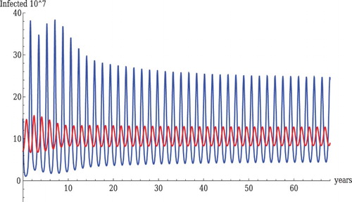
We investigate scenarios of coexistence of LPAI and HPAI in wild and domestic birds in the form of an equilibrium or in the form of sustained oscillations. We will call the order of prevalences ‘realistic’ if in the wild birds LPAI prevalence is higher than HPAI prevalence, and in domestic birds HPAI prevalence is higher than LPAI prevalence. We expect our prevalences in the simulations to be in this realistic order.

Figure shows a coexistence equilibrium with realistic parameter values and realistic prevalence order, that is HPAI prevalence in domestic birds is higher than that of LPAI and LPAI prevalence for wild birds is higher than that of HPAI. The solution stabilizes to an equilibrium. We note that in Figure at equilibrium $16.63$ domestic birds are HPAI infected out of a total of 826 domestic birds at equilibrium (both times $10^{7}$ ), giving as infection rate of 1 in 50. Just for a comparison, in a recent outbreak of HPAI in the US poultry industry approximately 50 million birds were affected out of 2 billion birds [Citation25] which is 1 in 40. Thus, our figure is a reasonable approximation of reality.

Figure 2. Coexistence with realistic parameter values. The parameter values used in the figure are as follows: $Λ_{w} = 2000$ , $μ_{w} = 0.25$ , $ν_{H_{w}} = 36.5$ , $α_{H_{w}} = 36.5$ , $α_{L_{w}} = 73$ , $q_{w} = 0.5$ , $β_{11}^{L} = .018776$ , $β_{11}^{H} = 0.005$ , $Λ_{d} = 1020$ , $μ_{d} = 0.5$ , $ν_{H_{d}} = 36.5$ , $α_{d} = 52.14$ , $q_{d} = 0.5$ , $β_{22}^{L} = .02539$ , $β_{22}^{H} = 0.04897$ , $β_{12}^{L} = 0.006$ , $β_{21}^{L} = 0.03$ , $β_{12}^{H} = 0.002$ , $β_{21}^{H} = 0.031$ . The reproduction numbers are $R_{L} = 2.54$ and $R_{H} = 2.71$ . The invasion coefficients are as follows: ${\hat{R}}_{L}^{H} = 1.75$ and ${\hat{R}}_{H}^{L} = 1.98$ . The red line shows HPAI in wild birds, the orange dashed line shows HPAI in domestic birds, the blue line shows LPAI in wild birds, the green dashed line shows LPAI in domestic birds.

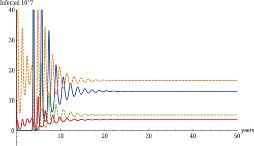
For Figure , the LPAI reproduction numbers are $R_{11}^{L} = 2.05$ , $R_{12}^{L} = 0.91$ , $R_{21}^{L} = 0.835$ , and $R_{22}^{L} = 0.984$ . In addition, the HPAI reproduction numbers are $R_{11}^{H} = 0.546$ , $R_{12}^{H} = 0.432$ , $R_{21}^{H} = 0.0863$ , and $R_{22}^{H} = 2.7$ . The invasion numbers are ${\hat{R}}_{L}^{H} = 1.75$ and ${\hat{R}}_{H}^{L} = 1.98$ . We see that, as we expect, the population-specific reproduction numbers of LPAI in wild birds and HPAI in domestic birds are higher than one; all other numbers are lower than one. With these parameters, wild birds are a sink for HPAI with realistic parameter values and a realistic order of prevalences. We note that we can obtain with realistic parameters and realistic prevalence order a case where HPAI in wild birds is a source. However, the $I_{H_{w}}$ would be larger and a larger $I_{H_{w}}$ should be more detectable in practice. Thus with the available information, we cannot deduce for sure whether HPAI will persist on its own in wild birds; however, the model suggests that the situation is closest to reality if HPAI is a sink for wild birds.

Figure shows that the full system can exhibit sustained, complex oscillations. We note that the prevalences are generally in realistic order and the parameters used in the examples are biologically reasonable. For wild birds, LPAI is generally higher than HPAI. The reversed order is observed for domestic birds. The oscillations of LPAI and HPAI are shifted half a period both in wild and domestic birds. That is, when LPAI is at high values, HPAI is at low values and vice versa. This is a manifestation of the competition of LPAI and HPAI for susceptible hosts in both wild and domestic birds. We note that in the full system oscillations can be obtained for relatively intermediate or low values for $q_{w}$ and $q_{d}$ , which shows that even intermediate levels of cross-immunity to HPAI can destabilize the system. The parameters $ν_{H_{d}}$ and $ν_{H_{w}}$ change the shape of the oscillations. In general, oscillations, whenever found, are observed in a moderate neighbourhood of the parameters for which they occur.

Figure 3. Oscillations with realistic parameter values. The parameter values used in the figure are as follows: $Λ_{w} = 2000$ , $μ_{w} = 0.25$ , $ν_{H_{w}} = 36.5$ , $α_{H_{w}} = 36.5$ , $α_{L_{w}} = 73$ , $q_{w} = 0.45$ , $β_{11}^{L} = .018776$ , $β_{11}^{H} = 0.015$ , $Λ_{d} = 1020$ , $μ_{d} = 0.5$ , $ν_{H_{d}} = 36.5$ , $α_{d} = 52.14$ , $q_{d} = 0.5$ , $β_{22}^{L} = .025$ , $β_{22}^{H} = 0.04897$ , $β_{12}^{L} = 0.006$ , $β_{21}^{L} = 0.03$ , $β_{12}^{H} = 0.0$ , $β_{21}^{H} = 0.031$ . The reproduction numbers are $R_{L} = 2.54$ and $R_{H} = 2.7$ . The invasion coefficients are as follows: ${\hat{R}}_{L} = 1.37$ and ${\hat{R}}_{H} = 1.86$ . The red line shows HPAI in wild birds, the orange dashed line shows HPAI in domestic birds, the blue line shows LPAI in wild birds, the green dashed line shows LPAI in domestic birds.

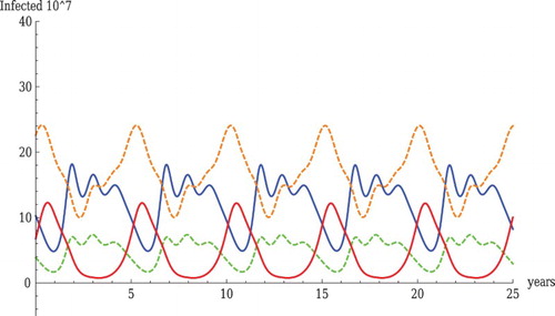
Furthermore, we note that oscillation and persistence of HPAI occurs in the case when $β_{12}^{H} = 0$ , that is when transmission from domestic to wild birds of HPAI does not occur. In this case, persistence of HPAI is only possible if $R_{11}^{H} > 1$ . We note that HPAI in wild birds emerges (or is likely detectable) only from time to time.

Figure is an illustration of a sink–sink scenario for both pathogens. A sink–sink scenario is a scenario where both pathogens are sinks for each of the populations but they can persist together in a coexistence equilibrium. We say that a sink–sink scenario occurs if the following is satisfied in each of the populations if they are isolated (no cross-transmission):

The reproduction numbers and the invasion numbers of both pathogens are smaller than one.

Figure 4. Coexistence with realistic parameter values. The parameter values used in the figure are as follows: $Λ_{w} = 2000$ , $μ_{w} = 0.25$ , $ν_{H_{w}} = 36.5$ , $α_{H_{w}} = 36.5$ , $α_{L_{w}} = 73$ , $q_{w} = 0.426$ , $β_{11}^{L} = .0086$ , $β_{11}^{H} = 0.005$ , $Λ_{d} = 1020$ , $μ_{d} = 0.5$ , $ν_{H_{d}} = 36.5$ , $α_{d} = 52.14$ , $q_{d} = 1$ , $β_{22}^{L} = .02539$ , $β_{22}^{H} = 0.0166$ , $β_{12}^{L} = 0.0043$ , $β_{21}^{L} = 0.0131$ , $β_{12}^{H} = 0.0014$ , $β_{21}^{H} = 0.0332$ . The reproduction numbers are $R_{L} = 1.45$ and $R_{H} = 1.29$ . The invasion coefficients are as follows: $\hat{R_{L}} = 1.17$ and $\hat{R_{H}} = 1.22$ . The red line shows HPAI in wild birds, the orange dashed line shows HPAI in domestic birds, the blue line shows LPAI in wild birds, the green dashed line shows LPAI in domestic birds.

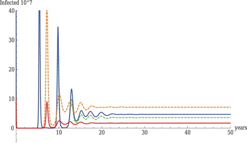
We were able to produce an example of this scenario, where all intra- and cross-population components of the reproduction numbers and invasion reproduction numbers are smaller than one. The coexistence of LPAI and HPAI under a sink–sink scenario is shown in Figure . All components of the reproduction numbers and the invasion reproduction numbers are smaller than one:

Table

Display Table

In this case, if all cross-coefficients $β_{12}^{p} = β_{21}^{p} = 0$ , where $p = L, H$ , then both LPAI and HPAI will die out. Persistence of both pathogens occurs only through the cross-population transmission. This scenario is easy to find with no constraints on parameters, but in our example, the parameters are plausible and we have a realistic prevalence order in wild and domestic birds.

4.4. LPAI and HPAI dynamics in the wild bird system only

We saw that the full ODE system corresponding to system (Equation1(1) $\begin{aligned} \frac{d S_{w}}{d t} & = Λ_{w} - λ_{L_{w}} S_{w} - λ_{H_{w}} S_{w} - μ_{w} S_{w}, \\ \frac{d I_{L_{w}}}{d t} & = λ_{L_{w}} S_{w} - (μ_{w} + α_{L_{w}}) I_{L_{w}}, \\ \frac{\partial r_{L_{w}}}{\partial t} + \frac{\partial r_{L_{w}}}{\partial τ} & = - q_{w} (τ) λ_{H_{w}} r_{L_{w}} - μ_{w} r_{L_{w}}, \\ r_{L_{w}} (0, t) & = α_{L_{w}} I_{L_{w}}, \\ \frac{d I_{H_{w}}}{d t} & = λ_{H_{w}} S_{w} + λ_{H_{w}} \int_{0}^{\infty} q_{w} (τ) r_{L_{w}} (τ, t) d τ - (μ_{w} + α_{H_{w}} + ν_{H_{w}}) I_{H_{w}}, \\ \frac{d R_{H_{w}}}{d t} & = α_{H_{w}} I_{H_{w}} - μ_{w} R_{H_{w}}, \\ \frac{d S_{d}}{d t} & = Λ_{d} - λ_{L_{d}} S_{d} - λ_{H_{d}} S_{d} - μ_{d} S_{d}, \\ \frac{d I_{L_{d}}}{d t} & = λ_{L_{d}} S_{d} - (μ_{d} + α_{d}) I_{L_{d}}, \\ \frac{\partial r_{d}}{\partial t} + \frac{\partial r_{d}}{\partial τ} & = - q_{d} (τ) λ_{H_{d}} r_{d} - μ_{d} r_{d}, \\ r_{d} (0, t) & = α_{d} I_{L_{d}}, \\ \frac{d I_{H_{d}}}{d t} & = λ_{H_{d}} S_{d} + λ_{H_{d}} \int_{0}^{\infty} q_{d} (τ) r_{d} (τ, t) d τ - (μ_{d} + ν_{H_{d}}) I_{H_{d}} . \end{aligned}$ (1) ) can exhibit oscillations where LPAI and HPAI coexist. An interesting question occurs whether the coexistence equilibrium can lose stability if restricted to just the wild bird system. This question is of particular importance in the ODE case as it is well known that alternative ODE models with cross-immunity do not always lead to oscillations. For instance, Castillo-Chavez et al. found that age structure or quarantine needs to be introduced for a cross-immunity model to show oscillations [Citation3, Citation4]. However, it turns out that this is not the case with system (Equation1(1) $\begin{aligned} \frac{d S_{w}}{d t} & = Λ_{w} - λ_{L_{w}} S_{w} - λ_{H_{w}} S_{w} - μ_{w} S_{w}, \\ \frac{d I_{L_{w}}}{d t} & = λ_{L_{w}} S_{w} - (μ_{w} + α_{L_{w}}) I_{L_{w}}, \\ \frac{\partial r_{L_{w}}}{\partial t} + \frac{\partial r_{L_{w}}}{\partial τ} & = - q_{w} (τ) λ_{H_{w}} r_{L_{w}} - μ_{w} r_{L_{w}}, \\ r_{L_{w}} (0, t) & = α_{L_{w}} I_{L_{w}}, \\ \frac{d I_{H_{w}}}{d t} & = λ_{H_{w}} S_{w} + λ_{H_{w}} \int_{0}^{\infty} q_{w} (τ) r_{L_{w}} (τ, t) d τ - (μ_{w} + α_{H_{w}} + ν_{H_{w}}) I_{H_{w}}, \\ \frac{d R_{H_{w}}}{d t} & = α_{H_{w}} I_{H_{w}} - μ_{w} R_{H_{w}}, \\ \frac{d S_{d}}{d t} & = Λ_{d} - λ_{L_{d}} S_{d} - λ_{H_{d}} S_{d} - μ_{d} S_{d}, \\ \frac{d I_{L_{d}}}{d t} & = λ_{L_{d}} S_{d} - (μ_{d} + α_{d}) I_{L_{d}}, \\ \frac{\partial r_{d}}{\partial t} + \frac{\partial r_{d}}{\partial τ} & = - q_{d} (τ) λ_{H_{d}} r_{d} - μ_{d} r_{d}, \\ r_{d} (0, t) & = α_{d} I_{L_{d}}, \\ \frac{d I_{H_{d}}}{d t} & = λ_{H_{d}} S_{d} + λ_{H_{d}} \int_{0}^{\infty} q_{d} (τ) r_{d} (τ, t) d τ - (μ_{d} + ν_{H_{d}}) I_{H_{d}} . 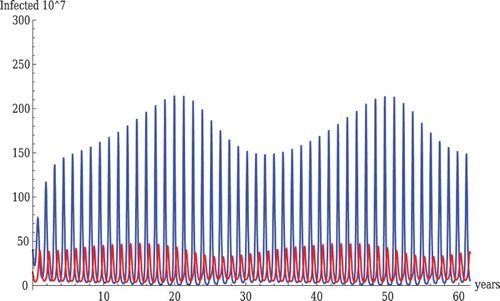\end{aligned}$ (1) ) with wild birds only. The characteristic equation of the coexistence equilibrium looks ‘almost’ stable but for some parameter values the coexistence equilibrium can be destabilized (the analytical expression giving parameter combinations for which the system is unstable is too complicated to interpret, so we illustrate instability with numerical examples). Figure shows sustained oscillations for both LPAI and HPAI. The oscillations in LPAI have much larger amplitude. HPAI peaks follow LPAI peaks by about 1/4 period which is typical for classical predator–prey dynamics. The parameters chosen including the reproduction numbers and invasion reproduction numbers have plausible values. To obtain oscillations with these parameter choices, our simulations suggested that we need to choose $q_{w} \approx 1$ . That suggests that oscillations, which often mimic outbreaks, occur if the LPAI cross-immunity to HPAI is nearly or completely non-existent. Figure also shows sustained oscillations. Looking more closely at the figure, we can see two oscillation patterns superimposed, differing in period. With the short period oscillations, the peak of LPAI is followed by a peak of HPAI, somewhat resembling predator–prey oscillations. The unstable equilibrium values are given by $(S_{w}, I_{L_{w}}, R_{L_{w}}, I_{H_{w}}, R_{H_{w}}) = (5301.83, 38.2707, 12316.7, 16.3273, 26426.1)$ . In the simulation in Figure , the reproduction number of LPAI is somewhat high to be realistic. Decreasing $q_{w}$ to $0.9$ from the parameter listed in Figure allows the oscillations of LPAI and HPAI to be shifted so they are half the period out of phase, so that the maximum of HPAI occurs at the same moment as the minimum of LPAI. In this case, we say the the system exhibits fully competitive oscillation.

Figure 5. Sustained oscillations in the wild birds only system. Parameter values are $Λ_{w} = 2000$ , $μ_{w} = 0.14$ , $ν_{H_{w}} = 49.5$ , $α_{H_{w}} = 51.6$ , $α_{L_{w}} = 73$ , $q_{w} = 0.98$ , $β_{11}^{L} = .018776$ , $β_{11}^{H} = 0.015$ , $S_{w} (0) = 3449.72$ , $I_{L_{w}} (0) = 14.684$ , $R_{L_{w}} (0) = 3366.78$ , $I_{H_{w}} (0) = 7$ , $R_{H_{w}} (0) = 769.5$ . The reproduction numbers are $R_{L} = 3.66$ and $R_{H} = 2.116$ . The invasion coefficients are ${\hat{R}}_{L} = 1.73$ and ${\hat{R}}_{H} = 2.08$ . The red line shows HPAI and the blue line shows LPAI.

It is useful to develop some intuitive understanding for why oscillations arise in this system. Biologically, the system is not really analogous to a predator–prey system. Recall that LPAI and HPAI both attack susceptible hosts. If $q_{w} = 0$ , there is complete cross-immunity, and the relation between LPAI and HPAI is simply that of being competitors for susceptible hosts. One does not find coexistence in this case in a single population. In this model, infection by HPAI always gives complete immunity to LPAI. However, if $q_{w} > 0$ , there is only partial (or no) immunity to HPAI conferred by prior infection by LPAI, so LPAI-recovered hosts can be infected by HPAI. A direct predation analogue in this system would be if HPAI could infect LPAI-infected hosts and eliminate the LPAI infection, thereby directly reducing the number of LPAI-infected hosts. In our model, HPAI does not have this direct effect because it just attacks LPAI-recovered hosts. However, attacking LPAI-recovered hosts increases the prevalence of HPAI, and allows it to infect more susceptible hosts, for which it is competing with LPAI. It would, therefore, be analogous to a system in which one competitor can consume the carcasses of the other. For the parameters of Figure , the number of LPAI-infected hosts increases whenever $S_{w} > (μ_{w} + α_{L_{w}}) / β_{ww}^{L} = 5302$ and decreases otherwise. As $I_{L_{w}}$ increases, it decreases $S_{w}$ until it is below this value (HPAI also helps decrease $S_{w}$ , but it is less common, especially when $I_{L_{w}}$ is near its peak). For HPAI to increase requires $S_{w} + q_{w} R_{L_{w}} > (μ_{w} + α_{H_{w}} + ν_{H_{w}}) / β_{ww}^{H} = 17, 495.$ Even though this threshold is higher (due to the high death rate), it applies to the sum of susceptible and LPAI-recovered hosts (the latter discounted by $q_{w}$ ). Because most LPAI-infected birds recover, as the peak in $I_{L_{w}}$ draws down $S_{w}$ , it also increases $R_{L_{w}}$ , so that the condition for HPAI to increase can sometimes continue to be met after LPAI has started to decrease, as in the figure. For the parameters of the figure, HPAI relies mostly on LPAI-recovered birds, the peak of which is after the peak in $I_{L_{w}}$ . HPAI, therefore, is increasing most rapidly after the LPAI peak. Eventually, HPAI depletes the hosts it attacks, and starts to decrease. By this time, the susceptible hosts have started to increase (because of the low level of $I_{L_{w}}$ ), but they then increase faster until they are high enough for $I_{L_{w}}$ to start to increase. So oscillations in this system arise because of a combination of competition, and a phenomenon analogous to ‘scavenging’ among carnivores.

Figure 6. Sustained oscillations in the wild birds only system. Parameter values are $Λ_{w} = 3810$ , $μ_{w} = 0.054$ , $ν_{H_{w}} = 87.5$ , $α_{H_{w}} = 87.4$ , $α_{L_{w}} = 69.4$ , $q_{w} = 0.99$ , $β_{11}^{L} = .0131$ , $β_{11}^{H} = 0.01$ , $S_{w} (0) = 5000$ , $I_{L_{w}} (0) = 40$ , $R_{L_{w}} (0) = 12000$ , $I_{H_{w}} (0) = 15$ , $R_{H_{w}} (0) = 25, 000$ . The reproduction numbers are $R_{L} = 13.3$ and $R_{H} = 4.0$ . The invasion coefficients are ${\hat{R}}_{L} = 3.3$ and ${\hat{R}}_{H} = 4$ . The red line shows HPAI and the blue line shows LPAI.

We next address the question of whether we can reduce $q_{w}$ and still obtain oscillations. The most influential parameter for that to occur is $μ_{w}$ , which needs to be fairly low ( $0.14$ in Figure and $0.054$ in Figure , both reasonable for wild birds) to produce oscillations with smaller $q_{w}$ . Raising $Λ_{w}$ allows oscillations without $μ_{w}$ becoming excessively small and therefore unrealistic for wild bird populations. Raising the sum $α_{H_{w}} + ν_{H_{w}}$ also allows for lowering $q_{w}$ . Still with nearly realistic other parameters, $q_{w}$ needs to stay above $0.9$ for oscillations to occur.

LPAI persists at higher levels than HPAI in Figures –, which is the realistic scenario for wild bird populations. However, raising $q_{w}$ as in Figures and leads to oscillations but also increases the prevalence of HPAI at times to levels higher than LPAI which in wild birds is unrealistic. Lack of cross-immunity from LPAI in domestic birds may explain why HPAI persists in domestic birds at higher prevalence levels.

For realistic parameter values, it appears that in most cases oscillations of LPAI have larger amplitude and go to higher values compared to oscillations in HPAI. In the future, we expect that long-term empirical time-series of AI will become available. There is considerable temporal variability in avian flu prevalence, and the processes we have explored could help explain some of the drivers of these dynamics. Our model predictions about phase shifts and differences in amplitude for flu strains differing in pathogenicity and cross-infectivity should be useful in future studies in interpreting patterns in such data.

5. Discussion

AI continues to be a threat to human health. Recently, strains of HPAI H7N9 have started infecting humans and hold potential to turn pandemic with deadly consequences. Studying AI in birds and humans is of paramount importance if we are to be prepared for the next deadly pandemic.

In this paper, we introduce an AI model for multiple bird populations. The model incorporates two strains, one LPAI and one HPAI. We are interested in studying the dynamics of LPAI and HPAI in wild and domestic birds. Our model builds on previous work. Several models published before have studied the interplay between LPAI and HPAI. Lucchetti et al. [Citation13] were the first to introduce LPAI and HPAI but the wild bird population in that article is taken as a periodic source, not as a dynamical variable. Bourouiba et al. [Citation2] studied the transmission of LPAI and HPAI in wild bird populations only. They assumed no cross-immunity and that LPAI-recovered birds can get infected by HPAI with the same transmission coefficients as do susceptible birds. However, reinfected wild birds can show higher survivability. The results of this article are mostly obtained through simulations and are specific to the parameters chosen. A model close to the one considered here is introduced by Augusto and Gumel [Citation1]. This model studies LPAI and HPAI in both wild and domestic birds and assumes reinfection by HPAI of exposed and infectious birds with LPAI. It assumes that the partial immunity to HPAI conferred by LPAI infection is fixed, whereas we allow it to wane with time (so their model is a pure ODE model, whereas ours includes PDEs). Also, their model includes exposed (infectious but asymptomatic) classes, and includes two mechanisms by which LPAI can change into HPAI. One is mutation, which takes place in LPAI-exposed birds but produces HPAI-exposed and HPAI-infected birds. In the other process, when LPAI-exposed birds become symptomatic (enter an infected class), a fraction of them become LPAI-infected and the rest become HPAI-infected birds. (In addition, birds with LPAI can become infected by HPAI, as in our model.) This article finds backward bifurcation and multiple coexistence equilibria which are caused by the reinfection with HPAI of LPAI-exposed birds and LPAI-infected birds. The article makes two conjectures which are both true and are explained in the case of wild birds only in [Citation23]. One of our main contributions here relative to article [Citation1] is that we provide rigorous analytical results for when each strain persists and when it dies out, and when the two strains coexist for the case when both reproduction numbers are greater than one. These are quantified in terms of the invasion reproduction numbers and are satisfied for all parameter values. One difference from the model in [Citation1] is that our model does not exhibit backward bifurcation. Also, of course, we allow cross-immunity to fade with time.

We compute the reproduction numbers $R_{L}$ and $R_{H}$ and the invasion reproduction numbers ${\hat{R}}_{L}^{H}$ and ${\hat{R}}_{H}^{L}$ . The model has a unique DFE which is locally and globally stable if both reproduction numbers are smaller than one. The global stability of the DFE rules out backward bifurcation. There are also a unique LPAI-only and a unique HPAI-only equilibria which exist if the LPAI (HPAI) reproduction number is larger than one. The LPAI-only equilibrium is locally asymptotically stable whenever it exists if ${\hat{R}}_{L}^{H} < 1$ . The HPAI-only equilibrium is locally asymptotically stable whenever it exists if ${\hat{R}}_{H}^{L} < 1$ . We show that if ${\hat{R}}_{H}^{L} > 1$ and ${\hat{R}}_{L}^{H} > 1$ , then a coexistence equilibrium exists. The question about the uniqueness of the coexistence equilibrium remains open.

Simulations suggest that the coexistence equilibrium is not stable for all parameter regimes. In fact, the coexistence equilibrium can be destabilized even in the corresponding ODE system in which $q_{w}$ and $q_{d}$ are assumed constant. Since the semi-trivial equilibria are locally stable, this clearly suggests that the interaction between the strains, that is $q_{w} \neq 0$ and/or $q_{d} \neq 0$ , is necessary for the destabilization of the coexistence equilibrium. Next, we asked whether the presence of both populations and transmission between the populations were necessary for instability. Investigating the wild bird system only [Citation22], we find numerically that the ODE model of wild birds with LPAI and HPAI also can exhibit oscillations in which both LPAI and HPAI persist. In the wild bird system, oscillations are found with high values of $q_{w} \approx 1$ , which means that destabilization of the system occurs if cross-immunity is very low. In the full system, oscillations can be found for larger ranges of $q_{w}$ and $q_{d}$ . Thus, transmission between the two populations allows for destabilization of the system for a variety of cross-immunity levels. For sustained oscillations in a single population considered alone, LPAI-recovered birds must be almost as susceptible to HPAI infection as are naive birds.

Simulations suggest that for plausible parameter values, we can also produce realistic prevalences. In particular, in wild birds, the LPAI prevalence is higher than the HPAI prevalence, while in domestic birds, it is vice versa. Of particular interest is the case when a population is a sink for a pathogen but persistence in a multi-population multi-pathogen system is still possible. We call population A a sink for pathogen p, where $p =$ LPAI or HPAI, if pathogen p cannot persist alone in population A, if isolated. It is well known that, in a system with two sink habitats, a population can sometimes persist by using both habitats. We have investigated this question in the case of competition of pathogens. In the case of competition, we say that a population A is a sink for pathogen p if its within-population reproduction number is less than one, or if its reproduction number is greater than one, its within-population invasion reproduction number is smaller than one and the other pathogen is present. We show through simulations that coexistence of both pathogens is possible, if all their within-population and cross-population reproduction numbers are smaller than one. This observation is very important since estimates of the reproduction number of HPAI H5N1 in poultry vary around one [Citation14, Citation15, Citation24] but our results imply that even if the reproduction number is below one, HPAI may persist in the wild-domestic bird system, even under competition with LPAI. We note that in the sink–sink scenario, even though the species-specific, strain-specific reproduction and invasion numbers are below one, the overall strain-specific reproduction and invasion numbers are above one, which gives persistence.

Future empirical studies will be required to refine parameter estimation and ascertain the likelihood of observing the complex dynamics revealed by this model. Also, in the future it would be useful to explore alternative models of recruitment instead of the constant rate of input assumed in model (Equation1(1) $\begin{aligned} \frac{d S_{w}}{d t} & = Λ_{w} - λ_{L_{w}} S_{w} - λ_{H_{w}} S_{w} - μ_{w} S_{w}, \\ \frac{d I_{L_{w}}}{d t} & = λ_{L_{w}} S_{w} - (μ_{w} + α_{L_{w}}) I_{L_{w}}, \\ \frac{\partial r_{L_{w}}}{\partial t} + \frac{\partial r_{L_{w}}}{\partial τ} & = - q_{w} (τ) λ_{H_{w}} r_{L_{w}} - μ_{w} r_{L_{w}}, \\ r_{L_{w}} (0, t) & = α_{L_{w}} I_{L_{w}}, \\ \frac{d I_{H_{w}}}{d t} & = λ_{H_{w}} S_{w} + λ_{H_{w}} \int_{0}^{\infty} q_{w} (τ) r_{L_{w}} (τ, t) d τ - (μ_{w} + α_{H_{w}} + ν_{H_{w}}) I_{H_{w}}, \\ \frac{d R_{H_{w}}}{d t} & = α_{H_{w}} I_{H_{w}} - μ_{w} R_{H_{w}}, \\ \frac{d S_{d}}{d t} & = Λ_{d} - λ_{L_{d}} S_{d} - λ_{H_{d}} S_{d} - μ_{d} S_{d}, \\ \frac{d I_{L_{d}}}{d t} & = λ_{L_{d}} S_{d} - (μ_{d} + α_{d}) I_{L_{d}}, \\ \frac{\partial r_{d}}{\partial t} + \frac{\partial r_{d}}{\partial τ} & = - q_{d} (τ) λ_{H_{d}} r_{d} - μ_{d} r_{d}, \\ r_{d} (0, t) & = α_{d} I_{L_{d}}, \\ \frac{d I_{H_{d}}}{d t} & = λ_{H_{d}} S_{d} + λ_{H_{d}} \int_{0}^{\infty} q_{d} (τ) r_{d} (τ, t) d τ - (μ_{d} + ν_{H_{d}}) I_{H_{d}} . \end{aligned}$ (1) ). Finally, it is likely that spatial dynamics are significant in this system. Many wild waterfowl are migratory and can move over large areas. Some birds may return to the same area each winter, but others may move among regions. Domestic fowl are concentrated in more discrete locations, with less mobility, one expects. Dealing with spatial patchiness, migration and heterogeneity will likely be important in more realistic future characterizations of cross-population transmission in AI.

Acknowledgments

RDH and MB thank the University of Florida Foundation for support.

Disclosure statement

No potential conflict of interest was reported by the authors.

ORCID

Necibe Tuncer http://orcid.org/0000-0002-6388-2499

Additional information

Funding

This work was supported by the US National Science Foundation [grant number DMS 1220342].

References

F.B. Agusto and A.B. Gumel, Qualitative dynamics of lowly and highly-pathogenic avian influenza strains, Math. Biosci. 243 (2013), pp. 147–162. doi: 10.1016/j.mbs.2013.02.001
Google Scholar
L. Bourouiba, A. Teslya, and J. Wu, Highly pathogenic avian influenza outbreak mitigated by seasonal low pathogenic strains: Insights from dynamic modeling, JTB 271 (2011), pp. 181–201. doi: 10.1016/j.jtbi.2010.11.013
Google Scholar
C. Castillo-Chavez, H. Hethcote, V. Andreasen, S. Levin, and W.M. Liu, Epidemiological models with age structure, proportionate mixing and cross-immunity, J. Math. Biol. 27 (1989), pp. 159–165.
Google Scholar
C. Castillo-Chavez, H. Hethcote, V. Andreasen, S. Levin, and W.M. Liu, Cross-immunity in the dynamics of homogeneous and heterogeneous populations, Mathematical Ecology (Trieste, 1986), World Sci. Publishing, Teaneck, NJ, 1988, pp. 303–316.
Google Scholar
J.J. Dennehy, N. A. Friedenberg, R. C. McBride, R. D. Holt, and P. E. Turner, Experimental evidence that source genetic variation drives pathogen emergence, Proc. R. Soc. Lond. Ser. B 277(1697) (2010), pp. 3113–3121. doi: 10.1098/rspb.2010.0342
Google Scholar
P. van den Driessche and J. Watmough, Reproduction numbers and sub-threshold endemic equilibria for compartmental models of disease transmission, Math. Biosci. 180 (2002), pp. 29–48. doi: 10.1016/S0025-5564(02)00108-6
Google Scholar
A. Dobson, Population dynamics of pathogens with multiple host species, Amer. Natural. 164 (2004), pp. 564–576. doi: 10.1086/424681
Google Scholar
E. O'Neill, J.M. Riberdy, R.G. Webster, and D.L. Woodland, Heterologous protection against lethal A/Hong Kong/156/97 (H5N1) influenza virus infection in C57BL/6 mice, J. Gen. Virol. 81 (2000), pp. 2689–2696. doi: 10.1099/0022-1317-81-11-2689
Google Scholar
R.D. Holt and A.P. Dobson, Extending the principles of community ecology to address the epidemiology of host-pathogen systems, in Ecology of Emerging Infectious Diseases, S.K. Collinge and C. Ray, eds., OUP, Oxford, 2005, pp. 6–27.
Google Scholar
M.J. Keeling and P. Rohani, Modeling Infectious Diseases in Humans and in Animals, Princeton University Press, Princeton, 2008.
Google Scholar
T. Kuiken, Is low pathogenic avian influenza virus virulent for wild waterbirds? Proc. Biol. Sci. 280(1763) (2013), 20130990. doi: 10.1098/rspb.2013.0990. doi: 10.1098/rspb.2013.0990
Google Scholar
N. Latorre-Margalef, C. Tolf, V. Grosbois, A. Avril, D. Bengtsson, M. Wille, A. D. M. E. Osterhaus, R. A. M. Fouchier, B. Olsen, and J. Waldenstrom, Long-term variation in influenza A virus prevalence and subtype diversity in migratory mallards in northern Europe, Proc. R. Soc. B 281 (2014), pp. 20140098. doi: 10.1098/rspb.2014.0098
Google Scholar
J. Lucchetti, M. Roy, and M. Martcheva, An avian influenza model and its fit to human avian influenza cases, in Advances in Disease Epidemiology, J.M.Tchuenche and Z. Mukandavire, eds., Nova Science Publishers, New York, NY, 2009, pp. 1–30.
Google Scholar
M. Martcheva, Avian influenza: Modeling and implications for control, Math. Mod. Nat. Phenom. (to appear).
Google Scholar
P.S. Pandit, D.A. Bunn, S.A. Pande, and S.S. Aly, Modeling highly pathogenic avian influenza transmission in wild birds and poultry in West Bengal, India, Sci. Rep. 3 (2013), article number 2175, pp. 1–8. doi: 10.1038/srep02175
Google Scholar
K.M. Pepin, E. Spackman, J.D. Brown, K.L. Pabilonia, L.P. Garber, J.T. Weaver, D.A. Kennedy, K.A. Patyk, K.P. Huyvaert, R.S. Miller, A.B. Franklin, K. Pedersen, T.L. Bogich, P. Rohani, S.A. Shriner, C.T. Webb, and S. Riley, Using quantitative disease dynamics as a tool for guiding response to avian influenza in poultry in the United States of America, Prevent. Veterinary Med. 113 (2014), pp. 376–397. doi: 10.1016/j.prevetmed.2013.11.011
Google Scholar
I. Scones and P. Forster, Unpacking the International Response to Avian Influenza: Actors, Networks and Narratives, in Avian Influenza: Science, Policy and Politics, I. Scoones, ed., EarthScan, London, 2010, pp. 19–64.
Google Scholar
S.H. Seo and R.G. Webster, Cross-reactive, cell-mediated immunity and protection of chickens from lethal H5N1 influenza virus infection in Hong Kong poultry markets, J. Virol. 75 (2001), pp. 2516–2525. doi: 10.1128/JVI.75.6.2516-2525.2001
Google Scholar
E. Spackman, A brief introduction to the avian influenza virus, in Avian Influenza Virus, E. Spackman, ed., Humana Press, Totowa, NJ, 2008, pp. 1–6.
Google Scholar
D.L. Suarez, Influenza A Virus, in Avian Influenza, D.E. Swayne, ed., Blackwell Publishing, Ames, IA, 2008, pp. 3–17.
Google Scholar
J. Takekawa, D. Prosser, B. Collins, D. Douglas, W. Perry, B. Yan, L. Ze, Y. Hou, F. Lei, T. Li, Y. Li, and S. Newman, Movements of wild Ruddy Shelducks in the Central Asian Flyway and their spatial relationship to outbreaks of highly pathogenic avian influenza H5N1, Viruses 5 (2013), pp. 2129–2152. doi: 10.3390/v5092129
Google Scholar
N. Tuncer, J. Torres, and M. Martcheva, Dynamics of low and high pathogenic avian influenza in wild bird population, in Dynamical Systems: Theory, Applications and Future Directions, J. Thuenche, ed., Nova Publishers, New York, 2013, pp. 235–259.
Google Scholar
N. Tuncer, J. Torres, and M. Martcheva, Dynamics of low and high pathogenic avian influenza in birds, Biomath. Commun. 1(1) (2014), pp. 5–11.
Google Scholar
N. Tuncer and M. Martcheva, Modeling seasonality in avian influenza H5N1, J. Biol. Syst. 21(4) (2013), pp. 1450009. doi: 10.1142/S0218339013400044
Google Scholar
USDA, Animal and Plant Health Inspection Service. Available at http://www.aphis.usda.gov/wps/portal/aphis/ourfocus/animalhealth/sa_animal_disease_information/sa_avian_health/ct_avian_influenza_disease/.
Google Scholar
R.G. Webster, W.J. Bean, O.T. Gorman, T.M. Chambers, and Y. Kawaoka, Evolution and ecology of influenza A viruses, Microbiol. Rev. 56(1) (1992), pp. 152–179.
Google Scholar

Appendix 1. LPAI-only equilibrium

Proposition A.1. Let

D P (u)

denote the derivative of the operator P; then, the spectral radius of

D P (u)

is less than 1.

Proof.

The derivative of the operator P is $D P (u) = (\begin{matrix} κ_{1} \frac{μ_{w}}{(u_{1} + μ_{w})^{2}} & κ_{2} \frac{μ_{d}}{(u_{2} + μ_{d})^{2}} \\ κ_{3} \frac{μ_{w}}{(u_{1} + μ_{w})^{2}} & κ_{4} \frac{μ_{d}}{(u_{2} + μ_{d})^{2}} \end{matrix})$ . Note that $D P (u)$ is a positive matrix, since all its entries are positive. Let A be a $2 \times 2$ square matrix given as $A = (\begin{matrix} \frac{κ_{1}}{(u_{1} + μ_{w})} & \frac{κ_{2}}{(u_{2} + μ_{d})} \\ \frac{κ_{3}}{(u_{1} + μ_{w})} & \frac{κ_{4}}{(u_{2} + μ_{d})} \end{matrix}) .$ Clearly, $D P (u) \leq A$ . Since $P (u_{1}, u_{2}) = (u_{1}, u_{2})$ , dividing by $u_{1}$ we obtain $1 = \frac{κ_{1}}{u_{1} + μ_{w}} + \frac{κ_{2}}{u_{2} + μ_{d}} z, \frac{u_{2}}{u_{1}} = \frac{κ_{3}}{u_{1} + μ_{w}} + \frac{κ_{4}}{u_{2} + μ_{d}} z,$ where $z = \frac{u_{2}}{u_{1}} .$ Let $v = (\begin{matrix} 1 \\ z \end{matrix})$ , then $A v = v$ . Thus, 1 is an eigenvalue of A corresponding to a positive eigenvector. By Perron–Frobenius theorem, the spectral radius of A is $ρ (A) = 1$ . Furthermore, $ρ (D P (u)) < ρ (A)$ since $D P (u) < A$ .

Appendix 2. Coexistence equilibrium

Proposition A.2.

Derivatives of the nonlinear operator T satisfy the following inequalities: $\begin{aligned} \frac{\partial T_{i}}{\partial λ_{L_{w}}^{* *}} & > 0 \frac{\partial T_{i}}{\partial λ_{L_{d}}^{* *}} > 0 \frac{\partial T_{i}}{\partial λ_{H_{w}}^{* *}} < 0 \frac{\partial T_{i}}{\partial λ_{H_{d}}^{* *}} < 0 i = 1, 2, \\ \frac{\partial T_{i}}{\partial λ_{L_{w}}^{* *}} & < 0 \frac{\partial T_{i}}{\partial λ_{L_{d}}^{* *}} < 0 \frac{\partial T_{i}}{\partial λ_{H_{w}}^{* *}} > 0 \frac{\partial T_{i}}{\partial λ_{H_{d}}^{* *}} > 0 i = 3, 4. \end{aligned}$
T is monotone in $K_{T}$ , that is $u^{1} \leq_{K} u^{2} ⟹ T (u^{1}) \leq_{K} T (u^{2}) .$
T maps the set $C_{T}$ into itself. $T : C_{T} \to C_{T}$ .

Proof.

We only prove the inequalities $\partial T_{1} / \partial λ_{L_{w}}^{* *} > 0$ and $\partial T_{1} / \partial λ_{H_{w}}^{* *} < 0$ , since the inequalities of other derivatives when $i = 1, 2$ can be derived by applying the same steps. Note that $T_{1} (λ_{L_{w}}^{* *}, λ_{L_{d}}^{* *}, λ_{H_{w}}^{* *}, λ_{H_{d}}^{* *}) = \frac{Λ_{d} β_{12}^{L} λ_{L_{d}}^{* *}}{(α_{d} + μ_{d}) (μ_{d} + λ_{H_{d}}^{* *} + λ_{L_{d}}^{* *})} + \frac{Λ_{w} β_{11}^{L} λ_{L_{w}}^{* *}}{(α_{L_{w}} + μ_{w}) (μ_{w} + λ_{H_{w}}^{* *} + λ_{L_{w}}^{* *})} .$ Thus, $\begin{aligned} \frac{\partial T_{1}}{\partial λ_{L_{w}}^{* *}} & = \frac{(Λ_{w} β_{11}^{L}) (μ_{w} + λ_{H_{w}}^{* *})}{(α_{L_{w}} + μ_{w}) (μ_{w} + λ_{H_{w}}^{* *} + λ_{L_{w}}^{* *})^{2}} > 0 and \frac{\partial T_{1}}{\partial λ_{H_{w}}^{* *}} \\ = \frac{- Λ_{w} β_{11}^{L} λ_{L_{w}}^{* *}}{(α_{L_{w}} + μ_{w}) (μ_{w} + λ_{H_{w}}^{* *} + λ_{L_{w}}^{* *})^{2}} < 0. \end{aligned}$ Next, we prove the inequalities $\partial T_{3} / \partial λ_{L_{w}}^{* *} < 0$ and $\partial T_{3} / \partial λ_{H_{w}}^{* *} > 0.$ Inequalities for the other derivatives when $i = 3, 4$ can be shown in a similar way. Note that $T_{3} (λ_{L_{w}}^{* *}, λ_{L_{d}}^{* *}, λ_{H_{w}}^{* *}, λ_{H_{d}}^{* *}) = λ_{H_{w}}^{* *}$ as in Equation (Equation21(21) $\begin{aligned} λ_{H_{w}}^{* *} & = \frac{Λ_{w} β_{11}^{H} λ_{H_{w}}^{* *}}{(μ_{w} + α_{H_{w}} + ν_{H_{w}}) (μ_{w} + λ_{H_{w}}^{* *} + λ_{L_{w}}^{* *})} (1 + \frac{α_{L_{w}} λ_{L_{w}}^{* *}}{μ_{w} + α_{L_{w}}} \int_{0}^{\infty} q_{w} (τ) Π_{w} (τ) d τ) \\ + \frac{Λ_{d} β_{12}^{H} λ_{H_{d}}^{* *}}{(μ_{d} + ν_{H_{d}}) (μ_{d} + λ_{H_{d}}^{* *} + λ_{L_{d}}^{* *})} (1 + \frac{α_{d} λ_{L_{d}}^{* *}}{μ_{d} + α_{d}} \int_{0}^{\infty} q_{d} (τ) Π_{d} (τ) d τ), \end{aligned}$ (21) ). The derivative of $T_{3}$ with respect to $λ_{L_{w}}^{* *}$ is $\begin{aligned} \frac{\partial T_{3}}{\partial λ_{L_{w}}^{* *}} & = \frac{- Λ_{w} β_{11}^{H} λ_{H_{w}}^{* *}}{(μ_{w} + α_{H_{w}} + ν_{H_{w}}) (μ_{w} + λ_{H_{w}}^{* *} + λ_{L_{w}}^{* *})^{2}} (1 + \frac{α_{L_{w}} λ_{L_{w}}^{* *}}{μ_{w} + α_{L_{w}}} \int_{0}^{\infty} q_{w} (τ) Π_{w} (τ) d τ) \\ + \frac{Λ_{w} β_{11}^{H} λ_{H_{w}}^{* *}}{(μ_{w} + α_{H_{w}} + ν_{H_{w}}) (μ_{w} + λ_{H_{w}}^{* *} + λ_{L_{w}}^{* *})} (\frac{α_{L_{w}}}{μ_{w} + α_{L_{w}}} \int_{0}^{\infty} q_{w} (τ) Π_{w} (τ) d τ) . \end{aligned}$ Combining the terms, we obtain $\begin{aligned} \frac{\partial T_{3}}{\partial λ_{L_{w}}^{* *}} & = \frac{- Λ_{w} β_{11}^{H} λ_{H_{w}}^{* *}}{(μ_{w} + α_{H_{w}} + ν_{H_{w}}) (μ_{w} + λ_{H_{w}}^{* *} + λ_{L_{w}}^{* *})^{2}} \\ (1 - \frac{α_{L_{w}} (μ_{w} + λ_{H_{w}}^{* *})}{μ_{w} + α_{L_{w}}} \int_{0}^{\infty} q_{w} (τ) Π_{w} (τ) d τ) . \end{aligned}$ Clearly, $\partial T_{3} / \partial λ_{L_{w}}^{* *} < 0$ is negative, provided that (A1) $(μ_{w} + λ_{H_{w}}^{* *}) \int_{0}^{\infty} q_{w} (τ) Π_{w} (τ) d τ < 1.$ (A1) Since $0 \leq q_{w} (τ) \leq 1,$ the left side of Equation (EquationA1(A1) $(μ_{w} + λ_{H_{w}}^{* *}) \int_{0}^{\infty} q_{w} (τ) Π_{w} (τ) d τ < 1.$ (A1) ) is less than the following integral $\int_{0}^{\infty} (λ_{H_{w}}^{* *} q_{w} (τ) + μ_{w}) Π_{w} (τ) d τ = 1 (note that \int_{0}^{\infty} q_{w} (s) d s = \infty) .$ The derivative of $T_{3}$ with respect to $λ_{H_{w}}^{* *}$ is $\begin{aligned} \frac{\partial T_{3}}{\partial λ_{H_{w}}^{* *}} & = \frac{Λ_{w} β_{11}^{H} (μ_{w} + λ_{L_{w}}^{* *})}{(μ_{w} + α_{H_{w}} + ν_{H_{w}}) (μ_{w} + λ_{H_{w}}^{* *} + λ_{L_{w}}^{* *})^{2}} (1 + \frac{α_{L_{w}} λ_{L_{w}}^{* *}}{μ_{w} + α_{L_{w}}} \int_{0}^{\infty} q_{w} (τ) Π_{w} (τ) d τ) \\ - \frac{Λ_{w} β_{11}^{H} λ_{H_{w}}^{* *}}{(μ_{w} + α_{H_{w}} + ν_{H_{w}}) (μ_{w} + λ_{H_{w}}^{* *} + λ_{L_{w}}^{* *})} \\ (\frac{α_{L_{w}} λ_{L_{w}}^{* *}}{μ_{w} + α_{L_{w}}} \int_{0}^{\infty} q_{w} (τ) \int_{0}^{τ} q_{w} (s) d s Π_{w} (τ) d τ) \\ = \frac{Λ_{w} β_{11}^{H} (μ_{w} + λ_{L_{w}}^{* *})}{(μ_{w} + α_{H_{w}} + ν_{H_{w}}) (μ_{w} + λ_{H_{w}}^{* *} + λ_{L_{w}}^{* *})^{2}} (1 + \frac{α_{L_{w}} λ_{L_{w}}^{* *}}{μ_{w} + α_{L_{w}}} \int_{0}^{\infty} q_{w} (τ) Π_{w} (τ) d τ \\ - \frac{α_{L_{w}} λ_{L_{w}}^{* *} λ_{H_{w}}^{* *} (μ_{w} + λ_{H_{w}}^{* *} + λ_{L_{w}}^{* *})}{(μ_{w} + α_{L_{w}}) (μ_{w} + λ_{L_{w}}^{* *})} \int_{0}^{\infty} q_{w} (τ) \int_{0}^{τ} q_{w} (s) d s Π_{w} (τ) d τ) . \end{aligned}$ Reorganizing the terms, we obtain (A2) $\begin{aligned} \frac{\partial T_{3}}{\partial λ_{H_{w}}^{* *}} & = \frac{Λ_{w} β_{11}^{H} (μ_{w} + λ_{L_{w}}^{* *})}{(μ_{w} + α_{H_{w}} + ν_{H_{w}}) (μ_{w} + λ_{H_{w}}^{* *} + λ_{L_{w}}^{* *})^{2}} [1 + \frac{α_{L_{w}} λ_{L_{w}}^{* *}}{μ_{w} + α_{L_{w}}} (\int_{0}^{\infty} q_{w} (τ) Π_{w} (τ) d τ \\ - λ_{H_{w}}^{* *} \int_{0}^{\infty} q_{w} (τ) \int_{0}^{τ} q_{w} (s) d s Π_{w} (τ) d τ \\ - \frac{{λ_{H_{w}}^{* *}}^{2}}{μ_{w} + λ_{L_{w}}^{* *}} \int_{0}^{\infty} q_{w} (τ) \int_{0}^{τ} q_{w} (s) d s Π_{w} (τ) d τ)] . \end{aligned}$ (A2) The derivative $\partial T_{3} / \partial λ_{H_{w}}^{* *}$ is positive if the term inside the square brackets in Equation (EquationA2(A2) $\begin{aligned} \frac{\partial T_{3}}{\partial λ_{H_{w}}^{* *}} & = \frac{Λ_{w} β_{11}^{H} (μ_{w} + λ_{L_{w}}^{* *})}{(μ_{w} + α_{H_{w}} + ν_{H_{w}}) (μ_{w} + λ_{H_{w}}^{* *} + λ_{L_{w}}^{* *})^{2}} [1 + \frac{α_{L_{w}} λ_{L_{w}}^{* *}}{μ_{w} + α_{L_{w}}} (\int_{0}^{\infty} q_{w} (τ) Π_{w} (τ) d τ \\ - λ_{H_{w}}^{* *} \int_{0}^{\infty} q_{w} (τ) \int_{0}^{τ} q_{w} (s) d s Π_{w} (τ) d τ \\ - \frac{{λ_{H_{w}}^{* *}}^{2}}{μ_{w} + λ_{L_{w}}^{* *}} \int_{0}^{\infty} q_{w} (τ) \int_{0}^{τ} q_{w} (s) d s Π_{w} (τ) d τ)] . \end{aligned}$ (A2) ) is positive. Thus, $\partial T_{3} / \partial λ_{H_{w}}^{* *} > 0$ if (A3) $\int_{0}^{\infty} q_{w} (τ) Π_{w} (τ) d τ - λ_{H_{w}}^{* *} \int_{0}^{\infty} q_{w} (τ) \int_{0}^{τ} q_{w} (s) d s Π_{w} (τ) d τ > 0$ (A3) and (A4) $1 - \frac{α_{L_{w}} λ_{L_{w}}^{* *}}{(μ_{w} + α_{L_{w}}) (μ_{w} + λ_{L_{w}}^{* *})} {λ_{H_{w}}^{* *}}^{2} \int_{0}^{\infty} q_{w} (τ) \int_{0}^{τ} q_{w} (s) d s Π_{w} (τ) d τ > 0.$ (A4) Applying integration by parts, Equation (EquationA3(A3) $\int_{0}^{\infty} q_{w} (τ) Π_{w} (τ) d τ - λ_{H_{w}}^{* *} \int_{0}^{\infty} q_{w} (τ) \int_{0}^{τ} q_{w} (s) d s Π_{w} (τ) d τ > 0$ (A3) ) becomes $\begin{aligned} \int_{0}^{\infty} q_{w} (τ) Π_{w} (τ) d τ + \int_{0}^{τ} q_{w} (s) d s e^{- μ_{w} τ} Π_{w} (τ) |_{0}^{\infty} \\ - \int_{0}^{\infty} Π_{w} (τ) (q_{w} (τ) e^{- μ_{w} τ} - μ_{w} \int_{0}^{τ} q_{w} (s) d s e^{- μ_{w} τ}) d τ \\ = μ_{w} \int_{0}^{\infty} \int_{0}^{τ} q_{w} (s) d s Π_{w} (τ) d τ > 0. \end{aligned}$ Since $α_{L_{w}} λ_{L_{w}}^{* *} / [(μ_{w} + α_{L_{w}}) (μ_{w} + λ_{L_{w}}^{* *})] < 1$ , the expression in Equation (EquationA4(A4) $1 - \frac{α_{L_{w}} λ_{L_{w}}^{* *}}{(μ_{w} + α_{L_{w}}) (μ_{w} + λ_{L_{w}}^{* *})} {λ_{H_{w}}^{* *}}^{2} \int_{0}^{\infty} q_{w} (τ) \int_{0}^{τ} q_{w} (s) d s Π_{w} (τ) d τ > 0.$ (A4) ) is greater than the following: (A5) $1 - {λ_{H_{w}}^{* *}}^{2} \int_{0}^{\infty} q_{w} (τ) \int_{0}^{τ} q_{w} (s) d s Π_{w} (τ) d τ .$ (A5) By integration by parts, Equation (EquationA5(A5) $1 - {λ_{H_{w}}^{* *}}^{2} \int_{0}^{\infty} q_{w} (τ) \int_{0}^{τ} q_{w} (s) d s Π_{w} (τ) d τ .$ (A5) ) becomes $1 - λ_{H_{w}}^{* *} \int_{0}^{\infty} q_{w} (τ) Π_{w} (τ) d τ + μ_{w} λ_{H_{w}}^{* *} \int_{0}^{\infty} q_{w} (τ) \int_{0}^{τ} q_{w} (s) d s Π_{w} (τ) d τ,$ which is positive, since $λ_{H_{w}}^{* *} \int_{0}^{\infty} q_{w} (τ) Π_{w} (τ) d τ < 1.$
We prove the monotonicity of the operator T, by showing that $T_{3} (u^{1}) \geq T_{3} (u^{2})$ whenever $(u^{1}) \leq_{K} (u^{2}) .$ Because of the symmetry, the steps for proving the rest of the inequalities $T_{1} (u^{1}) \leq T_{1} (u^{2})$ , $T_{2} (u^{1}) \leq T_{2} (u^{2})$ and $T_{4} (u^{1}) \geq T_{4} (u^{2})$ are similar. $\begin{aligned} T_{3} (u^{1}) - T_{3} (u^{2}) & = T_{3} (λ_{L_{w}}^{1}, λ_{L_{d}}^{1}, λ_{H_{w}}^{1}, λ_{H_{d}}^{1}) - T_{3} (λ_{L_{w}}^{2}, λ_{L_{d}}^{2}, λ_{H_{w}}^{2}, λ_{H_{d}}^{2}) \\ = T_{3} (λ_{L_{w}}^{1}, λ_{L_{d}}^{1}, λ_{H_{w}}^{1}, λ_{H_{d}}^{1}) - T_{3} (λ_{L_{w}}^{2}, λ_{L_{d}}^{1}, λ_{H_{w}}^{1}, λ_{H_{d}}^{1}) \\ + T_{3} (λ_{L_{w}}^{2}, λ_{L_{d}}^{1}, λ_{H_{w}}^{1}, λ_{H_{d}}^{1}) - T_{3} (λ_{L_{w}}^{2}, λ_{L_{d}}^{2}, λ_{H_{w}}^{1}, λ_{H_{d}}^{1}) \\ + T_{3} (λ_{L_{w}}^{2}, λ_{L_{d}}^{2}, λ_{H_{w}}^{1}, λ_{H_{d}}^{1}) - T_{3} (λ_{L_{w}}^{2}, λ_{L_{d}}^{2}, λ_{H_{w}}^{2}, λ_{H_{d}}^{1}) \\ + T_{3} (λ_{L_{w}}^{2}, λ_{L_{d}}^{2}, λ_{H_{w}}^{2}, λ_{H_{d}}^{1}) - T_{3} (λ_{L_{w}}^{2}, λ_{L_{d}}^{2}, λ_{H_{w}}^{2}, λ_{H_{d}}^{2}) . \end{aligned}$ Using the mean value theorem, we obtain $\begin{aligned} T_{3} (u^{1}) - T_{3} (u^{2}) & = \frac{\partial T_{3}}{\partial λ_{L_{w}}^{* *}} (ξ_{1}, λ_{L_{d}}^{1}, λ_{H_{w}}^{1}, λ_{H_{d}}^{1}) (λ_{L_{w}}^{1} - λ_{L_{w}}^{2}) \\ + \frac{\partial T_{3}}{\partial λ_{L_{d}}^{* *}} (λ_{L_{w}}^{2}, ξ_{2}, λ_{H_{w}}^{1}, λ_{H_{d}}^{1}) (λ_{L_{d}}^{1} - λ_{L_{d}}^{2}) \\ + \frac{\partial T_{3}}{\partial λ_{H_{w}}^{* *}} (λ_{L_{w}}^{2}, λ_{L_{d}}^{2}, ξ_{3}, λ_{H_{d}}^{1}) (λ_{H_{w}}^{1} - λ_{H_{w}}^{2}) \\ + \frac{\partial T_{3}}{\partial λ_{H_{d}}^{* *}} (λ_{L_{w}}^{2}, λ_{L_{d}}^{2}, λ_{H_{w}}^{2}, ξ_{4}) (λ_{H_{d}}^{1} - λ_{H_{d}}^{2}) . \end{aligned}$ We just proved that $\partial T_{3} / \partial λ_{L_{w}}^{* *} < 0$ , $\partial T_{3} / \partial λ_{L_{d}}^{* *} < 0$ , $\partial T_{3} / \partial λ_{H_{w}}^{* *} > 0$ , $\partial T_{3} / \partial λ_{H_{d}}^{* *} > 0$ . Since $(u^{1}) \leq_{K} (u^{2}),$ we have $λ_{L_{w}}^{1} - λ_{L_{w}}^{2} \leq 0, λ_{L_{d}}^{1} - λ_{L_{d}}^{2} \leq 0, λ_{H_{w}}^{1} - λ_{H_{w}}^{2} \geq 0, λ_{H_{d}}^{1} - λ_{H_{d}}^{2} \geq 0.$ Thus, $T_{3} (u^{1}) - T_{3} (u^{2}) \geq 0.$
Next, we show that T maps the set C_T into itself by showing it for $T_{1} : C_{T} \to C_{T}$ . Since $λ_{L_{d}}^{* *} / (μ_{d} + λ_{H_{d}}^{* *} + λ_{L_{d}}^{* *}) < 1$ and $λ_{L_{w}}^{* *} / (μ_{w} + λ_{H_{w}}^{* *} + λ_{L_{w}}^{* *}) < 1$ , it is clear that $T_{1} (u) \leq β_{12}^{L} \frac{Λ_{d}}{μ_{d}} + β_{11}^{L} \frac{Λ_{w}}{μ_{w}} .$

Proposition A.3.

The spectral radius $ρ_{L} > 1$ if and only if ${\hat{R}}_{L}^{H} > 1,$ and the spectral radius $ρ_{H} > 1$ if and only if ${\hat{R}}_{H}^{L} > 1.$

Proof.

We only show that $ρ_{L} > 1$ iff ${\hat{R}}_{L}^{H} > 1$ , since the other case is similar. We have $D T (ε^{L}) v = ρ_{L} v,$ where v is the positive eigenvector, $v \geq_{K} 0$ . The linearization matrix $D T (ε^{L})$ at the LPAI-only equilibrium is given as follows: $D T (ε^{L}) = (\begin{matrix} \frac{\partial T_{1}}{\partial λ_{L_{w}}^{* *}} (ε^{L}) & \frac{\partial T_{1}}{\partial λ_{L_{d}}^{* *}} (ε^{L}) & \frac{\partial T_{1}}{\partial λ_{H_{w}}^{* *}} (ε^{L}) & \frac{\partial T_{1}}{\partial λ_{H_{d}}^{* *}} (ε^{L}) \\ \frac{\partial T_{2}}{\partial λ_{L_{w}}^{* *}} (ε^{L}) & \frac{\partial T_{2}}{\partial λ_{L_{d}}^{* *}} (ε^{L}) & \frac{\partial T_{2}}{\partial λ_{H_{w}}^{* *}} (ε^{L}) & \frac{\partial T_{2}}{\partial λ_{H_{d}}^{* *}} (ε^{L}) \\ \frac{\partial T_{3}}{\partial λ_{L_{w}}^{* *}} (ε^{L}) & \frac{\partial T_{3}}{\partial λ_{L_{d}}^{* *}} (ε^{L}) & \frac{\partial T_{3}}{\partial λ_{H_{w}}^{* *}} (ε^{L}) & \frac{\partial T_{3}}{\partial λ_{H_{d}}^{* *}} (ε^{L}) \\ \frac{\partial T_{4}}{\partial λ_{L_{w}}^{* *}} (ε^{L}) & \frac{\partial T_{4}}{\partial λ_{L_{d}}^{* *}} (ε^{L}) & \frac{\partial T_{4}}{\partial λ_{H_{w}}^{* *}} (ε^{L}) & \frac{\partial T_{4}}{\partial λ_{H_{d}}^{* *}} (ε^{L}) \end{matrix}),$ which is equivalent to the following block triangular matrix, $D T (ε^{L}) = (\begin{matrix} D T_{1, 2}^{L} & D T_{1, 2}^{H} \\ 0 & D T_{3, 4}^{H} \end{matrix}) .$ The $2 \times 2$ block diagonal matrices are as follows: $\begin{aligned} D T_{1, 2}^{L} & = (\begin{matrix} \frac{Λ_{w} β_{11}^{L} μ_{w}}{(α_{L_{w}} + μ_{w}) (μ_{w} + λ_{L_{w}}^{* L})^{2}} & \frac{Λ_{d} β_{12}^{L} μ_{d}}{(α_{L_{d}} + μ_{d}) (μ_{d} + λ_{L_{d}}^{* L})^{2}} \\ \frac{Λ_{w} β_{21}^{L} μ_{w}}{(α_{L_{w}} + μ_{w}) (μ_{w} + λ_{L_{w}}^{* L})^{2}} & \frac{Λ_{d} β_{22}^{L} μ_{d}}{(α_{L_{d}} + μ_{d}) (μ_{d} + λ_{L_{d}}^{* L})^{2}} \end{matrix}), \\ D T_{1, 2}^{H} & = (\begin{matrix} \frac{- Λ_{w} β_{11}^{L} λ_{L_{w}}^{* L}}{(α_{L_{w}} + μ_{w}) (μ_{w} + λ_{L_{w}}^{* L})^{2}} & \frac{- Λ_{d} β_{12}^{L} λ_{L_{d}}^{* L}}{(α_{L_{d}} + μ_{d}) (μ_{d} + λ_{L_{d}}^{* L})^{2}} \\ \frac{- Λ_{w} β_{21}^{L} λ_{L_{w}}^{* L}}{(α_{L_{w}} + μ_{w}) (μ_{w} + λ_{L_{w}}^{* L})^{2}} & \frac{- Λ_{d} β_{22}^{L} λ_{L_{d}}^{* L}}{(α_{L_{d}} + μ_{d}) (μ_{d} + λ_{L_{d}}^{* L})^{2}} \end{matrix}) \end{aligned}$ and the components of the $2 \times 2$ matrix $D T_{3, 4}^{H}$ are as follows: $\begin{aligned} \frac{\partial T_{3}}{\partial λ_{H_{w}}^{* *}} (ε^{L}) & = a R_{11}^{H} \frac{\partial T_{3}}{\partial λ_{H_{d}}^{* *}} (ε^{L}) = a R_{12}^{H}, \\ \frac{\partial T_{4}}{\partial λ_{H_{w}}^{* *}} (ε^{L}) & = b R_{21}^{H} \frac{\partial T_{4}}{\partial λ_{H_{d}}^{* *}} (ε^{L}) = b R_{22}^{H} . \end{aligned}$ The principal eigenvalue of $D T_{3, 4}^{H}$ is ${\hat{R}}_{L}^{H} .$ The eigenvalues of $D T_{1, 2}^{L}$ are smaller than one, as we showed in Proposition A.1. Therefore, the principal eigenvalue of $D T (ϵ^{L})$ is greater than 1 if and only if ${\hat{R}}_{L}^{H} > 1$ .

Dynamics of low and high pathogenic avian influenza in wild and domestic bird populations

ABSTRACT

1. Introduction

2. The model