
 ?Mathematical formulae have been encoded as MathML and are displayed in this HTML version using MathJax in order to improve their display. Uncheck the box to turn MathJax off. This feature requires Javascript. Click on a formula to zoom.
ABSTRACT
This article presents a mathematical model for hormonal regulation of the menstrual cycle which predicts the occurrence of follicle waves in normally cycling women. Several follicles of ovulatory size that develop sequentially during one menstrual cycle are referred to as follicle waves. The model consists of 13 nonlinear, delay differential equations with 51 parameters. Model simulations exhibit a unique stable periodic cycle and this menstrual cycle accurately approximates blood levels of ovarian and pituitary hormones found in the biological literature. Numerical experiments illustrate that the number of follicle waves corresponds to the number of rises in pituitary follicle stimulating hormone. Modifications of the model equations result in simulations which predict the possibility of two ovulations at different times during the same menstrual cycle and, hence, the occurrence of dizygotic twins via a phenomenon referred to as superfecundation. Sensitive parameters are identified and bifurcations in model behaviour with respect to parameter changes are discussed. Studying follicle waves may be helpful for improving female fertility and for understanding some aspects of female reproductive ageing.
1. Introduction
Deterministic, mathematical models consisting of systems of differential equations have been used to describe hormonal regulation of the human menstrual cycle, for example, [Citation4, Citation5, Citation8, Citation15, Citation29, Citation30, Citation32, Citation33]. This physiological system may be considered dual control because hormones secreted by the hypothalamus and the pituitary glands affect the ovaries and the ovarian hormones affect the brain, see Figure . Gonadotropin releasing hormone produced by the hypothalamus promotes the synthesis in the pituitary of follicle stimulating hormone (FSH) and luteinizing hormone (LH), which control ovarian activity and ovulation, see [Citation16, Citation42, Citation45]. In turn, the ovaries produce estradiol (E2), progesterone (P4), inhibin A (InhA), and inhibin B (InhB) which influence the synthesis and release of FSH and LH, see [Citation18, Citation20, Citation39].
Figure 1. The menstrual cycle is controlled by hormones secreted by the hypothalamus and the pituitary and by the ovaries. The cycle begins with menstruation and then follicles develop during the follicular phase. Ovulation occurs followed by the luteal phase during which hormones are secreted for pregnancy. The solid arrows indicate the effects of the gonadotropin hormones (red arrows) on the ovaries and the effects of the ovarian hormones (blue arrows) on the brain during the phases of the cycle.
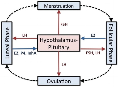
The menstrual cycle consists of the follicular phase, ovulation, and the luteal phase (Figure ) with an average duration of 28 days [Citation37]. During the follicular phase, FSH initiates the development of 6–12 follicles and a dominant follicle is selected to grow to maturity [Citation26, Citation27]. These follicles produce E2 which primes the pituitary to secrete LH in large amounts. At mid-cycle, a rise and fall of LH over a period of five days causes the dominant follicle to release its ovum and this LH surge is necessary for ovulation. The dominant follicle becomes the corpus luteum, which produces E2 and P4 in preparation for pregnancy. If fertilization does not occur, the corpus luteum atrophies which signals the end of one cycle and the beginning of the next.
In mammals such as cows, horses, and sheep, it has been known [Citation11] that multiple follicles of ovulatory size develop during a single reproductive cycle but only one releases an ovum. Because these follicles grow sequentially (e.g. Figure , Panel a), they are described as follicle waves [Citation12]. The growth of two or three follicle waves of this sort is stimulated by separate waves of FSH. Because luteal P4 suppresses a LH surge, the ovulatory follicle arises from the cohort that matures after the corpus luteum has atrophied and P4 has diminished. Baerwald et al. [Citation1, Citation2] have observed follicle waves in normally cycling women. In Baerwald et al. [Citation3], two or three follicle waves were illustrated during one menstrual cycle. These waves are initiated by rises in FSH levels. Specifically, for a two-wave cycle, the first wave is produced by the early follicular phase rise in FSH and the second wave, by the sharp FSH spike concurrent with the LH surge at mid-cycle (Figure , Panel b). The follicle wave corresponding to the mid-cycle FSH spike develops during the luteal phase of the cycle but does not ovulate because of the absence of a luteal LH surge (suppressed by luteal P4) and possibly because the follicle does not reach ovulatory size. When the third wave appears, it develops in response to an unusual late luteal/early follicular rise in FSH (Figure , Panel e) as reported by Baerwald et al. [Citation3].
Figure 2. Graphs are taken from Baerwald et al. [Citation3], based on results from Baerwald et al. [Citation1, Citation2]. Panel (a) depicts two follicle waves per cycle and the corpus luteum (yellow body). Panels (b) and (c) graph corresponding LH, FSH, E2, and P4 concentrations. Two-thirds of the women studied had cycles exhibiting two follicle waves per cycle and their results are shown. Note that two follicle waves per cycle corresponds to two rises in FSH. From Baerwald et al. [Citation3] by permission of Oxford University Press. Human Reproduction Update is published on behalf of the European Society of Human Reproduction and Embryology (ESHRE).
![Figure 2. Graphs are taken from Baerwald et al. [Citation3], based on results from Baerwald et al. [Citation1, Citation2]. Panel (a) depicts two follicle waves per cycle and the corpus luteum (yellow body). Panels (b) and (c) graph corresponding LH, FSH, E2, and P4 concentrations. Two-thirds of the women studied had cycles exhibiting two follicle waves per cycle and their results are shown. Note that two follicle waves per cycle corresponds to two rises in FSH. From Baerwald et al. [Citation3] by permission of Oxford University Press. Human Reproduction Update is published on behalf of the European Society of Human Reproduction and Embryology (ESHRE).](/cms/asset/0c5ba22f-5e25-4b96-b39b-ea57950553a3/tjbd_a_1115564_f0002_c.jpg)
Figure 3. Graphs are taken from Baerwald et al. [Citation3], based on results from Baerwald et al. [Citation1, Citation2]. Panel (d) depicts three follicle waves per cycle and the corpus luteum (yellow body). Panels (e) and (f) graph corresponding LH, FSH, E2, and P4 concentrations. One-third of the women studied had cycles exhibiting three follicle waves per cycle and their results are shown. Note that three follicle waves per cycle corresponds to three rises in FSH. From Baerwald et al. [Citation3] by permission of Oxford University Press. Human Reproduction Update is published on behalf of the ESHRE .
![Figure 3. Graphs are taken from Baerwald et al. [Citation3], based on results from Baerwald et al. [Citation1, Citation2]. Panel (d) depicts three follicle waves per cycle and the corpus luteum (yellow body). Panels (e) and (f) graph corresponding LH, FSH, E2, and P4 concentrations. One-third of the women studied had cycles exhibiting three follicle waves per cycle and their results are shown. Note that three follicle waves per cycle corresponds to three rises in FSH. From Baerwald et al. [Citation3] by permission of Oxford University Press. Human Reproduction Update is published on behalf of the ESHRE .](/cms/asset/ba601477-06ee-4840-a82c-265090ed7414/tjbd_a_1115564_f0003_c.jpg)
In this study, we illustrate follicle waves in normally cycling women by modifying the mathematical model introduced in Harris' thesis [Citation14] and Harris-Clark et al. [Citation15], which consists of 13 nonlinear, delay differential equations. We alter this system by including a single FSH threshold function to stimulate the growth of the first stage of follicular development as suggested by Zeleznik [Citation44]. With a FSH threshold, the follicular phase rise in FSH and the mid-cycle surge in FSH will both promote the development of dominant follicles and the possibility of dual ovulations. To prevent a second dominant follicle, we add follicle atresia which depends on LH and this suppresses the development of a dominant follicle stage during the luteal phase. In her thesis, Margolskee [Citation21] was the first to experiment with FSH thresholds and atresia and to demonstrate the possibility of follicle waves in a mathematical model.
The parameters of our system of differential equations are estimated here using the data of McLachlan et al. [Citation23]. These data resemble the Baerwald hormone profiles in Figure but also include inhibin A which is needed in our model because of its effect on FSH synthesis (Section 2.1). Simulations of our model approximate well the pituitary and ovarian hormone profiles in McLachlan et al. [Citation23]. Also, simulations of the different stages of follicle development exhibit a follicle wave resulting in a dominant follicle during the follicular phase and a second wave of nonovulatory follicles during the early luteal phase similar to those depicted in Figure , Panel (a). Numerical experiments are carried out to show that this model may also produce three follicle waves per cycle. In particular, we input a FSH profile similar to that in Panel (e) of Figure to illustrate that our model can produce three follicle waves like those in Panel (d) of Figure .
An interesting biological question is what conditions permit an ovulation from the second follicle wave and, hence, the possibility of fertilization of two ova at different times during the same menstrual cycle. The occurrence of dizygotic twins [Citation13] in such a case is referred to as superfecundation [Citation17, Citation40]. Our model may be used to illustrate the possibility of superfecundation. By removing the atresia term and making some other parameter modifications, we show that the second follicle wave can result in a second dominant follicle which will elicit a second LH surge and another ovulation.
2. Model development
Many mathematical models for hormonal control of the menstrual cycle track blood levels of hormones produced by the brain and the ovaries during the follicular and luteal phases of the cycle using systems of differential equations. Our model is based on a nonlinear system of 13 delay, differential equations first presented in Harris-Clark et al. [Citation15] which includes the five reproductive hormones LH, FSH, E2, P4, and InhA. Model parameters are estimated using data for 33 normally cycling women in McLachlan et al. [Citation23] which provides average daily blood levels of the 5 hormones over a 31-day month. Because the ovaries respond to daily averages [Citation26], our model lumps the effects of the hypothalamus and the pituitary together and we consider ovarian hormone regulation of the synthesis and release of FSH and LH on a time scale of days (Section 2.1). In addition, because the clearance of the ovarian hormones from the blood is rapid compared to the clearance of the pituitary hormones and compared to the time scale for ovarian development, we assume that the blood levels of the ovarian hormones are at quasi-steady state [Citation19]. Hence, their concentrations are expressed as linear combinations of ovarian stages of the cycle (Section 2.2). These simplifications permit the use of a daily time scale to track hormonal variation during the cycle. Finally, similar to the approach of Harris-Clark et al. [Citation15], we construct our model in three steps: a pituitary system, an ovarian system, and the full system.
2.1. The pituitary system
Four differential equations are used to represent the synthesis, release, and clearance of LH and FSH from the pituitary into the blood under control of the ovarian hormones (Figure ). These equations were derived in Schlosser and Selgrade [Citation34] where the state variables, and
, represent the amounts of LH and FSH in the pituitary reserve pool and the state variables, LH and FSH, represent concentrations in the blood. Assuming that V is constant blood volume, the four equations take the following general form:
(1)
(1)
(2)
(2)
(3)
(3)
(4)
(4)
Figure 4. The brain and the blood compartments for the pituitary model are illustrated. E2, P4, and InhA stimulate (+) and/or inhibit (−) the synthesis and/or release of the pituitary hormones. Clearance from the blood is linear.
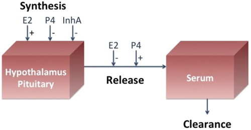
Synthesis and release rates for LH and FSH are described as rational functions of ovarian hormones in which stimulatory effects appear in the numerators and inhibitory effects appear in the denominators. Clinical research has indicated that P4 stimulates the release of LH and FSH into circulation [Citation7] and that low levels of E2 inhibit the release of LH and FSH [Citation38]. Also, it has been shown [Citation20, Citation42] that the high levels of E2 produced by the dominant follicle elicit the mid-cycle LH surge, so the numerator of the LH synthesis term contains a Hill function of E2 to reflect this effect on LH. The inhibins inhibit FSH synthesis [Citation42]. These features are discussed in detail in [Citation34] and [Citation15] where the following system expands Equations (Equation1(1)
(1) )–(Equation4
(4)
(4) ):
(5)
(5)
(6)
(6)
(7)
(7)
(8)
(8)
The data of McLachlan et al. [Citation23] for the ovarian hormones are used to obtained statistical fits for input functions ,
, and
in Equations (Equation5
(5)
(5) )–(Equation8
(8)
(8) ). Thus, in this step of the modelling process, Equations (Equation5
(5)
(5) )–(Equation8
(8)
(8) ) are time-dependent ordinary differential equations which are linear in the state variables,
, LH,
, and FSH. The parameters
,
, and
denote the period of time between when changes in E2, P4, and InhA blood levels occur and changes in the synthesis rates of LH and FSH result. These time delays are used only in the synthesis terms because we assume that hormone synthesis is a more complicated biological process than hormone release. Then, the data of McLachlan et al. [Citation23] for LH and FSH are used to estimate the 16 unknown parameters of Equations (Equation5
(5)
(5) )–(Equation8
(8)
(8) ) as was done in Harris-Clark et al. [Citation15].
2.2. The ovarian system
The ovarian model, first developed by Selgrade and Schlosser [Citation35], describes nine stages in the monthly growth and development of the ovaries. FSH and LH promote the growth of follicular tissue within a stage and the transfer of follicular tissue from one stage to the next. The capacity to produce hormones at each stage of the cycle is assumed to be proportional to the mass of the ovarian follicles or corpus lutea at that stage. The nine stages are as follows:
(RcF) Recruited Stage: FSH-induced recruitment from the preantral pool,
(GrF) Growing Stage: FSH sustaining growth of cohort,
(DomF) Dominant Stage: selection of a dominant follicle,
(
) First Ovulatory Stage: follicle ovulation,
(
(
The increase in mass and transfer of mass for each stage is described by a differential equation which is linear in the state variables with coefficients depending on the pituitary hormones. A transfer term in one equation appears as a growth term in the next equation as follows:
(9)
(9)
(10)
(10)
(11)
(11)
(12)
(12)
(13)
(13)
(14)
(14)
(15)
(15)
(16)
(16)
(17)
(17)
Applying the quasi-steady state assumption as did Bogumil et al. [Citation4, Citation5], we write ovarian hormone concentrations as linear combinations of the stages that secrete these hormones:
(18)
(18)
(19)
(19)
(20)
(20)
The ovarian system of previous models [Citation15, Citation22, Citation35, Citation36] used first-order FSH terms to initiate follicular growth. However, Zeleznik [Citation44] suggests that FSH levels must exceed a threshold to initiate follicular development. Such a threshold effect may be captured mathematically using the Hill function of FSH in Equation (Equation9(9)
(9) ):
This function of FSH has an increasing sigmoidal shaped graph. The Hill coefficient p determines the steepness of the graph, the parameter is the limiting value of the function, and the half-saturation parameter
is the FSH value giving a function value of
. Here we show that parameters may be found so that this single Hill function as it appears in the differential Equation (Equation9
(9)
(9) ) results in the appearance of two follicle waves.
For a normally cycling woman, only the wave occurring in the folliclular phase will result in an ovulating follicle. To prevent a second dominant follicle, we add follicle atresia in Equation (Equation11(11)
(11) ) which depends inversely on LH:
Because luteal P4 inhibits LH synthesis, LH is low during the luteal phase resulting in a larger atresia term. Hence, a luteal phase follicle wave does not produce a dominant follicle and no second ovulation occurs. In Section 5, we show that the removal of this atresia term does result in a second ovulation and the possibility of fraternal twins.
In Equations (Equation9(9)
(9) )–(Equation17
(17)
(17) ),
and
are explicit functions of time t obtained statistically from the pituitary hormone data of [Citation23]. Then, the McLachlan data for E2, P4, and InhA are used to estimate the 32 parameters in Equations (Equation9
(9)
(9) )–(Equation20
(20)
(20) ) as was done in Section 2.1.
2.3. The merged system
The third and final step of model construction is to merge the pituitary system and ovarian system together to create a single 13-dimensional system of differential Equations (Equation5(5)
(5) )–(Equation17
(17)
(17) ) with three auxiliary equations (Equation18
(18)
(18) )–(Equation20
(20)
(20) ). The nonlinear coefficient functions of the inputs in Sections 2.1 and 2.2 now become nonlinear functions of state variables so the system is highly nonlinear. The parameters
,
, and
are discrete time delays so Equations (Equation5
(5)
(5) )–(Equation17
(17)
(17) ) are delay differential equations. The 51 parameters of Equations (Equation5
(5)
(5) )–(Equation20
(20)
(20) ) must be re-estimated using the data of McLachlan et al. [Citation23] but the parameters found in Sections 2.1 and 2.2 are good starting values. Optimized parameters are obtained using least-squares and the Nelder–Mead Simplex method implemented in MATLAB [Citation25] (see [Citation28] for details). These parameters are listed in Table .
3. Model simulations – two follicle waves
Numerical solutions to Equations (Equation5(5)
(5) )–(Equation20
(20)
(20) ) are computed using the delay equations solver DDE23 in MATLAB. Testing a variety of initial conditions indicates that solutions approach a unique stable solution of period approximately 31.5 days. Initial conditions for this stable cycle are listed in Table and are used to plot the follicle stages for two complete cycles in Figure and the four hormones LH, FSH, E2, and P4 against the data of [Citation23] in Figures and . The left panel of Figure displays the first three ovarian follicle stages, the recruited stage RcF, the growing stage GrF, and the dominant stage DomF. RcF and GrF exhibit two follicle waves – a large follicular phase wave which becomes the dominant, ovulatory follicle, and a smaller luteal phase wave. The atresia term in Equation (Equation11
(11)
(11) ) eliminates a luteal phase dominant follicle. In fact, the atresia is so successful at reducing the dominant stage after mid-cycle that all subsequent stages,
through
, are quite small (see the right panel in Figure ).
Figure 5. All ovarian follicle stages for the merged model Equations (Equation5(5)
(5) )–(Equation20
(20)
(20) ) with parameters of Table are shown for two cycles. The model maintains two follicle waves for the recruited RcF and growing GrF stages (left panel). The atresia term reduces the dominant stage DomF after mid-cycle and effectively results in small subsequent ovarian stages (right panel).
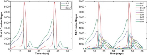
Figure 6. Ovarian hormones E2 and P4 for the merged model Equations (Equation5(5)
(5) )–(Equation20
(20)
(20) ) with parameters of Table are plotted against the McLachlan data [Citation23] for two cycles.
![Figure 6. Ovarian hormones E2 and P4 for the merged model Equations (Equation5(5) ddtRPLH=v0LH+v1LHE2(t−dE)aKmLHa+E2(t−dE)a1+P4(t−dP)KiLH,P−kLH(1+cLH,PP4)RPLH1+cLH,EE2,(5) )–(Equation20(20) InhA=h0+h1DomF+h2Lut2+h3Lut3+h4Lut4.(20) ) with parameters of Table 2 are plotted against the McLachlan data [Citation23] for two cycles.](/cms/asset/d2cfae48-8574-432c-bba9-e146c3fb7213/tjbd_a_1115564_f0006_c.jpg)
Figure 7. Pituitary hormones LH and FSH for the merged model Equations (Equation5(5)
(5) )–(Equation20
(20)
(20) ) with parameters of Table are plotted against the McLachlan data [Citation23] for two cycles.
![Figure 7. Pituitary hormones LH and FSH for the merged model Equations (Equation5(5) ddtRPLH=v0LH+v1LHE2(t−dE)aKmLHa+E2(t−dE)a1+P4(t−dP)KiLH,P−kLH(1+cLH,PP4)RPLH1+cLH,EE2,(5) )–(Equation20(20) InhA=h0+h1DomF+h2Lut2+h3Lut3+h4Lut4.(20) ) with parameters of Table 2 are plotted against the McLachlan data [Citation23] for two cycles.](/cms/asset/2d2017ad-d130-43b2-bd33-6a39c0566e09/tjbd_a_1115564_f0007_c.jpg)
From Equations (Equation18(18)
(18) )–(Equation20
(20)
(20) ) for the ovarian hormones, note that the second follicle wave affects only E2 and this is because of the GrF term in Equation (Equation18
(18)
(18) ). As a result, the luteal E2 peak is higher than the data and almost 80% of the follicular E2 peak (Figure , left panel). Because E2 promotes LH synthesis, Equation (Equation5
(5)
(5) ), there is additional LH in the luteal phase appearing as a small bump in the LH profile (Figure , left panel). P4, which depends on the luteal stages, does not reach the luteal data peak (Figure , right panel) because these stages are small.
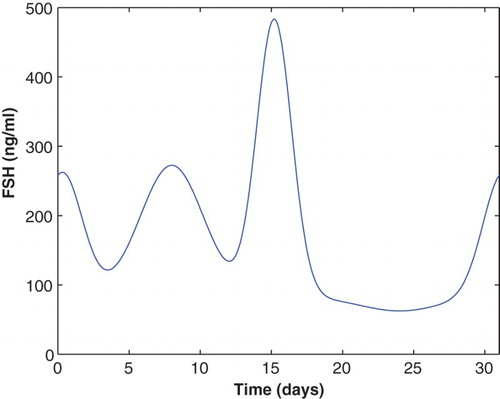
4. Three follicle waves
Baerwald et al. [Citation3] illustrated three follicle waves per cycle depicted in Figure , Panel (d). Each wave corresponds to a different peak in FSH as observed in Figure , Panel (e), where a late luteal rise in FSH is interrupted by an early follicular dip in the FSH graph followed by its normal follicular phase rise. Daily FSH data for such a FSH profile are not available for us to use in a full model simulation. However, in order to test if our model can generate three follicle waves from this type of FSH profile, we use the ovarian model component discussed and implemented in Section 2.2. An input function is obtained from the data of [Citation23] as done in Section 2.2 but a new input for
is defined using negative exponential functions of t to position three appropriately spaced rises as follows:
(21)
(21)
This FSH profile is scaled to be consistent with the McLachlan data and is plotted in Figure .
Figure 8. The FSH input function (Equation21(21)
(21) ) has three distinct rises during one cycle and is used to produce three follicle waves.
These input functions for and
are inserted into the system of differential Equations (Equation9
(9)
(9) )–(Equation17
(17)
(17) ) with auxiliary Equations (Equation18
(18)
(18) )–(Equation20
(20)
(20) ) to produce three follicle waves per cycle (Figure ). The data for E2, P4, and InhA from McLachlan et al. [Citation23] are used to optimize the parameters (see [Citation28] for details) and these parameters are listed in Table . Figure plots model simulations of the ovarian hormones against the data of [Citation23]. Notice that three waves occur for the first two ovarian stages RcF and GrF but the atresia term eliminates the first and third waves in the dominate stage (Figure , left panel). To prevent an early follicular rise in E2 (Figure ), we reduce the parameter
in Equation (Equation18
(18)
(18) ) to one-half of its value for the two-wave model (compare Tables and ).
Figure 9. Follicle stages are plotted for Equations (Equation9(9)
(9) )–(Equation20
(20)
(20) ) where the FSH input (Equation21
(21)
(21) ) has three distinct rises. The parameters are given in Table . The left panel depicts the first three stages of follicle growth and isolates waves in the recruited RcF (−) and the growing GrF (−) stages. Note that DomF (−) exhibits only one wave. The right panel gives the complete set of nine follicle stages.
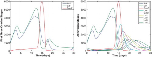
Figure 10. The data of McLachlan et al. [Citation23] for the ovarian hormones are compared to simulations of Equations (Equation9(9)
(9) )–(Equation20
(20)
(20) ) with parameters of Table . The FSH input function (Equation21
(21)
(21) ) with three distinct rises is used.
![Figure 10. The data of McLachlan et al. [Citation23] for the ovarian hormones are compared to simulations of Equations (Equation9(9) ddtRcF=b⋅FSH+c1FSHpKmFp+FSHpRcF−c2LHαRcF,(9) )–(Equation20(20) InhA=h0+h1DomF+h2Lut2+h3Lut3+h4Lut4.(20) ) with parameters of Table 4. The FSH input function (Equation21(21) FSH=82.5+190e−(t−8)210+180e−(t−0.3)20.4+400e−(t−15.2)23−20e−(t−24)215.(21) ) with three distinct rises is used.](/cms/asset/649b7cc7-67ef-46fb-ba7c-ddb3729dbcd3/tjbd_a_1115564_f0010_c.jpg)
5. Superfecundation
Dizygotic twinning may happen when multiple ovulations occur during a single or consecutive menstrual cycles and two oocytes are fertilized [Citation13]. In recent years, the incidence of this has increased partially due to more women receiving fertility treatments and more older women becoming pregnant [Citation5, Citation6, Citation41]. Though rare, dizygotic twins via superfecundation could be a direct consequence of multiple follicle waves per cycle. Superfecundation is the ovulation and fertilization of two oocytes at different times during the same menstrual cycle [Citation17]. This may occur if two follicle waves result in two dominant, ovulatory follicles during the same cycle. Most cases of superfecundation are noticed only when the twins have different fathers because they look drastically different or by chance a paternity test is conducted. A recent child support case was deemed ‘groundbreaking’ because the paternity test on a woman's twins showed that they had different fathers and the father who was being sued only had to pay support for one of the twins [Citation24].
Here we show that removing the atresia term from Equation (Equation11(11)
(11) ) and changing some parameters cause a luteal phase dominant follicle which secretes enough E2 to elicit a second LH surge and a second ovulation. If both oocytes are fertilized, then dizygotic twins may result. First, setting the parameter
to zero removes the atresia term in Equation (Equation11
(11)
(11) ). This permits the growth of a dominant follicle stage during the luteal phase (Figure ) and the resulting secretion of large amounts of luteal E2 (Figure ). E2 promotes the synthesis of LH but P4 inhibits LH (see the first term in Equation Equation5
(5)
(5) ). To guarantee a luteal LH surge (Figure ), we diminish luteal P4 via Equation (Equation19
(19)
(19) ) by decreasing parameter
slightly and parameter
by a factor of 10 (compare Table and Table ). Other ad hoc parameter adjustments are made to insure two LH surges of comparable strength, for example,
is increased and
is decreased. Then, the data for FSH, E2, and InhA from [Citation23] are used to optimize remaining parameters (see [Citation28] for details).
Figure 11. The first three stages of ovarian development for the model of follicle wave superfecundation are plotted for two cycles. The parameters are given in Table . The luteal phase DomF (−) stage produces large amounts of luteal E2 which causes a second LH surge, Figure .
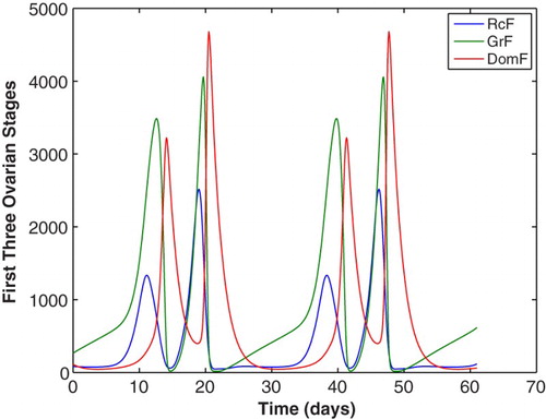
Figure 12. E2 and LH from the model of follicle wave superfecundation is compared to the McLachlan data [Citation28] for two cycles. During one cycle, a second LH surge is present due to increased luteal E2 levels produced by a second dominant follicle. A second LH surge allows for ovulation of the second dominant follicle for potential fertilization resulting in superfecundation.
![Figure 12. E2 and LH from the model of follicle wave superfecundation is compared to the McLachlan data [Citation28] for two cycles. During one cycle, a second LH surge is present due to increased luteal E2 levels produced by a second dominant follicle. A second LH surge allows for ovulation of the second dominant follicle for potential fertilization resulting in superfecundation.](/cms/asset/3779df30-1fbf-4e55-bb94-dbf58f09671a/tjbd_a_1115564_f0012_c.jpg)
6. Sensitivity and bifurcation analyses
Sensitivity analysis measures changes in system behaviour with respect to changes in parameters [Citation43]. The purpose is to identify the parameters that have the largest impact on the dynamical behaviour of the system. The parameters that greatly affect the model output when changed slightly are known as sensitive parameters, while the parameters that have little effect on the model output are known as insensitive parameters [Citation31]. Local sensitivity analysis examines the effects that the system undergoes when each parameter is changed one at a time. Here model outputs of crucial importance are the follicular phase E2 peak because it affects the LH surge and the FSH profile because it determines the follicle waves. So Panza [Citation27] computes a normalized sensitivity coefficient for each model parameter measuring changes in E2 for four days centred at the E2 peak (ranked in Table , column 2) and another coefficient for changes in FSH for one complete cycle (ranked in Table , column 3). The five most sensitive parameters are ranked in Table with being the most sensitive for both model outputs. Notice that the five most sensitive parameters are the same for both outputs. The parameters
,
, and
affect the synthesis of the pituitary hormones, which control ovarian development.
is the half-saturation for the Hill function which promotes the growth of the first follicle stage RcF and α affects the transfer of mass from RcF to GrF (Equation (Equation9
(9)
(9) )). These two are the stages which exhibit follicle wave behaviour.
Table 1. The five most sensitive parameters ranked in order for model Equations (Equation5(5) (5) )–(Equation20(20) (20) ) with parameters from Table . The model output for the second column is E2 peak and for the third column is FSH cycle profile. The five most sensitive parameters are the same for both outputs.
Numerical simulations of Equations (Equation5(5)
(5) )–(Equation20
(20)
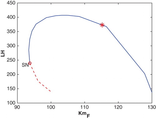
(20) ) with parameters from Table , which were optimized using the data of [Citation23], indicate that the stable cycle is unique (Figures and ). If the sensitive parameters in Table are varied near their best-fit values, the unique stable cycle appears to persist. Using the bifurcation software for delay differential equations, DDEBIFTOOL [Citation10] confirms this suspicion by displaying a simple continuation curve through the best-fit value and no bifurcations nearby (see Figure for the parameter
). Hence, a woman whose reproductive cycle is determined by this parameter set would cycle normally and small perturbations would not significantly disturb her cycle.
Figure 13. This bifurcation diagram plots the maximal LH value along a periodic solution of Equations (Equation5(5)
(5) )–(Equation20
(20)
(20) ) against
with the remaining parameters from Table . SN denotes a saddle-node bifurcation and the * indicates the position of the cycle for best-fit
. The solid blue curve represents stable cycles and the dashed red curve, unstable cycles.
The superfecundation system, Equations (Equation5(5)
(5) )–(Equation20
(20)
(20) ) with parameters from Table , produces dominant follicles DomF in both the follicular and luteal phases of the cycle primarily because of the absence of atresia. Introducing atresia by permitting the atresia coefficient
to be nonzero and by taking
and
results in interesting dynamical behaviour. Increasing
diminishes the dominant follicle and the LH surge during the follicular phase but not the luteal phase (Figure ). For
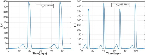
near 20, the follicular phase LH surge is clearly too small to cause ovulation so ovulation occurs only during the luteal phase and the possibility of superfecundation is lost. For a woman whose cycle is described by this situation, her cycle length is normal (here about 30 days) but ovulation occurs much later than mid-cycle. Observe the LH profile in Figure , left panel, where the LH surge occurs at day 19 instead of day 15.
Figure 14. DomF and LH for the superfecundation model for three values of show a diminishing dominant follicle and LH surge during the follicular phase. If
, there is just one ovulation per cycle.
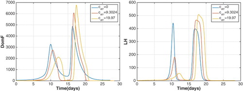
Figure 15. LH profiles for and
illustrating that the period of the stable cycle doubles between these values, that is, a period-doubling bifurcation occurs.
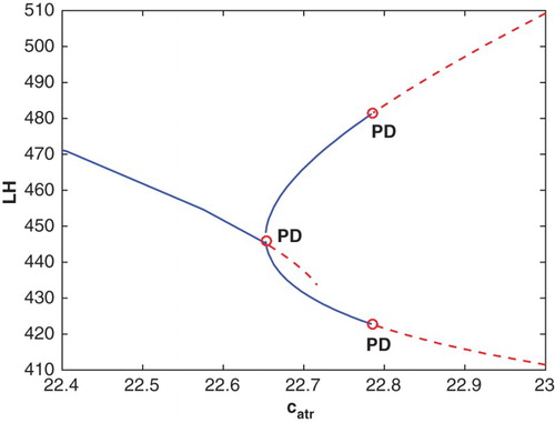
As increases above 20, a cascade of period-doubling bifurcations occurs. At
, the cycle of period 30 days becomes unstable and a stable cycle of about 60 days appears as observed by comparing the LH profiles for
and
(Figure ). Then at
, a second period-doubling bifurcation occurs and a stable cycle of approximately 120 days appears. A portion of the bifurcation diagram showing these two period-doubling bifurcations is drawn in Figure .
Figure 16. The maximal LH value along a periodic solution of Equations (Equation5(5)
(5) )–(Equation20
(20)
(20) ) is plotted against
with
,
, and the remaining parameters from Table . PD denotes period-doubling bifurcations which occur at
and
. The solid blue curves represent stable cycles and the dashed red curves, unstable cycles.
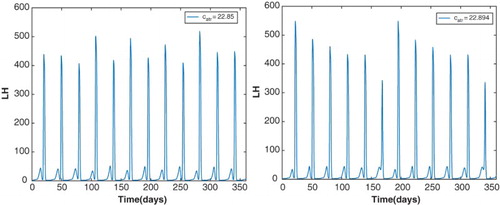
The sequence of bifurcations as increases from 22.5 to 23 resembles the standard period-doubling route to chaos [Citation9] with a chaotic cycle at
and a period-6 window around
(Figure ). The left panel of Figure plots a menstrual cycle which is not exactly periodic but there are 12 LH surges per year. The right panel of Figure plots a stable cycle of period about 180 days which is roughly six times the period of the cycle at
. Such a interval in a bifurcation diagram is referred to as a period-6 window. A woman whose reproductive cycle is represented by this parameter regime could experience unpredictable cycles. This indicates that the two models corresponding to the parameters of Table or of Table with atresia are quite different. The model corresponding to Table depicts a normally cycling woman with hormone levels consistent with data in the literature [Citation23] and exhibiting two follicle waves per cycle. The model corresponding to Table with atresia added represents a woman who may experience superfecundation but also whose cycle is easily disturbed by small variations in follicle atresia.
Figure 17. The left panel illustrates the LH profile of a stable, chaotic cycle at . There are 12 LH surges per year but they do not have the same magnitude. The right panel plots the LH profile of a stable cycle of period approximately 180 days at
. This indicates the presence of a period-6 window in the
bifurcation diagram.
7. Summary and discussion
This study describes a system of 13 nonlinear, delay differential equations with 51 parameters which models the phenomenon of follicle waves in normally cycling women first observed by Baerwald et al. [Citation1–3]. Using model Equations (Equation5(5)
(5) )–(Equation20
(20)
(20) ), we exhibit menstrual cycles with two or three follicle waves corresponding to the number of rises in blood levels of FSH. Simulations with the parameters of Table depict two follicle waves per cycle and resulting hormone profiles accurately approximate the data of [Citation23] (Figures and ). Data with three distinctive rises in FSH are not available but we use the input function plotted in Figure with three FSH hills timed to correspond to the hills of Panel (e) in Figure from [Citation3]. This input function in Equations (Equation9
(9)
(9) )–(Equation20
(20)
(20) ) with the parameters of Table causes the formation of three follicle waves as depicted in Figure and the resulting ovarian hormones are plotted against the data of [Citation23] in Figure . We conjecture that variations in InhB levels during the late luteal to early follicular transition might cause a FSH profile like Figure , Panel (e), but we do not have data to substantiate this conjecture. Since InhB inhibits FSH synthesis and is prominent during the late luteal to early follicular transition, decreases in InhB would result in increases in FSH.
The inclusion of an atresia term in Equation (Equation11(11)
(11) ) prevents more than one ovulation per cycle. We show that removing this term and making some parameter adjustments permit two ovulations per cycle and, hence, the possibility of dizygotic twins via superfecundation. Simulations of Equations (Equation5
(5)
(5) )–(Equation20
(20)
(20) ) with parameters of Table exhibit two dominant follicles per cycle (Figure ) and two LH surges (Figure , right panel). This situation results in two ovulations per cycle. Introducing atresia back into the superfecundation system by taking
and
and increasing
from zero, causes the loss of superfecundation and a cascade of period-doubling bifurcations. This system may produce erratic menstrual cycle behaviour. Hence, although model equations are the same, the two models corresponding to the parameters of Table or of Table with atresia have different dynamical behaviours and represent women with noticeably different reproductive hormone profiles.
Acknowledgements
The authors thank Dr Angela R. Baerwald of University of Saskatchewan for helpful communications.
Disclosure statement
No potential conflict of interest was reported by the authors.
Additional information
Funding
References
- A.R. Baerwald, G.P. Adams, and R.A. Pierson, A new model for ovarian follicular development during the human menstrual cycle, Fertil. Steril. 80 (2003), pp. 116–122. doi: 10.1016/S0015-0282(03)00544-2
- A.R. Baerwald, G.P. Adams, and R.A. Pierson, Characterization of ovarian follicular wave dynamics in women, Biol. Reprod. 69 (2003), pp. 1023–1031. doi: 10.1095/biolreprod.103.017772
- A.R. Baerwald, G.P. Adams, and R.A. Pierson, Ovarian antral folliculogenesis during the human menstrual cycle: A review, Hum. Reprod. Update 18 (2012), pp. 73–91. doi: 10.1093/humupd/dmr039
- R.J. Bogumil, M. Ferin, J. Rootenberg, L. Speroff, and R.L. Vande Wiele, Mathematical studies of the human menstrual cycle. I: Formulation of a mathematical model, J. Clin. Endocrinol. Metab. 35 (1972), pp. 126–143. doi: 10.1210/jcem-35-1-126
- R.J. Bogumil, M. Ferin, and R.L. Vande Wiele, Mathematical studies of the human menstrual cycle. II: Simulation performance of a model of the human menstrual cycle, J. Clin. Endocrinol. Metab. 35 (1972), pp. 144–156. doi: 10.1210/jcem-35-1-144
- R. Bortolus, F. Parazzini, L. Chatenoud, G. Benzi, M.M. Bianchi, and A. Marini, The epidemiology of multiple births, Hum. Reprod. Update 5 (1999), pp. 179–187. doi: 10.1093/humupd/5.2.179
- R.J. Chang and R.B. Jaffe, Progesterone effects on gonadotropin release in women pretreated with estradiol, J. Clin. Endocrinol. Metab. 47 (1978), pp. 119–125. doi: 10.1210/jcem-47-1-119
- C.Y. Chen and J.P. Ward, A mathematical model for the human menstrual cycle, Math. Med. Biol. 31 (2014), pp. 65–86. doi: 10.1093/imammb/dqs048
- R.L. Devaney, A First Course in Chaotic Dynamical Systems: Theory and Experiment, Westview Press, Boulder, 1992.
- K. Engelborghs, T. Luzyanina, and D. Roose, Numerical bifurcation analysis of delay differential equations, J. Comput. Appl. Math. 125 (2000), pp. 265–275. doi: 10.1016/S0377-0427(00)00472-6
- J.E. Fortune, Ovarian follicular growth and development in mammals, Biol. Reprod. 50 (1994), pp. 225–232. doi: 10.1095/biolreprod50.2.225
- O.J. Ginther, M.A. Beg, E.L. Gastal, M.O. Gastal, A.R. Baerwald, and R.A. Pierson, Systemic concentrations of hormones during the development of follicular waves in mares and women: A comparative study, Reproduction 130 (2005), pp. 379–388. doi: 10.1530/rep.1.00757
- J.G. Hall, Twinning, Lancet 362 (2003), pp. 735–743. doi: 10.1016/S0140-6736(03)14237-7
- L.A. Harris, Differential equation models for the hormonal regulation of the menstrual cycle, Ph.D. thesis, North Carolina State University, Raleigh, North Carolina, 2001. Available at www.lib.ncsu.edu/resolver/1840.16/4693.
- L. Harris-Clark, P.M. Schlosser, and J.F. Selgrade, Multiple stable periodic solutions in a model for hormonal control of the menstrual cycle, Bull. Math. Biol. 65 (2003), pp. 157–173. doi: 10.1006/bulm.2002.0326
- J. Hotchkiss and E. Knobil, The menstrual cycle and its neuroendocrine control, in The Physiology of Reproduction, Second Edition, E. Knobil and J.D. Neill, eds., Raven Press, Ltd., New York, 1994, pp. 711–750.
- W.H. James, Gestational age in twins, Arch. Dis. Child. 55 (1980), pp. 281–284. doi: 10.1136/adc.55.4.281
- F.J. Karsch, D.J. Dierschke, R.F. Weick, T. Yamaji, J. Hotchkiss, and E. Knobil, Positive and negative feedback control by estrogen of luteinizing hormone secretion in the rhesus monkey, Endocrinology 92 (1973), pp. 799–804. doi: 10.1210/endo-92-3-799
- J. Keener and J. Sneyd, Mathematical Physiology I: Cellular Physiology, 2nd ed., Springer-Verlag, New York, 2009.
- J.H. Liu and S.S.C. Yen, Induction of midcycle gonadotropin surge by ovarian steroids in women: A critical evaluation, J. Clin. Endocrinol. Metab. 57 (1983), pp. 797–802. doi: 10.1210/jcem-57-5-1087
- A. Margolskee, A whole life model of the human menstrual cycle, Ph.D thesis, North Carolina State University, 2013. Available at http://repository.lib.ncsu.edu/ir/handle/1840.16/8672.
- A. Margolskee and J.F. Selgrade, Dynamics and bifurcation of a model for hormonal control of the menstrual cycle with inhibin delay, Math. Biosci. 234 (2011), pp. 95–107. doi: 10.1016/j.mbs.2011.09.001
- R.I. McLachlan, N.L. Cohen, K.D. Dahl, W.J. Bremner, and M.R. Soules, Serum inhibin levels during the periovulatory interval in normal women: Relationships with sex steroid and gonadotrophin levels, Clin. Endocrinol. 32 (1990), pp. 39–48. doi: 10.1111/j.1365-2265.1990.tb03748.x
- B. Mueller, Paternity case for a New Jersey mother of twins bears unexpected results: Two fathers, New York Times (2015), May 8, A20.
- J.A. Nelder and R. Mead, A simplex method for function minimization, Comput. J. 7 (1965), pp. 308–313. doi: 10.1093/comjnl/7.4.308
- W.D. Odell, The reproductive system in women, in Endocrinology, L.J. DeGroot, ed., Grune & Stratton, New York, 1979, pp. 1383–1400.
- S.R. Ojeda, Female reproductive function, in Textbook of Endocrine Physiology, 2nd ed., J.E. Griffin and S.R. Ojeda, eds., Oxford University Press, Oxford, 1992, pp. 134–188.
- N.M. Panza, Modeling follicle wave dynamics in the menstrual cycle, Ph.D. thesis, North Carolina State University, 2015. Available at http://repository.lib.ncsu.edu/ir/bitstream/1840.16/10447/1/etd.pdf.
- R.D. Pasteur and J.F. Selgrade, A deterministic, mathematical model for hormonal control of the menstrual cycle, in Understanding the Dynamics of Biological Systems: Lessons Learned from Integrative Systems Biology, W. Dubitzky, J. Southgate, and H. Fuss, eds., Springer, London, 2011, pp. 38–58.
- L. Plouffe Jr. and S.N. Luxenberg, Biological modeling on a microcomputer using standard spreadsheet and equation solver programs: The hypothalamic-pituitary-ovarian axis as an example, Comput. Biomed. Res. 25 (1992), pp. 117–130. doi: 10.1016/0010-4809(92)90015-3
- S.R. Pope, L.M. Ellwein, C.L. Zapata, V. Novak, C.T. Kelley, and M.S. Olufsen, Estimation and identification of parameters in a lumped cerebrovascular model, Math. Biosci. Eng. 6 (2009), pp. 93–115. doi: 10.3934/mbe.2009.6.93
- I. Reinecke and P. Deuflhard, A complex mathematical model of the human menstrual cycle, J. Theor. Biol. 247 (2007), pp. 303–330. doi: 10.1016/j.jtbi.2007.03.011
- S. Röblitz, C. Stötzel, P. Deuflhard, H.M. Jones, D-O. Azulay, P.H. van der Graff, and S.W. Martin, A mathematical model of the human menstrual cycle for the administration of GnRH analogues, J. Theor. Biol. 321 (2013), pp. 8–27. doi: 10.1016/j.jtbi.2012.11.020
- P.M. Schlosser and J.F. Selgrade, A model of gonadotropin regulation during the menstrual cycle in women: Qualitative features, Environ. Health Perspect. 108(Suppl 5) (2000), pp. 873–881. doi: 10.1289/ehp.00108s5873
- J.F. Selgrade and P.M. Schlosser, A model for the production of ovarian hormones during the menstrual cycle, Fields Inst. Commun. 21 (1999), pp. 429–446.
- J.F. Selgrade, L.A. Harris, and R.D. Pasteur, A model for hormonal control of the menstrual cycle: Structural consistency but sensitivity with regard to data, J. Theor. Biol. 260 (2009), pp. 572–580. doi: 10.1016/j.jtbi.2009.06.017
- A.E. Treloar, R.E. Boynton, B.G. Behn, and B.W. Brown, Variation of the human menstrual cycle through reproductive life, Int. J. Fertil. 12 (1967), pp. 77–126.
- C.C. Tsai and S.S.C. Yen, The effects of ethinyl estradiol administration during early follicular phase of the cycle on the gonadotropin levels and ovarian function, J. Clin. Endocrinol. 33 (1971), pp. 917–923. doi: 10.1210/jcem-33-6-917
- C.F. Wang, B.L. Lasley, A. Lein, and S.S.C. Yen, The functional changes of the pituitary gonadotrophs during the menstrual cycle, J. Clin. Endocrinol. Metab. 42 (1976), pp. 718–728. doi: 10.1210/jcem-42-4-718
- R.E. Wenk, T. Houtz, M. Brooks, and F.A. Chiafari, How frequent is heteropaternal superfecundation? Acta Geneticae Medicae et Gemellologiae 41 (1992), pp. 43–47.
- T. Westergaard, J. Wohlfahrt, P. Aaby, and M. Melbye, Population based study of rates of multiple pregnancies in Denmark 1980–94, BMJ 314 (1997), pp. 775–779. doi: 10.1136/bmj.314.7083.775
- S.S.C. Yen, The human menstrual cycle: Neuroendocrine regulation, in Reproductive Endocrinology. Physiology, Pathophysiology and Clinical Management, 4th ed., S.S.C. Yen, R.B. Jaffe, and R.L. Barbieri, eds., W.B. Saunders Co., Philadelphia, 1999, pp. 191–217.
- H. Yue, M. Brown, J. Knowles, H. Wang, D.S. Broomhead, and D.B. Kell, Insights into the behaviour of systems biology models from dynamic sensitivity and identifiability analysis: a case study of an NF-κB signalling pathway, Mol. BioSyst. 2 (2006), pp. 640–649. doi: 10.1039/b609442b
- A.J. Zeleznik, The physiology of follicle selection, Reprod. Biol. Endocrin. 2 (2004), pp. 31–37. doi: 10.1186/1477-7827-2-31
- A.J. Zeleznik and D.F. Benyo, Control of follicular development, corpus luteum function, and the recognition of pregnancy in higher primates, in The Physiology of Reproduction, 2nd ed., E. Knobil and J.D. Neill, eds., Raven Press, Ltd., New York, 1994, pp. 751–782.