A juvenile–adult population model: climate change, cannibalism, reproductive synchrony, and strong Allee effects

ABSTRACT

We study a discrete time, structured population dynamic model that is motivated by recent field observations concerning certain life history strategies of colonial-nesting gulls, specifically the glaucous-winged gull (Larus glaucescens). The model focuses on mechanisms hypothesized to play key roles in a population's response to degraded environment resources, namely, increased cannibalism and adjustments in reproductive timing. We explore the dynamic consequences of these mechanics using a juvenile–adult structure model. Mathematically, the model is unusual in that it involves a high co-dimension bifurcation at $R_0=1$ which, in turn, leads to a dynamic dichotomy between equilibrium states and synchronized oscillatory states. We give diagnostic criteria that determine which dynamic is stable. We also explore strong Allee effects caused by positive feedback mechanisms in the model and the possible consequence that a cannibalistic population can survive when a non-cannibalistic population cannot.

KEYWORDS:

• Structured population dynamics
• bifurcation
• equilibrium
• synchronous cycles
• imprimitive projection matrix models
• cannibalism
• reproductive synchrony

1. Introduction

Cannibalism is a life history trait found in a wide variety of animals, ranging from protozoans and invertebrates to all major vertebrate classes [15]. Overcrowding and stress can promote cannibalism, but poor food quality and lack of adequate food are the most important reasons for its occurrence [13,16,22]. A degradation of food resources and decreases in their availability are often a result of environmental and climate changes.

For example, increases in sea surface temperature (SST) associated with El Niño-Southern Oscillation (ENSO) events depress marine food webs. While egg and chick cannibalism occurs commonly among colonial-nesting gulls, a recent study demonstrated that egg cannibalism among glaucous-winged gulls (Larus glaucescens) and glaucous-winged × western gull (L. glaucescens ×occidentalis) hybrids increased in response to impoverished food supplies resulting from ENSO-related high SST events [17]. A single cannibalized egg provides almost half the daily energy needs for these birds. Thus, cannibalism implies a negative feedback on juvenile survival, but a positive feedback to adult survival.

In the same colonies of gulls, another behavioural correlate to increased mean SST was reported in [18]. An every-other-day egg laying synchrony was observed to occur in breeding seasons in years of El Niño induced high mean SST. The Fraser Darling Effect [12] states that seasonal reproductive synchrony in colonial birds may confer a selective advantage by means of predator satiation. Similarly, Henson et al. [19] hypothesized that every-other-day ovulation synchrony in gulls may be a response that confers a selective advantage by means of cannibal satiation.

In this paper we derive and analyse a discrete-time, structured population dynamic model that is designed to investigate these life history phenomena. The model is not intended to model gull colony dynamics, but instead to investigate the dynamic consequences of cannibalism of juveniles by adults in response to decreased environmental food resources and reproductive synchrony in response to cannibalism.

The model is derived in Section 2. The model poses interesting and challenging mathematical problems because the projection matrix is imprimitive, a fact that complicates the bifurcation that occurs at $R_0=1$ where the extinction equilibrium destabilizes. In Section 3 we present theorems for a generalized version of the model that describe this bifurcation and its simultaneous creation of both positive equilibria and 2-cycles, the latter of which implies reproductive synchrony. These theorems provide diagnostic quantities that determine which of these bifurcating states is stable/unstable as well as their direction of bifurcation. Applications are given in Section 4 which both illustrate the mathematical theorems and the nature of this bifurcation and which investigate the biological consequences that are possible from increased cannibalism due to decreased environmental food resource availability.

2. Model preliminaries

To investigate reproductive synchrony of adults, we classify the adults in our structured population dynamic model into two classes: those adults who reproduce during the next interval of time and those adults who do not. We refer to these as classes of reproductively active adults and reproductively inactive adults respectively. The graph theoretic representation of our model is shown in Figure 1. The projection matrix associated with this model, which maps the demographic vector $\overline{x}=\left(\begin{array}{c}{x}_1\\ x_2\\ x_3\end{array}\right)=\left(\begin{array}{c}\mathrm{juveniles}\\ \mathrm{reproductively}\mathrm{active}\mathrm{adults}\\ \mathrm{reproductively}\mathrm{inactive}\mathrm{adults}\end{array}\right)$ from time t to t+1 (where the unit of time is the juvenile maturation period), is $P=\left(\begin{array}{ccc}0& b& 0\\ s_1& 0& s_{3}g\\ 0& s_2& s_3(1-g)\end{array}\right).$ Here b is the adult per capita fecundity rate, $s_1$ is the survival probability of a juvenile, $s_2$ is the survival probability of a reproductive adult, and $s_3$ is the survival probability of a reproductively inactive adult. The fraction g is the probability that a reproductively inactive adult will be reproductively active at the next time unit. Thus $b>0,0<s_i<1,0\le g\le 1.$

Figure 1. A juvenile-adult life cycle graph.

Before we investigate the interplay of juvenile cannibalism by adults and reproductive synchrony (Section 4), we consider an example model that illustrates the mathematical issues involved in the model with regard to reproductive synchrony alone. In this example, reproductively active adults regulate their fecundity and the probability g of transition from reproductive inactivity. The projection matrix (1) $P\left(\overline{x}\right)=\left(\begin{array}{ccc}0& b\frac{1}{1+c_2{x}_2}& 0\\ s_1& 0& s_3\frac{1}{1+c_g{x}_2}\\ 0& s_2& s_3\left(1-\frac{1}{1+c_g{x}_2}\right)\end{array}\right)$(1) assumes density regulated fecundity by means of a standard Beverton–Holt (discrete logistic) functional and that the probability an inactive adult will become active is $g=\frac{1}{1+c_g{x}_2}.$ This means that if there are no active adults at time t ($x_2=0$) then all inactive adults will become active at time t+1 (since g=1) and that if the number of active adults $x_2$ present at time t increases then the fraction of inactive adults that become active at time t+1 will decrease. The resulting nonlinear matrix equation [1] (2) $\overline{x}(t+1)=P\left(\overline{x}\right(t\left)\right)\overline{x}\left(t\right),$(2) which maps the closure ${\overline{R}}_{+}^3$ of the positive cone $R_{+}^3$ into itself, is described by the system of difference equations (3a) $\begin{array}{r}{x}_1(t+1)=b\frac{1}{1+c_2{x}_2\left(t\right)}{x}_2\left(t\right),\end{array}$(3a) (3b) $\begin{array}{r}{x}_2(t+1)=s_1{x}_1\left(t\right)+s_3\frac{1}{1+c_g{x}_2\left(t\right)}{x}_3\left(t\right),\end{array}$(3b) (3c) $\begin{array}{r}{x}_3(t+1)=s_2{x}_2\left(t\right)+s_3\left(1-\frac{1}{1+c_g{x}_2\left(t\right)}\right)x_3\left(t\right).\end{array}$(3c) The Jacobian evaluated at the extinction equilibrium $\overline{x}=\overline{0}$ is (4) $P\left(\overline{0}\right)=\left(\begin{array}{ccc}0& b& 0\\ s_1& 0& s_3\\ 0& s_2& 0\end{array}\right).$(4) This is a non-negative, irreducible matrix whose spectral radius r is, by Perron–Frobenius theory, a simple, positive, dominant eigenvalue. By the linearization principle [14], the extinction equilibrium is (locally asymptotically) stable if r<1 and is unstable if r>1. The dominant eigenvalue of Equation (4(4) $P\left(\overline{0}\right)=\left(\begin{array}{ccc}0& b& 0\\ s_1& 0& s_3\\ 0& s_2& 0\end{array}\right).$(4) ) is $r=\sqrt{b{s}_1+s_2{s}_3}.$ Note that r and the inherent net reproduction number (5) $R_0=b\frac{s_1}{1-s_2{s}_3}$(5) are on the same side of 1. (This is an example of general theorems in [10,21].) Thus,

• the extinction equilibrium is (locally asymptotically) stable if $R_0<1$ and is unstable if $R_0>1$.

Using comparison arguments (similar to those found in [3]) one can show

• all solutions $\overline{x}\left(t\right)$ in ${\overline{R}}_{+}^3$ are bounded;

• if $R_0<1$ then solutions $\overline{x}\left(t\right)$ with initial conditions in ${\overline{R}}_{+}^3$ satisfy $\underset{t\to +\mathrm{\infty }}{lim}\parallel \overline{x}\left(t\right)\parallel =0$. Thus, the extinction equilibrium is globally asymptotically stable on ${\overline{R}}_{+}^3$.

By a theorem in [20] we have a stronger result than instability when $R_0>1,$ namely

• the model is uniformly persistent on ${\overline{R}}_{+}^3$ with respect to the extinction equilibrium $\overline{x}=\overline{0}$ when $R_0>1$,

by which is meant that all solutions with initial conditions in ${\overline{R}}_{+}^3\mathrm{\setminus }\left\{0\right\}$ satisfy $lim\underset{t\to +\mathrm{\infty }}{inf}\parallel \overline{x}\left(t\right)\parallel =lim\underset{t\to +\mathrm{\infty }}{inf}\sum _{i=1}^3\left|x_i\right(t\left)\right|\ge \epsilon$ for some $\epsilon >0$ (independent of initial conditions). What can be said about the asymptotic state of a population when $R_0>1$? A look at the equilibrium equations associated with Equation (3(3a) $\begin{array}{r}{x}_1(t+1)=b\frac{1}{1+c_2{x}_2\left(t\right)}{x}_2\left(t\right),\end{array}$(3a) ) shows¹

• if $R_0>1$ then there exists a unique non-extinction equilibrium $\overline{x}\in R_{+}^3$ for each $R_0>1$.

The facts in the bulleted statements above are an example of the fundamental bifurcation theorem for nonlinear matrix models, that a continuum of non-extinction equilibria bifurcate from the extinction equilibrium $\overline{x}=\overline{0}$ at $R_0=1$ [3,6]. This theorem also asserts, under a key assumption, that a forward bifurcation, such as occurs in this example, gives rise to (locally asymptotically) stable non-extinction equilibria (at least for $R_0⪆1$). The key assumption is that the inherent projection matrix $P\left(\overline{0}\right)$ is primitive, that is, its dominant eigenvalue r is strictly dominant. This is not true for Equation (4(4) $P\left(\overline{0}\right)=\left(\begin{array}{ccc}0& b& 0\\ s_1& 0& s_3\\ 0& s_2& 0\end{array}\right).$(4) ), whose eigenvalues are $r=\pm \sqrt{b{s}_1+s_2{s}_3}$ and 0.

In general, for models with imprimitive projection matrices the direction of bifurcation does not alone determine the stability of the bifurcating non-extinction equilibria, as it does for models with primitive projection matrices (see [8] ). The mathematical reason for this is the simultaneous departure from the unit complex circle of more than one eigenvalue as r (equivalently $R_0$) increases through 1. In the example under consideration here, two eigenvalues simultaneously leave the unit complex circle through 1 and $-1$. The destabilization caused by the eigenvalue leaving through $-1$ gives rise to the bifurcation of periodic 2-cycles, which serve as an alternative asymptotic state to the non-extinction equilibria. In this example, the 2-cycles can be calculated explicitly by noting the existence of certain orbits on the boundary $\mathrm{\partial }{R}_{+}^3$ of the positive cone of the form (6) $\left(\begin{array}{c}0\\ +\\ 0\end{array}\right)\to \left(\begin{array}{c}+\\ 0\\ +\end{array}\right)\to \left(\begin{array}{c}0\\ +\\ 0\end{array}\right)\to \left(\begin{array}{c}+\\ 0\\ +\end{array}\right)\to \left(\begin{array}{c}0\\ +\\ 0\end{array}\right)\to \cdots$(6) A periodic 2-cycle of this form, which we call a synchronous 2-cycle, is a fixed point of the composite $\left(\begin{array}{c}0\\ x_2\\ 0\end{array}\right)\to \left(\begin{array}{c}b\frac{x_2}{1+c_2{x}_2}\\ 0\\ s_2{x}_2\end{array}\right)\to \left(\begin{array}{c}0\\ s_2{s}_3{x}_2+b{s}_1\frac{x_2}{1+c_2{x}_2}\\ 0\end{array}\right)$ that is, is given by the positive root $x_2$ of the equation $x_2=s_2{s}_3{x}_2+b{s}_1\frac{x_2}{1+c_2{x}_2}$ which is $x_2=\frac{1}{c_2}(R_0-1).$

• For $R_0>1$ there exists a (unique positive) synchronous 2-cycle consisting of the two points

(7) $\left(\begin{array}{c}0\\ \frac{1}{c_2}(R_0-1)\\ 0\end{array}\right)⟷\left(\begin{array}{c}\frac{1-s_2{s}_3}{s_1}\frac{1}{c_2}(R_0-1)\\ 0\\ s_2\frac{1}{c_2}(R_0-1)\end{array}\right).$(7)

Notice that the synchronous 2-cycles (7(7) $\left(\begin{array}{c}0\\ \frac{1}{c_2}(R_0-1)\\ 0\end{array}\right)⟷\left(\begin{array}{c}\frac{1-s_2{s}_3}{s_1}\frac{1}{c_2}(R_0-1)\\ 0\\ s_2\frac{1}{c_2}(R_0-1)\end{array}\right).$(7) ) describe a state of reproductive synchrony in that temporally all adults are alternatively reproductive active and inactive. This is sharp contrast to the bifurcating non-extinction equilibria, which also exist for $R_0>1$, in which there are both active and inactive adults present at each point of time. Thus, this motivating example contains both of these reproductive strategies and the question becomes which is realizable, that is, which is stable, or more to the point under what conditions will the synchronous 2-cycles be stable and under what conditions will the non-extinction equilibria be stable? We will leave the answer to this question for the next section in which such conditions are provided for a more general model, one that allows for more general nonlinearities and density effects including those associated with adult cannibalism of juveniles.

3. A general model

In this section we consider a generalization of the model with projection matrix (1(1) $P\left(\overline{x}\right)=\left(\begin{array}{ccc}0& b\frac{1}{1+c_2{x}_2}& 0\\ s_1& 0& s_3\frac{1}{1+c_g{x}_2}\\ 0& s_2& s_3\left(1-\frac{1}{1+c_g{x}_2}\right)\end{array}\right)$(1) ) in which density effects are allowed into all demographic parameters. Specifically, the projection matrix is (8) $P\left(\overline{x}\right)=\left(\begin{array}{ccc}0& b{p}_{12}\left(\overline{x}\right)& 0\\ s_1{p}_{21}\left(\overline{x}\right)& 0& s_3{p}_{23}\left(\overline{x}\right)\\ 0& s_2{p}_{32}\left(\overline{x}\right)& s_3{p}_{33}\left(\overline{x}\right)\end{array}\right),$(8) where the nonlinear factors $p_{ij}$ satisfy the smoothness assumptions

H1: $p_{ij}\in C^2(\mathrm{\Omega },{\overline{R}}_{+}^3)$ where Ω is an open set in $R^3$ containing ${\overline{R}}_{+}^3$ such that $0\le s_1{p}_{21}\left(\overline{x}\right),s_3{p}_{23}\left(\overline{x}\right),s_2{p}_{32}\left(\overline{x}\right),s_3{p}_{33}\left(\overline{x}\right)\le 1$

and the conditions

H2: $p_{ij}(0,0,0)=1$ and $p_{23}\left(\overline{x}\right)\equiv 1$ for all $\overline{x}\in {\overline{R}}_{+}^3$ with $x_2=0$.

The first condition in H2 insures that b and $s_i$ are inherent (i.e. density free) demographic parameters. The second condition in H2 expresses the assumption that if no adults are reproductively active at time t then all inactive adults will become active at time t+1.

It is up to the modeler to specify the properties of the terms $p_{ij}\left(\overline{x}\right)$ (which we sometimes denote by $p_{ij}(x_1,x_2,x_3)$) as functions of $\overline{x}$ that reflect the biological and environmental mechanisms of interest, such as the familiar negative feedback effects of population density on fecundity and survival. In the next section we will model the effects of cannibalism of juveniles by adults (both positive and negative).

The matrix (1(1) $P\left(\overline{x}\right)=\left(\begin{array}{ccc}0& b\frac{1}{1+c_2{x}_2}& 0\\ s_1& 0& s_3\frac{1}{1+c_g{x}_2}\\ 0& s_2& s_3\left(1-\frac{1}{1+c_g{x}_2}\right)\end{array}\right)$(1) ) is non-negative and irreducible. The inherent projection matrix $P\left(\overline{0}\right)$, because of H2, is given by Equation (4(4) $P\left(\overline{0}\right)=\left(\begin{array}{ccc}0& b& 0\\ s_1& 0& s_3\\ 0& s_2& 0\end{array}\right).$(4) ). Moreover $P\left(\overline{0}\right)$ is the Jacobian of the nonlinear map defined by Equation (1(1) $P\left(\overline{x}\right)=\left(\begin{array}{ccc}0& b\frac{1}{1+c_2{x}_2}& 0\\ s_1& 0& s_3\frac{1}{1+c_g{x}_2}\\ 0& s_2& s_3\left(1-\frac{1}{1+c_g{x}_2}\right)\end{array}\right)$(1) ) evaluated at $\overline{x}=\overline{0}$. As a result, the extinction equilibrium $\overline{x}=\overline{0}$ is stable if $R_0<1$ and unstable if $R_0>1,$ where $R_0$ is given by Equation (5(5) $R_0=b\frac{s_1}{1-s_2{s}_3}$(5) ). Using this fact and results in [20], we have the following theorem concerning the extinction equilibrium.

Theorem 1.

Assume H1 and H2. For the nonlinear matrix model with projection (8(8) $P\left(\overline{x}\right)=\left(\begin{array}{ccc}0& b{p}_{12}\left(\overline{x}\right)& 0\\ s_1{p}_{21}\left(\overline{x}\right)& 0& s_3{p}_{23}\left(\overline{x}\right)\\ 0& s_2{p}_{32}\left(\overline{x}\right)& s_3{p}_{33}\left(\overline{x}\right)\end{array}\right),$(8) ) the extinction equilibrium $\overline{x}=\overline{0}$ is $($locally asymptotically stable$)$ if $R_0<1$ and unstable if $R_0>1$. Furthermore, if $R_0>1,$ then the model is uniformly persistent with respect to $\overline{x}=\overline{0}$.

3.1. Bifurcation of equilibria at $R_0=1$

The destabilization of the equilibrium $\overline{x}=\overline{0}$ as $R_0$ (equivalently r) increases through 1 signals that a bifurcation occurs that creates new equilibrium states. This is well known for general nonlinear matrix models (of any dimension) when the projection matrix is primitive [3,8]. When the projection matrix is imprimitive, however, the bifurcation can be (and usually is) more complicated, as we will see for the case (8(8) $P\left(\overline{x}\right)=\left(\begin{array}{ccc}0& b{p}_{12}\left(\overline{x}\right)& 0\\ s_1{p}_{21}\left(\overline{x}\right)& 0& s_3{p}_{23}\left(\overline{x}\right)\\ 0& s_2{p}_{32}\left(\overline{x}\right)& s_3{p}_{33}\left(\overline{x}\right)\end{array}\right),$(8) ). First, we need some definitions.

We can write the projection matrix (8(8) $P\left(\overline{x}\right)=\left(\begin{array}{ccc}0& b{p}_{12}\left(\overline{x}\right)& 0\\ s_1{p}_{21}\left(\overline{x}\right)& 0& s_3{p}_{23}\left(\overline{x}\right)\\ 0& s_2{p}_{32}\left(\overline{x}\right)& s_3{p}_{33}\left(\overline{x}\right)\end{array}\right),$(8) ) as (9) $P\left(\overline{x}\right)=\left(\begin{array}{ccc}0& R_0\frac{1-s_2{s}_3}{s_1}{p}_{12}\left(\overline{x}\right)& 0\\ s_1{p}_{21}\left(\overline{x}\right)& 0& s_3{p}_{23}\left(\overline{x}\right)\\ 0& s_2{p}_{32}\left(\overline{x}\right)& s_3{p}_{33}\left(\overline{x}\right)\end{array}\right)$(9) so that $R_0$ appears explicitly. If $\overline{x}\in {\overline{R}}_{+}^3$ is an equilibrium (fixed point) of the nonlinear map (2(2) $\overline{x}(t+1)=P\left(\overline{x}\right(t\left)\right)\overline{x}\left(t\right),$(2) ), then we call $(R_0,\overline{x})\in R_{+}\times {\overline{R}}_{+}^3$ an equilibrium pair. Note that $(R_0,\overline{0})$ is an equilibrium pair (an extinction equilibrium pair) for all values of $R_0$. If $(R_0,\overline{x})\in R_{+}\times R_{+}^3$ is an equilibrium pair, we refer to it as a positive equilibrium pair.

To state our results, we need to introduce some notation. Key to understanding the bifurcation at $(R_0,\overline{x})=(1,\overline{0})$ are the partial derivatives (sensitivities) ${\mathrm{\partial }}_k^0{p}_{ij}\circeq {\left.\frac{\mathrm{\partial }{p}_{ij}\left(\overline{x}\right)}{\mathrm{\partial }{x}_k}\right|}_{(R_0,\overline{x})=(1,\overline{0})}.$ These derivatives measure the sensitivities of the vital rates in the projection matrix (9(9) $P\left(\overline{x}\right)=\left(\begin{array}{ccc}0& R_0\frac{1-s_2{s}_3}{s_1}{p}_{12}\left(\overline{x}\right)& 0\\ s_1{p}_{21}\left(\overline{x}\right)& 0& s_3{p}_{23}\left(\overline{x}\right)\\ 0& s_2{p}_{32}\left(\overline{x}\right)& s_3{p}_{33}\left(\overline{x}\right)\end{array}\right)$(9) ) at low population densities. We gather these sensitivities into two categories based on two groups of individuals: the reproductive individuals in $x_2$ and the non-reproductive individuals in $x_1$ and $x_3$. A derivative such as ${\mathrm{\partial }}_1^0{p}_{12}$ in which the fecundity of reproductive individuals $x_2$ is affected by changes in the density $x_1$ of non-reproductive individuals we classify as a between-group sensitivity. A within-group sensitivity is a derivative such as ${\mathrm{\partial }}_2^0{p}_{12}$ which measures the effect of the density of reproductive individuals $x_2$ on their fecundity. We need to define two quantities as linear combinations of the sensitivities from these two groups. To do this, we use the eigenvector ${\overline{v}}_{+}=\left(\begin{array}{c}1-s_2{s}_3\\ s_1\\ s_1{s}_2\end{array}\right)$ of the inherent projection matrix (4(4) $P\left(\overline{0}\right)=\left(\begin{array}{ccc}0& b& 0\\ s_1& 0& s_3\\ 0& s_2& 0\end{array}\right).$(4) ) associated with eigenvalue 1 and its projections ${\overline{\pi }}_2=\left(\begin{array}{c}0\\ s_1\\ 0\end{array}\right),{\overline{\pi }}_{13}=\left(\begin{array}{c}1-s_2{s}_3\\ 0\\ s_1{s}_2\end{array}\right)$ onto the $x_2$-axis and the $(x_1,x_3)$-plane on the boundary $\mathrm{\partial }{R}_{+}^3$ of the positive cone. We introduce the notation $D_{{\overline{\pi }}_2}^0{p}_{ij}\circeq {\mathrm{\nabla }}^0{p}_{ij}{\overline{\pi }}_2,D_{{\overline{\pi }}_{13}}^0{p}_{ij}\circeq {\mathrm{\nabla }}^0{p}_{ij}{\overline{\pi }}_{13}$ for the directional derivatives of $p_{ij}$ (the gradient $\mathrm{\nabla }{p}_{ij}$ is a row vector), where the superscript ‘0’ denotes evaluation at $(R_0,\overline{x})=(1,\overline{0})$. Note that by H2 $D_{{\overline{\pi }}_2}^0{p}_{33}=s_1{\mathrm{\partial }}_2^0{p}_{33},D_{{\overline{\pi }}_{13}}^0{p}_{33}=0.$ We define the two quantities (10) $\begin{array}{r}{c}_b\circeq (1-s_2{s}_3)D_{{\overline{\pi }}_{13}}^0{p}_{12}+(1-s_2{s}_3)D_{{\overline{\pi }}_2}^0{p}_{21}+s_2{s}_3{D}_{{\overline{\pi }}_2}^0{p}_{23}+s_2{s}_3{D}_{{\overline{\pi }}_{13}}^0{p}_{32}+s_1{s}_2{s}_3^2{\mathrm{\partial }}_2^0{p}_{33}\end{array}$(10) (11) $\begin{array}{r}{c}_w\circeq (1-s_2{s}_3)D_{{\overline{\pi }}_2}^0{p}_{12}+(1-s_2{s}_3)D_{{\overline{\pi }}_{13}}^0{p}_{21}+s_2{s}_3{D}_{{\overline{\pi }}_{13}}^0{p}_{23}+s_2{s}_3{D}_{{\overline{\pi }}_2}^0{p}_{32}\end{array}$(11) as measures of inherent (low density) between-group and within-group sensitivities respectively. We also define $\begin{array}{rl}{a}_{+}& \circeq c_w+c_b,\\ a_{-}& \circeq c_w-c_b,\end{array}$ which measure the total density sensitivities in the population and the difference between between-group and within-group density sensitivity in the population. The following theorem (whose proof appears in Appendix 1) describes the properties of the bifurcation of positive equilibria at $(R_0,\overline{0})=(1,\overline{0})$.

Theorem 2.

Assume H1 and H2.

(a) A continuum $C_e$ of positive equilibrium pairs of the matrix Equation (2(2) $\overline{x}(t+1)=P\left(\overline{x}\right(t\left)\right)\overline{x}\left(t\right),$(2) ) with projection matrix (9(9) $P\left(\overline{x}\right)=\left(\begin{array}{ccc}0& R_0\frac{1-s_2{s}_3}{s_1}{p}_{12}\left(\overline{x}\right)& 0\\ s_1{p}_{21}\left(\overline{x}\right)& 0& s_3{p}_{23}\left(\overline{x}\right)\\ 0& s_2{p}_{32}\left(\overline{x}\right)& s_3{p}_{33}\left(\overline{x}\right)\end{array}\right)$(9) ) bifurcates from the extinction equilibrium pair $(R_0,\overline{0})=(1,\overline{0})$. In a neighbourhood of $(1,\overline{0}),$ the positive equilibrium pairs $(R_0,\overline{x})\in C_e$ have the parameterizations (12) $\begin{array}{r}{R}_0\left(\epsilon \right)=1-\frac{1}{1-s_2{s}_3}{a}_{+}\epsilon +O\left({\epsilon }^2\right)\end{array}$(12) (13) $\begin{array}{r}\overline{x}\left(\epsilon \right)={\overline{v}}_{+}\epsilon +O\left({\epsilon }^2\right)\end{array}$(13) for $\epsilon ⪆0$.

(b) In a neighbourhood of $(1,\overline{0}),$ the positive equilibria $\overline{x}\in R_{+}^3$ from pairs $(R_0,\overline{x})\in C_e$ are

1. $($locally asymptotically$)$ stable if $a_{+}<0$ and $a_{-}<0$

2. unstable if $a_{+}>0$ or $a_{-}>0$.

By Theorem 2(a), the positive equilibrium pairs from $C_e$ in a neighbourhood of $(1,\overline{0})$ correspond to $R_0⪆1$ or $⪅1$ if $a_{+}<0$ or $>0$ respectively. In the first case, we say the bifurcation is forward $($super-critical$)$ and in the second case the bifurcation is backwards $($sub-critical$)$. If the positive equilibria from the equilibrium pairs on $C_e$ in a neighbourhood of $(1,\overline{0})$ are (locally asymptotically) stable, we say the bifurcation is stable. If these positive equilibria are unstable, we say the bifurcation is unstable.

Corollary 1.

Assume H1 and H2. A backward bifurcation of $C_e,$ which occurs when $a_{+}>0,$ is unstable. A forward bifurcation, which occurs when $a_{+}<0,$ is stable if $a_{-}<0$ and unstable $a_{-}>0$.

Unlike the case of matrix models with primitive projection matrices, we see from this corollary that a forward bifurcation at $R_0=1$ in the matrix Equation (2(2) $\overline{x}(t+1)=P\left(\overline{x}\right(t\left)\right)\overline{x}\left(t\right),$(2) ) is not necessarily stable.

Remark 1.

A negative derivative ${\mathrm{\partial }}_k^0{p}_{ij}<0$ is a negative $($low$)$ density effect and a positive derivative ${\mathrm{\partial }}_k^0{p}_{ij}>0$ is a positive $($low$)$ density effect (or a component Allee effect [2]). The quantity $a_{+}=(1-s_2{s}_3)D_{{\overline{v}}_{+}}^0{p}_{12}+(1-s_2{s}_3)D_{{\overline{v}}_{+}}^0{p}_{21}+s_2{s}_3{D}_{{\overline{v}}_{+}}^0{p}_{23}+s_2{s}_3{D}_{{\overline{v}}_{+}}^0{p}_{32}+s_1{s}_2{s}_3^2{\mathrm{\partial }}_2^0{p}_{33},$ whose sign determines the direction of bifurcation, is a weighted sum of all negative and positive density effects. A forward bifurcation occurs, that is, $a_{+}<0$, if the (low) negative density effects outweigh the positive effects. A backward bifurcation requires the occurrence of component Allee effects which outweigh the (low) negative density effects.

Recalling that $s_1{s}_2{s}_3^2{\mathrm{\partial }}_2^0{p}_{33}=s_2{s}_3^2{D}_{{\overline{v}}_{+}}^0{p}_{33}$ by H2, we can alternatively relate the direction of bifurcation to the sign of $a_{+}/(2+s_2{s}_3^2)$, which is a weighted average of the directional derivatives of the entries in the projection matrix taken in the direction ${\overline{v}}_{+}$.

Remark 2.

Suppose there are no component Allee effects and there is at least one, within-group negative effect. Then $c_b\le 0$ and $c_w<0$. It follows that $a_{+}<0$ and the bifurcation is forward. It is a stable bifurcation if $c_b>c_w$ or $\left|c_b\right|<\left|c_w\right|$ and unstable if $\left|c_b\right|>\left|c_w\right|$. This means that, in the absence of component Allee effects, the bifurcation is forward and it is stable if the magnitude of the within-group density effects is larger than the magnitude of the between-group density effects. The bifurcation is unstable if the opposite is true. This is analogous to the equilibrium bifurcation of semelparous Leslie models, which also have imprimitive projection matrices [4,5,6,8, 9].

Remark 3.

If component Allee effects outweigh the negative effects at low density ($a_{+}>0$), then a backward, unstable bifurcation of positive equilibria occurs. A backward bifurcation in population models is often related to a strong Allee effect. This is due to the fact that the continuum $C_e$ (which is unbounded in $R_{+}\times R_{+}^3$ [3,6]) typically ‘turns around’ at a positive, saddle-node bifurcation point $R_0=R_0^{\ast }<1$ (due to the predominance of negative effects at high densities) and by so doing creates stable, positive equilibria for $R_0^{\ast }<R_0<1$ (at least near $R_0^{\ast }$). Thus, there is an interval of $R_0$ values less than 1 at which there are two stable equilibria: the extinction equilibrium and a positive equilibrium, which is the definition of a strong Allee effect. For more on backward bifurcations and strong Allee effects, see [7].

For the case of a forward, but unstable bifurcation ($a_{+}<0$ and $a_{-}>0$), both the extinction and positive equilibria are unstable for $R_0⪆1$. The question naturally arises as to whether one can account for a stable attractor in this case. We do this in the next section.

3.2. Bifurcation of synchronous 2-cycles at $R_0=1$

Under assumption H2, the matrix model with projection matrix (8(8) $P\left(\overline{x}\right)=\left(\begin{array}{ccc}0& b{p}_{12}\left(\overline{x}\right)& 0\\ s_1{p}_{21}\left(\overline{x}\right)& 0& s_3{p}_{23}\left(\overline{x}\right)\\ 0& s_2{p}_{32}\left(\overline{x}\right)& s_3{p}_{33}\left(\overline{x}\right)\end{array}\right),$(8) ) has orbits on the boundary $\mathrm{\partial }{R}_{+}^3$ of the positive cone which are of the form (6(6) $\left(\begin{array}{c}0\\ +\\ 0\end{array}\right)\to \left(\begin{array}{c}+\\ 0\\ +\end{array}\right)\to \left(\begin{array}{c}0\\ +\\ 0\end{array}\right)\to \left(\begin{array}{c}+\\ 0\\ +\end{array}\right)\to \left(\begin{array}{c}0\\ +\\ 0\end{array}\right)\to \cdots$(6) ). A periodic orbit of this form with period 2 is called a synchronous 2-cycle. We denote the two points that form a synchronous 2-cycle by ${\overline{x}}_2=\left(\begin{array}{c}0\\ x_2\\ 0\end{array}\right)\mathrm{and}{\overline{x}}_{13}=\left(\begin{array}{c}{x}_1\\ 0\\ x_3\end{array}\right)\mathrm{with}{x}_i>0.$ We represent the 2-cycle by its two points $({\overline{x}}_2,{\overline{x}}_{13})$ and let $(R_0,({\overline{x}}_2,{\overline{x}}_{13}\left)\right)$ denote a synchronous 2-cycle pair of Equation (8(8) $P\left(\overline{x}\right)=\left(\begin{array}{ccc}0& b{p}_{12}\left(\overline{x}\right)& 0\\ s_1{p}_{21}\left(\overline{x}\right)& 0& s_3{p}_{23}\left(\overline{x}\right)\\ 0& s_2{p}_{32}\left(\overline{x}\right)& s_3{p}_{33}\left(\overline{x}\right)\end{array}\right),$(8) ).

Theorem 3.

Assume H1 and H2.

(a) A continuum $C_2$ of synchronous 2-cycles of the matrix Equation (2(2) $\overline{x}(t+1)=P\left(\overline{x}\right(t\left)\right)\overline{x}\left(t\right),$(2) ) with projection matrix (9(9) $P\left(\overline{x}\right)=\left(\begin{array}{ccc}0& R_0\frac{1-s_2{s}_3}{s_1}{p}_{12}\left(\overline{x}\right)& 0\\ s_1{p}_{21}\left(\overline{x}\right)& 0& s_3{p}_{23}\left(\overline{x}\right)\\ 0& s_2{p}_{32}\left(\overline{x}\right)& s_3{p}_{33}\left(\overline{x}\right)\end{array}\right)$(9) ) bifurcates from the extinction equilibrium pair $(R_0,\overline{0})=(1,\overline{0})$. In a neighbourhood of $(1,\overline{0})$ the synchronous 2-cycle pairs $(R_0,({\overline{x}}_2,{\overline{x}}_{13}\left)\right)\in C_2$ have the parameterizations (14) $\begin{array}{rl}{R}_0\left(\epsilon \right)& =1-\frac{1}{1-s_2{s}_3}{c}_w\epsilon +O\left({\epsilon }^2\right)\end{array}$(14) (15) $\begin{array}{rl}{\overline{x}}_i\left(\epsilon \right)& ={\overline{\pi }}_i\epsilon +O\left({\epsilon }^2\right)\end{array}$(15) for $\epsilon ⪆0$.

(b) In a neighbourhood of $(1,\overline{0}),$ the synchronous 2-cycles $({\overline{x}}_2,{\overline{x}}_{13})\in \mathrm{\partial }{R}_{+}^3\times \mathrm{\partial }{R}_{+}^3$ from pairs $(R_0,({\overline{x}}_2,{\overline{x}}_{13}\left)\right)\in C_2$ are

1. $($locally asymptotically$)$ stable if $c_w<0$ and $a_{-}>0$

2. unstable if $c_w>0$ or $a_{-}<0$.

A proof of this theorem appears in Appendix 2.

Corollary 2.

Assume H1 and H2. A backward bifurcation of $C_2$ $($which occurs when $c_w>0)$ is unstable. A forward bifurcation is stable if $a_{-}>0$ and unstable $a_{-}<0$.

Remark 4.

While Theorem 3 in many ways parallels Theorem 2, it differs in significant ways. The direction of bifurcation of the synchronous 2-cycles is no longer determined by $a_{+}$, which as pointed out in Remark 1 is a weighted sum of directional derivatives in the direction of ${\overline{v}}_{+}$ lying in the positive cone. Instead, the direction of bifurcation of the synchronous 2-cycles is determined by $c_w$ which, by its definition (11(11) $\begin{array}{r}{c}_w\circeq (1-s_2{s}_3)D_{{\overline{\pi }}_2}^0{p}_{12}+(1-s_2{s}_3)D_{{\overline{\pi }}_{13}}^0{p}_{21}+s_2{s}_3{D}_{{\overline{\pi }}_{13}}^0{p}_{23}+s_2{s}_3{D}_{{\overline{\pi }}_2}^0{p}_{32}\end{array}$(11) ), is a weighted sum of directional derivatives in the directions ${\overline{\pi }}_2$ and ${\overline{\pi }}_{13}$. These directions lie in the invariant components of the boundary $\mathrm{\partial }{R}_{+}^3$ wherein lie the synchronous orbits. Thus, the continua of positive equilibria and synchronous 2-cycles bifurcate in directions independent of one another.

Remark 5.

Backward bifurcations of both $C_e$ and $C_2$ are unstable. By comparing Corollaries 1 and 2 we see, in the case when both $C_e$ and $C_2$ are forward bifurcations, that their stability criteria are opposite, that is to say, one is a stable bifurcation and the other is an unstable bifurcation. This we refer to as a dynamic dichotomy. Biologically, either the population approaches reproductive synchrony ($a_{-}>0$) or a positive equilibrium with both adult classes present at each time step ($a_{-}<0$). For example, suppose there are no component Allee effects and there is at least one within-group negative effect (as in Remark 2) and as a result both continua are forward bifurcating. Then the synchronous 2-cycles are stable and reproductive synchrony occurs if $\left|c_b\right|>\left|c_w\right|$, that is to say, if the between-group density effects dominate the within-group effects. In the reverse case, the positive equilibria are stable and reproductive synchrony does not occur.

4. Applications

4.1. The reproductive synchrony model

For the matrix model (2(2) $\overline{x}(t+1)=P\left(\overline{x}\right(t\left)\right)\overline{x}\left(t\right),$(2) ) with projection matrix (3(3a) $\begin{array}{r}{x}_1(t+1)=b\frac{1}{1+c_2{x}_2\left(t\right)}{x}_2\left(t\right),\end{array}$(3a) ) calculations show $\begin{array}{rl}{c}_b& =-s_1{s}_2{s}_3(1-s_3)c_g<0,\\ c_w& =-s_1(1-s_2{s}_3)c_2<0,\\ a_{+}& =-s_1(1-s_2{s}_3)c_2-s_1{s}_2{s}_3(1-s_3)c_g<0,\\ a_{-}& =-s_1(1-s_2{s}_3)c_2+s_1{s}_2{s}_3(1-s_3)c_g.\end{array}$ Consequently Theorems 2 and 3 imply that the bifurcations at $R_0=1$ of both the positive equilibria and the synchronous 2-cycles are forward. By Corollaries 1 and 2 these bifurcations exhibit a dynamic dichotomy in which one bifurcating branch is stable and the other is unstable. Specifically, the branch of positive equilibria $C_e$ is stable if $a_{-}<0$ while the branch of synchronous 2-cycles $C_2$ is stable if $a_{-}>0$.

The parameter $c_g$ in this model is a measure of the tendency for the two adult classes to merge. If this synchrony coefficient $c_g$ is small then nearly all the reproductively inactive adults $x_3$ will become active and move to the active adult class $x_2$ at the next time step. Since all active adults (of necessity in this model) move to the inactive class at the next time step, the individuals in these two groups of adults will be remain highly segregated. On the other hand, if $c_g$ is large then most reproductively inactive adults will remain inactive at the next time step when the class of active adults will join them in class $x_3$. The long term dynamic consequences are, respectively, either an equilibrium state in which both adult classes are present at each time (reproductive asynchrony), when $c_g$ is small $c_g<\frac{1-s_2{s}_3}{s_2{s}_3(1-s_3)}{c}_2,$ or synchronous 2-cycles in which all adults are alternately reproductively active and inactive together (reproductive synchrony), when $c_g$ is large $c_g>\frac{1-s_2{s}_3}{s_2{s}_3(1-s_3)}{c}_2.$ Figure 2 shows sample orbits illustrating each case.

Figure 2. In model (2(2) $\overline{x}(t+1)=P\left(\overline{x}\right(t\left)\right)\overline{x}\left(t\right),$(2) )–(3(3a) $\begin{array}{r}{x}_1(t+1)=b\frac{1}{1+c_2{x}_2\left(t\right)}{x}_2\left(t\right),\end{array}$(3a) ) with parameter values $b=\frac{3}{2}$, $s_1=\frac{1}{2}$, $s_2=\frac{3}{4}$, and $s_3=\frac{1}{2}$, the inherent net reproduction number $R_0=\frac{6}{5}$ is larger than 1. Orbits with initial conditions $(x_1,x_2,x_3)=(10,25,25)$ illustrate the two alternatives in the bifurcating dynamic dichotomy. The coefficient $c_2$ is equal to $\frac{1}{100}$ in both cases. The open squares are the juvenile class densities. The solid (open) circles are the reproductively active (inactive) adult class densities. (a) (Reproductive asynchrony) With $c_g=\frac{1}{100}$ we have $a_{-}=-\frac{7}{3200}<0$. As predicted by Corollary 1 we see that, after some oscillatory transients, the population approaches an equilibrium with both adult classes present at all times. (b) (Reproductive synchrony) With $c_g=1$ we have $a_{-}=\frac{29}{320}>0$. As predicted by Corollary 2 we see that, after some oscillatory transients, the population approaches a synchronous 2-cycle with only one adult class present at all times.

Numerical explorations of the example in Figure 2 reveal some dynamic phenomena not covered by Theorems 2 and 3. In case (B) of reproductive synchrony, larger values of $R_0$ (equivalently b) show a destabilization of the bifurcating synchronous 2-cycles which results in another bifurcation of a branch of stable, but now positive 2-cycles. With further increases in $R_0$ these positive 2-cycles disappear (in a backward period doubling bifurcation) that results in stable positive equilibria. This sequence of bifurcations as $R_0$ increases (not shown in Figure 2) emphasizes that the stability results of Corollaries 1 and 2 are, in general, valid in only a neighbourhood of the bifurcation at $R_0=1$ and $\overline{x}=\overline{0}$.

4.2. A cannibalism and reproductive synchrony model

We extend the model (2(2) $\overline{x}(t+1)=P\left(\overline{x}\right(t\left)\right)\overline{x}\left(t\right),$(2) )–(3(3a) $\begin{array}{r}{x}_1(t+1)=b\frac{1}{1+c_2{x}_2\left(t\right)}{x}_2\left(t\right),\end{array}$(3a) ) by including two additional factors: vital rates dependence on environmental food resource availability and on cannibalism of juveniles by adults.

Let $\rho >0$ denote the amount of environmental food resource available. We assume, in the projection matrix (3(3a) $\begin{array}{r}{x}_1(t+1)=b\frac{1}{1+c_2{x}_2\left(t\right)}{x}_2\left(t\right),\end{array}$(3a) ), that the (per adult per unit time) birth and survival rates are increasing (but saturating) functions of ρ: (16) $\begin{array}{rl}b& =\beta u\left(\rho \right),s_i={\sigma }_{i}u\left(\rho \right),\\ \beta & >0,0<{\sigma }_i<1,\end{array}$(16) where $u\left(\rho \right)\circeq \frac{\rho }{c_{\rho }+\rho },c_{\rho }\ge 0.$ Thus, these vital rates drop to 0 in the absence of the resource ρ and monotonically approach maximum values β and ${\sigma }_i$ as the resource ρ increases without bound.

We incorporate adult on juvenile cannibalism into the projection matrix in two ways: an adverse effect on juvenile survival and a beneficial effect on adult survival. These are described, respectively, by the factors $p_{21}\left(\overline{x}\right)$ and the three factors $p_{32}\left(\overline{x}\right)$, $p_{23}\left(\overline{x}\right)$ and $p_{33}\left(\overline{x}\right)$ in Equation (8(6) $\left(\begin{array}{c}0\\ +\\ 0\end{array}\right)\to \left(\begin{array}{c}+\\ 0\\ +\end{array}\right)\to \left(\begin{array}{c}0\\ +\\ 0\end{array}\right)\to \left(\begin{array}{c}+\\ 0\\ +\end{array}\right)\to \left(\begin{array}{c}0\\ +\\ 0\end{array}\right)\to \cdots$(6) ).

The expression (17) $\begin{array}{rl}{p}_{21}\left(\overline{x}\right)& =\prod _{i=2}^3\left(1-\frac{1}{1+w_1{x}_1}\frac{w_i(1-u(\rho \left)\right)x_i}{1+w_i(1-u\rho ))x_i}\right)\\ w_i& \ge 0\end{array}$(17) for juvenile survival is constructed under the following modelling assumptions. The probability that an individual juvenile is cannibalized in the presence of $x_i$ adults is modelled by a familiar predator–prey Holling II functional of the form $\frac{{\omega }_i{x}_i}{1+{\omega }_i{x}_i}$ whose weights ${\omega }_i$ are assumed inversely correlated to environmental resource availability ${\omega }_i=w_i(1-u(\rho \left)\right).$ This expresses the trade-off assumption that increased (decreased) food resource availability ρ results in decreased (increased) cannibalism activity. This probability of cannibalism is further modified by the prey-saturation assumption that an individual juvenile's probability of being a victim decreases in the presence of more juveniles, which accounts for the factor $1/(1+w_1{x}_1)$. The parenthetical term in Equation (17(17) $\begin{array}{rl}{p}_{21}\left(\overline{x}\right)& =\prod _{i=2}^3\left(1-\frac{1}{1+w_1{x}_1}\frac{w_i(1-u(\rho \left)\right)x_i}{1+w_i(1-u\rho ))x_i}\right)\\ w_i& \ge 0\end{array}$(17) ) is the probability a juvenile will not be cannibalized (per unit time) and the product arises from assuming that cannibalism by the two adult classes are independent events.

With regard to the positive effect that cannibalism has on $x_2$ adult survival we set (18) $p_{32}\left(\overline{x}\right)={\beta }_2\left(\frac{1}{1+w_1{x}_1}\frac{w_2(1-u(\rho \left)\right)}{1+w_2(1-u(\rho \left)\right)x_2}{x}_1\right),$(18) where ${\beta }_2\left(z\right)$ is an increasing function of its argument, which in $p_{32}\left(\overline{x}\right)$ is the total number of juveniles cannibalized by a single $x_2$ adult. We introduce a similar factor into the survival probability of $x_3$ adults and obtain (19a) $\begin{array}{r}{p}_{23}\left(\overline{x}\right)=\frac{1}{1+c_g{x}_2}{\beta }_3\left(\frac{1}{1+w_1{x}_1}\frac{w_3(1-u(\rho \left)\right)}{1+w_3(1-u(\rho \left)\right)x_3}{x}_1\right),\end{array}$(19a) (19b) $\begin{array}{r}{p}_{33}\left(\overline{x}\right)=\left(1-\frac{1}{1+c_g{x}_2}\right){\beta }_3\left(\frac{1}{1+w_1{x}_1}\frac{w_3(1-u(\rho \left)\right)}{1+w_3(1-u(\rho \left)\right)x_3}{x}_1\right).\end{array}$(19b) The terms ${\beta }_i\left(z\right)$ must satisfy (in addition to the smoothness assumption of being twice continuously differentiable) the constraints ${\beta }_i\left(0\right)=1,{\mathrm{\partial }}_z{\beta }_i\left(z\right)\ge 0,0<s_i{\beta }_i\left(z\right)<1\mathrm{for}\mathrm{all}z\ge 0.$ The requirement that ${\beta }_i\left(0\right)=1$ means that $s_i$ is adult survival probability in the absence of cannibalism.

An example, used in the simulation examples below, is $\begin{array}{rl}{\beta }_i\left(z\right)& =1+\frac{s_{im}-s_i}{s_i}\frac{c_{\beta i}z}{1+c_{\beta i}z}\\ 0& <s_i\le s_{im}<1,c_{\beta i}\ge 0.\end{array}$ Here $s_{im}-s_i\ge 0$ is the maximal possible $x_i$ adult survival gain due to cannibalism.

The resulting model is subject to Theorems 2 and 3 and Corollaries 1 and 2. The bifurcation diagnostic quantities are $\begin{array}{rl}{c}_b& =-s_1{s}_2{s}_3(1-s_3)c_g+w_2(1-u(\rho \left)\right)(1-s_2{s}_3)(s_2{s}_3{\mathrm{\partial }}_z^0{\beta }_2-s_1),\\ c_w& =-s_1(1-s_2{s}_3)c_2+w_3(1-u(\rho \left)\right)(1-s_2{s}_3)(s_2{s}_3{\mathrm{\partial }}_z^0{\beta }_3-s_1{s}_2).\end{array}$

Note that setting $w_2=w_3=0$ removes cannibalism from the model, which then reduces to the model (2(2) $\overline{x}(t+1)=P\left(\overline{x}\right(t\left)\right)\overline{x}\left(t\right),$(2) )–(3(3a) $\begin{array}{r}{x}_1(t+1)=b\frac{1}{1+c_2{x}_2\left(t\right)}{x}_2\left(t\right),\end{array}$(3a) ) considered in the previous Section 4.1.

4.2.1. Cannibalism induced reproductive synchrony

The example in Figure 2 demonstrated the dynamic dichotomy resulting from forward bifurcations at $R_0=1$ and the role of the synchrony coefficient $c_g$ plays in determining the stability of the bifurcating 2-cycles and hence reproductive synchrony. Higher values of $c_g$ result in synchrony (while lower values do not).

Another mechanism that can cause reproductive synchrony is the prey saturation effect in the cannibalism model (16(16) $\begin{array}{rl}b& =\beta u\left(\rho \right),s_i={\sigma }_{i}u\left(\rho \right),\\ \beta & >0,0<{\sigma }_i<1,\end{array}$(16) )–(19(19a) $\begin{array}{r}{p}_{23}\left(\overline{x}\right)=\frac{1}{1+c_g{x}_2}{\beta }_3\left(\frac{1}{1+w_1{x}_1}\frac{w_3(1-u(\rho \left)\right)}{1+w_3(1-u(\rho \left)\right)x_3}{x}_1\right),\end{array}$(19a) ). This is illustrated in the example simulations shown in Figure 3.

Figure 3. In model (2(2) $\overline{x}(t+1)=P\left(\overline{x}\right(t\left)\right)\overline{x}\left(t\right),$(2) ) with (16(16) $\begin{array}{rl}b& =\beta u\left(\rho \right),s_i={\sigma }_{i}u\left(\rho \right),\\ \beta & >0,0<{\sigma }_i<1,\end{array}$(16) )–(19(19a) $\begin{array}{r}{p}_{23}\left(\overline{x}\right)=\frac{1}{1+c_g{x}_2}{\beta }_3\left(\frac{1}{1+w_1{x}_1}\frac{w_3(1-u(\rho \left)\right)}{1+w_3(1-u(\rho \left)\right)x_3}{x}_1\right),\end{array}$(19a) ) and parameter values $\beta =\frac{33}{20}$, ${\sigma }_1=\frac{11}{20}$, ${\sigma }_2=\frac{33}{40}$ and ${\sigma }_3=\frac{11}{20}$, the inherent net reproduction number $R_0=\frac{6}{5}$ is larger than 1. The coefficient $c_2$ is equal to $\frac{1}{100}$ in both cases. The open squares are the juvenile class densities. The solid (open) circles are the reproductively active (inactive) adult class densities. Initial conditions are $(x_1,x_2,x_3)=(10,25,25)$. (a) (No cannibalism). If cannibalism is absent ($w_2=w_3=0$), we have $a_{-}=-\frac{7}{3200}<0$. As predicted by Corollary 1 we see that, after some oscillatory transients, the population approaches an equilibrium. (b) (Cannibalism) If cannibalism is introduced by setting $w_2=w_3=1$, reproductive synchrony results. Other parameter values are $\rho =10$, $c_{\rho }=1$, $w_1=0.01$, ${\sigma }_{2m}=\frac{38}{40}$, $s_{3m}=\frac{19}{20}$ and $c_{\beta 2}=c_{\beta 3}=1$. the bifurcation diagnostic quantities are $c_w=-0.8936\times {10}^{-3}$ and $c_b=-0.2612\times {10}^{-1}$. Then $a_{+}=-0.3505\times {10}^{-1}<0$ and $a_{-}=0.1718\times {10}^{-1}>0$. As predicted by Corollary 2 we see that, after some oscillatory transients, the population approaches a synchronous 2-cycle.

The graph in Figure 3(a) is that of a sample orbit of the model (16(16) $\begin{array}{rl}b& =\beta u\left(\rho \right),s_i={\sigma }_{i}u\left(\rho \right),\\ \beta & >0,0<{\sigma }_i<1,\end{array}$(16) )–(19(19a) $\begin{array}{r}{p}_{23}\left(\overline{x}\right)=\frac{1}{1+c_g{x}_2}{\beta }_3\left(\frac{1}{1+w_1{x}_1}\frac{w_3(1-u(\rho \left)\right)}{1+w_3(1-u(\rho \left)\right)x_3}{x}_1\right),\end{array}$(19a) ) with cannibalism removed ($w_2=w_3=0$) and parameter values equivalent to the example in Figure 2(a). Figure 3(b) shows a possibility that can occur when we introduce cannibalism into this example. For the selected parameter values, it turns out that $c_w<0$ and $a_{+}<0$ and consequently Theorems 2 and 3 imply both branches still bifurcate forward. However, it is now the case that $a_{-}>0$ and, as a result of Corollaries 1 and 2, the synchronous 2-cycle branch, rather than the branch of positive equilibria, is stable. In this example, it is the introduction of cannibalism into that model causes the reproductive synchrony.

4.2.2. A non-cannibalistic population in a deteriorating environment

In model (16(16) $\begin{array}{rl}b& =\beta u\left(\rho \right),s_i={\sigma }_{i}u\left(\rho \right),\\ \beta & >0,0<{\sigma }_i<1,\end{array}$(16) )–(19(19a) $\begin{array}{r}{p}_{23}\left(\overline{x}\right)=\frac{1}{1+c_g{x}_2}{\beta }_3\left(\frac{1}{1+w_1{x}_1}\frac{w_3(1-u(\rho \left)\right)}{1+w_3(1-u(\rho \left)\right)x_3}{x}_1\right),\end{array}$(19a) ) a deteriorating environment is measured by a decrease in the environmental resource availability ρ. As ρ decreases so does $R_0$. As $R_0$ approaches 1 the dynamic consequences of the deteriorated environment are determined by the properties of the bifurcating branches of equilibria and synchronous 2-cycles. Given the alternatives in Theorems 2 and 3 and Corollaries 1 and 2, several scenarios are possible. As seen in Section 4.1, in the case of a non-cannibalistic population both bifurcating branches of equilibria and synchronous 2-cycles are forward and a dynamic dichotomy exists between the two branches. When the forward bifurcating positive equilibria are stable, the expectation when the environment deteriorates so that $R_0$ drops less than 1 is that the equilibrium levels will drop arbitrarily small until the population goes extinct when $R_0<1$. 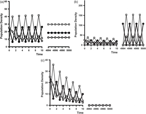This scenario is illustrated in Figure 4.

Figure 4. $\beta =2$, ${\sigma }_1=0.75$, ${\sigma }_2={\sigma }_3=0.50$, $c_{\rho }=20$, $c_2=c_g=0.001$, $w_1=20$, and $w_2=w_3=0$. The open squares are the juvenile class densities. The solid (open) circles are the reproductively active (inactive) adult class densities. Initial conditions are $(x_1,x_2,x_3)=(10,25,25)$. (a) $\rho =90$: In this case $R_0=1.206$ and $c_w=-0.5109\times {10}^{-3}$, $c_b=-0.6068\times {10}^{-4}$, $a_{+}=-0.5716\times {10}^{-4}$, $a_{-}=0.4503\times {10}^{-3}$. (b) $\rho =75$: In this case $R_0=1.107$ and $c_w=-0.4998\times {10}^{-3}$, $c_b=-0.5584\times {10}^{-4}$, $a_{+}=-0.5557\times {10}^{-3}$, $a_{-}=0.4440\times {10}^{-3}$. (c) $\rho =55$: In this case $R_0=0.9320$ and $c_w=-0.4761\times {10}^{-3}$, $c_b=-0.4683\times {10}^{-4}$, $a_{+}=-0.5229\times {10}^{-3}$, $a_{-}=0.4292\times {10}^{-3}$.

On the other hand, when the forward bifurcating synchronous 2-cycles are stable one sees reproductive synchrony arise as the environment deteriorates such that $R_0⪆1$. This is illustrated in Figure 5(b). Figure 5(a) illustrates that the bifurcation results of Theorems 2 and 3 and Corollaries 1 and 2 are, in general, valid only is a neighbourhood of the bifurcation point $(R_0,\overline{x})=(1,\overline{0})$. For the larger value of $R_0>1$ in Figure 5(a) the attractor is a positive equilibrium. Numerical simulation evidence in this example, indicates that the following bifurcation sequence occurs as $R_0$ increases through 1. The extinction equilibrium destabilizes as $R_0$ increases through 1, giving rise to stable synchronous 2-cycles, as shown in Figure  5( c) and 5(b). The synchronous 2-cycles destabilize as $R_0$ is further increased, a bifurcation that gives rise to a branch of stable positive 2-cycles (not shown in Figure 5). These positive 2-cycles are not technical synchronous cycles, but do exhibit oscillations in which the two adult classes are out-of-phase. With further increase in $R_0$ the positive 2-cycles undergo a reverse periodic doubling bifurcation which gives rise to stable positive equilibria, an example of which appears in Figure 5(a). The theorems and corollaries in Section 3 do not cover these secondary bifurcations away from a neighbourhood of $(R_0,\overline{x})=(1,\overline{0})$.

Figure 5. The same parameters as in Figure 4 except $c_g=1$. The open squares are the juvenile class densities. The solid (open) circles are the reproductively active (inactive) adult class densities. Initial conditions are $(x_1,x_2,x_3)=(10,25,25)$. (a) $\rho =90$: In this case $R_0=1.206$ and $c_w=-0.5109\times {10}^{-3}$, $c_b=-0.6068\times {10}^{-1}$, $a_{+}=-0.6119\times {10}^{-1}$, $a_{-}=0.6017\times {10}^{-1}$. (b) $\rho =75$: In this case $R_0=1.107$ and $c_w=-0.4998\times {10}^{-3}$, $c_b=-0.5584\times {10}^{-1}$, $a_{+}=-0.5634\times {10}^{-1}$, $a_{-}=0.5534\times {10}^{-1}$. (c) $\rho =55$: In this case $R_0=0.9320$ and $c_w=-0.4761\times {10}^{-3}$, $c_b=-0.4683\times {10}^{-1}$, $a_{+}=-0.4731\times {10}^{-1}$, $a_{-}=0.4636\times {10}^{-1}$.

4.2.3. A cannibalistic population in a deteriorating environment

A cannibalistic population subjected to the same deteriorating environment can exhibit the same sequence of dynamic changes as that of a non-cannibalistic population as illustrated in Figures 4 and 5 in Section 4.2.2. An example appears in Figure 6.

Figure 6. Sample orbits of model (2(2) $\overline{x}(t+1)=P\left(\overline{x}\right(t\left)\right)\overline{x}\left(t\right),$(2) ) with (16(16) $\begin{array}{rl}b& =\beta u\left(\rho \right),s_i={\sigma }_{i}u\left(\rho \right),\\ \beta & >0,0<{\sigma }_i<1,\end{array}$(16) )–(19(19a) $\begin{array}{r}{p}_{23}\left(\overline{x}\right)=\frac{1}{1+c_g{x}_2}{\beta }_3\left(\frac{1}{1+w_1{x}_1}\frac{w_3(1-u(\rho \left)\right)}{1+w_3(1-u(\rho \left)\right)x_3}{x}_1\right),\end{array}$(19a) ) and parameter values $\beta =2$, ${\sigma }_1=0.75$, ${\sigma }_2={\sigma }_3=0.50$, $c_{\rho }=20$, $c_2=0.001$, $c_g=1$, $w_1=20$, $w_2=w_3=5$, ${\sigma }_{2m}={\sigma }_{3m}=0.95$, $c_{\beta 2}=c_{\beta 3}=1$. The open squares are the juvenile class densities. The solid (open) circles are the reproductively active (inactive) adult class densities. Initial conditions are $(x_1,x_2,x_3)=(10,25,25)$. (a) $\rho =90$: In this case $R_0=1.206$ and $c_w=-0.7652\times {10}^{-1}$, $c_b=-0.4112$, $a_{+}=-0.4877$, $a_{-}=0.3346$. (b) $\rho =75$: In this case $R_0=1.107$ and $c_w=-0.8358\times {10}^{-1}$, $c_b=-0.4574$, $a_{+}=-0.5410$, $a_{-}=0.3738$. (c) $\rho =55$: In this case $R_0=0.9320$ and $c_w=-0.9357\times {10}^{-1}$, $c_b=-0.5419$, $a_{+}=-0.6355$, $a_{-}=0.4484$.

On the other hand, it is possible for a cannibalistic population to undergo backward bifurcations at $R_0=1$ when the benefit to adult survival of cannibalistic resources is significant. In this case, as discussed in Remark 3, there is the potential of a strong Allee effect for values of $R_0<1$. This means that, for a cannibalistic population, survival is possible for some values of $R_0⪅1$. An illustration of this is seen in Figure 7. A comparison of this example with that in Figure 5 for a non-cannibalistic population shows the cannibalistic population surviving in a deteriorated environment ($R_0<1$) when the non-cannibalistic population goes extinct.

Figure 7. Sample orbits of model (2(2) $\overline{x}(t+1)=P\left(\overline{x}\right(t\left)\right)\overline{x}\left(t\right),$(2) ) with (16(16) $\begin{array}{rl}b& =\beta u\left(\rho \right),s_i={\sigma }_{i}u\left(\rho \right),\\ \beta & >0,0<{\sigma }_i<1,\end{array}$(16) )–(19(19a) $\begin{array}{r}{p}_{23}\left(\overline{x}\right)=\frac{1}{1+c_g{x}_2}{\beta }_3\left(\frac{1}{1+w_1{x}_1}\frac{w_3(1-u(\rho \left)\right)}{1+w_3(1-u(\rho \left)\right)x_3}{x}_1\right),\end{array}$(19a) ) and the same parameter values as in Figure 6 except now $c_{\beta 2}=c_{\beta 3}=300$. The open squares are the juvenile class densities. The solid (open) circles are the reproductively active (inactive) adult class densities. Initial conditions are $(x_1,x_2,x_3)=(10,25,25)$. (a) $\rho =90$: In this case $R_0=1.206$ and $c_w=34.01$, $c_b=33.68$, $a_{+}=67.69$, $a_{-}=0.3346$. (b) $\rho =75$: In this case $R_0=1.107$ and $c_w=37.28$, $c_b=36.80$, $a_{+}=73.98$, $a_{-}=0.3738$. (c) $\rho =55$: In this case $R_0=0.9320$ and $c_w=41.66$, $c_b=41.21$, $a_{+}=82.87$, $a_{-}=0.4484$.

5. Concluding remarks

We characterized the unusual bifurcation that occurs in the juvenile–adult model (2(2) $\overline{x}(t+1)=P\left(\overline{x}\right(t\left)\right)\overline{x}\left(t\right),$(2) ) with the imprimitive projection matrix (9(9) $P\left(\overline{x}\right)=\left(\begin{array}{ccc}0& R_0\frac{1-s_2{s}_3}{s_1}{p}_{12}\left(\overline{x}\right)& 0\\ s_1{p}_{21}\left(\overline{x}\right)& 0& s_3{p}_{23}\left(\overline{x}\right)\\ 0& s_2{p}_{32}\left(\overline{x}\right)& s_3{p}_{33}\left(\overline{x}\right)\end{array}\right)$(9) ) that occurs as the extinction equilibrium destabilizes when $R_0$ increases through 1. The two bifurcating continua of equilibria and of synchronous 2-cycles represent quite different dynamic predictions: one of equilibration in which all stages are present at all points in time (i.e. reproductive synchrony is absent) and the other when the adult classes are alternately empty temporally (i.e. reproductive synchrony occurs). By means of the diagnostic quantities $c_b$, $c_w$ and $a_{\pm }$ we determined which of the two alternative dynamics is stable/unstable and what their direction of bifurcations are. These results are summarized in Table 1. These quantities are weighted sums of the sensitivities of the projection matrix entries and allow for biological interpretations of the results in Table 1. The specific models considered in Section 4 provide illustrations. Among the conclusions implied by these particular models are the following.

Table 1. The direction of bifurcation and the stability properties of the bifurcating continua of positive equilibria and synchronous 2-cycles are determined by the signs of the quantities (10) and (11).

Positive equilibria
	$a_{+}>0$	$a_{+}<0$
Direction of bifurcation	Backward	Forward
Stability property	Unstable	Stable if $a_{-}<0$
		Unstable if $a_{-}>0$
Synchronous 2-cycles
	$c_w>0$	$c_w<0$
Direction of bifurcation	Backward	Forward
Stability property	Unstable	Stable if $a_{-}>0$
		Unstable if $a_{-}<0$

1. A non-cannibalistic population will go extinct in a severely deteriorated environment, that is, when $R_0<1$. This is predicted by the model because in the absence of cannibalism the bifurcation at $R_0=1$ is forward.

2. Cannibalism, if sufficiently aggressive, can result in reproductive synchrony. This is mathematically predicted by the dynamic dichotomy of forward bifurcations in Table 1 (right-hand column).

3. A sufficient adult survival benefit from cannibalism can provide for survival when $R_0<1$. This is due to the occurrence of a backward bifurcation (of either the positive equilibria or the synchronous 2-cycles or both) and a resulting strong Allee effect (which means, of course, that survival is initial condition dependent).

To relate a dynamic model more closely to the gull population dynamics that motivated our study, more significant mathematical complications would need to be introduced. For example, the reproductive cycling in our model is that of the maturation period of juveniles. For gulls however the cycling is in days and the maturation period is in years. A model that allows for this difference in time scales is given in [19].

Another issue to be addressed is the evolutionary adaptability of cannibalism and reproductive synchrony. One way to address this question would be to construct and study an evolutionary game theoretic version of (2(2) $\overline{x}(t+1)=P\left(\overline{x}\right(t\left)\right)\overline{x}\left(t\right),$(2) ) with the projection matrix (9(9) $P\left(\overline{x}\right)=\left(\begin{array}{ccc}0& R_0\frac{1-s_2{s}_3}{s_1}{p}_{12}\left(\overline{x}\right)& 0\\ s_1{p}_{21}\left(\overline{x}\right)& 0& s_3{p}_{23}\left(\overline{x}\right)\\ 0& s_2{p}_{32}\left(\overline{x}\right)& s_3{p}_{33}\left(\overline{x}\right)\end{array}\right)$(9) ), along the lines done in [11] for a simpler cannibalism model.

Acknowledgments

The authors gratefully acknowledge the input and significant contributions of Professors James Hayward (Department of Biology, Andrews University) and Shandelle Henson (Department of Mathematics, Andrews University).

Disclosure statement

No potential conflict of interest was reported by the authors.

Notes

1. Solve Equations (3a) and (3c) for $x_1$ and $x_3$ in terms of $x_2$ and substitute the answers into Equation (3b). The result is a quadratic polynomial equation to solve for $x_2$. This quadratic has a positive root (and it is unique) if and only if $R_0>1$.

Appendix 1. Proof of Theorem 2

Part (a) follows from general bifurcation results for matrix models [3]. To prove part (b) we apply the linearization principle. Towards this end, we consider the Jacobian of the map (2(2) $\overline{x}(t+1)=P\left(\overline{x}\right(t\left)\right)\overline{x}\left(t\right),$(2) ) evaluated at the equilibrium (12(12) $\begin{array}{r}{R}_0\left(\epsilon \right)=1-\frac{1}{1-s_2{s}_3}{a}_{+}\epsilon +O\left({\epsilon }^2\right)\end{array}$(12) )–(13(13) $\begin{array}{r}\overline{x}\left(\epsilon \right)={\overline{v}}_{+}\epsilon +O\left({\epsilon }^2\right)\end{array}$(13) ), which we denote by $J\left(\epsilon \right)$. Since $J\left(0\right)=P\left(0\right)$, the three eigenvalues $\lambda \left(\epsilon \right)$ of $J\left(0\right)$ equal 0 and $\pm 1$ when $\epsilon =0$. Thus, one of the eigenvalues of $J\left(\epsilon \right)$ is near 0 for $\epsilon$ small and the stability (by linearization) of the equilibria for $\epsilon$ small depends on the two eigenvalues ${\lambda }_{\pm }\left(\epsilon \right)=\pm 1+{\lambda }_{\pm }^{\mathrm{\prime }}\left(0\right)\epsilon +O\left({\epsilon }^2\right)$ and whether or not they are less than 1 in absolute value for $\epsilon ⪆0$. This is determined by the sign of the $\epsilon$-derivatives ${\lambda }_{\pm }^{\mathrm{\prime }}\left(0\right)$. Let ${\overline{v}}_{\pm }\left(\epsilon \right)$ denote (right) eigenvectors of $J\left(\epsilon \right)$ associated with ${\lambda }_{\pm }\left(\epsilon \right)$: (A1) $J\left(\epsilon \right){\overline{v}}_{\pm }\left(\epsilon \right)={\lambda }_{\pm }\left(\epsilon \right){\overline{v}}_{\pm }\left(\epsilon \right).$(A1) The right and left eigenvectors of $P\left(0\right)$ associated with eigenvalues $\pm 1$ are ${\overline{v}}_{\pm }=\left(\begin{array}{c}1-s_2{s}_3\\ \pm s_1\\ s_1{s}_2\end{array}\right),{\overline{w}}_{\pm }=(s_1\pm 1s_3).$ From Equation (A1(A1) $J\left(\epsilon \right){\overline{v}}_{\pm }\left(\epsilon \right)={\lambda }_{\pm }\left(\epsilon \right){\overline{v}}_{\pm }\left(\epsilon \right).$(A1) ) with $\epsilon =0$ we obtain ${\overline{v}}_{\pm }\left(0\right)={\overline{v}}_{\pm }$. After a differentiation of Equation (A1(A1) $J\left(\epsilon \right){\overline{v}}_{\pm }\left(\epsilon \right)={\lambda }_{\pm }\left(\epsilon \right){\overline{v}}_{\pm }\left(\epsilon \right).$(A1) ) with respect to $\epsilon$ followed by an evaluation at $\epsilon =0$ we have $J\left(0\right){\overline{v}}_{\pm }^{\mathrm{\prime }}\left(0\right)-{\lambda }_{\pm }\left(0\right){\overline{v}}_{\pm }^{\mathrm{\prime }}\left(0\right)={\lambda }_{\pm }^{\mathrm{\prime }}\left(0\right){\overline{v}}_{\pm }-J^{\mathrm{\prime }}\left(0\right){\overline{v}}_{\pm },$ which, by the Fredholm alternative implies ${\overline{w}}_{\pm }\left({\lambda }_{\pm }^{\mathrm{\prime }}\right(0){\overline{v}}_{\pm }-J^{\mathrm{\prime }}(0\left){\overline{v}}_{\pm }\right)=0$ or (A2) ${\lambda }_{\pm }^{\mathrm{\prime }}\left(0\right)=\frac{{\overline{w}}_{\pm }{J}^{\mathrm{\prime }}\left(0\right){\overline{v}}_{\pm }}{{\overline{w}}_{\pm }{\overline{v}}_{\pm }}=\frac{1}{2s_1}{\overline{w}}_{\pm }{J}^{\mathrm{\prime }}\left(0\right){\overline{v}}_{\pm }.$(A2) The Jacobian $J\left(\overline{x}\right)$ of the map $P\left(\overline{x}\right)\overline{x}=\left(\begin{array}{c}{R}_0\frac{1-s_2{s}_3}{s_1}{p}_{12}(x_1,x_2,x_3)x_2\\ s_1{p}_{21}(x_1,x_2,x_3)x_1+s_3{p}_{23}(x_1,x_2,x_3)x_3\\ s_2{p}_{32}(x_1,x_2,x_3)x_2+s_3{p}_{33}(x_1,x_2,x_3)x_3\end{array}\right)$ is $\begin{array}{rl}& \left(\begin{array}{ccc}{R}_0\frac{1-s_2{s}_3}{s_1}{x}_2{\mathrm{\partial }}_1{p}_{12}\left(\overline{x}\right)& R_0\frac{1-s_2{s}_3}{s_1}{x}_2{\mathrm{\partial }}_2{p}_{12}\left(\overline{x}\right)& R_0\frac{1-s_2{s}_3}{s_1}{x}_2{\mathrm{\partial }}_3{p}_{12}\left(\overline{x}\right)\\ s_1{x}_1{\mathrm{\partial }}_1{p}_{21}\left(\overline{x}\right)+s_3{x}_3{\mathrm{\partial }}_1{p}_{23}\left(\overline{x}\right)& s_1{x}_1{\mathrm{\partial }}_2{p}_{21}\left(\overline{x}\right)+s_3{x}_3{\mathrm{\partial }}_2{p}_{23}\left(\overline{x}\right)& s_1{x}_1{\mathrm{\partial }}_3{p}_{21}\left(\overline{x}\right)+s_3{x}_3{\mathrm{\partial }}_3{p}_{23}\left(\overline{x}\right)\\ s_2{x}_2{\mathrm{\partial }}_1{p}_{32}\left(\overline{x}\right)+s_3{x}_3{\mathrm{\partial }}_1{p}_{33}\left(\overline{x}\right)& s_2{x}_2{\mathrm{\partial }}_2{p}_{32}\left(\overline{x}\right)+s_3{x}_3{\mathrm{\partial }}_2{p}_{33}\left(\overline{x}\right)& s_2{x}_2{\mathrm{\partial }}_3{p}_{32}\left(\overline{x}\right)+s_3{x}_3{\mathrm{\partial }}_3{p}_{33}\left(\overline{x}\right)\end{array}\right)\\ & +\left(\begin{array}{ccc}0& R_0\frac{1-s_2{s}_3}{s_1}{p}_{12}\left(\overline{x}\right)& 0\\ s_1{p}_{21}\left(\overline{x}\right)& 0& s_3{p}_{23}\left(\overline{x}\right)\\ 0& s_2{p}_{32}\left(\overline{x}\right)& s_3{p}_{33}\left(\overline{x}\right)\end{array}\right)\end{array}$ which, when evaluated at the equilibrium (12(12) $\begin{array}{r}{R}_0\left(\epsilon \right)=1-\frac{1}{1-s_2{s}_3}{a}_{+}\epsilon +O\left({\epsilon }^2\right)\end{array}$(12) )–(13(13) $\begin{array}{r}\overline{x}\left(\epsilon \right)={\overline{v}}_{+}\epsilon +O\left({\epsilon }^2\right)\end{array}$(13) ), gives $J\left(\epsilon \right)\circeq J\left(\overline{x}\right(\epsilon \left)\right)$. A differentiation of the entries of these matrices followed by an evaluation at $\epsilon =0$ yields $\begin{array}{rl}{J}^{\mathrm{\prime }}\left(0\right)& =\left(\begin{array}{ccc}(1-s_2{s}_3){\mathrm{\partial }}_1^0{p}_{12}& (1-s_2{s}_3){\mathrm{\partial }}_2^0{p}_{12}& (1-s_2{s}_3){\mathrm{\partial }}_3^0{p}_{12}\\ \begin{array}{c}{s}_1(1-s_2{s}_3){\mathrm{\partial }}_1^0{p}_{21}\\ +s_3{s}_1{s}_2{\mathrm{\partial }}_1^0{p}_{23}\end{array}& \begin{array}{c}{s}_1(1-s_2{s}_3){\mathrm{\partial }}_2^0{p}_{21}\\ +s_3{s}_1{s}_2{\mathrm{\partial }}_2^0{p}_{23}\end{array}& \begin{array}{c}{s}_1(1-s_2{s}_3){\mathrm{\partial }}_3^0{p}_{21}\\ +s_3{s}_1{s}_2{\mathrm{\partial }}_3^0{p}_{23}\end{array}\\ s_2{s}_1{\mathrm{\partial }}_1^0{p}_{32}& s_2{s}_1{\mathrm{\partial }}_2^0{p}_{32}+s_3{s}_1{s}_2{\mathrm{\partial }}_2^0{p}_{33}& s_2{s}_1{\mathrm{\partial }}_3^0{p}_{32}\end{array}\right)\\ & +\left(\begin{array}{ccc}0& \frac{1-s_2{s}_3}{s_1}{D}_{{\overline{v}}_{+}}^0{p}_{12}+{\kappa }_1\frac{1-s_2{s}_3}{s_1}& 0\\ s_1{D}_{v_{+}}^0{p}_{21}& 0& s_3{D}_{{\overline{v}}_{+}}^0{p}_{23}\\ 0& s_2{D}_{{\overline{v}}_{+}}^0{p}_{32}& s_1{s}_3{\mathrm{\partial }}_2^0{p}_{33}\end{array}\right).\end{array}$ Here we have used ${\mathrm{\partial }}_1^0{p}_{33}={\mathrm{\partial }}_3^0{p}_{33}=0$ by H2. Using this matrix in Equation (A2(A2) ${\lambda }_{\pm }^{\mathrm{\prime }}\left(0\right)=\frac{{\overline{w}}_{\pm }{J}^{\mathrm{\prime }}\left(0\right){\overline{v}}_{\pm }}{{\overline{w}}_{\pm }{\overline{v}}_{\pm }}=\frac{1}{2s_1}{\overline{w}}_{\pm }{J}^{\mathrm{\prime }}\left(0\right){\overline{v}}_{\pm }.$(A2) ) yields $\begin{array}{rl}{\lambda }_{+}^{\mathrm{\prime }}\left(0\right)& =\frac{1}{2}(1-s_2{s}_3)(c_w+c_b)\\ {\lambda }_{-}^{\mathrm{\prime }}\left(0\right)& =-\frac{1}{2}(c_w-c_b)\end{array}$ and hence $\begin{array}{rl}{\lambda }_{+}\left(\epsilon \right)& =1+\frac{1}{2}(1-s_2{s}_3)(c_w+c_b)\epsilon +O\left({\epsilon }^2\right)\\ {\lambda }_{-}\left(\epsilon \right)& =-1-\frac{1}{2}(c_w-c_b)\epsilon +O\left({\epsilon }^2\right).\end{array}$ A consideration of the signs of ${\lambda }_{\pm }^{\mathrm{\prime }}\left(0\right)$ yields the stability conclusions of part (b).

Appendix 2. Proof of Theorem 3

Part (a). Denote $p_{ij}\left(\overline{x}\right)=p_{ij}(x_1,x_2,x_3)$. From the composite map $\begin{array}{rl}\left(\begin{array}{c}0\\ x_2\\ 0\end{array}\right)& \to \left(\begin{array}{c}{R}_0\frac{1-s_2{s}_3}{s_1}{p}_{12}(0,x_2,0)x_2\\ 0\\ s_2{p}_{32}(0,x_2,0)x_2\end{array}\right)\\ & \to \left(\begin{array}{c}0\\ s_1{p}_{21}\left(R_0\frac{1-s_2{s}_3}{s_1}{p}_{12}(0,x_2,0)x_2,0,s_2{p}_{32}(0,x_2,0)x_2\right)R_0\frac{1-s_2{s}_3}{s_1}{p}_{12}(0,x_2,0)x_2\\ +s_3{p}_{23}\left(R_0\frac{1-s_2{s}_3}{s_1}{p}_{12}(0,x_2,0)x_2,0,s_2{p}_{32}(0,x_2,0)x_2\right)s_2{p}_{32}(0,x_2,0)x_2\\ 0\end{array}\right)\end{array}$ we see (after a cancellation of $x_2$) that synchronous 2-cycles are positive fixed points of the equation $\begin{array}{rl}{x}_2& =R_0(1-s_2{s}_3)p_{21}\left(R_0\frac{1-s_2{s}_3}{s_1}{p}_{12}(0,x_2,0)x_2,0,s_2{p}_{32}(0,x_2,0)x_2\right)p_{12}(0,x_2,0)x_2\\ & +s_2{s}_3{p}_{23}\left(R_0\frac{1-s_2{s}_3}{s_1}{p}_{12}(0,x_2,0)x_2,0,s_2{p}_{32}(0,x_2,0)x_2\right)p_{32}(0,x_2,0)x_2,\end{array}$ which can be considered a one dimensional matrix model (2(2) $\overline{x}(t+1)=P\left(\overline{x}\right(t\left)\right)\overline{x}\left(t\right),$(2) ) with the $1\times 1$ projection matrix $\begin{array}{rl}& R_0(1-s_2{s}_3)p_{21}\left(R_0\frac{1-s_2{s}_3}{s_1}{p}_{12}(0,x_2,0)x_2,0,s_2{p}_{32}(0,x_2,0)x_2\right)p_{12}(0,x_2,0)\\ & +s_2{s}_3{p}_{23}\left(R_0\frac{1-s_2{s}_3}{s_1}{p}_{12}(0,x_2,0)x_2,0,s_2{p}_{32}(0,x_2,0)x_2\right)p_{32}(0,x_2,0).\end{array}$ This can be written $R_0(1-s_2{s}_3)+s_2{s}_3+h(R_0,x_2),$ where $h(R_0,x_2)=O\left(x_2\right)$ for small $x_2$. The bifurcation theorem for general matrix models in [3,6] can be applied to this one dimensional matrix model. The result is a bifurcating continuum of positive roots $x_2$ at $R_0=1$ which has the parameterization $R_0\left(\epsilon \right)=1-\frac{1}{1-s_2{s}_3}{c}_w\epsilon ,x_2\left(\epsilon \right)=s_1\epsilon +O\left({\epsilon }^2\right)$ and the parameterization ${\overline{x}}_2\left(\epsilon \right)={\overline{\pi }}_2\epsilon +O\left({\epsilon }^2\right)$ in part (b). The parameterization of the second point of the resulting synchronous 2-cycle is the image ${\overline{x}}_{13}\left(\epsilon \right)=\left(\begin{array}{c}{R}_0\left(\epsilon \right)\frac{1-s_2{s}_3}{s_1}{p}_{12}(0,x_2(\epsilon ),0)x_2\left(\epsilon \right)\\ 0\\ s_2{p}_{32}(0,x_2(\epsilon ),0)x_2\left(\epsilon \right)\end{array}\right)$ of ${\overline{x}}_2\left(\epsilon \right)$. A straightforward differentiation with respect to $\epsilon$ followed by an evaluation at $\epsilon =0$ yields (14(14) $\begin{array}{rl}{R}_0\left(\epsilon \right)& =1-\frac{1}{1-s_2{s}_3}{c}_w\epsilon +O\left({\epsilon }^2\right)\end{array}$(14) )–(15(15) $\begin{array}{rl}{\overline{x}}_i\left(\epsilon \right)& ={\overline{\pi }}_i\epsilon +O\left({\epsilon }^2\right)\end{array}$(15) ).

Part (b). The stability properties of the synchronous 2-cycles (15(15) $\begin{array}{rl}{\overline{x}}_i\left(\epsilon \right)& ={\overline{\pi }}_i\epsilon +O\left({\epsilon }^2\right)\end{array}$(15) ) can be determined from the linearization principle from eigenvalues of the Jacobian of the composite map $\begin{array}{rl}& \left(\begin{array}{c}\frac{1-s_2{s}_3}{s_1}{R}_0{p}_{12}\left(\overline{y}\right(\overline{x}\left)\right)\left(s_1{p}_{21}\right(\overline{x})x_1+s_3{p}_{23}(\overline{x}\left)x_3\right)\\ (1-s_2{s}_3)R_0{p}_{21}\left(\overline{y}\right(\overline{x}\left)\right)p_{12}\left(\overline{x}\right)x_2+s_3{p}_{23}\left(\overline{y}\right(\overline{x}\left)\right)\left(s_2{p}_{32}\right(\overline{x})x_2+s_3{p}_{33}(\overline{x}\left)x_3\right)\\ s_2{p}_{32}\left(\overline{y}\right(\overline{x}\left)\right)\left(s_1{p}_{21}\right(\overline{x})x_1+s_3{p}_{23}(\overline{x}\left)x_3\right)+s_3{p}_{33}\left(\overline{y}\right(\overline{x}\left)\right)\left(s_2{p}_{32}\right(\overline{x})x_2+s_3{p}_{33}(\overline{x}\left)x_3\right)\end{array}\right)\\ & \overline{y}\left(\overline{x}\right)=\left(\begin{array}{c}{R}_0\frac{1-s_2{s}_3}{s_1}{p}_{12}\left(\overline{x}\right)x_2\\ s_1{p}_{21}\left(\overline{x}\right)x_1+s_3{p}_{23}\left(\overline{x}\right)x_3\\ s_2{p}_{32}\left(\overline{x}\right)x_2+s_3{p}_{33}\left(\overline{x}\right)x_3\end{array}\right)\end{array}$ evaluated at either of the 2-cycle points (15(15) $\begin{array}{rl}{\overline{x}}_i\left(\epsilon \right)& ={\overline{\pi }}_i\epsilon +O\left({\epsilon }^2\right)\end{array}$(15) ). Let $M_k\left(\epsilon \right)=\left[a_{ij}^k\right(\epsilon \left)\right],k=1,2$, denote the Jacobian evaluated at the two points of parameterized 2-cycles (14(14) $\begin{array}{rl}{R}_0\left(\epsilon \right)& =1-\frac{1}{1-s_2{s}_3}{c}_w\epsilon +O\left({\epsilon }^2\right)\end{array}$(14) )–(15(15) $\begin{array}{rl}{\overline{x}}_i\left(\epsilon \right)& ={\overline{\pi }}_i\epsilon +O\left({\epsilon }^2\right)\end{array}$(15) ). It is well known that M is the product of the Jacobians obtained from $J\left(\overline{x}\right)$ evaluated at each of the two points on the 2-cycle $M_1\left(\epsilon \right)=J\left({\overline{x}}_{13}\right(\epsilon \left)\right)J\left({\overline{x}}_2\right(\epsilon \left)\right),M_2\left(\epsilon \right)=J\left({\overline{x}}_2\right(\epsilon \left)\right)J\left({\overline{x}}_{13}\right(\epsilon \left)\right)$ and hence these matrices have the same eigenvalues. Furthermore, $M_k\left(0\right)=P^2\left(0\right)$ has eigenvalues 0 and 1 (repeated). The eigenvalue of $M_k\left(\epsilon \right)$ near 0 for small $\epsilon$ has absolute value less than 1 and we turn to the eigenvalues near 1 for $\epsilon$ small in order to determine the stability of the 2-cycle.

We begin by observing that by H2 and because of the zeros that appear in the cycle points (15(15) $\begin{array}{rl}{\overline{x}}_i\left(\epsilon \right)& ={\overline{\pi }}_i\epsilon +O\left({\epsilon }^2\right)\end{array}$(15) ) a straightforward calculation shows that $a_{12}^k\left(\epsilon \right)\equiv a_{32}^k\left(\epsilon \right)\equiv 0$ for all $\epsilon$ and both k=1,2. The composite Jacobian $M_k\left(\epsilon \right)=\left(\begin{array}{ccc}{a}_{11}^k\left(\epsilon \right)& 0& a_{11}^k\left(\epsilon \right)\\ a_{21}^k\left(\epsilon \right)& a_{22}^k\left(\epsilon \right)& a_{23}^k\left(\epsilon \right)\\ a_{31}^k\left(\epsilon \right)& 0& a_{33}^k\left(\epsilon \right)\end{array}\right)$ has eigenvalues $a_{22}^k\left(\epsilon \right)$ for k=1,2. The entry $a_{22}$ in the Jacobian of the composite is ${\mathrm{\partial }}_2\left[\right(1-s_2{s}_3\left)R_0{p}_{21}\right(\overline{y}\left(\overline{x}\right)\left)p_{12}\right(\overline{x})x_2+s_3{p}_{23}(\overline{y}\left(\overline{x}\right)\left)\right(s_2{p}_{32}\left(\overline{x}\right)x_2+s_3{p}_{33}\left(\overline{x}\right)x_3\left)\right],$ which is straightforwardly calculated by means of the product and chain rules. If we carry out this differentiation and evaluate the result at the cycle points ${\overline{x}}_2\left(\epsilon \right)$ and ${\overline{x}}_{13}\left(\epsilon \right)$ we obtain $a_{22}^1\left(\epsilon \right)$ and $a_{22}^2\left(\epsilon \right)$, respectively. It is helpful for this somewhat tedious calculation to keep in mind the appearance of zeros in ${\overline{x}}_2\left(\epsilon \right)$ and ${\overline{x}}_{13}\left(\epsilon \right)$. The results are $\begin{array}{rl}{a}_{22}^1\left(\epsilon \right)& =1+c_w\epsilon +O\left({\epsilon }^2\right),\\ a_{22}^2\left(\epsilon \right)& =1-(c_w-c_b)\epsilon +O\left({\epsilon }^2\right).\end{array}$ For $\epsilon ⪆0$ both eigenvalues are positive and less than 1 if the $\epsilon$-coefficients are negative, and one of these eigenvalues will be greater than 1 if one of the $\epsilon$-coefficients is positive.

References

- H. Caswell, Matrix Population Models: Construction, Analysis and Interpretation, 2nd ed., Sinauer Associates, Inc. Publishers, Sunderland, MA, 2001.
- F. Courchamp, L. Berec, and J. Gascoigne, Allee Effects in Ecology and Conservation, Oxford University Press, Oxford, 2008.
- J.M. Cushing, An Introduction to Structured Population Dynamics, Conference Series in Applied Mathematics, Vol. 71, SIAM, Philadelphia, 1998.
- J.M. Cushing, Nonlinear semelparous Leslie models, Math. Biosci. Eng. 3(1) (2006), pp. 17–36. doi: 10.3934/mbe.2006.3.17
- J.M. Cushing, Three stage semelparous Leslie models, J. Math. Biol. 59 (2009), pp. 75–104. doi: 10.1007/s00285-008-0208-9
- J.M. Cushing, Matrix models and population dynamics, in Mathematical Biology, M.A. Lewis, J. Chaplain, J.P. Keener, and P.K. Maini, eds., IAS/Park City Mathematics Series, American Mathematical Society, Providence, RI, 2009, pp. 47–150.
- J.M. Cushing, Backward bifurcations and strong Allee effects in matrix models for the dynamics of structured populations, J. Biol. Dyn. 8 (2014), pp. 57–73. doi: 10.1080/17513758.2014.899638
- J.M. Cushing, On the fundamental bifurcation theorem for semelparous Leslie models, Chapter 11 in Mathematics of Planet Earth: Dynamics, Games and Science, J.P. Bourguignon, R. Jeltsch, A. Pinto, and M. Viana, eds., CIM Mathematical Sciences Series, Springer, Berlin, 2015, pp. 215–251.
- J.M. Cushing and S.M. Henson, Stable bifurcations in nonlinear semelparous Leslie models, J. Biol. Dyn. 6 (2012), pp. 80–102. doi: 10.1080/17513758.2012.716085
- J.M. Cushing and Z. Yicang, The net reproductive value and stability in structured population models, Natur. Resource Modeling 8(4) (1994), pp. 1–37.
- J.M. Cushing, S.M. Henson, and J.L. Hayward, An evolutionary game theoretic model of cannibalism, Natur. Resource Modeling 28(4) (2015), pp. 497–521. doi: 10.1111/nrm.12079
- F. Darling, Bird Flocks and the Breeding Cycle, Cambridge University Press, Cambridge, 1938.
- Q. Dong and G.A. Polis, The dynamics of cannibalistic populations: A foraging perspective, in Cannibalism: Ecology and Evolution Among Diverse Taxa, M.A. Elgar and B.J. Crespi, eds., Oxford University Press, Oxford, 1992, pp. 13–37.
- S.N. Elaydi, An Introduction to Difference Equations, Springer-Verlag, New York, 1996.
- M.A. Elgar and B.J. Crespi, Cannibalism: Ecology and Evolution Among Diverse Taxa, Oxford University Press, Oxford, 1992.
- L.R. Fox, Cannibalism in natural populations, Annu. Rev. Ecol. Syst. 6 (1975), pp. 87–106. doi: 10.1146/annurev.es.06.110175.000511
- J.L. Hayward, L.M. Weldon, S.M. Henson, L.C. Megna, B.G. Payne, and A.E. Moncrieff, Egg cannibalism in a gull colony increases with sea surface temperature, Condor 116 (2014), pp. 62–73. doi: 10.1650/CONDOR-13-016-R1.1
- S.M. Henson, J.L. Hayward, J.M. Cushing, and J.G. Galusha, Socially induced synchronization of every-other-day egg laying in a seabird colony, Auk 127 (2010), pp. 571–580. doi: 10.1525/auk.2010.09202
- S.M. Henson, J.M. Cushing, and J.L. Hayward, Socially-induced ovulation synchrony and its effect on seabird populations, J. Biol. Dyn. 5 (2011), pp. 495–516. doi: 10.1080/17513758.2010.529168
- R. Kon, Y. Saito, and Y. Takeuchi, Permanence of single-species stage-structured models, J. Math. Biol. 48 (2004), pp. 515–528. doi: 10.1007/s00285-003-0239-1
- C.-K. Li and H. Schneider, Applications of Perron-Frobenius theory to population dynamics, J. Math. Biol. 44 (2002), pp. 450–462. doi: 10.1007/s002850100132
- G.A. Polis, The evolution and dynamics of intraspecific predation, Annu. Rev. Ecol. Syst. 12 (1981), pp. 225–251. doi: 10.1146/annurev.es.12.110181.001301