Modelling populations of Lygus hesperus on cotton fields in the San Joaquin Valley of California: the importance of statistical and mathematical model choice

ABSTRACT

Understanding the population dynamics of herbivorous insects is critical to developing and implementing effective pest control protocols. In the context of inverse problems, we explore the dynamic effects of pesticide treatments on Lygus hesperus, a common pest of cotton in the western United States. Fitting models to field data, we explore the topic of model selection for an appropriate mathematical model and corresponding statistical models, and use techniques including ANOVA-based model comparison tests and residual plot analysis to make the best selections. In addition we explore the topic of data information content: in this example, we are testing the question of whether data, as it is currently collected, can support time-dependent parameter estimation. Furthermore, we investigate the statistical assumptions often haphazardly made in the process of parameter estimation and consider the implications of unfounded assumptions.

KEYWORDS:

• Inverse problem
• ordinary least squares
• generalized least squares
• model selection
• information content
• bootstrapping
• residual plots
• linear splines
• hemiptera
• herbivory
• pest suppression
• pesticide

1. Introduction

It has long been understood that solving problems in applied ecology often relies on an accurate understanding of population dynamics [19, 24]. When addressing questions in fields ranging from conservation science to agricultural production, ecologists often collect time-series data in order to better understand how populations behave when subjected to abiotic or biotic disturbance [11, 12, 29]. Furthermore, in many cases, the development and analysis of mathematical models can help make sense of time-series data as well as predict future population responses to ecological drivers. Fitting models to data, which requires a broad understanding of both statistics and mathematics, is thus an important component of understanding pattern and process in population studies. In agricultural ecology, pesticide disturbance may disrupt predator-prey interactions [35, 36] as well as impose both acute and chronic effects on arthropod populations [17, 26, 39]. In the past two decades, the focus of many studies of pesticide effects on pests and their natural enemies has shifted away from static measures such as the LC${}_{50}$, instead emphasizing population metrics/outcomes [20–22, 34, 37]. In the meantime, we now have decades of field studies that have generated time-series data aimed at assessing the effects of pesticides on arthropods at the population level [10, 23, 27, 30, 33, 35, 41]. When working with real data, one must consider the strength or information content [8] of the data set. This can be described as an understanding of how strongly one can carry out model validation given a particular data set. There are many ways to quantify the content of a data set, including use of sensitivities, the Fisher Information Matrix and Akaike Information Criteria methods [4, 8, 9, 13, 38]. Simple mathematical models, parameterized with field data, are often used to then predict the consequences of increasing or decreasing pesticide exposure in the field. Accuracy in parameter estimation and fitting data to models, which has received increasing attention in ecological circles [25, 28], depends critically on the appropriate model selection. In all cases, this includes optimal selection of both statistical and mathematical models fit to data – something that is not always fully explicitly addressed in the ecological literature. We address this gap using data from pest population counts of Lygus hesperus Knight (Hemiptera: Meridae) feeding on pesticide-treated cotton fields in the San Joaquin Valley of California [31]. In particular, we fit L. hesperus counts to a simple mathematical model and consider two statistical models: one assuming absolute error and one assuming relative error. We carry out model selection between two nested mathematical models, and compare the outcomes when assuming absolute error versus relative error.

2. Methods

2.1. Data

Our database consists of approximately 1500 replicates of L. hesperus density counts, using sweep counts, in over 500 Pima or Acala cotton fields in 2004–2008. In each replicate, data was collected by one of four pest control advisors (PCAs) between June 1 and August 30. Although there was variability in data collection schedule between PCAs and between replicates, fields were sampled roughly 1–3 times per week, at irregular times during these summer months. In addition, some PCAs chose to count both nymph and adult L. hesperus, while others simply counted the total number of L. hesperus caught in the nets. In addition, the replicates varied in the presence or absence of chemical treatments, as well as in frequency, schedule, and variety of pesticide applications, ranging from zero to six applications in one season. However, the netting effort was standardized across all PCAs and all replicates.

Within the entire database, we consider a particular replicate, which we will denote as replicate 1, that was treated with pesticides three times intermittently between 1 June and 30 August 2007. The pesticides (and the associated targets) used on this replicate are summarized in Table 1. Note that in addition to the target types listed, additional chemicals may have been applied, such as surfactants, plant nutrients, and adjuvants. Although it is likely that these chemicals have little effect on L. hesperus, effects are still possible; however, they will be ignored in our analysis.

Table 1. Dates, pesticides, and pests targeted in chemical treatments applied to replicate 1.

Date	Chemical treatments	Targets
June 12	B-85/STEWARD	Beet armyworms
June 21	Prowl H2O/IGNITE	Weeds
	2/B-85/CHATEAU/TRIMAX PRO	Aphids
	1/ZEPHYR 0.15EC	Mites
July 27	HOOK / ZEAL	Mites

2.2. Statistical models

We now describe the statistical model, in terms of the mathematical model and the collected data. Let $\mathbf{\text{x}}$ denote the $N-$dimensional vector of state variables (x for the scalar case), with $\theta \theta =[\mathbf{\text{q}},{\mathbf{\text{x}}}_0]$ (if initial conditions ${\mathbf{\text{x}}}_0$ are unknown) denoting parameters to be estimated in the ordinary differential equation (ODE) system (mathematical model) (1) $\begin{array}{rl}\frac{\mathrm{d}\mathbf{\text{x}}}{\mathrm{d}t}& =\mathbf{\text{g}}(t,\mathbf{\text{x}}(t),\mathbf{\text{q}})\\ \mathbf{\text{x}}\left(t_0\right)& ={\mathbf{\text{x}}}_0.\end{array}$(1) In many cases, not all variables are observed in data collection, so we define the m-dimensional observation process $\mathbf{\text{f}}(t;\theta \theta )=\mathcal{C}\mathbf{\text{x}}(t;\theta \theta )$, with $m\le N$. Assume we have n data points ${\mathbf{\text{y}}}_j$ at discrete time points $\{t_j{\}}_{j=1}^n$. It follows that $\mathbf{\text{f}}(t_j;\theta \theta )=\mathcal{C}\mathbf{\text{x}}(t_j;\theta \theta )$ for $j=1,\dots ,n$.

We now define the statistical model: a quantified relationship between the observed model output and the raw data; similarly, one could think of this as a description of the measurement/observation error. First consider an absolute error model (2) ${\mathbf{\text{Y}}}_j=\mathbf{\text{f}}(t_j,\theta {\theta }_0)+{\mathcal{E}}_j,j=1,\dots ,n,$(2) with realization (3) ${\mathbf{\text{y}}}_j=\mathbf{\text{f}}(t_j,\theta {\theta }_0)+ϵ{ϵ}_j,j=1,\dots ,n,$(3) where $\theta {\theta }_0$ is the $p\times 1$ ‘true’ parameter vector which we assume exists. Observe that $\mathbf{\text{f}}(t_j,\theta {\theta }_0)$ is completely deterministic, so the randomness of the $m\times 1$ vector ${\mathbf{\text{Y}}}_j$ is due to the $m\times 1$-dimensional random error ${\mathcal{E}}_j$ (for $j=1,\dots ,n$). We assume that ${\mathcal{E}}_j,j=1,\dots ,n$ has zero mean and covariance matrix given by $V_0=\mathrm{Var}\left({\mathcal{E}}_j\right)=\mathrm{diag}({\sigma }_1^2,{\sigma }_2^2,\dots ,{\sigma }_m^2)$ for $j=1,\dots ,n$ (where $\{{\sigma }_i^2{\}}_{i=1}^m$ are constants). Error of this kind is often described as i.i.d – independent and identically distributed. Let $\overline{\mathbf{\text{Y}}}$ be the $m\times n$ matrix whose n columns are the $m\times 1$ random vectors $\{{\mathbf{\text{Y}}}_j{\}}_{j=1}^n$; that is, $\overline{\mathbf{\text{Y}}}=[{\mathbf{\text{Y}}}_1,{\mathbf{\text{Y}}}_2,\dots ,{\mathbf{\text{Y}}}_n]$. One seeks to estimate unknown parameters by minimizing the least squares discrepancy between model output and data. In other words, one must minimize the ordinary least squares (OLS) cost functional (4) $J_n(\overline{\mathbf{\text{Y}}},\theta \theta )=\frac{1}{n}\sum _{j=1}^n[{\mathbf{\text{Y}}}_j-\mathbf{\text{f}}(t_j,\theta \theta \left){]}^T\right[{\mathbf{\text{Y}}}_j-\mathbf{\text{f}}(t_j,\theta \theta )].$(4) Because $\{{\mathbf{\text{Y}}}_j{\}}_{j=1}^n$ are random vectors, one must define the estimator $\theta {\theta }_{\mathrm{OLS}}^n=\arg \underset{\theta \theta \in \mathcal{Q}}{min}{J}_n(\overline{\mathbf{\text{Y}}},\theta \theta )$ and corresponding estimate (5) ${\widehat{\theta \theta }}^n:={\widehat{\theta \theta }}_{\mathrm{OLS}}^n=\arg \underset{\theta \theta \in \mathcal{Q}}{min}{J}_n(\overline{\mathbf{\text{y}}},\theta \theta ).$(5) That is, ${\widehat{\theta \theta }}^n$ is the best OLS estimate for $\theta {\theta }_0$.

This absolute error model is often haphazardly and incorrectly assumed in both maximum likelihood and least squares optimization methods. (In choosing an optimization method, one should recall that maximum likelihood models also require an assumption of the underlying error probability model.) The modeler can carefully choose this error model to allow for some type of relative error [2, 4] if such a model can be correctly identified. Thus the modeler should also (in the absence of specific information on the error process) consider a relative error model of the form (6) ${\mathbf{\text{Y}}}_j=\mathbf{\text{f}}(t_j,\theta {\theta }_0)+{\mathbf{\text{f}}}^{\gamma }(t_j,\theta {\theta }_0)\circ {\mathcal{E}}_j,j=1,\dots ,n,$(6) with realization (7) ${\mathbf{\text{y}}}_j=\mathbf{\text{f}}(t_j,\theta {\theta }_0)+{\mathbf{\text{f}}}^{\gamma }(t_j,\theta {\theta }_0)\circ ϵ{ϵ}_j,j=1,\dots ,n,$(7) where γ is some constant that depends on the given data set. Because $\mathbf{\text{f}}$ and ${\mathcal{E}}_j$ are both $m\times 1$-dimensional operators, ‘○’ denotes component-wise multiplication in Equations (6(6) ${\mathbf{\text{Y}}}_j=\mathbf{\text{f}}(t_j,\theta {\theta }_0)+{\mathbf{\text{f}}}^{\gamma }(t_j,\theta {\theta }_0)\circ {\mathcal{E}}_j,j=1,\dots ,n,$(6) ) and (7(7) ${\mathbf{\text{y}}}_j=\mathbf{\text{f}}(t_j,\theta {\theta }_0)+{\mathbf{\text{f}}}^{\gamma }(t_j,\theta {\theta }_0)\circ ϵ{ϵ}_j,j=1,\dots ,n,$(7) ). When $\gamma =0$, Equation (6(6) ${\mathbf{\text{Y}}}_j=\mathbf{\text{f}}(t_j,\theta {\theta }_0)+{\mathbf{\text{f}}}^{\gamma }(t_j,\theta {\theta }_0)\circ {\mathcal{E}}_j,j=1,\dots ,n,$(6) ) is equivalent to Equation (2(2) ${\mathbf{\text{Y}}}_j=\mathbf{\text{f}}(t_j,\theta {\theta }_0)+{\mathcal{E}}_j,j=1,\dots ,n,$(2) ). In the case of population models, Equation (6(6) ${\mathbf{\text{Y}}}_j=\mathbf{\text{f}}(t_j,\theta {\theta }_0)+{\mathbf{\text{f}}}^{\gamma }(t_j,\theta {\theta }_0)\circ {\mathcal{E}}_j,j=1,\dots ,n,$(6) ) is often correct, and represents error with non-constant variance (which may depend on the output function $\mathbf{\text{f}}(t,\theta \theta )$). One can determine if a given statistical model is appropriate by examining residual plots (residuals versus time, residuals versus observed output) and visually determining if they violate the assumption that the residuals are i.i.d. [2]. Typically, this visual investigation is also how one determines the best value of γ. We will consider both statistical models and determine the best choice.

For ease of notation, we will present the remaining methodology in the context of the scalar problem (N=1), although all methodology can be easily extended to vector systems. Therefore, when referring to the random observation variable, we will now use the notation $\mathbf{\text{Y}}=[Y_1,Y_2,\dots ,Y_n]$ where $Y_j$ is the one-dimensional version of the previously defined ${\mathbf{\text{Y}}}_j$.

2.3. Residual plots and generalized least squares

Residual plots are powerful in their ability to illuminate incorrect assumptions regarding observation error. One can examine the residual plots versus time and model output, respectively, and determine whether the scatter of the error seems to violate the statistical assumptions [2]. This simple process can often prevent a crucial mistake – an incorrect statistical model assuming absolute error and other modelling mistakes. If one finds that the relative error statistical model (6(6) ${\mathbf{\text{Y}}}_j=\mathbf{\text{f}}(t_j,\theta {\theta }_0)+{\mathbf{\text{f}}}^{\gamma }(t_j,\theta {\theta }_0)\circ {\mathcal{E}}_j,j=1,\dots ,n,$(6) ) is most suitable, for some γ, one must replace the cost functional (4(4) $J_n(\overline{\mathbf{\text{Y}}},\theta \theta )=\frac{1}{n}\sum _{j=1}^n[{\mathbf{\text{Y}}}_j-\mathbf{\text{f}}(t_j,\theta \theta \left){]}^T\right[{\mathbf{\text{Y}}}_j-\mathbf{\text{f}}(t_j,\theta \theta )].$(4) ) with a generalized least squares (GLS) formulation [2, 4, 14, 16, 32] (8) ${\tilde{J}}_n\left(\mathbf{\text{Y}}\right)=\frac{1}{n}\sum _{j=1}^n{\omega }_j[Y_j-f(t_j,\theta \theta ){]}^2$(8) with weights ${\omega }_j={\omega }_j\left(\theta \theta \right)=f^{-2\gamma }(t_j,\theta \theta )$, $j=1,\dots ,n$. Consequently, one must redefine the estimator $\theta {\theta }_{\mathrm{GLS}}^n=\arg \underset{\theta \theta \in \mathcal{Q}}{min}{\tilde{J}}_n(\mathbf{\text{Y}},\theta \theta )$ with corresponding estimate (9) ${\widehat{\theta \theta }}^n:={\widehat{\theta \theta }}_{\mathrm{GLS}}^n=\arg \underset{\theta \theta \in \mathcal{Q}}{min}{\tilde{J}}_n(\mathbf{\text{y}},\theta \theta ).$(9)

We assume an error model in the form of (8(8) ${\tilde{J}}_n\left(\mathbf{\text{Y}}\right)=\frac{1}{n}\sum _{j=1}^n{\omega }_j[Y_j-f(t_j,\theta \theta ){]}^2$(8) ), but a more generalized form of error model for GLS methods can be found in [3, 4, 14, 16, 32]. GLS estimates ${\widehat{\theta \theta }}^n$ and estimated weights $\left\{{\omega }_j\right(\theta \theta ){\}}_{j=1}^n$ are found using a standard iterative method [2, 4, 14, 16, 32] as given below . For the sake of notation, we will suppress the sample size superscript n (i.e. ${\widehat{\theta \theta }}_{\mathrm{GLS}}:={\widehat{\theta \theta }}_{\mathrm{GLS}}^n$) in describing the iterative method.

1. Estimate ${\widehat{\theta \theta }}_{\mathrm{GLS}}$ by ${\widehat{\theta \theta }}^{\left(0\right)}$ using OLS method (4(4) $J_n(\overline{\mathbf{\text{Y}}},\theta \theta )=\frac{1}{n}\sum _{j=1}^n[{\mathbf{\text{Y}}}_j-\mathbf{\text{f}}(t_j,\theta \theta \left){]}^T\right[{\mathbf{\text{Y}}}_j-\mathbf{\text{f}}(t_j,\theta \theta )].$(4) ). Set k=0.

2. Compute weights ${\hat{\omega }}_j=f^{-2\gamma }(t_j,{\widehat{\theta \theta }}^{\left(k\right)})$.

3. Obtain k+1 estimate for ${\widehat{\theta \theta }}_{\mathrm{GLS}}$ with ${\widehat{\theta \theta }}^{(k+1)}:=\arg min\left(1/n\right)\sum _{j=1}^n{\hat{\omega }}_j[y_j-f(t_j,\theta \theta ){]}^2$.

4. Set k:=k+1 and return to step 2. Terminate when the two successive estimates for ${\widehat{\theta \theta }}_{\mathrm{GLS}}$ are sufficiently close.

2.4. Mathematical models

In previous modelling attempts of L. hesperus population in untreated fields, an exponential model adequately described the total population growth [9]. However, manipulations of the system, such as pesticide applications, time-varying presence of predators or prey, or resource changes, can be mathematically represented with time-varying parameters. We now consider a modified model incorporating time-dependent growth due to chemical applications. Let $j^{\ast }$= the number of pesticide applications in a data set. Let model A be as follows: (10) $\begin{array}{rl}\frac{\mathrm{d}x}{\mathrm{d}t}& =k\left(t\right)x,\\ x\left(t_1\right)& =x_1,\end{array}$(10) where $t_1$ is the time of the first data point, and $k\left(t\right)$ is a time dependent growth rate $k\left(t\right)=\left\{\begin{array}{ll}\eta +p\left(t\right)& t\in P_j,j\in \{1,2,3\},\\ \eta & \mathrm{otherwise},\end{array}\right.$ where $p\left(t\right)$ is described below, and $P_j=[t_{p_j},t_{p_j}+1/4],j=1,\dots j^{\ast }$ with $t_{p_j}$ as the time point of the jth pesticide application. Note that $|P_j|=1/4$ which is approximately the length of time of one week when t is measured in months. This reflects the general assumption that pesticides and herbicides are most active during the 7 days immediately following treatment. Clearly, η is the constant growth rate of the total population in the absence of pesticides. In addition, t=0 refers to June 1 (as no data are present before June 1 in our database).

We use linear splines to approximate $p\left(t\right)$ as follows. Consider m linear splines: $p\left(t\right)=\sum _{i=1}^s{\lambda }_i{l}_i\left(t\right),$ where (11) $l_i\left(t\right)=1/h\left\{\begin{array}{ll}t-{\overline{t}}_{i-1}& {\overline{t}}_{i-1}\le t<{\overline{t}}_i,\\ {\overline{t}}_{i+1}-t& {\overline{t}}_i\le t\le {\overline{t}}_{i+1},\\ 0& \mathrm{otherwise},\end{array}\right.$(11) where the evenly spaced spline functions are centred over nodes $\left\{{\overline{t}}_i\right\}$ given by $t_{p_j}:|P_j|/(s+1):t_{p_j}+1/4$, and the step size h is given by $h={\overline{t}}_i-{\overline{t}}_{i-1}$. For our analysis with this model, to impose continuity of $k\left(t\right)$, we do not include the splines centred over the ‘end’ nodes, that is, $t=t_{p_j}$, and $t=t_{p_j}+1/4$. Linear spline approximations are simple, yet flexible in that they allow the modeler to avoid assuming a certain shape to the curve being approximated. Incorporating a time-dependent parameter such as $k\left(t\right)$ is useful when modelling a system with discontinuous perturbations (such as the removal of a predator, or the application of an insecticide). The addition of more splines (s>3) provides a finer approximation, but demands more terms in the parameter estimates. We conjecture that it is likely that s=3 (excluding splines centred at interval endpoints) is sufficient. An example of three linear splines over the interval [0, 0.25 ] is given in Figure 1(a). A sample function $p\left(t\right)$ for some chosen values of $\{{\lambda }_i{\}}_{i=1}^3$ is pictured in Figure 1(b). Now consider model B: (12) $\begin{array}{rl}\frac{\mathrm{d}x}{\mathrm{d}t}& =\eta x,\\ x\left(t_1\right)& =x_1,\end{array}$(12) where $x_1,\eta$ are defined as above. Note that model B is equivalent to model A when applying the constraint $p\left(t\right)\equiv 0$, that is, ${\lambda }_i=0$ for i=1,2,3. Therefore, this is the case of comparing nested models, and an ANOVA model comparison test is applicable to determine whether a time-dependent growth parameter is not only appropriate in describing these population dynamics, but can also be estimated given the information content of the data. In our analysis of models A and B, we first estimated the initial condition $x_1$ using model B (as this data point precedes any pesticide applications and provides a better estimate for $x_1$), and then fixed this parameter in all subsequent parameter estimates. Therefore, the parameters to be estimated are $\theta \theta =\mathbf{\text{q}}=[\eta ,{\lambda }_1,{\lambda }_2,{\lambda }_3{]}^T$.

Figure 1. (a) An example of three linear splines centred over evenly spaced nodes over the interval [0, 0.25 ], not including splines centred at the endpoints where $p\left(t\right)$ must be zero, as defined in Equation (11(11) $l_i\left(t\right)=1/h\left\{\begin{array}{ll}t-{\overline{t}}_{i-1}& {\overline{t}}_{i-1}\le t<{\overline{t}}_i,\\ {\overline{t}}_{i+1}-t& {\overline{t}}_i\le t\le {\overline{t}}_{i+1},\\ 0& \mathrm{otherwise},\end{array}\right.$(11) ), and (b) an example of $p\left(t\right)$ over the interval [0, 0.25 ] with spline sum coefficients $\{{\lambda }_i{\}}_{i=1}^3=\{-8,-9,-5\}$.

2.5. Model comparison test

We now present the residual sum of squares ANOVA-type model comparison test based on confidence levels [14, 16, 32] as developed in [1], described in detail in [2, 4] and extended in [5] to GLS problems. This test is used to determine which of several nested models is the best fit to the data; therefore, this test can be applied to the comparison of models A and B. While Akaike Information Criteria methods are commonly known to incorporate both model fit and model complexity into quantifying a model selection score [38], this ANOVA-based model comparison test for nested models indirectly incorporates the number of model parameters into the resulting test statistic, as will be seen below. Again, for ease of notation and because we are applying this test to the comparison of one-dimensional models, we will present everything in the scalar case (although it can be applied to a general vector system).

Assume we have math model $f(t,\theta \theta )$ and n observations $\mathbf{\text{Y}}=\{Y_j{\}}_{j=1}^n$ with realizations $\mathbf{\text{y}}=\{y_j{\}}_{j=1}^n$ and assume the statistical model assumes either absolute or relative error and takes the form of (2(2) ${\mathbf{\text{Y}}}_j=\mathbf{\text{f}}(t_j,\theta {\theta }_0)+{\mathcal{E}}_j,j=1,\dots ,n,$(2) ) or (6(6) ${\mathbf{\text{Y}}}_j=\mathbf{\text{f}}(t_j,\theta {\theta }_0)+{\mathbf{\text{f}}}^{\gamma }(t_j,\theta {\theta }_0)\circ {\mathcal{E}}_j,j=1,\dots ,n,$(6) ), respectively. Here we will describe the methodology in the context of absolute error (OLS optimization), but this test can be readily extended in the case of relative error and GLS optimization [4, 5].

Let $\mathcal{Q}$ denote the admissible parameter set, where $\mathcal{Q}$ is a compact subset of ${\mathbb{R}}^p$, with $\theta {\theta }_0\in \mathrm{int}\left(\mathcal{Q}\right)$. Recall that we define the OLS estimator ${\displaystyle \theta {\theta }_{\mathrm{OLS}}^n=\arg \underset{\theta \theta \in \mathcal{Q}}{min}{J}_n(\mathbf{\text{Y}},\theta \theta )}$ with corresponding estimate ${\widehat{\theta \theta }}^n:={\widehat{\theta \theta }}_{\mathrm{OLS}}^n=\arg \underset{\theta \theta \in \mathcal{Q}}{min}{J}_n(\mathbf{\text{y}},\theta \theta ).$ It is useful to test if $\theta \theta \in {\mathcal{Q}}_H$, where ${\mathcal{Q}}_H$ is some particular subset of $\mathcal{Q}$ of the form (13) ${\mathcal{Q}}_H=\{\theta \theta \in \mathcal{Q}|H\theta \theta =\mathbf{\text{c}}\},$(13) where H is an $r\times p$ matrix of full rank, and $\mathbf{\text{c}}$ is an $r\times 1$ constant vector, whose entries are determined by the problem at hand. We can formulate the null and alternative hypotheses:

• H${}_0$: The fit provided by model A does not provide a statistically significantly better fit to the data than the fit provided by model B.

• H${}_A$: The fit provided by model A does provide a statistically significantly better fit to the data than the fit provided by model B.

In other words, the null hypothesis H${}_0$ is equivalent to the statement $\theta {\theta }_0\in {\mathcal{Q}}_H$. If we define $\theta {\theta }_H^n\left(\mathbf{\text{Y}}\right)=\arg \underset{\theta \theta \in {\mathcal{Q}}_H}{min}{J}_n(\mathbf{\text{Y}},\theta \theta ),{\widehat{\theta \theta }}_H^n\left(\mathbf{\text{ y}}\right)=\arg \underset{\theta \theta \in {\mathcal{Q}}_H}{min}{J}_n(\mathbf{\text{y}},\theta \theta )$ we notice that $J_n(\mathbf{\text{y}},{\widehat{\theta \theta }}_H^n)\ge J_n(\mathbf{\text{y}},{\widehat{\theta \theta }}^n)$. Next, we define the non-negative test statistic and realization by $T_n\left(\mathbf{\text{Y}}\right)=n\left(J_n\right(\mathbf{\text{Y}},\theta {\theta }_H^n)-J_n(\mathbf{\text{Y}},\theta {\theta }^n\left)\right),{\hat{T}}_n\left(\mathbf{\text{y}}\right)=n\left(J_n\right(\mathbf{\text{ y}},{\widehat{\theta \theta }}_H^n)-J_n(\mathbf{\text{y}},{\widehat{\theta \theta }}^n\left)\right).$ We then define the test statistic and realization $U_n\left(\mathbf{\text{Y}}\right)=\frac{T_n\left(\mathbf{\text{Y}}\right)}{J_n(\mathbf{\text{Y}},\theta {\theta }^n)},{\hat{U}}_n\left(\mathbf{\text{y}}\right)=\frac{T_n\left(\mathbf{\text{ y}}\right)}{J_n(\mathbf{\text{y}},{\widehat{\theta \theta }}^n)}.$ Under certain assumptions (see [1, 4] for details), we have the following conclusions:

1. $\theta {\theta }^n\to \theta {\theta }_0$ with probability one as $n\to \mathrm{\infty }$;

2. If H${}_0$ is true, $U_n\to U$ in distribution as $n\to \mathrm{\infty }$, where $U\sim {\chi }^2\left(r\right)$, a ${\chi }^2$ distribution with r degrees of freedom with r being the number of constraints on the parameter space ${\mathcal{Q}}_H$, as defined in Equation (13(13) ${\mathcal{Q}}_H=\{\theta \theta \in \mathcal{Q}|H\theta \theta =\mathbf{\text{c}}\},$(13) ).

Now consider two parameters of interest: a threshold τ and significance level α, where for a given τ, $\alpha =\mathrm{Prob}(U>\tau )$. This statistic relates to our null hypothesis in the following way: $\begin{array}{rl}& \mathbf{\text{If the test statistic}}{\hat{U}}_n>\tau ,{\mathbf{\text{we reject H}}}_0\mathbf{\text{as false with confidence level}}\\ & (1-\alpha )\times 100\mathrm{\%}.{\mathbf{\text{Otherwise, we do not reject H}}}_0.\end{array}$

One can use a standard ${\chi }^2$ distribution table [18, 40] to determine the value of τ given a choice of α which is appropriate given the data (highly controlled lab data will usually call for a higher confidence level than field data). We note that as explained in [4, p. 149], an equivalent formulation for hypothesis testing uses the concept of p-values to reject or not reject H${}_0$. The minimum value ${\alpha }^{\ast }$ of α at which $H_0$ can be rejected is called the p-value . Thus, the smaller the p-value , the stronger the evidence in the data in support of rejecting the null hypothesis.

We draw the reader's attention to the second conclusion above, where we see how this model comparison test addresses model complexity. In this example, we compare models A and B, with p=4 and p=1, respectively, which implies that we have r=3 number of constraints. If r were to increase (i.e. if we were to consider a more complicated model with more parameters to be compared with either model A or B), $U_N$ would converge to a ${\chi }^2$ distribution with greater degrees of freedom, in turn increasing our threshold τ. In this way, this model comparison test incorporates model sophistication (i.e. number of additional parameters to be estimated) into model selection.

3. Results

3.1. Statistical models and residual plots

Using residual plots, we determine whether an absolute or relative error statistical model best suits our data. We first consider absolute error and present the residual plots versus time and model output in Figure 2(a) and 2(c), respectively, where we see a clear right opening horn shape. This violates the assumption that the error terms ${\mathcal{E}}_j$, $j=1,\dots ,n$ are i.i.d with constant variance.

Figure 2. Model A residuals versus time using (a) absolute error and (b) relative error ($\gamma =0.85$); model A residuals versus observed model output using (c) absolute error and (d) relative error.

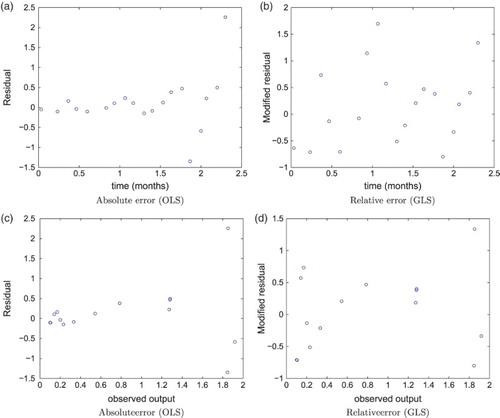
Next, we choose a relative error model and display the residual plots versus time and model output, respectively, for model A using $\gamma =0.85$ in Equation (6(6) ${\mathbf{\text{Y}}}_j=\mathbf{\text{f}}(t_j,\theta {\theta }_0)+{\mathbf{\text{f}}}^{\gamma }(t_j,\theta {\theta }_0)\circ {\mathcal{E}}_j,j=1,\dots ,n,$(6) ) (see Figure 2(b) and 2(d)). We choose γ by searching for the value that consistently produced i.i.d. residual plots given a range of parameter estimates. In our computations, $\gamma =0.85$ produces these results for both models (A and B). Although we only present here the residual plots for model A, the plots for model B exhibit very similar traits (see [7]). The reader may compare Figure 2(a) and 2(c) with Figure 2(b) and 2(d), respectively, to visualize the clear difference between the absolute and relative error statistical models. From these results, we assume a statistical model (6(6) ${\mathbf{\text{Y}}}_j=\mathbf{\text{f}}(t_j,\theta {\theta }_0)+{\mathbf{\text{f}}}^{\gamma }(t_j,\theta {\theta }_0)\circ {\mathcal{E}}_j,j=1,\dots ,n,$(6) ) with $\gamma =0.85$ for all subsequent analysis. When implementing this method, we choose the terminating tolerance in the GLS algorithm in the following manner: $\mathtt{s}\mathtt{t}\mathtt{o}\mathtt{p}\mathtt{i}\mathtt{f}max\mathtt{|}{\stackrel{\mathtt{ˆ}}{\theta \theta }}^{\mathtt{(}\mathtt{k}\mathtt{+}\mathtt{1}\mathtt{)}}\mathtt{-}{\stackrel{\mathtt{ˆ}}{\theta \theta }}^{\mathtt{\left(}\mathtt{k}\mathtt{\right)}}\mathtt{|}\mathtt{<}{\mathtt{10}}^{\mathtt{-}\mathtt{2}}\mathtt{,}$ where $max|\cdot |$ is the max-norm for vectors.

3.2. Mathematical model and parameter estimation

In order to estimate the true parameter vector $\theta {\theta }_0=[\eta ,{\lambda }_1,{\lambda }_2,{\lambda }_3{]}^T$, we find the parameter values which minimize the GLS cost functional (8(8) ${\tilde{J}}_n\left(\mathbf{\text{Y}}\right)=\frac{1}{n}\sum _{j=1}^n{\omega }_j[Y_j-f(t_j,\theta \theta ){]}^2$(8) ). Because of the stiff nature of the linear spline approximations, we utilize MATLAB's ODE solver ode15s. We consider both unconstrained and constrained optimization techniques for parameter estimation. In the case of unconstrained optimization, $\mathcal{Q}={\mathbb{R}}^p$, whereas for constrained optimization, $\mathcal{Q}$ is some strategic subset of ${\mathbb{R}}^p$, given the nature of the parameters. It is reasonable to presume that ${\lambda }_i<0$ for i=1,2,3, given the assumption that pesticide applications slow population growth. While non-negative values for ${\lambda }_i$ are not impossible (as in the case of hormesis [15]), they are generally unexpected. Therefore, to carry out constrained optimization, we let $\mathcal{Q}=\{\mathbb{R}\times [-\mathrm{\infty },ϵ{]}^3\}$. We use an upper bound of ε (some small positive value) rather than 0, to comply with an assumption of the model comparison test [1] and to permit mild hormetic effects. In practice, it is reasonable to further constrain $\mathcal{Q}=\{\mathbb{R}\times [-K,ϵ{]}^3\}$, where K is some positive finite number. Based on the estimates we found with a variety of initial guesses, we let K=20 in our constrained optimization search. In order to determine the best method, we also estimate parameters and calculate confidence intervals for each parameter using bootstrapping, which allows ones to look at the underlying distribution of each parameter (see [6] for details concerning both the theory and algorithm). For three out of the four parameters, the parameter estimate confidence intervals are significantly narrower when using constrained optimization in contrast to the confidence intervals found using bootstrapping with unconstrained optimization. Here, we estimate parameters and perform the model comparison test using MATLAB's constrained optimizing function, fmincon.

3.3. Model comparison results

We perform the model comparison test with r=3 degrees of freedom and p=4 parameters, using constrained optimization. We report the results using the relative error statistical model (6(6) ${\mathbf{\text{Y}}}_j=\mathbf{\text{f}}(t_j,\theta {\theta }_0)+{\mathbf{\text{f}}}^{\gamma }(t_j,\theta {\theta }_0)\circ {\mathcal{E}}_j,j=1,\dots ,n,$(6) ), and subsequently the incorrect statistical model (2(2) ${\mathbf{\text{Y}}}_j=\mathbf{\text{f}}(t_j,\theta {\theta }_0)+{\mathcal{E}}_j,j=1,\dots ,n,$(2) ) for the sake of comparison. In the computation of both optimization searches, we use ode15s to solve model A and ode45 to solve model B (due to the stiff nature of model A and non-stiff nature of model B). Consider $\mathcal{Q}$ as defined above (with optimization constraints) and define (14) ${\mathcal{Q}}_H=\{\theta \theta \in \mathcal{Q}|H\theta \theta =\mathbf{\text{c}}\},$(14) where $H=\left[\begin{array}{cccc}0& 1& 0& 0\\ 0& 0& 1& 0\\ 0& 0& 0& 1\end{array}\right],$ and $\mathbf{\text{c}}=\left[\begin{array}{c}0\\ 0\\ 0\end{array}\right]$. In other words, ${\mathcal{Q}}_H$ is the subset of $\mathcal{Q}$ such that ${\lambda }_i=0$ for i=1,2,3.

In comparison to highly controlled experimental data, ecological field data are more greatly affected by environmental factors, including weather changes and cross-field migration effects, none of which are incorporated into models A and B. Therefore one may argue that a larger significance value (e.g. $\alpha =0.1$) is a reasonable choice of significance. Using a ${\chi }^2\left(3\right)$ distribution table, we identify the corresponding threshold τ; given, $r=3,\alpha =0.1$, then $\tau =6.251$. The results are summarized in Table 2, where ‘Conf’ represents the confidence to reject the null hypothesis. As we have already noted above, one can equivalently carry out this test using $p-$values (see [4] for details). One can see that ${\hat{U}}_n=7.59>\tau$, therefore we can reject the null hypothesis with at least 90% confidence. In addition, we report the parameter estimates ${\widehat{\theta \theta }}^n$ and ${\widehat{\theta \theta }}_H^n$ in Table 3, as well as model fits to data for models A and B in Figure 3(a) and 3(b), respectively.

Figure 3. (a): Model A fit to data using relative error ($\gamma =0.85$) (b) model B (ignoring effects of pesticides) fit to data using relative error. Vertical dashed lines denote the time points at which pesticides were applied.

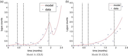
Table 2. Model comparison results using (best) relative error model and GLS.

$J_n$	$J_n^H$	${\hat{U}}_n$	Conf
0.30	0.42	7.59	94%

Table 3. Parameter estimates over admissible parameter spaces $\mathcal{Q}$ and ${\mathcal{Q}}_H$, using (best) relative error model and GLS.

Parameter space	η	${\lambda }_1$	${\lambda }_2$	${\lambda }_3$
$\mathcal{Q}$	3.7	−5.5	−10.4	−9.1
${\mathcal{Q}}_H$	1.8	0	0	0

We also present in Table 4 the results when using the incorrect statistical model. When assuming absolute error, we find ${\hat{U}}_n=1.46<\tau$, therefore we fail to reject the null hypothesis. As discussed below, this leads to a faulty conclusion regarding our primary goal in this study: the statistical significance of pesticide effects on L. hesperus populations, and reflecting this in the best choices of both statistical and mathematical models.

Table 4. Model comparison results, using (incorrect) absolute error model and OLS.

$J_n$	$J_n^H$	${\hat{U}}_n$	Conf
0.18	0.20	1.46	31%

4. Discussion

It is difficult to overemphasize the importance of carefully choosing the best statistical model. In ecology and many other disciplines, OLS (with an absolute error model) is a common method of parameter estimation, but GLS with a relative error statistical model is a better choice in many situations. A relative error model is not always best, and often an assumption of absolute error is sufficient. However, the statistical model will not only be critical in determining the resulting method to use in obtaining the parameter values, but will also affect every subsequent area of analysis, including model comparison results. Therefore, correct identification of the statistical model is imperative. In addition to the methods using residual plots seen above, there are other methods being explored to address this topic, including a technique that does not require prior parameter estimation [3]. In this case study, when incorrectly assuming an absolute error statistical model, the model comparison test results reported only 31% confidence to reject the null hypothesis, far below our desired threshold. Therefore, we fail to reject the null hypothesis. Based on these results, we could make one of the following incorrect conclusions: (a) the data does not support the estimation of time-dependent parameters or (b) model B best fits the data because pesticides did not have a significant effect on the population growth of L. hesperus.

However, it is clear that a relative error statistical model is a more accurate choice in this example, and the model comparison test results drive us toward the opposite conclusions: the data can support the estimation of time-dependent parameters, and a model incorporating the effects of pesticides does provide a statistically significantly better fit to the data than a simple exponential model. These conclusions are supported by the model fits presented in Figure 3. Although the exponential model does pick up the general increasing exponential nature of the data (see Figure 3(b)), the effects of pesticides are clearly non-trivial and should be represented in the mathematical model (see Figure 3(a)) and should not be overlooked, as in model B, in this case study.

In short, the statistical model defines the cost functional based on an assumed error structure, which defines the parameter estimates . All subsequent analyses, including math model selection, sensitivity analysis and other common studies, are heavily influenced by the assumptions of the statistical model describing the underlying error. Computationally, using GLS and a relative error model requires minimally more effort. Therefore, we stress that it is not only imperative, but easy to incorporate this important step into the modelling process.

In addition to statistical model selection, we also draw attention to the consideration of time-dependent parameters. Using flexible methods like linear splines to approximate unknown effects caused by manipulations to the system can provide better model fits to data. Use of time-dependent parameters can be considered for many ecological problems, especially those with mid-season changes, including, but not limited to, known migration patterns, addition or removal of some species, chemical changes, non-constant breeding, and distinct weather changes.

We may consider several different approaches toward expanding on the current results. First, it is recommended that we repeat the preceding analysis on other replicates, including those with 1,2, or 4 pesticide applications to produce a more robust study of the information content of our larger database. In other words, it is a beneficial exercise to determine if there is a correlation between parameter estimation accuracy/data information content (see also [8] for examples) and frequency of pesticide application. In addition, we would like to consider a 2-D compartmental model, as in previous research [9] and use the model comparison test to determine if the data can support time-dependent parameters for each age class. This could not only shed light on the class-specific effects of pesticides (on both nymphs and adults), but could also provide further insight into whether distinguishing between nymph and adult age classes during data collection is beneficial to understanding population dynamics, in the case of pesticide-treated fields. Moreover, we are exploring other methods of verifying correct statistical method in statistical model misspecification studies that do not rely on previous computation of the inverse problem. Lastly, we would like to use sensitivity analysis to determine sensitivity of the model output (population projection) to perturbations in parameter values. This could provide insight into the subtle effects of pesticide efficacy on L. hesperus population growth.

Acknowledgments

J.E. Banks thanks J.A. Rosenheim for hosting him during his sabbatical, and also extends thanks to the University of Washington, Tacoma for providing support for him during his sabbatical leave. The authors wish to acknowledge the efforts of two referees of an earlier version of this ms. whose comments resulted in improvements in the current version of this ms.

Disclosure statement

No potential conflict of interest was reported by the authors.

Additional information

Funding

This research was supported by the Air Force Office of Scientific Research under grant number [AFOSR FA9550-12-1-0188].

References

- H.T. Banks and B.G. Fitzpatrick, Statistical methods for model comparison in parameter estimation problems for distributed systems, J. Math. Biol. 28 (1990), pp. 501–527. doi: 10.1007/BF00164161
- H.T. Banks and H.T. Tran, Mathematical and Experimental Modeling of Physical and Biological Processes, CRC Press, New York, 2009.
- H.T. Banks, J. Catenacci, and S. Hu, Use of difference-based methods to explore statistical and mathematical model discrepancy in inverse problems, CRSC-TR15-05, Center for Research in Scientific Computation, N.C. State University, Raleigh, NC; Revised, Sept; J. Inverse Ill-Posed Problems, 2015, submitted.
- H.T. Banks, S. Hu, and W.C. Thompson, Modeling and Inverse Problems in the Presence of Uncertainty, CRC Press, New York, 2014.
- H.T. Banks, Z.R. Kenz, and W.C. Thompson, An extension of RSS-based model comparison tests for weighted least squares, Intl. J. Pure Appl. Math. 79 (2012), pp. 155–183.
- J.E. Banks, H.T. Banks, K. Rinnovatore, and C.M. Jackson, Optimal sampling frequency and timing of threatened tropical bird populations: A modeling approach, Ecol. Model. 303 (2014), pp. 70–77. doi: 10.1016/j.ecolmodel.2015.02.005
- H.T. Banks, J.E. Banks, J.A. Rosenheim, and K.A. Tillman, Modelling populations of Lygus hesperus on cotton fields in the San Joaquin Valley of California: The importance of statistical and mathematical model choice, CRSC-TR15-04, N.C. State University, Raleigh, NC, 2015.
- H.T. Banks, M. Doumic, C. Kruse, S. Prigent, and H. Rezaei, Information content in data sets for a nucleated-polymerization model, CRSC-TR14-15, N.C. State University, Raleigh, NC, November; J. Biological Dynamics (2015), 2014. doi:10.1080/17513758.2015.1050465.
- H.T. Banks, J.E. Banks, K. Link, J.A. Rosenheim, C. Ross, and K.A. Tillman, Model comparison tests to determine data information content CRSC-TR14-13, Appl. Math. Lett. 43 (2015), pp. 10–18. doi: 10.1016/j.aml.2014.11.002
- P.E. Blom, S.J. Fleischer, and Z. Smilowitz, Spatial and temporal dynamics of Colorado potato beetle (Coleoptera: Chrysomelidae) in fields with perimeter and spatially targeted insecticides, Environ. Entomol. 31 (2002), pp. 149–159. doi: 10.1603/0046-225X-31.1.149
- M. Brabec, A. Honěk, S. Pekár, and Z. Martinková, Population dynamics of aphids on cereals: Digging in the time-series data to reveal population regulation caused by temperature, PLoS One 9(9) (2014), p. e106228. doi: 10.1371/journal.pone.0106228
- J.D. Brawn, S.K. Robinson, and F.R. Thompson III, The role of disturbance in the ecology and conservation of birds, Annu. Rev. Ecol. Syst. 32 (2001), pp. 251–276. doi: 10.1146/annurev.ecolsys.32.081501.114031
- K. Burnham and D. Anderson, Model Selection and Multimodal Inference, 2nd ed., Springer, New York, 2002.
- R.J. Carroll and D. Ruppert, Transformation and Weighting in Regression, Chapman & Hall, New York, 1988.
- G.C. Cutler, Insects, insecticides and hormesis: Evidence and considerations for study, Dose-Response 11(2) (2013), pp. 154–177, PMC, Web, 13 May 2015. doi: 10.2203/dose-response.12-008.Cutler
- M. Davidian and D.M. Giltinan, Nonlinear Models for Repeated Measurement Data, Chapman and Hall, London, 2000.
- N. Desneux, A. Decourtye, and J.M. Delpuech, The sublethal effects of pesticides on beneficial arthropods, Annu. Rev. Entomol. 52 (2007), pp. 81–106. doi: 10.1146/annurev.ento.52.110405.091440
- I. Dinov, Chi-square (χ) table, Statistics Online Computational Resource, n.d. Web, 30 April 2015. Available at http://www.socr.ucla.edu/Applets.dir/ChiSquareTable.html.
- C.S. Elton, The Ecology of Invasions by Plants and Animals, Methuen, London, 1958, p. 18.
- V.E. Forbes and P. Calow, Is the per capita rate of increase a good measure of population-level effects in ecotoxicology? Environ. Toxicol. Chem. 18 (1999), pp. 1544–1556. doi: 10.1002/etc.5620180729
- V.E. Forbes, P. Calow, and R.M. Sibly, The extrapolation problem and how population modeling can help, Environ. Toxicol. Chem. 27 (2008), pp. 1987–1994. doi: 10.1897/08-029.1
- V.E. Forbes, P. Calow, V. Grimm, T. Hayashi, T. Jager, A. Palmpvist, R. Pastorok, D. Salvito, R. Sibly, J. Spromberg, J. Stark, and R.A. Stillman, Integrating population modeling into ecological risk assessment, Integr. Environ. Assess. Manag. 6 (2010), pp. 191–193. doi: 10.1002/ieam.25
- T.R. Grasswitz, Field evaluation of organically acceptable foliar insectides for control of green peach aphid, Arthropod Manag. Tests 39(1) (2014), p. B7. doi: 10.4182/amt.2014.B7
- M.P. Hassell, J.H. Lawton, and R.M. May, Patterns of dynamical behaviour in single-species populations, J. Anim. Ecol. (1976), pp. 471–486. doi: 10.2307/3886
- R. Hilborn, The Ecological Detective: Confronting Models with Data, Vol. 28, Princeton University Press, Princeton, NJ, 1997.
- S. Macfadyen, J.E. Banks, J.D. Stark, and A.P. Davies, Using semi-field studies to examine the effects of pesticides on mobile terrestrial invertebrates, Ann. Rev. Entomol. 59 (2014), pp. 383–404. doi: 10.1146/annurev-ento-011613-162109
- B.L. McManus and B.W. Fuller, Soybean aphid management using foliar applied insecticides in South Dakota, Arthropod Manag. Tests 38(1) (2013), p. F65.
- H. Motulsky and A. Christopoulos, Fitting Models to Biological Data Using Linear and Nonlinear Regression: A Practical Guide to Curve Fitting, Oxford University Press, New York, NY, 2004.
- S.T.A. Pickett and P.S. White, Natural disturbance and patch dynamics: An introduction, in The Ecology of Natural Disturbance and Patch Dynamics, S.T.A. Pickett and P.S. White, eds., Academic Press, Orlando, 1985, pp. 3–13.
- G.L. Reed, A.S. Jensen, J. Riebe, G. Head, and J.J. Duan, Transgenic Bt potato and conventional insecticides for Colorado potato beetle management: Comparative efficacy and non-target impacts, Entomologia Experimentalis et Applicata 100(1) (2001), pp. 89–100. doi: 10.1046/j.1570-7458.2001.00851.x
- J.A. Rosenheim, K. Steinmann, G.A. Langelloto, and A.G. Zink, Estimating the impact of Lygus hesperus on cotton: The insect, plant and human observer as sources of variability, Environ. Entomol. 35 (2006), pp. 1141–1153. doi: 10.1603/0046-225X(2006)35[1141:ETIOLH]2.0.CO;2
- G.A.F. Seber and C.J. Wild, Nonlinear Regression, J. Wiley & Sons, Hoboken, NJ, 2003.
- S.F. Smith and V.A. Krischik, Effects of systemic imidacloprid on Coleomegilla maculata (Coleoptera: Coccinellidae), Environ. Entomol. 28 (1999), pp. 1189–1195. doi: 10.1093/ee/28.6.1189
- J.D. Stark and J.E. Banks, Population-level effects of pesticides and other toxicants on arthropods, Annu. Rev. Entomol. 48 (2003), pp. 505–519. doi: 10.1146/annurev.ento.48.091801.112621
- J.D. Stark, J.E. Banks, and R. Vargas, How risky is risk assessment: The role that life history strategies play in susceptibility of species to stress, Proc. Natl. Acad. Sci. 101 (2004), pp. 732–736. doi: 10.1073/pnas.0304903101
- J.D. Stark, R. Vargas, and J.E. Banks, Incorporating ecologically relevant measures of pesticide effect for estimating the compatibility of pesticides and biocontrol agents, J. Econ. Entomol. 100(4) (2007), pp. 1027–1032. doi: 10.1093/jee/100.4.1027
- J.D. Stark, R.I. Vargas, and J.E. Banks, Incorporating variability in point estimates in risk assessment: Bridging the gap between LC50 and population endpoints, Environ. Toxicol. Chem. 34(7) (2015), pp. 1683–1688. doi: 10.1002/etc.2978
- M.R.E. Symonds and A. Moussalli, A brief guide to model selection, mulitimodal interference and model averaging in behavioural ecology using Akaike's information criterion, Behav. Ecol. Sociobiol. 65(1) (2011), pp. 13–21. doi: 10.1007/s00265-010-1037-6
- K.M. Theiling and B.A. Croft, Pesticide side effects on arthropod natural enemies: A database summary, Agric. Ecosyst. Environ. 21 (1998), pp. 191–218. doi: 10.1016/0167-8809(88)90088-6
- E.W. Weisstein, Chi-squared distribution, From MathWorld–A Wolfram Web Resource. Available at http://mathworld.wolfram.com/Chi-SquaredDistribution.html.
- K. Zhou, J. Huang, X. Deng, W. van der Werf, W. Zhang, Y. Lu, K. Wu, and F. Wu, Effects of land use and insecticides on natural enemies of aphids in cotton: First evidence from smallholder agriculture in the North China Plain, Agric. Ecosyst. Environ. 183 (2014), pp. 176–184. doi: 10.1016/j.agee.2013.11.008