Analysis of HIV models with two time delays

ABSTRACT

Time delays can affect the dynamics of HIV infection predicted by mathematical models. In this paper, we studied two mathematical models each with two time delays. In the first model with HIV latency, one delay is the time between viral entry into a cell and the establishment of HIV latency, and the other delay is the time between cell infection and viral production. We defined the basic reproductive number and showed the local and global stability of the steady states. Numerical simulations were performed to evaluate the influence of time delays on the dynamics. In the second model with HIV immune response, one delay is the time between cell infection and viral production, and the other delay is the time needed for the adaptive immune response to emerge to control viral replication. With two positive delays, we obtained the stability crossing curves for the model, which were shown to be a series of open-ended curves.

KEYWORDS:

• HIV infection
• latency
• immune response
• characteristic quasipolynomial
• stability
• stability crossing curve

AMS SUBJECT CLASSIFICATION:

• 92B05
• 92D25
• 92C37
• 34D23

1. Introduction

Human immunodeficiency virus type 1 (HIV-1) infects CD4+ T cells, a substantial component of the immune system, and the infection goes through three distinct stages (see review in [31]): primary infection, asymptomatic stage, and acquired immunodeficiency syndrome (AIDS). The primary infection stage lasts a few weeks during which the viral load in blood increases rapidly to the peak level, followed by decline to a steady state. CD4+ T cells decrease initially because of the infection and then undergo a minor increase as the primary infection ends. A high level of viral infection stimulates the development of adaptive immune responses, including CD8+ T cells, which can kill infected cells [55]. The asymptomatic infection stage can take several years, in which there is usually a very slow increase in the viral load and a slow decline in CD4+ T cells. As CD4+ T cells decline to a low level, for example, 200 cells per microlitre, the AIDS stage begins [10]. Infected individuals have a rapid increase in plasma viral load and are also accompanied with various opportunistic infections because of the collapse of the immune system. Current treatment consisting of several antiretroviral drugs can suppress viral load to below the detection limit of standard assays but cannot eradicate the virus. An important reason is that HIV can persist as provirus in resting memory CD4+ T cells [7, 13, 56]. These latently infected CD4+ T cells live relatively long, are not affected by antiretroviral therapy, but can be activated by their relevant antigens to produce new virions [4].

Mathematical models have been developed to study the dynamics of virions and CD4+ T cells during infection, the influence of antiretroviral therapy, the emergence of drug resistance, immune responses, and low viral load persistence in patients receiving prolonged antiretroviral therapy (see reviews in [34–36, 43]). Many models assumed that cells produce virus immediately after they are infected. However, the life cycle of the virus contains a number of intracellular processes; for example, viral entry into a target cell, reverse transcription from HIV RNA to DNA, integration of viral DNA into the host cell's DNA, transcription and translation, assembly and virus budding from the infected cell [34]. A time delay representing the time between cell infection and viral production has been incorporated into models to study its influence on virus dynamics. Assuming that the target CD4+ T cell level is constant and that the treatment is 100% effective in the delay model, Herz et al. obtained the analytic expression of the viral load decline under treatment and used it to analyse the viral load decline data in patients [18]. Nelson et al. extended the analysis and showed that the time delay can affect the estimate of the death rate of infected cells when treatment is not 100% effective [29]. A distributed continuous time delay was used to account for the different time between cell infection and viral production [15, 27, 28]. More models including the intracellular delay can be found in refs. [3, 11, 12, 20–23, 25, 49, 51–54, 57] and references cited therein.

The adaptive immune responses need time to emerge to control viral replication [55]. Ciupe et al. [8] included a time delay representing the time needed to activate the CD8+ T cell response in a model. Pawelek et al. [33] incorporated two delays, one the time needed for infected cells to produce virus and the other the time needed for CD8+ T cells to emerge to kill infected cells. The model was fit to the viral load data from patients during primary infection. Some special cases of the model with two delays have been mathematically analysed [33]. However, the stability switching curves for the infected steady state when both delays are positive have not been investigated.

In this paper, we will study two HIV models each with two time delays. In the first model, we incorporate two time delays into an HIV latent infection model which was introduced to evaluate the contribution of latently infected cell activation to HIV production [38]. One delay is the time between viral entry into a cell and the establishment of HIV latency (i.e. the viral DNA has been integrated into the host cell's DNA), and the other delay is the time between initial cell infection and viral production. We will investigate the local and global stability of the steady states. Numerical simulations will be performed to evaluate the influence of time delays on the dynamics. The second model of HIV immune response with two delays is the same as that in ref. [33]. Some special cases of the model have been studied before [33]. Here we will use the method developed by Gu et al. [16] to determine the stability crossing curves for the infected steady state of the model when both delays are positive.

2. An HIV latent infection model with two delays

In this section, we study an HIV latent infection model with two time delays. The model without delays was introduced to analyse the biphasic viral load decline observed in patients receiving combination therapy of two reverse transcriptase inhibitors and one protease inhibitor [38]. It was mathematically analysed in ref. [32]. The model assumes that once infected, the cell immediately becomes either a productively infected cell that can produce virus, or becomes a latently infected cell that can be activated to produce virus. However, it takes time for the latent infection to be established and also for productively infected cells to produce virus. We introduce two time delays into the model. One is the time between viral entry and latent infection (i.e. the integration of viral DNA into cell's DNA has finished) and the other is the time between viral entry and viral production. The first delay is denoted by ${\tau }_1$ and the second delay is denoted by ${\tau }_2$. Obviously, we have ${\tau }_1<{\tau }_2$ from the viral life cycle. The model can be described by the following system of delayed differential equations. (1) $\begin{array}{rl}\frac{\mathrm{d}T}{\mathrm{d}t}& =s-d_{T}T-\beta VT,\\ \frac{\mathrm{d}L}{\mathrm{d}t}& =f\beta V(t-{\tau }_1)T(t-{\tau }_1){\mathrm{e}}^{-{\delta }_1{\tau }_1}-{\delta }_{L}L-\alpha L,\\ \frac{\mathrm{d}I}{\mathrm{d}t}& =(1-f)\beta V(t-{\tau }_2)T(t-{\tau }_2){\mathrm{e}}^{-{\delta }_1{\tau }_2}-\delta I+\alpha L,\\ \frac{\mathrm{d}V}{\mathrm{d}t}& =N\delta I-cV.\end{array}$(1)

In the model, $T\left(t\right)$ is the concentration of uninfected CD4+ T cells at time t, $L\left(t\right)$ denotes the concentration of latently infected T cells at time t, $I\left(t\right)$ is the concentration of productively infected cells, and $V\left(t\right)$ represents the concentration of virions in plasma at t. The parameter s is the generate rate of uninfected CD4+ T cells, $d_T$ is the per capita death rate of uninfected cells, and β is the infection rate of target cell by virus. A small fraction (f) of infected cells are assumed to result in latency and the remaining become productively infected cells. Latently infected cells die at a rate constant ${\delta }_L$ per cell and productively infected cells die at a rate constant δ per cell. N is the viral burst size, which is the total number of virions released by one infected cell in its lifespan, and c is the viral clearance rate. Latently infected cells can be activated by their relevant antigens to become productively infected cells at a rate constant α. The parameter ${\delta }_1$ represents the death rate of infected cells that have not started to produce virus. Thus, ${\mathrm{e}}^{-{\delta }_1{\tau }_1}$ and ${\mathrm{e}}^{-{\delta }_1{\tau }_2}$ represent the probability of an infected cells surviving the time ${\tau }_1$ and ${\tau }_2$, respectively, following viral entry. Parameters and values used in simulations are summarized in Table 1.

Table 1. Parameters and values used in the models and simulations.

Parameter	Description	Value and unit	References
s	Generation rate of uninfected cells	${10}^4$ cell ml^−1 day^−1	See text
$d_{\mathrm{T}}$	Death rate of uninfected cells	0.01 day^−1	[37]
β	Infection rate	$2.4\times {10}^{-8}$ ml virion^−1 day^−1	[44]
f	Fraction of latency	0.001	[41]
δ	Death rate of infected cells	1 day^−1	[26]
α	Activation rate of latently infected cells	0.01 day^−1	[43]
${\delta }_{\mathrm{L}}$	Death rate of latently infected cells	$4\times {10}^{-3}$ day^−1	See text
${\delta }_1$	Death rate of infected cells that have not started to produce virus	0.05 day^−1	See text
N	Viral burst size	2000 virion cell^−1	[44]
c	Viral clearance rate	23 day^−1	[39]
$d_{\mathrm{E}}$	Death rate of effector cells	0.45 day^−1	[33]
p	Generation rate of effector cells	0.05 day^−1	[33]
$d_x$	Killing rate by effector cells	$3.7\times {10}^{-4}$ ml cell day^−1	[33]

We derive the basic reproductive number using the next-generation method. From the infection and viral production term in the model, we define matrices $\mathbb{F}$ and $\mathbb{V}$ as follows $\mathbb{F}=\left(\begin{array}{ccc}0& 0& f\beta T_0{\mathrm{e}}^{-{\delta }_1{\tau }_1}\\ 0& 0& (1-f)\beta T_0{\mathrm{e}}^{-{\delta }_1{\tau }_2}\\ 0& 0& 0\end{array}\right),\mathbb{V}=\left(\begin{array}{ccc}\alpha +{\delta }_L& 0& 0\\ -\alpha & \delta & 0\\ 0& -N\delta & c\end{array}\right),$ where $T_0=s/d_T$ is the steady-state level of target cells before infection. The basic reproductive number, $R_0$, can be derived as the spectral radius of the next generation operator $\mathbb{F}{\mathbb{V}}^{-1}$. Straightforward calculation yields $\mathbb{F}{\mathbb{V}}^{-1}=\left(\begin{array}{ccc}f\beta T_0{\mathrm{e}}^{-{\delta }_1{\tau }_1}\frac{N\alpha }{c(\alpha +{\delta }_L)}& f\beta T_0{\mathrm{e}}^{-{\delta }_1{\tau }_1}\frac{N}{c}& f\beta T_0{\mathrm{e}}^{-{\delta }_1{\tau }_1}\frac{1}{c}\\ (1-f)\beta T_0{\mathrm{e}}^{-{\delta }_1{\tau }_2}\frac{N\alpha }{c(\alpha +{\delta }_L)}& (1-f)\beta T_0{\mathrm{e}}^{-{\delta }_1{\tau }_2}\frac{N}{c}& (1-f)\beta T_0{\mathrm{e}}^{-{\delta }_1{\tau }_2}\frac{1}{c}\\ 0& 0& 0\end{array}\right).$

Thus, $R_0$ is given by (2) $R_0=\frac{s\beta N}{c{d}_T}\cdot \left[(1-f){\mathrm{e}}^{-{\delta }_1{\tau }_2}+\frac{\alpha }{{\delta }_L+\alpha }f{\mathrm{e}}^{-{\delta }_1{\tau }_1}\right].$(2) Notice that $s\beta N/c{d}_T$ is the basic reproductive number of the basic model (i.e. model (1(1) $\begin{array}{rl}\frac{\mathrm{d}T}{\mathrm{d}t}& =s-d_{T}T-\beta VT,\\ \frac{\mathrm{d}L}{\mathrm{d}t}& =f\beta V(t-{\tau }_1)T(t-{\tau }_1){\mathrm{e}}^{-{\delta }_1{\tau }_1}-{\delta }_{L}L-\alpha L,\\ \frac{\mathrm{d}I}{\mathrm{d}t}& =(1-f)\beta V(t-{\tau }_2)T(t-{\tau }_2){\mathrm{e}}^{-{\delta }_1{\tau }_2}-\delta I+\alpha L,\\ \frac{\mathrm{d}V}{\mathrm{d}t}& =N\delta I-cV.\end{array}$(1) ) without latently infected cells and without time delays, see ref. [44]), $(1-f){\mathrm{e}}^{-{\delta }_1{\tau }_2}$ is the contribution to the basic reproductive number from productively infected cells, and $\left(\alpha /({\delta }_L+\alpha )\right)f{\mathrm{e}}^{-{\delta }_1{\tau }_1}$ represents the contribution from activation of latently infected cells. Therefore, $R_0$ is the basic reproductive number of model (1(1) $\begin{array}{rl}\frac{\mathrm{d}T}{\mathrm{d}t}& =s-d_{T}T-\beta VT,\\ \frac{\mathrm{d}L}{\mathrm{d}t}& =f\beta V(t-{\tau }_1)T(t-{\tau }_1){\mathrm{e}}^{-{\delta }_1{\tau }_1}-{\delta }_{L}L-\alpha L,\\ \frac{\mathrm{d}I}{\mathrm{d}t}& =(1-f)\beta V(t-{\tau }_2)T(t-{\tau }_2){\mathrm{e}}^{-{\delta }_1{\tau }_2}-\delta I+\alpha L,\\ \frac{\mathrm{d}V}{\mathrm{d}t}& =N\delta I-cV.\end{array}$(1) ).

The model has two equilibrium points. One is the infection-free equilibrium $E_0=(T_0,0,0,0)$ and the other is the infected equilibrium $E^{\ast }=(T^{\ast },L^{\ast },I^{\ast },V^{\ast })$, where (3) $\begin{array}{rl}{T}^{\ast }& =\frac{s}{d_T{R}_0},\\ L^{\ast }& =\frac{sf{\mathrm{e}}^{-{\delta }_1{\tau }_1}}{R_0({\delta }_L+\alpha )}(R_0-1),\\ I^{\ast }& =\frac{d_{T}c}{\beta N\delta }(R_0-1),\\ V^{\ast }& =\frac{d_T}{\beta }(R_0-1).\end{array}$(3) It is clear that the infected steady state exists if and only if $R_0>1$.

3. Stability analysis

3.1. Local stability

In this section, we study the local stability of the infection-free equilibrium and the infected equilibrium points. The following result suggests that the basic reproductive number provides a threshold value determining if the infection is predicted to die out or persist.

Theorem 3.1.

The infection-free equilibrium $E_0$ of model (1(1) $\begin{array}{rl}\frac{\mathrm{d}T}{\mathrm{d}t}& =s-d_{T}T-\beta VT,\\ \frac{\mathrm{d}L}{\mathrm{d}t}& =f\beta V(t-{\tau }_1)T(t-{\tau }_1){\mathrm{e}}^{-{\delta }_1{\tau }_1}-{\delta }_{L}L-\alpha L,\\ \frac{\mathrm{d}I}{\mathrm{d}t}& =(1-f)\beta V(t-{\tau }_2)T(t-{\tau }_2){\mathrm{e}}^{-{\delta }_1{\tau }_2}-\delta I+\alpha L,\\ \frac{\mathrm{d}V}{\mathrm{d}t}& =N\delta I-cV.\end{array}$(1) ) is locally asymptotically stable when $R_0<1$ and unstable when $R_0>1$.

Proof.

We linearize the system (1(1) $\begin{array}{rl}\frac{\mathrm{d}T}{\mathrm{d}t}& =s-d_{T}T-\beta VT,\\ \frac{\mathrm{d}L}{\mathrm{d}t}& =f\beta V(t-{\tau }_1)T(t-{\tau }_1){\mathrm{e}}^{-{\delta }_1{\tau }_1}-{\delta }_{L}L-\alpha L,\\ \frac{\mathrm{d}I}{\mathrm{d}t}& =(1-f)\beta V(t-{\tau }_2)T(t-{\tau }_2){\mathrm{e}}^{-{\delta }_1{\tau }_2}-\delta I+\alpha L,\\ \frac{\mathrm{d}V}{\mathrm{d}t}& =N\delta I-cV.\end{array}$(1) ), obtain the Jacobian matrix J at the infection-free steady state $E_0$, and calculate the matrix $\lambda I-J\left(E_0\right)$ as follows, where λ is the eigenvalue and I is the identity matrix with the same dimension as $J\left(E_0\right)$. $\lambda I-J\left(E_0\right)=\left(\begin{array}{cccc}\lambda +d_T& 0& 0& \beta s/d_T\\ 0& \lambda +{\delta }_L+\alpha & 0& -\frac{\beta fs}{d_T}{\mathrm{e}}^{-{\delta }_1{\tau }_1}{\mathrm{e}}^{-{\tau }_1\lambda }\\ 0& -\alpha & \lambda +\delta & -\frac{\beta (1-f)s}{d_T}{\mathrm{e}}^{-{\delta }_1{\tau }_2}{\mathrm{e}}^{-{\tau }_2\lambda }\\ 0& 0& -N\delta & \lambda +c\end{array}\right).$ Thus, the characteristic equation at the equilibrium $E_0$ is given by (4) $\begin{array}{rl}0& =|\lambda I-J\left(E_0\right)|\\ & =(\lambda +d_T)\left[(\lambda +{\delta }_L+\alpha )(\lambda +c)(\lambda +\delta )-\frac{\alpha N\delta \beta fs}{d_T}{\mathrm{e}}^{-{\delta }_1{\tau }_1}{\mathrm{e}}^{-{\tau }_1\lambda }\right.\\ & -\left.(\lambda +{\delta }_L+\alpha )\frac{N\beta (1-f)s\delta }{d_T}{\mathrm{e}}^{-{\delta }_1{\tau }_2}{\mathrm{e}}^{-{\tau }_2\lambda }\right].\end{array}$(4) When ${\tau }_1={\tau }_2=0$, the infection-free equilibrium $E_0$ of Equation (1(1) $\begin{array}{rl}\frac{\mathrm{d}T}{\mathrm{d}t}& =s-d_{T}T-\beta VT,\\ \frac{\mathrm{d}L}{\mathrm{d}t}& =f\beta V(t-{\tau }_1)T(t-{\tau }_1){\mathrm{e}}^{-{\delta }_1{\tau }_1}-{\delta }_{L}L-\alpha L,\\ \frac{\mathrm{d}I}{\mathrm{d}t}& =(1-f)\beta V(t-{\tau }_2)T(t-{\tau }_2){\mathrm{e}}^{-{\delta }_1{\tau }_2}-\delta I+\alpha L,\\ \frac{\mathrm{d}V}{\mathrm{d}t}& =N\delta I-cV.\end{array}$(1) ) was shown to be locally asymptotically stable when $R_0<1$ and unstable when $R_0>1$ according to the Routh–Hurwitz stability criterion [32]. Next, we show that the conclusion holds for any ${\tau }_1>0$ and ${\tau }_2>0$.

It is clear that Equation (4(4) $\begin{array}{rl}0& =|\lambda I-J\left(E_0\right)|\\ & =(\lambda +d_T)\left[(\lambda +{\delta }_L+\alpha )(\lambda +c)(\lambda +\delta )-\frac{\alpha N\delta \beta fs}{d_T}{\mathrm{e}}^{-{\delta }_1{\tau }_1}{\mathrm{e}}^{-{\tau }_1\lambda }\right.\\ & -\left.(\lambda +{\delta }_L+\alpha )\frac{N\beta (1-f)s\delta }{d_T}{\mathrm{e}}^{-{\delta }_1{\tau }_2}{\mathrm{e}}^{-{\tau }_2\lambda }\right].\end{array}$(4) ) has a negative root $\lambda =-d_T$. All the other roots are determined by the following equation (5) $(\lambda +{\delta }_L+\alpha )\left[(\lambda +c)(\lambda +\delta )-\frac{N\beta (1-f)s\delta }{d_T}{\mathrm{e}}^{-{\delta }_1{\tau }_2}{\mathrm{e}}^{-{\tau }_2\lambda }\right]=\frac{\alpha N\delta \beta fs}{d_T}{\mathrm{e}}^{-{\delta }_1{\tau }_1}{\mathrm{e}}^{-{\tau }_1\lambda }.$(5)

For simplicity, we introduce a new notation (6) $g=\frac{(1-f)({\delta }_L+\alpha ){\mathrm{e}}^{-{\delta }_1{\tau }_2}}{(1-f)({\delta }_L+\alpha ){\mathrm{e}}^{-{\delta }_1{\tau }_2}+\alpha f{\mathrm{e}}^{-{\delta }_1{\tau }_1}}.$(6)

Obviously, we have 0<g<1. Using the notation g and the basic reproductive number $R_0$, the characteristic equation  (5(5) $(\lambda +{\delta }_L+\alpha )\left[(\lambda +c)(\lambda +\delta )-\frac{N\beta (1-f)s\delta }{d_T}{\mathrm{e}}^{-{\delta }_1{\tau }_2}{\mathrm{e}}^{-{\tau }_2\lambda }\right]=\frac{\alpha N\delta \beta fs}{d_T}{\mathrm{e}}^{-{\delta }_1{\tau }_1}{\mathrm{e}}^{-{\tau }_1\lambda }.$(5) ) can be simplified as (7) $(\lambda +{\delta }_L+\alpha )\left(\right(\lambda +c\left)\right(\lambda +\delta )-c\delta g{\mathrm{e}}^{-{\tau }_2\lambda }{R}_0)=c\delta (1-g)({\delta }_L+\alpha ){\mathrm{e}}^{-{\tau }_1\lambda }{R}_0.$(7)

Suppose that the real part of the eigenvalue λ is non-negative. Taking the modulus of the left-hand side of Equation (7(7) $(\lambda +{\delta }_L+\alpha )\left(\right(\lambda +c\left)\right(\lambda +\delta )-c\delta g{\mathrm{e}}^{-{\tau }_2\lambda }{R}_0)=c\delta (1-g)({\delta }_L+\alpha ){\mathrm{e}}^{-{\tau }_1\lambda }{R}_0.$(7) ) and also using Cauchy–Schwartz inequality, we obtain (8) $\begin{array}{rl}|\lambda +{\delta }_L+\alpha ||(\lambda +c)(\lambda +\delta )-c\delta g{\mathrm{e}}^{-{\tau }_2\lambda }{R}_0|& \ge ({\delta }_L+\alpha )||\lambda +c||\lambda +\delta |-|c\delta g{\mathrm{e}}^{-{\tau }_2\lambda }{R}_0||\\ & \ge ({\delta }_L+\alpha )||\lambda +c||\lambda +\delta |-c\delta g{R}_0|\\ & =({\delta }_L+\alpha )(|\lambda +c||\lambda +\delta |-c\delta g{R}_0)\\ & \ge c\delta ({\delta }_L+\alpha )(1-g).\end{array}$(8)

On the other hand, the modulus of the right-hand side of Equation (7(7) $(\lambda +{\delta }_L+\alpha )\left(\right(\lambda +c\left)\right(\lambda +\delta )-c\delta g{\mathrm{e}}^{-{\tau }_2\lambda }{R}_0)=c\delta (1-g)({\delta }_L+\alpha ){\mathrm{e}}^{-{\tau }_1\lambda }{R}_0.$(7) ) satisfies (9) $|c\delta (1-g)({\delta }_L+\alpha ){\mathrm{e}}^{-{\tau }_1\lambda }{R}_0|<c\delta ({\delta }_L+\alpha )(1-g).$(9) That leads to a contradiction. It follows that all the roots of the characteristic equation  (4(4) $\begin{array}{rl}0& =|\lambda I-J\left(E_0\right)|\\ & =(\lambda +d_T)\left[(\lambda +{\delta }_L+\alpha )(\lambda +c)(\lambda +\delta )-\frac{\alpha N\delta \beta fs}{d_T}{\mathrm{e}}^{-{\delta }_1{\tau }_1}{\mathrm{e}}^{-{\tau }_1\lambda }\right.\\ & -\left.(\lambda +{\delta }_L+\alpha )\frac{N\beta (1-f)s\delta }{d_T}{\mathrm{e}}^{-{\delta }_1{\tau }_2}{\mathrm{e}}^{-{\tau }_2\lambda }\right].\end{array}$(4) ) have negative real parts. Thus, the infection-free steady state is locally asymptotically stable when $R_0<1$.

Next, we turn to the case of $R_0>1$ with delays ${\tau }_1>0$ and ${\tau }_2>0$. The characteristic equation  (4(4) $\begin{array}{rl}0& =|\lambda I-J\left(E_0\right)|\\ & =(\lambda +d_T)\left[(\lambda +{\delta }_L+\alpha )(\lambda +c)(\lambda +\delta )-\frac{\alpha N\delta \beta fs}{d_T}{\mathrm{e}}^{-{\delta }_1{\tau }_1}{\mathrm{e}}^{-{\tau }_1\lambda }\right.\\ & -\left.(\lambda +{\delta }_L+\alpha )\frac{N\beta (1-f)s\delta }{d_T}{\mathrm{e}}^{-{\delta }_1{\tau }_2}{\mathrm{e}}^{-{\tau }_2\lambda }\right].\end{array}$(4) ) can be written as the following quasipolynomial (10) ${\lambda }^3+A_1{\lambda }^2+A_2\lambda +A_3=0,$(10) where $\begin{array}{rl}{A}_1& =c+\delta +{\delta }_L+\alpha ,\\ A_2& =c\delta +({\delta }_L+\alpha )(\delta +c)-\frac{N\beta (1-f)s\delta }{d_T}{\mathrm{e}}^{-{\delta }_1{\tau }_2}{\mathrm{e}}^{-{\tau }_2\lambda },\\ A_3& =c\delta ({\delta }_L+\alpha )-\frac{sN\beta \delta }{d_T}\left(\right(1-f\left)\right({\delta }_L+\alpha ){\mathrm{e}}^{-{\delta }_1{\tau }_2}{\mathrm{e}}^{-{\tau }_2\lambda }+\alpha f{\mathrm{e}}^{-{\delta }_1{\tau }_1}{\mathrm{e}}^{-{\tau }_1\lambda }).\end{array}$ When $R_0>1$, we define a function $p\left(\lambda \right)={\lambda }^3+A_1{\lambda }^2+A_2\lambda +A_3$. It can be seen that $p\left(\lambda \right)\to \mathrm{\infty }$ as $\lambda \to \mathrm{\infty }$ and $p\left(0\right)=A_3=c\delta ({\delta }_L+\alpha )(1-R_0)<0$. Thus, there is at least one positive real root. This shows that the inflection-free steady-state $E_0$ is unstable when $R_0>1$.

From the expressions in Equation (3(3) $\begin{array}{rl}{T}^{\ast }& =\frac{s}{d_T{R}_0},\\ L^{\ast }& =\frac{sf{\mathrm{e}}^{-{\delta }_1{\tau }_1}}{R_0({\delta }_L+\alpha )}(R_0-1),\\ I^{\ast }& =\frac{d_{T}c}{\beta N\delta }(R_0-1),\\ V^{\ast }& =\frac{d_T}{\beta }(R_0-1).\end{array}$(3) ), we know that the infected steady state exists if and only if $R_0>1$. The following result shows that the chronic infection is established when $R_0>1$.

Theorem 3.2.

The infected equilibrium $E^{\ast }$ of Equation (1(1) $\begin{array}{rl}\frac{\mathrm{d}T}{\mathrm{d}t}& =s-d_{T}T-\beta VT,\\ \frac{\mathrm{d}L}{\mathrm{d}t}& =f\beta V(t-{\tau }_1)T(t-{\tau }_1){\mathrm{e}}^{-{\delta }_1{\tau }_1}-{\delta }_{L}L-\alpha L,\\ \frac{\mathrm{d}I}{\mathrm{d}t}& =(1-f)\beta V(t-{\tau }_2)T(t-{\tau }_2){\mathrm{e}}^{-{\delta }_1{\tau }_2}-\delta I+\alpha L,\\ \frac{\mathrm{d}V}{\mathrm{d}t}& =N\delta I-cV.\end{array}$(1) ) is locally asymptotically stable when it exists $($i.e. when $R_0>1)$.

Proof.

Similar to the infection-free steady state, we obtain the Jacobian matrix at the infected steady-state $E^{\ast }$ and calculate the matrix $\lambda I-J\left(E^{\ast }\right)$, given by $\begin{array}{rl}& \lambda I-J\left(E^{\ast }\right)\\ & =\left(\begin{array}{cccc}\lambda +d_T+\beta V^{\ast }& 0& 0& \beta T^{\ast }\\ -f\beta V^{\ast }{\mathrm{e}}^{-{\delta }_1{\tau }_1}{\mathrm{e}}^{-{\tau }_1\lambda }& \lambda +{\delta }_L+\alpha & 0& -\beta f{T}^{\ast }{\mathrm{e}}^{-{\delta }_1{\tau }_1}{\mathrm{e}}^{-{\tau }_1\lambda }\\ -(1-f)\beta V^{\ast }{\mathrm{e}}^{-{\delta }_1{\tau }_2}{\mathrm{e}}^{-{\tau }_2\lambda }& -\alpha & \lambda +\delta & -\beta (1-f)T^{\ast }{\mathrm{e}}^{-{\delta }_1{\tau }_2}{\mathrm{e}}^{-{\tau }_2\lambda }\\ 0& 0& -N\delta & \lambda +c\end{array}\right),\end{array}$ where λ is the eigenvalue, $V^{\ast }$ and $T^{\ast }$ are given in Equation (3(3) $\begin{array}{rl}{T}^{\ast }& =\frac{s}{d_T{R}_0},\\ L^{\ast }& =\frac{sf{\mathrm{e}}^{-{\delta }_1{\tau }_1}}{R_0({\delta }_L+\alpha )}(R_0-1),\\ I^{\ast }& =\frac{d_{T}c}{\beta N\delta }(R_0-1),\\ V^{\ast }& =\frac{d_T}{\beta }(R_0-1).\end{array}$(3) ). Using the basic reproductive number $R_0$, the characteristic equation at the infected steady state $E^{\ast }$ is (11) $\begin{array}{rl}0& =|\lambda I-J\left(E^{\ast }\right)|\\ & =(\lambda +d_T{R}_0)(\lambda +\delta )(\lambda +{\delta }_L+\alpha )(\lambda +c)\\ & -\frac{N\beta s\delta }{d_T{R}_0}\left(\right(1-f\left)\right(\lambda +{\delta }_L+\alpha ){\mathrm{e}}^{-{\delta }_1{\tau }_2}{\mathrm{e}}^{-{\tau }_2\lambda }+\alpha f{\mathrm{e}}^{-{\delta }_1{\tau }_1}{\mathrm{e}}^{-{\tau }_1\lambda })(\lambda +d_T).\end{array}$(11)

When ${\tau }_1={\tau }_2=0$ the infected equilibrium $E^{\ast }$ of model (1(1) $\begin{array}{rl}\frac{\mathrm{d}T}{\mathrm{d}t}& =s-d_{T}T-\beta VT,\\ \frac{\mathrm{d}L}{\mathrm{d}t}& =f\beta V(t-{\tau }_1)T(t-{\tau }_1){\mathrm{e}}^{-{\delta }_1{\tau }_1}-{\delta }_{L}L-\alpha L,\\ \frac{\mathrm{d}I}{\mathrm{d}t}& =(1-f)\beta V(t-{\tau }_2)T(t-{\tau }_2){\mathrm{e}}^{-{\delta }_1{\tau }_2}-\delta I+\alpha L,\\ \frac{\mathrm{d}V}{\mathrm{d}t}& =N\delta I-cV.\end{array}$(1) ) was shown to be locally asymptotically stable when $R_0>1$ (see [32]). We consider the case of $R_0>1$ with ${\tau }_1>0$ and ${\tau }_2>0$. Suppose that the eigenvalue λ has a non-negative real part. The characteristic equation  (11(11) $\begin{array}{rl}0& =|\lambda I-J\left(E^{\ast }\right)|\\ & =(\lambda +d_T{R}_0)(\lambda +\delta )(\lambda +{\delta }_L+\alpha )(\lambda +c)\\ & -\frac{N\beta s\delta }{d_T{R}_0}\left(\right(1-f\left)\right(\lambda +{\delta }_L+\alpha ){\mathrm{e}}^{-{\delta }_1{\tau }_2}{\mathrm{e}}^{-{\tau }_2\lambda }+\alpha f{\mathrm{e}}^{-{\delta }_1{\tau }_1}{\mathrm{e}}^{-{\tau }_1\lambda })(\lambda +d_T).\end{array}$(11) ) can be written as (12) $\begin{array}{rl}& (\lambda +{\delta }_L+\alpha )\left[\frac{\lambda +d_T{R}_0}{\lambda +d_T}(\lambda +\delta )(\lambda +c)-\frac{N\beta s\delta }{d_T{R}_0}(1-f){\mathrm{e}}^{-{\delta }_1{\tau }_2}{\mathrm{e}}^{-{\tau }_2\lambda }\right]\\ & =\frac{N\beta s\delta }{d_T{R}_0}\alpha f{\mathrm{e}}^{-{\delta }_1{\tau }_1}{\mathrm{e}}^{-{\tau }_1\lambda }.\end{array}$(12) Using the notation g defined in Equation (6(6) $g=\frac{(1-f)({\delta }_L+\alpha ){\mathrm{e}}^{-{\delta }_1{\tau }_2}}{(1-f)({\delta }_L+\alpha ){\mathrm{e}}^{-{\delta }_1{\tau }_2}+\alpha f{\mathrm{e}}^{-{\delta }_1{\tau }_1}}.$(6) ), the above equation can be rewritten as (13) $(\lambda +{\delta }_L+\alpha )\left(\frac{\lambda +d_T{R}_0}{\lambda +d_T}(\lambda +\delta )(\lambda +c)-c\delta g{\mathrm{e}}^{-{\tau }_2\lambda }\right)=c\delta ({\delta }_L+\alpha )(1-g){\mathrm{e}}^{-{\tau }_1\lambda }.$(13)

Using similar arguments as in Theorem 3.1, it can be shown that the modulus of the left-hand side of Equation (13(13) $(\lambda +{\delta }_L+\alpha )\left(\frac{\lambda +d_T{R}_0}{\lambda +d_T}(\lambda +\delta )(\lambda +c)-c\delta g{\mathrm{e}}^{-{\tau }_2\lambda }\right)=c\delta ({\delta }_L+\alpha )(1-g){\mathrm{e}}^{-{\tau }_1\lambda }.$(13) ) satisfies (14) $\begin{array}{rl}& |\lambda +{\delta }_L+\alpha |\left|\frac{\lambda +d_T{R}_0}{\lambda +d_T}(\lambda +\delta )(\lambda +c)-c\delta g{\mathrm{e}}^{-{\tau }_2\lambda }\right|\\ & \ge ({\delta }_L+\alpha )\left|\left|\frac{\lambda +d_T{R}_0}{\lambda +d_T}(\lambda +\delta )(\lambda +c)\right|-|c\delta g{\mathrm{e}}^{-{\tau }_2\lambda }|\right|\\ & \ge ({\delta }_L+\alpha )||\lambda +\delta ||\lambda +c|-c\delta g|\\ & =({\delta }_L+\alpha )(|\lambda +\delta ||\lambda +c|-c\delta g)\\ & \ge c\delta ({\delta }_L+\alpha )(1-g).\end{array}$(14) On the other hand, the modulus of the right-hand side of Equation (13(13) $(\lambda +{\delta }_L+\alpha )\left(\frac{\lambda +d_T{R}_0}{\lambda +d_T}(\lambda +\delta )(\lambda +c)-c\delta g{\mathrm{e}}^{-{\tau }_2\lambda }\right)=c\delta ({\delta }_L+\alpha )(1-g){\mathrm{e}}^{-{\tau }_1\lambda }.$(13) ) satisfies (15) $|c\delta ({\delta }_L+\alpha )(1-g){\mathrm{e}}^{-{\tau }_1\lambda }|<c\delta ({\delta }_L+\alpha )(1-g).$(15) Equation (13(13) $(\lambda +{\delta }_L+\alpha )\left(\frac{\lambda +d_T{R}_0}{\lambda +d_T}(\lambda +\delta )(\lambda +c)-c\delta g{\mathrm{e}}^{-{\tau }_2\lambda }\right)=c\delta ({\delta }_L+\alpha )(1-g){\mathrm{e}}^{-{\tau }_1\lambda }.$(13) ) and inequalities (14(14) $\begin{array}{rl}& |\lambda +{\delta }_L+\alpha |\left|\frac{\lambda +d_T{R}_0}{\lambda +d_T}(\lambda +\delta )(\lambda +c)-c\delta g{\mathrm{e}}^{-{\tau }_2\lambda }\right|\\ & \ge ({\delta }_L+\alpha )\left|\left|\frac{\lambda +d_T{R}_0}{\lambda +d_T}(\lambda +\delta )(\lambda +c)\right|-|c\delta g{\mathrm{e}}^{-{\tau }_2\lambda }|\right|\\ & \ge ({\delta }_L+\alpha )||\lambda +\delta ||\lambda +c|-c\delta g|\\ & =({\delta }_L+\alpha )(|\lambda +\delta ||\lambda +c|-c\delta g)\\ & \ge c\delta ({\delta }_L+\alpha )(1-g).\end{array}$(14) ) and (15(15) $|c\delta ({\delta }_L+\alpha )(1-g){\mathrm{e}}^{-{\tau }_1\lambda }|<c\delta ({\delta }_L+\alpha )(1-g).$(15) ) lead to a contradiction. Thus, the infected steady-state $E^{\ast }$ is locally asymptotically stable whenever it exists, that is, $R_0>1$.

3.2. Global stability

In this section, we use the Lyapunov method to study the global stability of steady states of model (1(1) $\begin{array}{rl}\frac{\mathrm{d}T}{\mathrm{d}t}& =s-d_{T}T-\beta VT,\\ \frac{\mathrm{d}L}{\mathrm{d}t}& =f\beta V(t-{\tau }_1)T(t-{\tau }_1){\mathrm{e}}^{-{\delta }_1{\tau }_1}-{\delta }_{L}L-\alpha L,\\ \frac{\mathrm{d}I}{\mathrm{d}t}& =(1-f)\beta V(t-{\tau }_2)T(t-{\tau }_2){\mathrm{e}}^{-{\delta }_1{\tau }_2}-\delta I+\alpha L,\\ \frac{\mathrm{d}V}{\mathrm{d}t}& =N\delta I-cV.\end{array}$(1) ). The following result suggests that when $R_0<1$ the infection is predicted to die out regardless of the initial condition.

Theorem 3.3.

The infection-free equilibrium $E_0$ of model (1(1) $\begin{array}{rl}\frac{\mathrm{d}T}{\mathrm{d}t}& =s-d_{T}T-\beta VT,\\ \frac{\mathrm{d}L}{\mathrm{d}t}& =f\beta V(t-{\tau }_1)T(t-{\tau }_1){\mathrm{e}}^{-{\delta }_1{\tau }_1}-{\delta }_{L}L-\alpha L,\\ \frac{\mathrm{d}I}{\mathrm{d}t}& =(1-f)\beta V(t-{\tau }_2)T(t-{\tau }_2){\mathrm{e}}^{-{\delta }_1{\tau }_2}-\delta I+\alpha L,\\ \frac{\mathrm{d}V}{\mathrm{d}t}& =N\delta I-cV.\end{array}$(1) ) is globally asymptotically stable when $R_0<1$.

Proof.

We define a Lyapunov functional $W\left(t\right)=W_1\left(t\right)+W_2\left(t\right),$ where $\begin{array}{rl}{W}_1\left(t\right)& =\left({\mathrm{e}}^{-{\delta }_1{\tau }_1}\frac{\alpha f}{\alpha +{\delta }_L}+{\mathrm{e}}^{-{\delta }_1{\tau }_2}(1-f)\right)\left(T\left(t\right)-T_0-T_0\ln \frac{T\left(t\right)}{T_0}\right)\\ & +\frac{\alpha }{\alpha +{\delta }_L}L\left(t\right)+I\left(t\right)+\frac{1}{N}V\left(t\right)\end{array}$ and $\begin{array}{rl}{W}_2\left(t\right)& ={\mathrm{e}}^{-{\delta }_1{\tau }_1}\frac{\alpha f}{\alpha +{\delta }_L}{\int }_0^{{\tau }_1}\beta V(t-\theta )T(t-\theta )\mathrm{d}\theta \\ & +{\mathrm{e}}^{-{\delta }_1{\tau }_2}(1-f){\int }_0^{{\tau }_2}\beta V(t-\theta )T(t-\theta )\mathrm{d}\theta .\end{array}$ The Lyapunov functional W is non-negative. At the infection-free equilibrium $E_0=(T_0,0,0,0)$, we have $W\left(E_0\right)=0$.

Calculating the time derivative of $W\left(t\right)$ along the solution of model (1(1) $\begin{array}{rl}\frac{\mathrm{d}T}{\mathrm{d}t}& =s-d_{T}T-\beta VT,\\ \frac{\mathrm{d}L}{\mathrm{d}t}& =f\beta V(t-{\tau }_1)T(t-{\tau }_1){\mathrm{e}}^{-{\delta }_1{\tau }_1}-{\delta }_{L}L-\alpha L,\\ \frac{\mathrm{d}I}{\mathrm{d}t}& =(1-f)\beta V(t-{\tau }_2)T(t-{\tau }_2){\mathrm{e}}^{-{\delta }_1{\tau }_2}-\delta I+\alpha L,\\ \frac{\mathrm{d}V}{\mathrm{d}t}& =N\delta I-cV.\end{array}$(1) ), we obtain $\begin{array}{rl}& {\left.\frac{\mathrm{d}W}{\mathrm{d}t}\right|}_{\left(1\right)}={\left.\frac{\mathrm{d}{W}_1}{\mathrm{d}t}\right|}_{\left(1\right)}+{\left.\frac{\mathrm{d}{W}_2}{\mathrm{d}t}\right|}_{\left(1\right)}\\ & =\left({\mathrm{e}}^{-{\delta }_1{\tau }_1}\frac{\alpha f}{\alpha +{\delta }_L}+{\mathrm{e}}^{-{\delta }_1{\tau }_2}(1-f)\right)\left(1-\frac{T_0}{T\left(t\right)}\right)\frac{\mathrm{d}T}{\mathrm{d}t}\\ & +\frac{\alpha }{\alpha +{\delta }_L}\left(f\beta V\right(t-{\tau }_1\left)T\right(t-{\tau }_1){\mathrm{e}}^{-{\delta }_1{\tau }_1}-(\alpha +{\delta }_L\left)L\right(t\left)\right)\\ & +(1-f)\beta V(t-{\tau }_2)T(t-{\tau }_2){\mathrm{e}}^{-{\delta }_1{\tau }_2}-\delta I\left(t\right)+\alpha L\left(t\right)+\frac{1}{N}\left(N\delta I\right(t)-cV(t\left)\right)\\ & +{\mathrm{e}}^{-{\delta }_1{\tau }_1}\frac{\alpha f}{\alpha +{\delta }_L}\left(\beta V\right(t\left)T\right(t)-\beta V(t-{\tau }_1\left)T\right(t-{\tau }_1\left)\right)\\ & +{\mathrm{e}}^{-{\delta }_1{\tau }_2}(1-f)\left(\beta V\right(t\left)T\right(t)-\beta V(t-{\tau }_2\left)T\right(t-{\tau }_2\left)\right).\end{array}$

In view of $s=d_T{T}_0$, we have $\begin{array}{rl}{\left.\frac{\mathrm{d}W}{\mathrm{d}t}\right|}_{\left(1\right)}& =-d_T\left({\mathrm{e}}^{-{\delta }_1{\tau }_1}\frac{\alpha f}{\alpha +{\delta }_L}+{\mathrm{e}}^{-{\delta }_1{\tau }_2}(1-f)\right)\frac{\left(T\right(t)-T_0{)}^2}{T\left(t\right)}\\ & +\left({\mathrm{e}}^{-{\delta }_1{\tau }_1}\frac{\alpha f}{\alpha +{\delta }_L}+{\mathrm{e}}^{-{\delta }_1{\tau }_2}(1-f)\right)\beta T_{0}V\left(t\right)-\frac{c}{N}V\left(t\right)\\ & =-d_T\left({\mathrm{e}}^{-{\delta }_1{\tau }_1}\frac{\alpha f}{\alpha +{\delta }_L}+{\mathrm{e}}^{-{\delta }_1{\tau }_2}(1-f)\right)\frac{\left(T\right(t)-T_0{)}^2}{T\left(t\right)}+\frac{(R_0-1)c}{N}V\left(t\right).\end{array}$ It is clear that $\mathrm{d}W/\mathrm{d}t{|}_{\left(1\right)}<0$ when $R_0<1$, and that $\mathrm{d}W/\mathrm{d}t{|}_{\left(1\right)}=0$ if and only if $V\left(t\right)=0$ and $T\left(t\right)=T_0$. The largest invariant set in $\left\{\right(T,L,I,V):\mathrm{d}W/\mathrm{d}t=0\}$ is $\left\{E_0\right\}$. Therefore, by Lyapunov–LaSalle Invariance Principle [17] and Theorem 3.1, the infection-free equilibrium $E_0$ is globally asymptotically stable.

The following result shows that when $R_0>1$ the chronic infection is always established regardless of the initial condition.

Theorem 3.4.

The infected equilibrium $E^{\ast }$ of model (1(1) $\begin{array}{rl}\frac{\mathrm{d}T}{\mathrm{d}t}& =s-d_{T}T-\beta VT,\\ \frac{\mathrm{d}L}{\mathrm{d}t}& =f\beta V(t-{\tau }_1)T(t-{\tau }_1){\mathrm{e}}^{-{\delta }_1{\tau }_1}-{\delta }_{L}L-\alpha L,\\ \frac{\mathrm{d}I}{\mathrm{d}t}& =(1-f)\beta V(t-{\tau }_2)T(t-{\tau }_2){\mathrm{e}}^{-{\delta }_1{\tau }_2}-\delta I+\alpha L,\\ \frac{\mathrm{d}V}{\mathrm{d}t}& =N\delta I-cV.\end{array}$(1) ) is globally asymptotically stable when $R_0>1$.

Proof.

We define a different Lyapunov functional $U\left(t\right)=U_1\left(t\right)+U_2\left(t\right),$ where $\begin{array}{rl}{U}_1\left(t\right)& =\left({\mathrm{e}}^{-{\delta }_1{\tau }_1}\frac{\alpha f}{\alpha +{\delta }_L}+{\mathrm{e}}^{-{\delta }_1{\tau }_2}(1-f)\right)\left(T\left(t\right)-T^{\ast }-T^{\ast }\ln \frac{T\left(t\right)}{T^{\ast }}\right)\\ & +\frac{\alpha }{\alpha +{\delta }_L}\left(L\left(t\right)-L^{\ast }-L^{\ast }\ln \frac{L\left(t\right)}{L^{\ast }}\right)+I\left(t\right)-I^{\ast }-I^{\ast }\ln \frac{I\left(t\right)}{I^{\ast }}\\ & +\frac{1}{N}\left(V\left(t\right)-V^{\ast }-V^{\ast }\ln \frac{V\left(t\right)}{V^{\ast }}\right)\end{array}$ and $\begin{array}{rl}{U}_2\left(t\right)& ={\mathrm{e}}^{-{\delta }_1{\tau }_1}\frac{\alpha f}{\alpha +{\delta }_L}\beta V^{\ast }{T}^{\ast }{\int }_0^{{\tau }_1}\left(\frac{V(t-\theta )T(t-\theta )}{V^{\ast }{T}^{\ast }}-1-\ln \frac{V(t-\theta )T(t-\theta )}{V^{\ast }{T}^{\ast }}\right)\mathrm{d}\theta \\ & +{\mathrm{e}}^{-{\delta }_1{\tau }_2}(1-f)\beta V^{\ast }{T}^{\ast }{\int }_0^{{\tau }_2}\left(\frac{V(t-\theta )T(t-\theta )}{V^{\ast }{T}^{\ast }}-1-\ln \frac{V(t-\theta )T(t-\theta )}{V^{\ast }{T}^{\ast }}\right)\mathrm{d}\theta .\end{array}$ The Lyapunov functional $U\left(t\right)$ is non-negative. At the infected steady-state $E^{\ast }=(T^{\ast },L^{\ast },I^{\ast },V^{\ast })$, we have $U\left(E^{\ast }\right)=0$.

The time derivative of $U\left(t\right)$ along the solution of system (1(1) $\begin{array}{rl}\frac{\mathrm{d}T}{\mathrm{d}t}& =s-d_{T}T-\beta VT,\\ \frac{\mathrm{d}L}{\mathrm{d}t}& =f\beta V(t-{\tau }_1)T(t-{\tau }_1){\mathrm{e}}^{-{\delta }_1{\tau }_1}-{\delta }_{L}L-\alpha L,\\ \frac{\mathrm{d}I}{\mathrm{d}t}& =(1-f)\beta V(t-{\tau }_2)T(t-{\tau }_2){\mathrm{e}}^{-{\delta }_1{\tau }_2}-\delta I+\alpha L,\\ \frac{\mathrm{d}V}{\mathrm{d}t}& =N\delta I-cV.\end{array}$(1) ) yields $\begin{array}{rl}& {\left.\frac{\mathrm{d}U}{\mathrm{d}t}\right|}_{\left(1\right)}={\left.\frac{\mathrm{d}{U}_1}{\mathrm{d}t}\right|}_{\left(1\right)}+{\left.\frac{\mathrm{d}{U}_2}{\mathrm{d}t}\right|}_{\left(1\right)}\\ & =\left(1-\frac{T^{\ast }}{T\left(t\right)}\right)\left({\mathrm{e}}^{-{\delta }_1{\tau }_1}\frac{\alpha f}{\alpha +{\delta }_L}+{\mathrm{e}}^{-{\delta }_1{\tau }_2}(1-f)\right)(s-d_{T}T(t)-\beta V(t\left)T\right(t\left)\right)\\ & +\left(1-\frac{L^{\ast }}{L\left(t\right)}\right)\frac{\alpha }{\alpha +{\delta }_L}\left(f\beta V\right(t-{\tau }_1\left)T\right(t-{\tau }_1){\mathrm{e}}^{-{\delta }_1{\tau }_1}-(\alpha +{\delta }_L\left)L\right(t\left)\right)\\ & +\left(1-\frac{I^{\ast }}{I\left(t\right)}\right)\left(\right(1-f\left)\beta V\right(t-{\tau }_2\left)T\right(t-{\tau }_2){\mathrm{e}}^{-{\delta }_1{\tau }_2}-\delta I(t)+\alpha L(t\left)\right)\\ & +\left(1-\frac{V^{\ast }}{V\left(t\right)}\right)\frac{1}{N}\left(N\delta I\right(t)-cV(t\left)\right)\\ & +{\mathrm{e}}^{-{\delta }_1{\tau }_1}\frac{\alpha f}{\alpha +{\delta }_L}\left(\beta T\right(t\left)V\right(t)-\beta T(t-{\tau }_1\left)V\right(t-{\tau }_1\left)\right)\\ & +{\mathrm{e}}^{-{\delta }_1{\tau }_1}\frac{\alpha f}{\alpha +{\delta }_L}\beta T^{\ast }{V}^{\ast }\ln \frac{T(t-{\tau }_1)V(t-{\tau }_1)}{T\left(t\right)V\left(t\right)}\\ & +{\mathrm{e}}^{-{\delta }_1{\tau }_2}(1-f)\left(\beta T\right(t\left)V\right(t)-\beta T(t-{\tau }_2\left)V\right(t-{\tau }_2\left)\right)\\ & +{\mathrm{e}}^{-{\delta }_1{\tau }_2}(1-f)\beta T^{\ast }{V}^{\ast }\ln \frac{T(t-{\tau }_2)V(t-{\tau }_2)}{T\left(t\right)V\left(t\right)}.\end{array}$ From the infected steady state, we have $\begin{array}{rl}s& =d_T{T}^{\ast }+\beta T^{\ast }{V}^{\ast },\alpha L^{\ast }={\mathrm{e}}^{-{\delta }_1{\tau }_1}\frac{\alpha f}{\alpha +{\delta }_L}\beta T^{\ast }{V}^{\ast },\\ \delta I^{\ast }& =\left({\mathrm{e}}^{-{\delta }_1{\tau }_1}\frac{\alpha f}{\alpha +{\delta }_L}+(1-f){\mathrm{e}}^{-{\delta }_1{\tau }_2}\right)\beta T^{\ast }{V}^{\ast }=\frac{c}{N}{V}^{\ast },\\ \frac{c}{N}V\left(t\right)& =\delta I^{\ast }\frac{V\left(t\right)}{V^{\ast }},\alpha L\left(t\right)={\mathrm{e}}^{-{\delta }_1{\tau }_1}\frac{\alpha f}{\alpha +{\delta }_L}\beta T^{\ast }{V}^{\ast }\frac{L\left(t\right)}{L^{\ast }}.\end{array}$ Using the above equations, we obtain $\begin{array}{rl}{\left.\frac{\mathrm{d}U}{\mathrm{d}t}\right|}_{\left(1\right)}& =-d_T({\mathrm{e}}^{-{\delta }_1{\tau }_1}\frac{\alpha f}{\alpha +{\delta }_L}+(1-f\left){\mathrm{e}}^{-{\delta }_1{\tau }_2}\right)\frac{\left(T\right(t)-T^{\ast }{)}^2}{T\left(t\right)}\\ & +({\mathrm{e}}^{-{\delta }_1{\tau }_1}\frac{\alpha f}{\alpha +{\delta }_L}+(1-f\left){\mathrm{e}}^{-{\delta }_1{\tau }_2}\right)\beta T^{\ast }{V}^{\ast }(3-\frac{T^{\ast }}{T\left(t\right)})\\ & +\left({\mathrm{e}}^{-{\delta }_1{\tau }_1}\frac{\alpha f}{\alpha +{\delta }_L}+(1-f){\mathrm{e}}^{-{\delta }_1{\tau }_2}\right)\beta T^{\ast }{V}^{\ast }\\ & +{\mathrm{e}}^{-{\delta }_1{\tau }_1}\frac{\alpha f}{\alpha +{\delta }_L}\beta V(t-{\tau }_1)T(t-{\tau }_1)\frac{L^{\ast }}{L\left(t\right)}+\alpha L^{\ast }\\ & -{\mathrm{e}}^{-{\delta }_1{\tau }_2}(1-f)\beta V(t-{\tau }_2)T(t-{\tau }_2)\frac{I^{\ast }}{I\left(t\right)}-\alpha L\frac{I^{\ast }}{I\left(t\right)}\\ & -\delta I^{\ast }\frac{V\left(t\right)}{V^{\ast }}-\delta I\left(t\right)\frac{V^{\ast }}{V\left(t\right)}+{\mathrm{e}}^{-{\delta }_1{\tau }_1}\frac{\alpha f}{\alpha +{\delta }_L}\beta T^{\ast }{V}^{\ast }\ln \frac{V(t-{\tau }_1)T(t-{\tau }_1)}{T\left(t\right)V\left(t\right)}\\ & +{\mathrm{e}}^{-{\delta }_1{\tau }_2}(1-f)\beta T^{\ast }{V}^{\ast }\ln \frac{V(t-{\tau }_2)T(t-{\tau }_2)}{T\left(t\right)V\left(t\right)},\end{array}$ which is equal to $\begin{array}{rl}& -\frac{d_T\left(T\right(t)-T^{\ast }{)}^2}{T\left(t\right)}\left({\mathrm{e}}^{-{\delta }_1{\tau }_1}\frac{\alpha f}{\alpha +{\delta }_L}+{\mathrm{e}}^{-{\delta }_1{\tau }_2}(1-f)\right)\\ & +{\mathrm{e}}^{-{\delta }_1{\tau }_1}\frac{\alpha f}{\alpha +{\delta }_L}\beta T^{\ast }{V}^{\ast }\left(1-\frac{T^{\ast }}{T\left(t\right)}+\ln \frac{T^{\ast }}{T\left(t\right)}\right)\\ & +{\mathrm{e}}^{-{\delta }_1{\tau }_1}\frac{\alpha f}{\alpha +{\delta }_L}\beta T^{\ast }{V}^{\ast }\left(1-\frac{I\left(t\right)V^{\ast }}{I^{\ast }V\left(t\right)}+\ln \frac{I\left(t\right)V^{\ast }}{I^{\ast }V\left(t\right)}\right)\\ & +{\mathrm{e}}^{-{\delta }_1{\tau }_1}\frac{\alpha f}{\alpha +{\delta }_L}\beta T^{\ast }{V}^{\ast }\left(1-\frac{L^{\ast }V(t-{\tau }_1)T(t-{\tau }_1)}{L\left(t\right)V^{\ast }{T}^{\ast }}+\ln \frac{L^{\ast }V(t-{\tau }_1)T(t-{\tau }_1)}{L\left(t\right)V^{\ast }{T}^{\ast }}\right)\\ & +{\mathrm{e}}^{-{\delta }_1{\tau }_1}\frac{\alpha f}{\alpha +{\delta }_L}\beta T^{\ast }{V}^{\ast }\left(1-\frac{L\left(t\right)I^{\ast }}{L^{\ast }I\left(t\right)}+\ln \frac{L\left(t\right)I^{\ast }}{L^{\ast }I\left(t\right)}\right)\\ & +{\mathrm{e}}^{-{\delta }_1{\tau }_2}(1-f)\beta T^{\ast }{V}^{\ast }\left(1-\frac{T^{\ast }}{T\left(t\right)}+\ln \frac{T^{\ast }}{T\left(t\right)}\right)\\ & +{\mathrm{e}}^{-{\delta }_1{\tau }_2}(1-f)\beta T^{\ast }{V}^{\ast }\left(1-\frac{I\left(t\right)V^{\ast }}{I^{\ast }V\left(t\right)}+\ln \frac{I\left(t\right)V^{\ast }}{I^{\ast }V\left(t\right)}\right)\\ & +{\mathrm{e}}^{-{\delta }_1{\tau }_2}(1-f)\beta T^{\ast }{V}^{\ast }\left(1-\frac{I^{\ast }V(t-{\tau }_2)T(t-{\tau }_2)}{I\left(t\right)V^{\ast }{T}^{\ast }}+\ln \frac{I^{\ast }V(t-{\tau }_2)T(t-{\tau }_2)}{I\left(t\right)V^{\ast }{T}^{\ast }}\right).\end{array}$ Let $h\left(x\right)=x-1-\ln x$, where x>0. The function $h\left(x\right)$ is non-negative for any x>0, and $h\left(x\right)=0$ if and only if x=1. Using this property, we have $\begin{array}{rl}{\left.\frac{\mathrm{d}U}{\mathrm{d}t}\right|}_{\left(1\right)}& =-\frac{d_T\left(T\right(t)-T^{\ast }{)}^2}{T\left(t\right)}\left({\mathrm{e}}^{-{\delta }_1{\tau }_1}\frac{\alpha f}{\alpha +{\delta }_L}+{\mathrm{e}}^{-{\delta }_1{\tau }_2}(1-f)\right)\\ & -{\mathrm{e}}^{-{\delta }_1{\tau }_1}\frac{\alpha f}{\alpha +{\delta }_L}\beta T^{\ast }{V}^{\ast }\left[h\left(\frac{T^{\ast }}{T\left(t\right)}\right)\right.\\ & +\left.h\left(\frac{I\left(t\right)V^{\ast }}{I^{\ast }V\left(t\right)}\right)+h\left(\frac{L^{\ast }V(t-{\tau }_1)T(t-{\tau }_1)}{L\left(t\right)V^{\ast }{T}^{\ast }}\right)+h\left(\frac{L\left(t\right)I^{\ast }}{L^{\ast }I\left(t\right)}\right)\right]\\ & -{\mathrm{e}}^{-{\delta }_1{\tau }_2}(1-f)\beta T^{\ast }{V}^{\ast }\left[h\left(\frac{T^{\ast }}{T\left(t\right)}\right)+h\left(\frac{I\left(t\right)V^{\ast }}{I^{\ast }V\left(t\right)}\right)\right.\\ & +\left.h\left(\frac{I^{\ast }V(t-{\tau }_2)T(t-{\tau }_2)}{I\left(t\right)V\left(t\right)T\left(t\right)}\right)\right]\\ & \le 0.\end{array}$ The largest invariant set in $\left\{\right(T,L,I,V):\mathrm{d}U/\mathrm{d}t=0\}$ is $\left\{E^{\ast }\right\}$. Thus, by Lyapunov–LaSalle Invariance Principle and Theorem 3.2, the infected steady-state $E^{\ast }$ is globally asymptotically stable whenever it exists.

4. Numerical results of model (1)

In this section, we present some numerical results for model (1(1) $\begin{array}{rl}\frac{\mathrm{d}T}{\mathrm{d}t}& =s-d_{T}T-\beta VT,\\ \frac{\mathrm{d}L}{\mathrm{d}t}& =f\beta V(t-{\tau }_1)T(t-{\tau }_1){\mathrm{e}}^{-{\delta }_1{\tau }_1}-{\delta }_{L}L-\alpha L,\\ \frac{\mathrm{d}I}{\mathrm{d}t}& =(1-f)\beta V(t-{\tau }_2)T(t-{\tau }_2){\mathrm{e}}^{-{\delta }_1{\tau }_2}-\delta I+\alpha L,\\ \frac{\mathrm{d}V}{\mathrm{d}t}& =N\delta I-cV.\end{array}$(1) ). For modelling simulation, we chose parameter values based on existing experimental data and our previous modelling studies [41, 44, 45]. In a healthy individual, the CD4+ T cell level is approximately ${10}^3$ cells per μ l [5]. We changed the unit to cells/ml and assumed the initial CD4+ T cell level to be ${10}^6$ cells/ml before infection. The death rate of uninfected CD4+ T cells was assumed to be $d_T=0.01$ day⁻¹ [37]. Thus, the generation rate of CD4+ T cells can be calculated as $s={10}^6\left(0.01\right)={10}^4$ cells ml⁻¹ day⁻¹. The viral infection rate β was chosen to be $2.4\times {10}^{-8}$ ml virion⁻¹ day⁻¹ [44]. A very small fraction of new infection results in latent infection. We assumed that the fraction of latency is f=0.001, as used in the ref. [41]. The death rate of productively infected T cells is $\delta =1$ day⁻¹ [26]. The total number of virions produced by one infected cell during its lifespan was assumed to be N=2000 virions cell⁻¹ [44]. The viral clearance rate was assumed to be c=23 day⁻¹ [39]. The death rate of latently infected cells was assumed to be ${\delta }_L=0.004$ day⁻¹, which corresponds to a half life of about 6 months, consistent with the half life of memory T cells [43]. The activation rate was assumed to be $\alpha =0.01$ day⁻¹ [41]. The death rate (${\delta }_1$) of infected cells that have not started to produce virus should be between $d_T$ and δ, and was assumed to be 0.05 day⁻¹. The time delay ${\tau }_1$ between viral entry and viral DNA integration was chosen to be 0.25 days and the delay ${\tau }_2$ between viral entry and viral production was chosen to be 0.5 days [45]. Parameter values are summarized in Table 1.

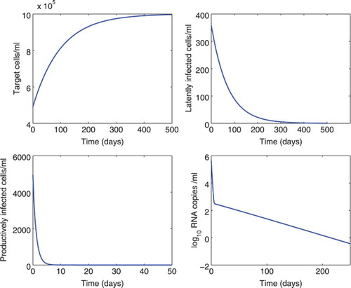
We chose the initial CD4+ T cell count $T\left(0\right)={10}^6$ cells per ml, initial viral load $V\left(0\right)={10}^{-3}$ virions per ml, $I\left(0\right)=0$, and $L\left(0\right)=0$. Numerical simulation of model (1(1) $\begin{array}{rl}\frac{\mathrm{d}T}{\mathrm{d}t}& =s-d_{T}T-\beta VT,\\ \frac{\mathrm{d}L}{\mathrm{d}t}& =f\beta V(t-{\tau }_1)T(t-{\tau }_1){\mathrm{e}}^{-{\delta }_1{\tau }_1}-{\delta }_{L}L-\alpha L,\\ \frac{\mathrm{d}I}{\mathrm{d}t}& =(1-f)\beta V(t-{\tau }_2)T(t-{\tau }_2){\mathrm{e}}^{-{\delta }_1{\tau }_2}-\delta I+\alpha L,\\ \frac{\mathrm{d}V}{\mathrm{d}t}& =N\delta I-cV.\end{array}$(1) ) shows that the solution approaches an infected steady state after some oscillations (Figure 1). The steady states of uninfected CD4+ T cells, latently infected cells, productively infected cells, and viral load are $4.92\times {10}^5$ cells per ml, 358.69 cells per ml, $4.96\times {10}^3$ cells per ml, and $4.31\times {10}^5$ viral RNA copies per ml, respectively. The basic reproductive number using the above parameter values is 2.03. According to the stability results, the infected steady state is globally asymptotically stable, which is illustrated by the numerical simulation shown in Figure 1.

Figure 1. Numerical simulation of model (1(1) $\begin{array}{rl}\frac{\mathrm{d}T}{\mathrm{d}t}& =s-d_{T}T-\beta VT,\\ \frac{\mathrm{d}L}{\mathrm{d}t}& =f\beta V(t-{\tau }_1)T(t-{\tau }_1){\mathrm{e}}^{-{\delta }_1{\tau }_1}-{\delta }_{L}L-\alpha L,\\ \frac{\mathrm{d}I}{\mathrm{d}t}& =(1-f)\beta V(t-{\tau }_2)T(t-{\tau }_2){\mathrm{e}}^{-{\delta }_1{\tau }_2}-\delta I+\alpha L,\\ \frac{\mathrm{d}V}{\mathrm{d}t}& =N\delta I-cV.\end{array}$(1) ) without treatment. The time delay ${\tau }_1$ was fixed to be 0.25 days and ${\tau }_2$ was fixed to be 0.5 days [45]. All the other parameter values are the same as those listed in Table 1.

In Figure 2, we showed the simulation of model (1(1) $\begin{array}{rl}\frac{\mathrm{d}T}{\mathrm{d}t}& =s-d_{T}T-\beta VT,\\ \frac{\mathrm{d}L}{\mathrm{d}t}& =f\beta V(t-{\tau }_1)T(t-{\tau }_1){\mathrm{e}}^{-{\delta }_1{\tau }_1}-{\delta }_{L}L-\alpha L,\\ \frac{\mathrm{d}I}{\mathrm{d}t}& =(1-f)\beta V(t-{\tau }_2)T(t-{\tau }_2){\mathrm{e}}^{-{\delta }_1{\tau }_2}-\delta I+\alpha L,\\ \frac{\mathrm{d}V}{\mathrm{d}t}& =N\delta I-cV.\end{array}$(1) ) under drug treatment. The overall drug efficacy was assumed to be 0.9, which means that the infection rate β is reduced by 90% [42]. Using the above steady states as the initial conditions of the model under treatment, the simulation shows that the CD4+ T cell level rebounds to the pre-infection level, and that all other infected cells and viral load decline to 0. In this case, the infection is predicted to die out. The effective reproductive number under treatment is 0.2. The simulation confirms the stability of the infection-free steady state when $R_0<1$.

Figure 2. Numerical simulation of model (1(1) $\begin{array}{rl}\frac{\mathrm{d}T}{\mathrm{d}t}& =s-d_{T}T-\beta VT,\\ \frac{\mathrm{d}L}{\mathrm{d}t}& =f\beta V(t-{\tau }_1)T(t-{\tau }_1){\mathrm{e}}^{-{\delta }_1{\tau }_1}-{\delta }_{L}L-\alpha L,\\ \frac{\mathrm{d}I}{\mathrm{d}t}& =(1-f)\beta V(t-{\tau }_2)T(t-{\tau }_2){\mathrm{e}}^{-{\delta }_1{\tau }_2}-\delta I+\alpha L,\\ \frac{\mathrm{d}V}{\mathrm{d}t}& =N\delta I-cV.\end{array}$(1) ) under treatment. The infection rate β was assumed to be reduced by 90%. The initial conditions were assumed to be the steady states of the model before treatment (see Figure 1). All the other parameter values are the same as those listed in Table 1.

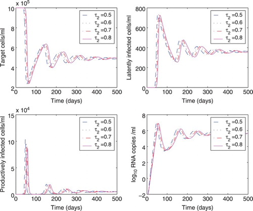
We also studied the effect of different time delays on the dynamics of model (1(1) $\begin{array}{rl}\frac{\mathrm{d}T}{\mathrm{d}t}& =s-d_{T}T-\beta VT,\\ \frac{\mathrm{d}L}{\mathrm{d}t}& =f\beta V(t-{\tau }_1)T(t-{\tau }_1){\mathrm{e}}^{-{\delta }_1{\tau }_1}-{\delta }_{L}L-\alpha L,\\ \frac{\mathrm{d}I}{\mathrm{d}t}& =(1-f)\beta V(t-{\tau }_2)T(t-{\tau }_2){\mathrm{e}}^{-{\delta }_1{\tau }_2}-\delta I+\alpha L,\\ \frac{\mathrm{d}V}{\mathrm{d}t}& =N\delta I-cV.\end{array}$(1) ) in Figures 3 and 4. In Figure 3, the delay ${\tau }_2$ was fixed to be 0.5 days and ${\tau }_1$ varied from 0.1 to 0.4 days. We found there is almost no difference in the dynamics of cells and viral load. In Figure 4, the delay ${\tau }_1$ was fixed to be 0.25 days and ${\tau }_2$ varied from 0.5 to 0.8 days. As the delay ${\tau }_2$ increases, there is a delay in the peak of target cells, infected cells, and viral load. However, there are very small differences in the steady states. This can be observed from the steady states shown in Equation (3(3) $\begin{array}{rl}{T}^{\ast }& =\frac{s}{d_T{R}_0},\\ L^{\ast }& =\frac{sf{\mathrm{e}}^{-{\delta }_1{\tau }_1}}{R_0({\delta }_L+\alpha )}(R_0-1),\\ I^{\ast }& =\frac{d_{T}c}{\beta N\delta }(R_0-1),\\ V^{\ast }& =\frac{d_T}{\beta }(R_0-1).\end{array}$(3) ) and the basic reproductive number shown in Equation (2(2) $R_0=\frac{s\beta N}{c{d}_T}\cdot \left[(1-f){\mathrm{e}}^{-{\delta }_1{\tau }_2}+\frac{\alpha }{{\delta }_L+\alpha }f{\mathrm{e}}^{-{\delta }_1{\tau }_1}\right].$(2) ).

Figure 3. Effect of different time delays (${\tau }_1$) on the dynamics of model (1(1) $\begin{array}{rl}\frac{\mathrm{d}T}{\mathrm{d}t}& =s-d_{T}T-\beta VT,\\ \frac{\mathrm{d}L}{\mathrm{d}t}& =f\beta V(t-{\tau }_1)T(t-{\tau }_1){\mathrm{e}}^{-{\delta }_1{\tau }_1}-{\delta }_{L}L-\alpha L,\\ \frac{\mathrm{d}I}{\mathrm{d}t}& =(1-f)\beta V(t-{\tau }_2)T(t-{\tau }_2){\mathrm{e}}^{-{\delta }_1{\tau }_2}-\delta I+\alpha L,\\ \frac{\mathrm{d}V}{\mathrm{d}t}& =N\delta I-cV.\end{array}$(1) ). The delay ${\tau }_1$ was chosen to be 0.1, 0.2, 0.3, or 0.4 days, and the delay ${\tau }_2$ was fixed at 0.5 days. All the other parameter values are the same as those in Figure 1. The lines of different cases overlap.

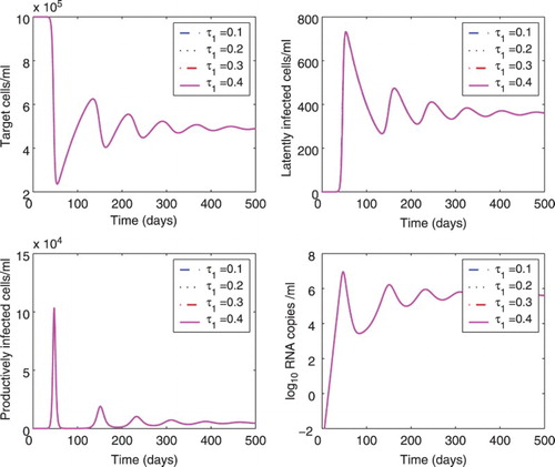
Figure 4. Effect of different time delays (${\tau }_2$) on the dynamics of model (1(1) $\begin{array}{rl}\frac{\mathrm{d}T}{\mathrm{d}t}& =s-d_{T}T-\beta VT,\\ \frac{\mathrm{d}L}{\mathrm{d}t}& =f\beta V(t-{\tau }_1)T(t-{\tau }_1){\mathrm{e}}^{-{\delta }_1{\tau }_1}-{\delta }_{L}L-\alpha L,\\ \frac{\mathrm{d}I}{\mathrm{d}t}& =(1-f)\beta V(t-{\tau }_2)T(t-{\tau }_2){\mathrm{e}}^{-{\delta }_1{\tau }_2}-\delta I+\alpha L,\\ \frac{\mathrm{d}V}{\mathrm{d}t}& =N\delta I-cV.\end{array}$(1) ). The delay ${\tau }_2$ was chosen to be 0.5, 0.6, 0.7, or 0.8 days, and the delay ${\tau }_1$ was fixed at 0.25 days. All the other parameter values are the same as those in Figure 1.

5. An HIV immune model with two delays

Pawelek et al. [33] studied a model of HIV infection with two time delays. One is the time (${\tau }_1$) needed for infected cells to produce virus after viral entry and the other is the time (${\tau }_2$) needed for the adaptive immune response to emerge to control viral replication. The model was fit to the viral load data from 10 patients during primary HIV infection. The model is described by the following system of differential equations. (16) $\begin{array}{rl}\frac{\mathrm{d}T}{\mathrm{d}t}& =s-d_{T}T-\beta VT,\\ \frac{\mathrm{d}I}{\mathrm{d}t}& ={\beta }_{1}V(t-{\tau }_1)T(t-{\tau }_1)-\delta I-d_{x}EI,\\ \frac{\mathrm{d}V}{\mathrm{d}t}& =N\delta I-cV,\\ \frac{\mathrm{d}E}{\mathrm{d}t}& =pI(t-{\tau }_2)-d_{E}E.\end{array}$(16) In the model, $E\left(t\right)$ is the concentration of effector cells at time t, which can kill productively infected cells. The variables T, I and V are the same as those in model (1(1) $\begin{array}{rl}\frac{\mathrm{d}T}{\mathrm{d}t}& =s-d_{T}T-\beta VT,\\ \frac{\mathrm{d}L}{\mathrm{d}t}& =f\beta V(t-{\tau }_1)T(t-{\tau }_1){\mathrm{e}}^{-{\delta }_1{\tau }_1}-{\delta }_{L}L-\alpha L,\\ \frac{\mathrm{d}I}{\mathrm{d}t}& =(1-f)\beta V(t-{\tau }_2)T(t-{\tau }_2){\mathrm{e}}^{-{\delta }_1{\tau }_2}-\delta I+\alpha L,\\ \frac{\mathrm{d}V}{\mathrm{d}t}& =N\delta I-cV.\end{array}$(1) ). The parameter β is the infection rate and ${\beta }_1=\beta {\mathrm{e}}^{-{\delta }_1{\tau }_1}$. The parameter $d_x$ is the killing rate of infected cells by effector cells, p is the generation rate of effector cells stimulated by productively infected cells, and $d_E$ is the death rate of effector cells. The other parameters are the same as those in model (1(1) $\begin{array}{rl}\frac{\mathrm{d}T}{\mathrm{d}t}& =s-d_{T}T-\beta VT,\\ \frac{\mathrm{d}L}{\mathrm{d}t}& =f\beta V(t-{\tau }_1)T(t-{\tau }_1){\mathrm{e}}^{-{\delta }_1{\tau }_1}-{\delta }_{L}L-\alpha L,\\ \frac{\mathrm{d}I}{\mathrm{d}t}& =(1-f)\beta V(t-{\tau }_2)T(t-{\tau }_2){\mathrm{e}}^{-{\delta }_1{\tau }_2}-\delta I+\alpha L,\\ \frac{\mathrm{d}V}{\mathrm{d}t}& =N\delta I-cV.\end{array}$(1) ). Parameters and values are also summarized in Table 1.

The model has two steady states: the infection-freesteady-state $E_0=(T_0,0,0,0)$ with $T_0=s/d_T$ and the infected steady-state $E_1=(\overline{T},\overline{I},\overline{V},\overline{E})$ where (17) $\begin{array}{rl}\overline{T}& =\frac{c^2{d}_{x}p}{2\beta {\beta }_1{N}^2{\delta }^2{d}_E}\left(\frac{\beta N{\delta }^2{d}_E}{c{d}_{x}p}-d_T+\sqrt{{\left(\frac{\beta N{\delta }^2{d}_E}{c{d}_{x}p}-d_T\right)}^2+4s\frac{\beta {\beta }_1{N}^2{\delta }^2{d}_E}{c^2{d}_{x}p}}\right),\\ \overline{I}& =\frac{d_E}{d_{x}p}\left(\frac{{\beta }_{1}N\delta \overline{T}}{c}-\delta \right),\\ \overline{V}& =\frac{N\delta }{c}\overline{I},\\ \overline{E}& =\frac{p}{d_E}\overline{I}.\end{array}$(17)

From $\overline{I}>0$, we know that the infected steady state exists if and only if ${\beta }_{1}N\overline{T}/c>1$, which is equivalent to ${\beta }_{1}Ns/\left(d_{T}c\right)>1$ or ${\beta }_{1}N{T}_0/c>1$. Note that $R_0={\beta }_{1}Ns/\left(d_{T}c\right)$ is the basic reproductive number of the basic model without the immune response [44].

It has been shown that for ${\tau }_1,{\tau }_2\ge 0$ the infection-free steady state is locally asymptotically stable when the basic reproductive number $R_0={\beta }_{1}Ns/\left(d_{T}c\right)<1$ [33]. The infected steady state is locally asymptotically stable when $R_0>1$ in the case of ${\tau }_2=0$. When ${\tau }_2>0$, the analysis of the stability of the infected steady state is challenging. Pawelek et al. [33] showed that even for a simplified model (assuming that the target cell level is constant $T=T_0=s/d_T$ in Equation (16(16) $\begin{array}{rl}\frac{\mathrm{d}T}{\mathrm{d}t}& =s-d_{T}T-\beta VT,\\ \frac{\mathrm{d}I}{\mathrm{d}t}& ={\beta }_{1}V(t-{\tau }_1)T(t-{\tau }_1)-\delta I-d_{x}EI,\\ \frac{\mathrm{d}V}{\mathrm{d}t}& =N\delta I-cV,\\ \frac{\mathrm{d}E}{\mathrm{d}t}& =pI(t-{\tau }_2)-d_{E}E.\end{array}$(16) )), a positive immune delay ${\tau }_2$ is able to destabilize the infected steady state. Specifically, in the case of ${\tau }_1=0$, it was shown that the infected steady state is locally asymptotically stable for ${\tau }_2<{\tau }_2^{\ast }$ and a Hopf bifurcation occurs when ${\tau }_2={\tau }_2^{\ast }$, where ${\tau }_2^{\ast }$ is a threshold value of the immune delay [33].

In this paper, we will investigate the case of ${\tau }_1>0$ and ${\tau }_2>0$. Because ${\delta }_1{\tau }_1$ is relatively small (i.e. ${\mathrm{e}}^{-{\delta }_1{\tau }_1}\approx 1$), we assume ${\beta }_1=\beta$ and consider the following simplified model. Stability crossing curves of the infected steady state will be explored for this model. (18) $\begin{array}{rl}\frac{\mathrm{d}I}{\mathrm{d}t}& =\beta V(t-{\tau }_1)T_0-\delta I-d_{x}EI,\\ \frac{\mathrm{d}V}{\mathrm{d}t}& =N\delta I-cV,\\ \frac{\mathrm{d}E}{\mathrm{d}t}& =pI(t-{\tau }_2)-d_{E}E.\end{array}$(18)

At the infected steady state, the characteristic equation of model (18(18) $\begin{array}{rl}\frac{\mathrm{d}I}{\mathrm{d}t}& =\beta V(t-{\tau }_1)T_0-\delta I-d_{x}EI,\\ \frac{\mathrm{d}V}{\mathrm{d}t}& =N\delta I-cV,\\ \frac{\mathrm{d}E}{\mathrm{d}t}& =pI(t-{\tau }_2)-d_{E}E.\end{array}$(18) ) is (19) $(\lambda +c)\left[\right(\lambda +R_0\delta \left)\right(\lambda +d_E)+(R_0-1\left)d_E\delta {\mathrm{e}}^{-\lambda {\tau }_2}\right]=(\lambda +d_E)R_{0}c\delta {\mathrm{e}}^{-\lambda {\tau }_1},$(19) where λ is the eigenvalue and $R_0=\beta N{T}_0/c=\beta Ns/c{d}_T$. Expanding the product, the above equation can be written as the following equation $p_0\left(\lambda \right)+p_1\left(\lambda \right){\mathrm{e}}^{-{\tau }_1\lambda }+p_2\left(\lambda \right){\mathrm{e}}^{-{\tau }_2\lambda }=0,$ where (20) $\begin{array}{rl}{p}_0\left(\lambda \right)& ={\lambda }^3+(R_0\delta +d_E+c){\lambda }^2+[d_E{R}_0\delta +c(R_0\delta +d_E\left)\right]\lambda +c{d}_E{R}_0\delta ,\\ p_1\left(\lambda \right)& =-R_{0}c\delta \lambda -d_E{R}_{0}c\delta ,\\ p_2\left(\lambda \right)& =(R_0-1)d_E\delta \lambda +c(R_0-1)d_E\delta .\end{array}$(20) Thus, the stability of the infected steady state is determined by the zeros of the characteristic quasipolynomial $p(\lambda ,{\tau }_1,{\tau }_2)=p_0\left(\lambda \right)+p_1\left(\lambda \right){\mathrm{e}}^{-{\tau }_1\lambda }+p_2\left(\lambda \right){\mathrm{e}}^{-{\tau }_2\lambda }.$ The main objective of the remaining part of this section is to identify the stability crossing curves of $({\tau }_1,{\tau }_2)$ in ${\mathbb{R}}_{+}^2$ (i.e. the set of two-dimensional vectors with non-negative components).

We start with the definition of stability crossing curve, which was used in Gu et al. [16].

Definition 5.1.

The stability crossing curve $\mathcal{T}$ is the set of all crossing points $({\tau }_1,{\tau }_2)$ in ${\mathbb{R}}_{+}^2,$ where $({\tau }_1,{\tau }_2)$ is the point such that $p(\lambda ,{\tau }_1,{\tau }_2)$ has at least one zero on the imaginary axis. Thus, $\mathcal{T}$ can be written as $\mathcal{T}=\left\{\right({\tau }_1,{\tau }_2):p(\lambda ,{\tau }_1,{\tau }_2)=0\text{for some}\lambda =j\omega \}$.

From Equation (20(20) $\begin{array}{rl}{p}_0\left(\lambda \right)& ={\lambda }^3+(R_0\delta +d_E+c){\lambda }^2+[d_E{R}_0\delta +c(R_0\delta +d_E\left)\right]\lambda +c{d}_E{R}_0\delta ,\\ p_1\left(\lambda \right)& =-R_{0}c\delta \lambda -d_E{R}_{0}c\delta ,\\ p_2\left(\lambda \right)& =(R_0-1)d_E\delta \lambda +c(R_0-1)d_E\delta .\end{array}$(20) ), it is easy to show that $p_0\left(\lambda \right)$ does not have zeros on the imaginary axis. Let $a(\lambda ,{\tau }_1,{\tau }_2)=p(\lambda ,{\tau }_1,{\tau }_2)/p_0\left(\lambda \right)$. We have $a(\lambda ,{\tau }_1,{\tau }_2)=1+a_1\left(\lambda \right){\mathrm{e}}^{-{\tau }_1\lambda }+a_2\left(\lambda \right){\mathrm{e}}^{-{\tau }_2\lambda }$, where $a_1\left(\lambda \right)=p_1\left(\lambda \right)/p_0\left(\lambda \right)$ and $a_2\left(\lambda \right)=p_2\left(\lambda \right)/p_0\left(\lambda \right)$. Thus, for given ${\tau }_1$ and ${\tau }_2$, $p(\lambda ,{\tau }_1,{\tau }_2)$ and $a(\lambda ,{\tau }_1,{\tau }_2)$ have the same zeros in a neighbourhood of the imaginary axis. Instead of using $p(\lambda ,{\tau }_1,{\tau }_2)=0$, we will study the crossing points from the solutions of the following equation (21) $a(\lambda ,{\tau }_1,{\tau }_2)=1+a_1\left(\lambda \right){\mathrm{e}}^{-{\tau }_1\lambda }+a_2\left(\lambda \right){\mathrm{e}}^{-{\tau }_2\lambda }=0.$(21)

From Equation (20(20) $\begin{array}{rl}{p}_0\left(\lambda \right)& ={\lambda }^3+(R_0\delta +d_E+c){\lambda }^2+[d_E{R}_0\delta +c(R_0\delta +d_E\left)\right]\lambda +c{d}_E{R}_0\delta ,\\ p_1\left(\lambda \right)& =-R_{0}c\delta \lambda -d_E{R}_{0}c\delta ,\\ p_2\left(\lambda \right)& =(R_0-1)d_E\delta \lambda +c(R_0-1)d_E\delta .\end{array}$(20) ), we have that for model (18(18) $\begin{array}{rl}\frac{\mathrm{d}I}{\mathrm{d}t}& =\beta V(t-{\tau }_1)T_0-\delta I-d_{x}EI,\\ \frac{\mathrm{d}V}{\mathrm{d}t}& =N\delta I-cV,\\ \frac{\mathrm{d}E}{\mathrm{d}t}& =pI(t-{\tau }_2)-d_{E}E.\end{array}$(18) ) (22) $a_1\left(\lambda \right)=\frac{-R_{0}c\delta \lambda -d_E{R}_{0}c\delta }{{\lambda }^3+(R_0\delta +d_E+c){\lambda }^2+[d_E{R}_0\delta +c(R_0\delta +d_E\left)\right]\lambda +c{d}_E{R}_0\delta },$(22) and (23) $a_2\left(\lambda \right)=\frac{(R_0-1)d_E\delta \lambda +c(R_0-1)d_E\delta }{{\lambda }^3+(R_0\delta +d_E+c){\lambda }^2+[d_E{R}_0\delta +c(R_0\delta +d_E\left)\right]\lambda +c{d}_E{R}_0\delta }.$(23)

Next, we recall a few propositions that can be used to characterize the stability crossing curves of a general linear scalar system with two time delays. The proof of these propositions can be found in Gu et al. [16].

Proposition 5.2.

For each $\omega ,\omega \ne 0,$ $p_0\left(j\omega \right)\ne 0,$ $\lambda =j\omega$ can be a solution of $p(\lambda ,{\tau }_1,{\tau }_2)=0$ for some $({\tau }_1,{\tau }_2)\in {\mathbb{R}}_{+}^2$ if and only if (24) $\begin{array}{r}|a_1\left(j\omega \right)|+|a_2\left(j\omega \right)|\ge 1,\end{array}$(24) (25) $\begin{array}{r}-1\le |a_1\left(j\omega \right)|-|a_2\left(j\omega \right)|\le 1.\end{array}$(25) For $\omega \ne 0$ satisfying $p_0\left(j\omega \right)=0,\lambda =j\omega$ can be zero of $p(\lambda ,{\tau }_1,{\tau }_2)$ for some $({\tau }_1,{\tau }_2)\in {\mathbb{R}}_{+}^2$ if and only if $|p_1\left(j\omega \right)|=|p_2\left(j\omega \right)|.$

For our model (18(18) $\begin{array}{rl}\frac{\mathrm{d}I}{\mathrm{d}t}& =\beta V(t-{\tau }_1)T_0-\delta I-d_{x}EI,\\ \frac{\mathrm{d}V}{\mathrm{d}t}& =N\delta I-cV,\\ \frac{\mathrm{d}E}{\mathrm{d}t}& =pI(t-{\tau }_2)-d_{E}E.\end{array}$(18) ), $p_0\left(j\omega \right)$ cannot be 0 for any $\omega \ne 0$. Thus, $\lambda =j\omega$ is a solution of $p(\lambda ,{\tau }_1,{\tau }_2)$ for some $({\tau }_1,{\tau }_2)\in {\mathbb{R}}_{+}^2$ if and only if $a_1\left(j\omega \right)$ and $a_2\left(j\omega \right)$ satisfy inequalities (24(24) $\begin{array}{r}|a_1\left(j\omega \right)|+|a_2\left(j\omega \right)|\ge 1,\end{array}$(24) ) and (25(25) $\begin{array}{r}-1\le |a_1\left(j\omega \right)|-|a_2\left(j\omega \right)|\le 1.\end{array}$(25) ).

We define the crossing set Ω as the set of all $\omega >0$ that satisfy Equations (24(24) $\begin{array}{r}|a_1\left(j\omega \right)|+|a_2\left(j\omega \right)|\ge 1,\end{array}$(24) ) and (25(25) $\begin{array}{r}-1\le |a_1\left(j\omega \right)|-|a_2\left(j\omega \right)|\le 1.\end{array}$(25) ). From Proposition 5.2, we have $\mathrm{\Omega }=\{\omega :p(j\omega ,{\tau }_1,{\tau }_2)=0\mathrm{forsome}({\tau }_1,{\tau }_2\left)\right\}$. Furthermore, all the pairs of $({\tau }_1,{\tau }_2)$ satisfying Equation (21(21) $a(\lambda ,{\tau }_1,{\tau }_2)=1+a_1\left(\lambda \right){\mathrm{e}}^{-{\tau }_1\lambda }+a_2\left(\lambda \right){\mathrm{e}}^{-{\tau }_2\lambda }=0.$(21) ) can be calculated as follows [16]: (26) $\begin{array}{rl}{\tau }_1& ={\tau }_1^{u\pm }\left(\omega \right)=\frac{\mathrm{\angle }{a}_1\left(j\omega \right)+(2u-1)\pi \pm {\theta }_1}{\omega }\ge 0,u=u_0^{\pm },u_0^{\pm }+1,u_0^{\pm }+2,\dots ,\end{array}$(26) (27) $\begin{array}{rl}{\tau }_2& ={\tau }_2^{v\pm }\left(\omega \right)=\frac{\mathrm{\angle }{a}_2\left(j\omega \right)+(2v-1)\pi \pm {\theta }_2}{\omega }\ge 0,v=v_0^{\pm },v_0^{\pm }+1,v_0^{\pm }+2,\dots ,\end{array}$(27) where ∠ represents the argument of a complex number, ${\theta }_1,{\theta }_2\in [0,\pi ]$ are given by (28) $\begin{array}{rl}{\theta }_1& ={\cos }^{-1}\left(\frac{1+|a_1\left(j\omega \right){|}^2-|a_2\left(j\omega \right){|}^2-|a_2\left(j\omega \right){|}^2}{2|a_1\left(j\omega \right)|}\right),\end{array}$(28) (29) $\begin{array}{rl}{\theta }_2& ={\cos }^{-1}\left(\frac{1+|a_2\left(j\omega \right){|}^2-|a_1\left(j\omega \right){|}^2-|a_1\left(j\omega \right){|}^2}{2|a_1\left(j\omega \right)|}\right),\end{array}$(29) and $u_0^{+}$, $u_0^{-}$, $v_0^{+}$, $v_0^{-}$ are the smallest possible integers such that the corresponding ${\tau }_1^{u_0^{+}+},{\tau }_1^{u_0^{-}-},{\tau }_2^{v_0^{+}+},{\tau }_2^{v_0^{-}-}$ calculated are non-negative. Note that $({\tau }_1^{u+},{\tau }_2^{v+})$ and $({\tau }_1^{u-},{\tau }_2^{v-})$ are mirror images with respect to the real axis.

The following result regarding the crossing set Ω was obtained in ref. [16].

Proposition 5.3.

The crossing set Ω consists of a finite number of intervals of finite length.

Let these intervals be ${\mathrm{\Omega }}_k$, $k=1,2,\dots ,N$, which are arranged in an order such that the left-end point of ${\mathrm{\Omega }}_k$ increases with increasing k. Then $\mathrm{\Omega }=\bigcup _{k=1}^N{\mathrm{\Omega }}_k$.

Let $\begin{array}{rl}{\mathcal{T}}_{u,v}^{\pm k}& =\bigcup _{\omega \in {\mathrm{\Omega }}_k}{\mathcal{T}}_{\omega ,u,v}^{\pm }=\left\{\right({\tau }_1^{u\pm }\left(\omega \right),{\tau }_2^{v\pm }\left(\omega \right))|\omega \in {\mathrm{\Omega }}_k\},\\ {\mathcal{T}}^k& =\bigcup _{u=-\mathrm{\infty }}^{\mathrm{\infty }}\bigcup _{v=-\mathrm{\infty }}^{\mathrm{\infty }}({\mathcal{T}}_{u,v}^{+k}\cup {\mathcal{T}}_{u,v}^{-k})\cap {\mathbb{R}}_{+}^2=\bigcup _{\omega \in {\mathrm{\Omega }}_k}{\mathcal{T}}_{\omega }.\end{array}$ The stability crossing curves $\mathcal{T}$ can be written as the union of ${\mathcal{T}}^k$, $k=1,\dots ,N$, that is, $\mathcal{T}=\bigcup _{k=1}^N{\mathcal{T}}^k$.

Let ${\mathrm{\Omega }}_k=[{\omega }_k^l,{\omega }_k^r]$, $k=1,\dots ,N$, where ${\omega }_k^l$ and ${\omega }_k^r$ are the left and right end points, respectively. The end points of the intervals ${\mathrm{\Omega }}_k$, $k=1,\dots ,N$, can be classified into the following three types (Type 1, Type 2, and Type 3). Type 0 is an additional type if the left-end point is equal to 0 [16].

Type 1. $|a_1\left(j\omega \right)|-|a_2\left(j\omega \right)|=1$ is satisfied. In this case, ${\theta }_1=0,{\theta }_2=\pi$, and ${\mathcal{T}}_{u,v}^{+k}$ is connected with ${\mathcal{T}}_{u,v-1}^{-k}$ at this end.

Type 2. $|a_2\left(j\omega \right)|-|a_1\left(j\omega \right)|=1$ is satisfied. In this case, ${\theta }_1=\pi ,{\theta }_2=0$, and ${\mathcal{T}}_{u,v}^{+k}$ is connected with ${\mathcal{T}}_{u+1,v}^{-k}$ at this end.

Type 3. $|a_1\left(j\omega \right)|+|a_2\left(j\omega \right)|=1$ is satisfied. In this case, ${\theta }_1={\theta }_2=0$, and ${\mathcal{T}}_{u,v}^{+k}$ is connected with ${\mathcal{T}}_{u,v}^{-k}$ at this end.

Type 0. ${\omega }_k^l$ is equal to 0. In this case, $\omega =0$ satisfies Equations (24(24) $\begin{array}{r}|a_1\left(j\omega \right)|+|a_2\left(j\omega \right)|\ge 1,\end{array}$(24) ) and (25(25) $\begin{array}{r}-1\le |a_1\left(j\omega \right)|-|a_2\left(j\omega \right)|\le 1.\end{array}$(25) ). As $\omega \to 0$, ${\mathcal{T}}_{u,v}^{+k}$ and ${\mathcal{T}}_{u,v}^{-k}$ approach ∞ with asymptotes passing through the points $({\hat{a}}_1\pm {\hat{\theta }}_1,{\hat{a}}_2\pm {\hat{\theta }}_2)$ with slopes of (30) $\frac{{\tau }_2^{v\pm }}{{\tau }_1^{u\pm }}\to {\kappa }_{u,v}^{\pm }=\frac{\mathrm{\angle }{a}_2\left(0\right)+(2v-1)\pi \pm {\theta }_2\left(0\right)}{\mathrm{\angle }{a}_1\left(0\right)+(2u-1)\pi \pm {\theta }_1\left(0\right)},$(30) where ${\theta }_1\left(0\right)$ and ${\theta }_2\left(0\right)$ are evaluated by Equations (28(28) $\begin{array}{rl}{\theta }_1& ={\cos }^{-1}\left(\frac{1+|a_1\left(j\omega \right){|}^2-|a_2\left(j\omega \right){|}^2-|a_2\left(j\omega \right){|}^2}{2|a_1\left(j\omega \right)|}\right),\end{array}$(28) ) and (29(29) $\begin{array}{rl}{\theta }_2& ={\cos }^{-1}\left(\frac{1+|a_2\left(j\omega \right){|}^2-|a_1\left(j\omega \right){|}^2-|a_1\left(j\omega \right){|}^2}{2|a_1\left(j\omega \right)|}\right),\end{array}$(29) ) using $a_1\left(0\right)$ and $a_2\left(0\right)$, respectively, and ${\hat{a}}_l=\frac{d}{d\omega }\left[\mathrm{\angle }{a}_l\right(j\omega ){]}_{\omega =0},{\hat{\theta }}_l=\frac{d}{d\omega }{\hat{\theta }}_l(j\omega ){|}_{w=0},\text{for}l=1,2.$

An interval ${\mathrm{\Omega }}_k$ of the crossing set Ω is said to be of type lr if the left-end point of ${\mathrm{\Omega }}_k$ is of type l and the right-end point is of type r.

It follows from Equations (22(22) $a_1\left(\lambda \right)=\frac{-R_{0}c\delta \lambda -d_E{R}_{0}c\delta }{{\lambda }^3+(R_0\delta +d_E+c){\lambda }^2+[d_E{R}_0\delta +c(R_0\delta +d_E\left)\right]\lambda +c{d}_E{R}_0\delta },$(22) ) and (23(23) $a_2\left(\lambda \right)=\frac{(R_0-1)d_E\delta \lambda +c(R_0-1)d_E\delta }{{\lambda }^3+(R_0\delta +d_E+c){\lambda }^2+[d_E{R}_0\delta +c(R_0\delta +d_E\left)\right]\lambda +c{d}_E{R}_0\delta }.$(23) ) that $a_1\left(0\right)=-1$ and $a_2\left(0\right)=1-1/R_0$. Because of $R_0>1$, we have $|a_1\left(0\right)|-|a_2\left(0\right)|=1/R_0\in (0,1)$ and $|a_1\left(0\right)|+|a_2\left(0\right)|=2-1/R_0\in (1,2)$. Thus, $\omega =0$ satisfies Equations (24(24) $\begin{array}{r}|a_1\left(j\omega \right)|+|a_2\left(j\omega \right)|\ge 1,\end{array}$(24) ) and (25(25) $\begin{array}{r}-1\le |a_1\left(j\omega \right)|-|a_2\left(j\omega \right)|\le 1.\end{array}$(25) ), which means that 0 is the left-end point of the interval ${\mathrm{\Omega }}_1$, belonging to type 0. From Equations (22(22) $a_1\left(\lambda \right)=\frac{-R_{0}c\delta \lambda -d_E{R}_{0}c\delta }{{\lambda }^3+(R_0\delta +d_E+c){\lambda }^2+[d_E{R}_0\delta +c(R_0\delta +d_E\left)\right]\lambda +c{d}_E{R}_0\delta },$(22) ) and (23(23) $a_2\left(\lambda \right)=\frac{(R_0-1)d_E\delta \lambda +c(R_0-1)d_E\delta }{{\lambda }^3+(R_0\delta +d_E+c){\lambda }^2+[d_E{R}_0\delta +c(R_0\delta +d_E\left)\right]\lambda +c{d}_E{R}_0\delta }.$(23) ), it is also easy to show that $\underset{\omega \to \mathrm{\infty }}{lim}|a_1\left(j\omega \right)|-|a_2\left(j\omega \right)|=|a_1\left(j\omega \right)|+|a_2\left(j\omega \right)|=0.$ Thus, there is at least one solution ω of the equation $|a_1\left(j\omega \right)|+|a_2\left(j\omega \right)|=1$.

In the upper panel of Figure 5, we plotted $|a_1\left(j\omega \right)|-|a_2\left(j\omega \right)|$ (solid curve) and $|a_1\left(j\omega \right)|+|a_2\left(j\omega \right)|$ (dashed curve), respectively, as a function of ω. The basic reproductive number was chosen to be $R_0=2.6$, the death rate of infected cells was set to $\delta =0.3$ day⁻¹, the viral clearance rate was chosen to be c=23 day⁻¹, and the death rate of effector cells was chosen to be $d_E=0.45$ day⁻¹. These parameter values were chosen based on the fitting of the two-delay model (Equation 16(16) $\begin{array}{rl}\frac{\mathrm{d}T}{\mathrm{d}t}& =s-d_{T}T-\beta VT,\\ \frac{\mathrm{d}I}{\mathrm{d}t}& ={\beta }_{1}V(t-{\tau }_1)T(t-{\tau }_1)-\delta I-d_{x}EI,\\ \frac{\mathrm{d}V}{\mathrm{d}t}& =N\delta I-cV,\\ \frac{\mathrm{d}E}{\mathrm{d}t}& =pI(t-{\tau }_2)-d_{E}E.\end{array}$(16) ) to the data from 10 patients during primary infection [33]. We found there is only one intersection point $\omega =0.69$ between $|a_1\left(j\omega \right)|+|a_2\left(j\omega \right)|$ and y=1. Therefore, there is only one interval ${\mathrm{\Omega }}_1=(0,0.69]$ in the crossing set Ω, which is of type 03. Corresponding to ${\mathrm{\Omega }}_1$, there are only one type of stability crossing curves ${\mathcal{T}}^1$. Furthermore, for type 03, ${\mathcal{T}}_{u,v}^{+1}$ and ${\mathcal{T}}_{u,v}^{-1}$ are connected at the left-end point ${\omega }_1^r=0$. The other ends of ${\mathcal{T}}_{u,v}^{+1}$ and ${\mathcal{T}}_{u,v}^{-1}$ extend to infinity with slopes $k_{u,v}^{+}$ and $k_{u,v}^{-}$ (given in Equation (30(30) $\frac{{\tau }_2^{v\pm }}{{\tau }_1^{u\pm }}\to {\kappa }_{u,v}^{\pm }=\frac{\mathrm{\angle }{a}_2\left(0\right)+(2v-1)\pi \pm {\theta }_2\left(0\right)}{\mathrm{\angle }{a}_1\left(0\right)+(2u-1)\pi \pm {\theta }_1\left(0\right)},$(30) )), respectively. Therefore, ${\mathcal{T}}^1$ consists of a series of open-ended curves with both ends approaching ∞. These open-ended curves in ${\mathbb{R}}_{+}^2$ were plotted in the lower panel of Figure 5 for the infected steady state of model (18(18) $\begin{array}{rl}\frac{\mathrm{d}I}{\mathrm{d}t}& =\beta V(t-{\tau }_1)T_0-\delta I-d_{x}EI,\\ \frac{\mathrm{d}V}{\mathrm{d}t}& =N\delta I-cV,\\ \frac{\mathrm{d}E}{\mathrm{d}t}& =pI(t-{\tau }_2)-d_{E}E.\end{array}$(18) ).

Figure 5. Upper panel: plots of $|a_1\left(j\omega \right)|\pm |a_2\left(j\omega \right)|$ (see Equations (22(22) $a_1\left(\lambda \right)=\frac{-R_{0}c\delta \lambda -d_E{R}_{0}c\delta }{{\lambda }^3+(R_0\delta +d_E+c){\lambda }^2+[d_E{R}_0\delta +c(R_0\delta +d_E\left)\right]\lambda +c{d}_E{R}_0\delta },$(22) ) and (23(23) $a_2\left(\lambda \right)=\frac{(R_0-1)d_E\delta \lambda +c(R_0-1)d_E\delta }{{\lambda }^3+(R_0\delta +d_E+c){\lambda }^2+[d_E{R}_0\delta +c(R_0\delta +d_E\left)\right]\lambda +c{d}_E{R}_0\delta }.$(23) )) as a function of ω. The intersection point of $|a_1\left(j\omega \right)|+|a_2\left(j\omega \right)|$ and 1 is 0.69. Lower panel: stability crossing curves corresponding to the crossing interval (0, 0.69] for the two-delay model (18(18) $\begin{array}{rl}\frac{\mathrm{d}I}{\mathrm{d}t}& =\beta V(t-{\tau }_1)T_0-\delta I-d_{x}EI,\\ \frac{\mathrm{d}V}{\mathrm{d}t}& =N\delta I-cV,\\ \frac{\mathrm{d}E}{\mathrm{d}t}& =pI(t-{\tau }_2)-d_{E}E.\end{array}$(18) ). The basic reproductive number was chosen to be $R_0=2.6$. The other parameters were chosen based on the estimates from data fitting in ref. [33]: $\delta =0.3$ day⁻¹, c=23 day⁻¹, and $d_E=0.45$ day⁻¹.

The upper panel of Figure 6 showed the changes of $|a_1\left(j\omega \right)|-|a_2\left(j\omega \right)|$ and $|a_1\left(j\omega \right)|+|a_2\left(j\omega \right)|$ when the basic reproductive number was chosen to be $R_0=5$. The other parameter values are the same as those in Figure 5. There is again only one solution $\omega =1.12$ of the equation $|a_1\left(j\omega \right)|+|a_2\left(j\omega \right)|=1$. Thus, there is only one crossing interval ${\mathrm{\Omega }}_1=(0,1.12]$, which is of type 03. The open-ended stability crossing curves corresponding to this interval were shown in the lower panel of Figure 6.

6. Conclusion and discussion

This paper investigates the asymptotical behaviour of the solutions of delay differential equation systems that are used to study HIV infection dynamics. The first model was used to determine the contribution of latently infected cell activation to HIV production during combination antiretroviral therapy [38]. We incorporated two delays into the model. One is the time between initial cell infection and the establishment of latent infection, and the other is the time between viral entry into cell and viral production in productively infected cells. Although the second delay was included to evaluate its influence on HIV dynamics and parameter estimates in the literature [18, 27–29], the first time delay has not been studied before. We derived the basic reproductive number and performed both local and global stability analysis of the steady states. We showed that the infection-free steady state is globally asymptotically stable when the basic reproductive number is less than 1, and the infected steady state is globally asymptotically stable when the basic reproductive number is greater than 1. Thus, incorporation of the latent infection delay does not destabilize the stability of the steady state. This is consistent with the results of models including intracellular delay [22, 23]. Numerical results also confirm the stability analysis. Simulation of the model with different delays shows that the delay between viral entry and viral integration has a very minor effect on the dynamics of cells and viral load. The time delay between viral infection and viral production causes a very small change in the steady states of infected cells and viral load, but postpones the time to reach the viral peak.

Figure 6. Upper panel: plots of $|a_1\left(j\omega \right)|\pm |a_2\left(j\omega \right)|$ as a function of ω. The intersection point of $|a_1\left(j\omega \right)|+|a_2\left(j\omega \right)|$ and 1 is 1.12. Lower panel: stability crossing curves corresponding to the crossing interval (0, 1.12] for the two-delay model (18(18) $\begin{array}{rl}\frac{\mathrm{d}I}{\mathrm{d}t}& =\beta V(t-{\tau }_1)T_0-\delta I-d_{x}EI,\\ \frac{\mathrm{d}V}{\mathrm{d}t}& =N\delta I-cV,\\ \frac{\mathrm{d}E}{\mathrm{d}t}& =pI(t-{\tau }_2)-d_{E}E.\end{array}$(18) ). The basic reproductive number was chosen to be $R_0=5$. The other parameters are the same as those in Figure 5.

The model analysis suggests if treatment is very effective then the basic reproductive number will become less than 1, and both the latent reservoir and the virus are predicted to die out. However, current treatment consisting of several antiretroviral drugs cannot eradicate the latent reservoir (and the virus). One reason may be that current treatment regimens are not sufficiently effective to block all the infection and thus there exists residual ongoing viral replication [40]. Another reason is the intrinsic stability of latently infected CD4+ T cells [4]. Some explanations such as asymmetric cell division [42], programmed expansion and contraction [41], and homeostatic proliferation [41] of latently infected cells have been proposed and tested by mathematical models. Homeostatic proliferation has been experimentally confirmed [6]. Some other models studying the dynamics of the latent reservoir and low-level viral load persistence during effective antiretroviral therapy can be found in refs. [2, 14, 48, 50] and references cited therein. Reviews of mathematical models and implications for treatment can be found in refs. [36, 43].

The second model also includes two delays. One is the time needed for infected cells to produce virus following cell infection (i.e. ${\tau }_1$, the intracellular delay), and the other is the time needed for the CD8+ T cell response to emerge to control viral replication (i.e. ${\tau }_2$, the immune delay). Some special cases of the immune model with two delays have been investigated in a previous study [33]. However, the analysis of the model with two positive delays is challenging. We showed that introducing the intracellular delay does not change the stability results but including the immune delay in the model generates rich dynamics. A Hopf bifurcation was shown to take place at a critical threshold of the immune delay for a simplified model assuming that the target cell level is constant [33]. When the two delays are both positive, the stability crossing curves of the HIV immune model have not been characterized. Several papers in the literature have studied the properties of the solutions of models with two delays for different problems [1, 9, 19, 24, 30, 46, 47]. Gu et al. investigated a general linear scalar system with two delays and showed that the stability crossing curves fall into three categories of curves, namely, closed curves, open-ended curves, and spiral-like curves oriented horizontally, vertically, or diagonally [16]. We applied the method to the characteristic quasipolynomial for the HIV immune model, and found that the stability crossing curves consist of a series of open-ended curves in the delay-parameter space. Overall, this analysis helps to better understand the dynamical behaviour of HIV models with two time delays.

Acknowledgments

The authors would like to thank Professor Keqin Gu for providing help in the simulation of the stability crossing curves. The work was finished when X. Wang visited Oakland University in 2015.

Disclosure statement

No potential conflict of interest was reported by the authors.

Additional information

Funding

X. Wang is supported by the NNSF of China (No.11301453), Postdoctoral Science Foundation of China (2014M562366), Postdoctoral Science Foundation of Shaanxi Province (2014010), the Universities Young Teachers Program of Henan Province (2014GGJS-093), and Doctoral Scientific Research Startup Fund of Xinyang Normal University (2014033). L. Rong is supported by the NSF grants DMS 1122290 and 1349939.

References

- M. Adimy, F. Crauste, and S. Ruan, Periodic oscillations in leukopoiesis models with two delays, J. Theoret. Biol. 242 (2006), pp. 288–299. doi: 10.1016/j.jtbi.2006.02.020
- N.M. Archin, N.K. Vaidya, J.D. Kuruc, A.L. Liberty, A. Wiegand, M.F. Kearney, M.S. Cohen, J.M. Coffin, R.J. Bosch, C.L. Gay, J.J. Eron, D.M. Margolis, and A.S. Perelson, Immediate antiviral therapy appears to restrict resting CD4+ cell HIV-1 infection without accelerating the decay of latent infection, Proc. Natl. Acad. Sci. USA 109 (2012), pp. 9523–9528. doi: 10.1073/pnas.1120248109
- H.T. Banks, D.M. Bortz, and S.E. Holte, Incorporation of variability into the modeling of viral delays in HIV infection dynamics, Math. Biosci. 183 (2003), pp. 63–91. doi: 10.1016/S0025-5564(02)00218-3
- J.N. Blankson, D. Persaud, and R.F. Siliciano, The challenge of viral reservoirs in HIV-1 infection, Annu. Rev. Med. 53 (2002), pp. 557–593. doi: 10.1146/annurev.med.53.082901.104024
- M. Bofill, G. Janossy, C.A. Lee, D. MacDonald-Burns, A.N. Phillips, C. Sabin, A. Timms, M.A. Johnson, and P.B. Kernoff, Laboratory control values for CD4 and CD8 T lymphocytes: Implications for HIV-1 diagnosis, Clin. Exp. Immunol. 88 (1992), pp. 243–252. doi: 10.1111/j.1365-2249.1992.tb03068.x
- N. Chomont, M. El-Far, P. Ancuta, L. Trautmann, F.A. Procopio, B. Yassine-Diab, G. Boucher, M.-R. Boulassel, G. Ghattas, J.M. Brenchley, T.W. Schacker, B.J. Hill, D.C. Douek, J.-P. Routy, E.K. Haddad, and R.-P. Sékaly, HIV reservoir size and persistence are driven by T cell survival and homeostatic proliferation, Nat. Med. 15 (2009), pp. 893–900. doi: 10.1038/nm.1972
- T. -W. Chun, L. Stuyver, S.B. Mizell, L.A. Ehler, J.A.M. Mican, M. Baseler, A.L. Lloyd, M.A. Nowak, and A.S. Fauci, Presence of an inducible HIV-1 latent reservoir during highly active antiretroviral therapy, Proc. Natl. Acad. Sci. USA 94 (1997), pp. 13193–13197. doi: 10.1073/pnas.94.24.13193
- M.S. Ciupe, B.L. Bivort, D.M. Bortz, and P.W. Nelson, Estimating kinetic parameters from HIV primary infection data through the eyes of three different mathematical models, Math. Biosci. 200 (2006), pp. 1–27. doi: 10.1016/j.mbs.2005.12.006
- K.L. Cooke and P. van den Driessche, Analysis of an SEIRS epidemic model with two delays, J. Math. Biol. 35 (1996), pp. 240–260. doi: 10.1007/s002850050051
- S.M. Crowe, J.B. Carlin, K.I. Stewart, C.R. Lucas, and J.F. Hoy, Predictive value of CD4 lymphocyte numbers for the development of opportunistic infections and malignancies in HIV-infected persons, J. Acquir. Immune Defic. Syndr. 4 (1991), pp. 770–776.
- R.V. Culshaw, S. Ruan, and G. Webb, A mathematical model of cell-to-cell spread of HIV-1 that includes a time delay, J. Math. Biol. 46 (2003), pp. 425–444. doi: 10.1007/s00285-002-0191-5
- N.M. Dixit and A.S. Perelson, Complex patterns of viral load decay under antiretroviral therapy: Influence of pharmacokinetics and intracellular delay, J. Theoret. Biol. 226 (2004), pp. 95–109. doi: 10.1016/j.jtbi.2003.09.002
- D. Finzi, M. Hermankova, T. Pierson, L.M. Carruth, C. Buck, R.E. Chaisson, T.C. Quinn, K. Chadwick, J. Margolick, R. Brookmeyer, J. Gallant, M. Markowitz, D.D. Ho, D.D. Richman, and R.F. Siliciano, Identification of a reservoir for HIV-1 in patients on highly active antiretroviral therapy, Science 278 (1997), pp. 1295–1300. doi: 10.1126/science.278.5341.1295
- J. Forde, J.M. Volpe, and S.M. Ciupe, Latently infected cell activation: A way to reduce the size of the HIV reservoir? Bull. Math. Biol. 74 (2012), pp. 1651–1672. doi: 10.1007/s11538-012-9729-x
- Z. Grossman, M. Polis, M.B. Feinberg, Z. Grossman, I. Levi, S. Jankelevich, R. Yarchoan, J. Boon, F. de Wolf, J.M.A. Lange, J. Goudsmit, D.S. Dimitrov, and W.E. Paul, Ongoing HIV dissemination during HAART, Nat. Med. 5 (1999), pp. 1099–1104. doi: 10.1038/13410
- K. Gu, S. -I. Niculescu, and J. Chen, On stability crossing curves for general systems with two delays, J. Math. Anal. Appl. 311 (2005), pp. 231–253. doi: 10.1016/j.jmaa.2005.02.034
- J.K. Hale and S.M. Verduyn Lunel, Introduction to Functional Differential Equations, Springer, New York, 1993.
- A.V. Herz, S. Bonhoeffer, R.M. Anderson, R.M. May, and M.A. Nowak, Viral dynamics in vivo: Limitations on estimates of intracellular delay and virus decay, Proc. Natl. Acad. Sci. USA. 93 (1996), pp. 7247–7251. doi: 10.1073/pnas.93.14.7247
- J. Li and Y. Kuang, Analysis of a model of the glucose-insulin regulatory system with two delays, SIAM J. Appl. Math. 67 (2007), pp. 757–776. doi: 10.1137/050634001
- B. Li and S. Liu, A delayed HIV-1 model with multiple target cells and general nonlinear incidence rate, J. Biol. Syst. 21 (2013). doi: 10.1142/S0218339013400123.
- D. Li and W. Ma, Asymptotic properties of a HIV-1 infection model with time delay, J. Math. Anal. Appl. 335 (2007), pp. 683–691. doi: 10.1016/j.jmaa.2007.02.006
- M.Y. Li and H. Shu, Global dynamics of an in-host viral model with intracellular delay, Bull. Math. Biol. 72 (2010), pp. 1492–1505. doi: 10.1007/s11538-010-9503-x
- M.Y. Li and H. Shu, Impact of intracellular delays and target-cell dynamics on in vivo viral infections, SIAM J. Appl. Math. 70 (2010), pp. 2434–2448. doi: 10.1137/090779322
- J. Li, Y. Kuang, and C.C. Mason, Modeling the glucose-insulin regulatory system and ultradian insulin secretory oscillations with two time delays, J. Theoret. Biol. 242 (2006), pp. 722–735. doi: 10.1016/j.jtbi.2006.04.002
- S. Liu and L. Wang, Global stability of an HIV-1 model with distributed intracellular delays and a combination therapy, Math. Biosci. Eng. 7 (2010), pp. 675–685. doi: 10.3934/mbe.2010.7.675
- M. Markowitz, M. Louie, A. Hurley, E. Sun, M. Di Mascio, A.S. Perelson, and D.D. Ho, A novel antiviral intervention results in more accurate assessment of human immunodeficiency virus type 1 replication dynamics and T-cell decay in vivo, J. Virol. 77 (2003), pp. 5037–5038. doi: 10.1128/JVI.77.8.5037-5038.2003
- J.E. Mittler, B. Sulzer, A.U. Neumann, and A.S. Perelson, Influence of delayed viral production on viral dynamics in HIV-1 infected patients, Math. Biosci. 152 (1998), pp. 143–163. doi: 10.1016/S0025-5564(98)10027-5
- P.W. Nelson and A.S. Perelson, Mathematical analysis of delay differential equation models of HIV-1 infection, Math. Biosci. 179 (2002), pp. 73–94. doi: 10.1016/S0025-5564(02)00099-8
- P.W. Nelson, J.D. Murray, and A.S. Perelson, A model of HIV-1 pathogenesis that includes an intracellular delay, Math. Biosci. 163 (2000), pp. 201–215. doi: 10.1016/S0025-5564(99)00055-3
- S. -I. Niculescu, P. Kim, K. Gu, P. Lee, and D. Levy, Stability crossing boundaries of delay systems modeling immune dynamics in leukemia, Discrete Contin. Dyn. Syst. Ser. B 13 (2009), pp. 129–156. doi: 10.3934/dcdsb.2010.13.129
- M.A. Nowak and R.M. May, Virus Dynamics: Mathematical Principles of Immunology and Virology, Oxford University Press, Oxford, 2000.
- S. Pankavich, The effects of latent infection on the dynamics of HIV, Differential Equations Dynam. Systems (2015). doi: 10.1007/s12591-014-0234-6.
- K.A. Pawelek, S. Liu, F. Pahlevani, and L. Rong, A model of HIV-1 infection with two time delays: Mathematical analysis and comparison with patient data, Math. Biosci. 235 (2012), pp. 98–109. doi: 10.1016/j.mbs.2011.11.002
- A.S. Perelson, Modelling viral and immune system dynamics, Nat. Rev. Immunol. 2 (2002), pp. 28–36. doi: 10.1038/nri700
- A.S. Perelson and P.W. Nelson, Mathematical analysis of HIV-1 dynamics in vivo, SIAM Rev. 41 (1999), pp. 3–44. doi: 10.1137/S0036144598335107
- A.S. Perelson and R.M. Ribeiro, Modeling the within-host dynamics of HIV infection, BMC Biol. 11 (2013), pp. 1–10. doi: 10.1186/1741-7007-11-96
- A.S. Perelson, D.E. Kirschner, and R.J. De Boer, Dynamics of HIV infection of CD4+ T cells, Math. Biosci. 114 (1993), pp. 81–125. doi: 10.1016/0025-5564(93)90043-A
- A.S. Perelson, P. Essunger, Y. Cao, M. Vesanen, A. Hurley, K. Saksela, M. Markowitz, and D.D. Ho, Decay characteristics of HIV-1-infected compartments during combination therapy, Nature 387 (1997), pp. 188–191. doi: 10.1038/387188a0
- B. Ramratnam, S. Bonhoeffer, J. Binley, A. Hurley, L. Zhang, J.E. Mittler, M. Markowitz, J.P. Moore, A.S. Perelson, and D.D. Ho, Rapid production and clearance of HIV-1 and hepatitis C virus assessed by large volume plasma apheresis, Lancet 354 (1999), pp. 1782–1785. doi: 10.1016/S0140-6736(99)02035-8
- B. Ramratnam, R. Ribeiro, T. He, C. Chung, V. Simon, J. Vanderhoeven, A. Hurley, L. Zhang, A.S. Perelson, D.D. Ho, and M. Markowitz, Intensification of antiretroviral therapy accelerates the decay of the HIV-1 latent reservoir and decreases, but does not eliminate, ongoing virus replication, J. Acquir. Immune Defic. Syndr. 35 (2004), pp. 33–37. doi: 10.1097/00126334-200401010-00004
- L. Rong and A.S. Perelson, Modeling Latently infected cell activation: Viral and latent reservoir persistence, and viral blips in HIV-infected patients on potent therapy, PLoS Comput. Biol. 5 (2009), p. e1000533. doi: 10.1371/journal.pcbi.1000533
- L. Rong and A.S. Perelson, Asymmetric division of activated latently infected cells may explain the decay kinetics of the HIV-1 latent reservoir and intermittent viral blips, Math. Biosci. 217 (2009), pp. 77–87. doi: 10.1016/j.mbs.2008.10.006
- L. Rong and A.S. Perelson, Modeling HIV persistence, the latent reservoir, and viral blips, J. Theoret. Biol. 260 (2009), pp. 308–331. doi: 10.1016/j.jtbi.2009.06.011
- L. Rong, Z. Feng, and A.S. Perelson, Emergence of HIV-1 drug resistance during antiretroviral treatment, Bull. Math. Biol. 69 (2007), pp. 2027–2060. doi: 10.1007/s11538-007-9203-3
- L. Rong, Z. Feng, and A.S. Perelson, Mathematical analysis of age-structured HIV-1 dynamics with combination antiretroviral therapy, SIAM J. Appl. Math. 67 (2007), pp. 731–756. doi: 10.1137/060663945
- S. Ruan and J. Wei, Periodic solutions of planar systems with two delays, Proc. R. Soc. Edinb. Ser. A 129 (1999), pp. 1017–1032. doi: 10.1017/S0308210500031061
- S. Ruan and J. Wei, On the zeros of transcendental functions with applications to stability of delay differential equations with two delays, Dyn. Contin. Discrete Impuls. Syst. 10 (2003), pp. 863–874.
- D. Sanchez-Taltavull and T. Alarcon, Stochastic modelling of viral blips in HIV-1-infected patients: Effects of inhomogeneous density fluctuations, J. Theoret. Biol. 371 (2015), pp. 79–89. doi: 10.1016/j.jtbi.2015.02.001
- X. Song, S. Wang, and J. Dong, Stability properties and Hopf bifurcation of a delayed viral infection model with lytic immune response, J. Math. Anal. Appl. 373 (2011), pp. 345–355. doi: 10.1016/j.jmaa.2010.04.010
- S. Wang and L. Rong, Stochastic population switch may explain the latent reservoir stability and intermittent viral blips in HIV patients on suppressive therapy, J. Theoret. Biol. 360 (2014), pp. 137–148. doi: 10.1016/j.jtbi.2014.06.042
- S. Wang, X. Song, and Z. Ge, Dynamics analysis of a delayed viral infection model with immune impairment, Appl. Math. Model. 35 (2011), pp. 4877–4885. doi: 10.1016/j.apm.2011.03.043
- X. Wang, Y. Tao, and X. Song, A delayed HIV-1 infection model with Beddington-DeAngelis functional response, Nonlinear Dyn. 62 (2010), pp. 67–72. doi: 10.1007/s11071-010-9699-1
- X. Wang, S. Liu, and L. Rong, Permanence and extinction of a non-autonomous HIV-1 model with time delays, Discrete Contin. Dyn. Syst. Ser. B 19 (2014), pp. 1783–1800. doi: 10.3934/dcdsb.2014.19.1783
- Y. Wang, Y. Zhou, J. Wu, and J. Heffernan, Oscillatory viral dynamics in a delayed HIV pathogenesis model, Math. Biosci. 219 (2009), pp. 104–112. doi: 10.1016/j.mbs.2009.03.003
- D. Wodarz, Killer Cell Dynamics: Mathematical and Computational Approaches to Immunology, Springer, New York, 2007.
- J.K. Wong, M. Hezareh, H.F. Günthard, D.V. Havlir, C.C. Ignacio, C.A. Spina, and D.D. Richman, Recovery of replication-competent HIV despite prolonged suppression of plasma viremia, Science 278 (1997), pp. 1291–1295. doi: 10.1126/science.278.5341.1291
- H. Zhu and X. Zou, Dynamics of a HIV-1 infection model with cell-mediated immune response and intracellular delay, Discrete Contin. Dyn. Syst. Ser. B 12 (2009), pp. 511–524. doi: 10.3934/dcdsb.2009.12.511