
 ?Mathematical formulae have been encoded as MathML and are displayed in this HTML version using MathJax in order to improve their display. Uncheck the box to turn MathJax off. This feature requires Javascript. Click on a formula to zoom.
ABSTRACT
To study the impact of the sterile insect technique and effects of the mosquitoes' metamorphic stage structure on the transmission dynamics of mosquito-borne diseases, we formulate stage-structured continuous-time mathematical models, based on systems of differential equations, for the interactive dynamics of the wild and sterile mosquitoes. We incorporate different strategies for the releases of sterile mosquitoes in the models and investigate the model dynamics, including the existence of positive equilibria and their stability. Numerical examples are provided to demonstrate the dynamical features of the models.
1. Introduction
The sterile insect technique (SIT), as one of the mosquitoes control measures, has been applied to reducing or eradicating wild mosquitoes. The SIT is a method of biological control in which the natural reproductive process of mosquitoes is disrupted. Utilizing radical or other chemical or physical methods, male mosquitoes are genetically modified to be sterile which are incapable of producing offspring despite being sexually active. These sterile mosquitoes are then released into the environment to mate with wild mosquitoes that are present in the environment. A wild female that mates with a sterile male will either not reproduce, or produce eggs but the eggs will not hatch. Repeated releases of sterile mosquitoes or releasing a significantly large number of sterile mosquitoes may eventually wipe out or control a wild mosquito population [Citation1, Citation7, Citation23].
Mathematical models have been formulated in the literature to study the interactive dynamics and control of the wild and sterile mosquito populations [Citation2–6, Citation11, Citation12]. In particular, models incorporate different strategies in releasing sterile mosquitoes have been formulated and studied in [Citation9, Citation18]. However, the mosquito populations have been assumed homogeneous without distinguishing the metamorphic stages of mosquitoes.
Mosquitoes undergo complete metamorphosis going through four distinct stages of development during a lifetime: egg, pupa, larva, and adult [Citation8]. While interspecific competition and predation may cause larval mortality, intraspecific competition could represent a major density dependent source for the population dynamics, and hence the effect of crowding could be an important factor in the population dynamics of mosquitoes [Citation10, Citation13, Citation20]. Note that the crowding basically takes place in water where the egg, pupa, and larva stages in a mosquito's life cycle present. That is, the mosquito population density dependence mostly exists in the first three aquatic stages. Thus, the assumption of homogenous populations apparently is inappropriate and to have a better understanding of the impact of the releases of sterile mosquitoes, the metamorphic stage structure needs to be included in the model formulations [Citation15–17, Citation19, Citation21, Citation22, Citation24].
We formulate stage-structured mosquito population models with sterile mosquitoes in this paper. To keep our mathematical models as simple as possible, we follow a line similar to the stage-structured models for mosquitoes in [Citation15–17] and group the three aquatic stages of mosquitoes into one class, called larvae, and divide the mosquito population into only two classes, the larvae and adults. We ignore the interspecific competition and predation and assume that the density dependence on the deaths only appears in the larvae. Since the sterile mosquitoes released are adults, the death rate for the sterile mosquitoes is also assumed to be density independent. We first give general modelling descriptions in Section 2. We then study the dynamics of the model, similar to that in [Citation9], where the number of releases of sterile mosquitoes is constant in Section 4. Complete mathematical analysis for the model dynamics is given. We next consider the case where the number of the sterile mosquito releases is proportional to the wild mosquito population size in Section 5. Mathematical analysis and numerical examples are provided to demonstrate the complexity of the model dynamics. To provide a different release strategy, we assume, in Section 6, that the releases are of Holling-II type such that the number of the sterile mosquito releases is proportional to the wild mosquito population size when the wild mosquito population size is small but is saturated and approaches a constant as the wild mosquito population size is sufficiently large. The mathematical analysis for the model dynamics is more complex and partial results are obtained. We finally provide brief discussions on our findings in Section 7.
2. Model formulation
Consider a wild mosquito population without the presence of sterile mosquitoes. For the simplified stage-structured mosquito population, we group the three aquatic stages into the larvae class, denoted by J, and divide the mosquito population into the larvae class and the adults, denoted by A. We assume that the density dependence exists only in the larvae stage.
We let the birth rate, that is, the oviposition rate of adults be ; the rate of emergence from larvae to adults be a function of the larvae with the form of
, where
is the maximum emergence rate,
, with
,
, and
, is the functional response due to the intraspecific competition [Citation16]. We let the death rate of larvae be a linear function, denoted by
, and the death rate of adults be constant, denoted by
. Then we arrive at, in the absence of sterile mosquitoes, the following system of equations:
(1)
(1) We further assume a functional response for
, as in [Citation16], in the form
System (Equation1
(1)
(1) ) then becomes
We next consider two different cases where there is either or no difficulty for adult mosquitoes to find their mates such that Allee effects are either included or not in the population dynamics.
2.1. Wild mosquito population without Allee effects
Suppose mosquito adults have no difficulty to find their mates such that no Allee effects are concerned, and hence the adult birth is constant, simply denoted as . The interactive dynamics for the wild mosquitoes are governed by the following system:
(2)
(2)
It is easy to see that system (Equation2(2)
(2) ) has no closed orbits by the Bendixson–Dulac theorem. Define the intrinsic growth rate for the mosquito population in system (Equation2
(2)
(2) ) as
(3)
(3) The dynamics of system (Equation2
(2)
(2) ) can be summarized as follows.
Theorem 2.1
Theorem 3.1 in [Citation16]
If where
is defined in Equation (Equation3
(3)
(3) ), the trivial equilibrium
of system (Equation2
(2)
(2) ) is a globally asymptotically stable node, and there exists no positive equilibrium. If
the trivial equilibrium
is unstable, and there exists a unique positive equilibrium
which is a globally asymptotically stable node.
2.2. Wild mosquito population with Allee effects
In the case where adult mosquitoes have difficulty in finding their mates, Allee effects are included and the adult birth rate is given by
where γ is the Allee effect constant. The stage-structured wild mosquito population model then has the following form:
(4)
(4)
System (Equation4(4)
(4) ) has a trivial equilibrium
which is always asymptotically stable. A positive equilibrium of Equation (Equation4
(4)
(4) ) satisfies
(5)
(5) which leads to
that is
where
(6)
(6) with
Here
is defined as
(7)
(7)
The J component in a positive equilibrium of Equation (Equation4(4)
(4) ) is then equivalently a positive root of
. Notice that
and
. Thus if
, there exists no positive equilibrium of system (Equation4
(4)
(4) ).
Suppose and thus
. It follows from
(8)
(8) that there exists a unique positive root of
given by
(9)
(9) Then
(and hence
) has no, one, or two positive roots; that is, system (Equation4
(4)
(4) ) has no, one, or two positive equilibria if
,
, or
, respectively.
It follows from Equations (Equation6(6)
(6) ) and (Equation8
(8)
(8) ) that
Write
(10)
(10) Then system (Equation4
(4)
(4) ) has no, one, or two positive equilibria if
,
, or
, respectively.
We next investigate the stability for the positive equilibria of Equation (Equation4(4)
(4) ) as follows.
The Jacobian matrix at a positive equilibrium has the form
The trace of is
and the determinant of
is
It follows from Equation (Equation5
(5)
(5) ) that
(11)
(11) and from Equation (Equation5
(5)
(5) ) again that
(12)
(12) Substituting Equation (Equation12
(12)
(12) ) into Equation (Equation11
(11)
(11) ) yields
It follows from
that
If there exist two positive equilibria of Equation (Equation4
(4)
(4) ),
and
, then
and
. Since
at a positive equilibrium, we have
and
, and hence
Thus
is an unstable saddle point and
is a stable node or spiral. Notice that it follows from the Bendixson–Dulac theorem again that system (Equation4
(4)
(4) ) has no closed orbits. We summarize the results for system (Equation4
(4)
(4) ) as follows.
Theorem 2.2.
System (Equation4(4)
(4) ) has a trivial equilibrium
which is always locally asymptotically stable. The existence of positive equilibria for system (Equation4
(4)
(4) ) is summarized in the following table.
Table
3. Mosquito population model with sterile mosquitoes
We now consider that sterile mosquitoes are released to a wild mosquito population, and let be the number of sterile mosquitoes at time t. Since there is no birth for these mosquitoes, the birth rate for sterile mosquitoes is the rate of the releases, denoted by
. Because the major density dependence is from the intraspecific competition between larvae, we assume the death rate of sterile mosquitoes is density-independent and is denoted by
. The dynamics of sterile mosquitoes are then determined by the following simple equation:
(13)
(13)
After the releases of sterile mosquitoes, the interactive mating takes place. By using the harmonic mean, as in [Citation14], in the case where no Allee effects are concerned, the birth function for the wild mosquitoes has the form
(14)
(14) where σ is the number of offspring produced per wild mosquito through all matings, per unit of time. Based on systems (Equation1
(1)
(1) ), (Equation13
(13)
(13) ), and (Equation14
(14)
(14) ), the dynamics of the interactive wild and sterile mosquitoes are described by the following system:
(15)
(15)
It is easy to see that the first quadrant is positive invariant under the flow of system (Equation15(15)
(15) ) and the intrinsic growth rate of the wild mosquito population in the absence of sterile mosquitoes is
(16)
(16)
In the case where Allee effects are included, based on systems (Equation4(4)
(4) ), (Equation13
(13)
(13) ), and (Equation14
(14)
(14) ), the dynamics of the interactive wild and sterile mosquitoes are described by the following system:
(17)
(17)
We consider three different cases with different release strategies as in [Citation9, Citation18] in the following sections.
4. Constant releases
Assume the sterile mosquitoes are constantly released to the wild mosquito population such that the release rate of sterile mosquitoes is constant, denoted by . Then there is no difficulty for mosquitoes to find mates and based on system (Equation15
(15)
(15) ), the interactive dynamics are governed by the following system:
(18)
(18)
There exists a trivial boundary equilibrium , where
, for system (Equation18
(18)
(18) ). Simple linear stability analysis shows that it is locally asymptotically stable.
At a positive equilibrium, we have . Substituting it into the first equation for γ in
Equation (Equation5
(5)
(5) ) in Section 2.2, we have the following equation to determine the positive equilibria:
where
(19)
(19) and
(20)
(20) Here we define a threshold value of releases as
(21)
(21) Clearly, if
, there exists no positive equilibrium for system (Equation18
(18)
(18) ) for any
. If
, there exists no positive equilibrium for system (Equation18
(18)
(18) ) if
since then
.
Assume and
. Similarly as in Section 2.2, if we define
(22)
(22) then there exist no, one, or two positive equilibria for system (Equation18
(18)
(18) ) if
,
, or
, respectively.
The expression of is depending on b. We can further determine a threshold value
for the existence of positive equilibria as follows.
Let function be defined as
where
is given in Equation (Equation19
(19)
(19) ), and
satisfies
and is given as follows:
(23)
(23) Since
and
, i=1,2,3, it follows from
that
is an increasing function of b, which implies that
is monotone increasing as b increases. Therefore, there exists a threshold value
such that as
,
, or
,
,
, or
, that is, system (Equation18
(18)
(18) ) has no, one, or two positive equilibria, respectively.
For the asymptotic dynamics of system (Equation18(18)
(18) ), it is easy to see that the JS-plane is a global attractor for system (Equation18
(18)
(18) ), and the stability analysis for Equation (Equation18
(18)
(18) ) is similar to that for Equation (Equation4
(4)
(4) ). The results are summarized as follows.
Theorem 4.1.
System (Equation18(18)
(18) ) has a trivial equilibrium
which is always locally asymptotically stable. The results for the existence of positive equilibria for system (Equation18
(18)
(18) ) are summarized in the following table.
Table
We give a numerical example to illustrate the dynamics of system (Equation18(18)
(18) ) in Example 1.
Example 1.
Given the parameters
(24)
(24) we have
(25)
(25) For
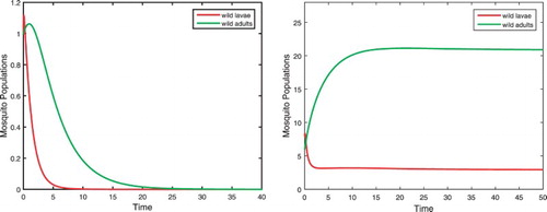
, there exists no positive equilibrium. All solutions go to the origin as shown in the left figure in Figure . For
, there exist two positive equilibria
and
. Equilibrium
is an unstable saddle and
is a stable node. Solutions approach either the origin or
depending on their initial values. We only show a solution approaching
in the right figure in Figure .
Figure 1. Parameters are given in Equation (Equation24(24)
(24) ). For
, there exists no positive equilibrium. Solutions approach the origin as shown in the left figure. For
, there exist two positive equilibria
and
. Solutions approach either the origin or
depending on their initial values. A solution approaching
is shown in the right figure. Here only the curves for wild larvae and adults are presented.
5. Proportional releases
To have a more economically effective strategy for releases of sterile mosquitoes in an area where the population size of wild mosquitoes is relatively small, instead of releasing sterile mosquitoes constantly, we may, by keeping close surveillance of the wild mosquitoes, let the number of releases be proportional to the population size of the wild mosquitos such that [Citation9, Citation18]. In such a case, there possibly exists difficulty for mosquitoes to find mates when the wild mosquito population size is relatively small. Similarly as in Section 2.2, we then assume Allee effects and that the interactive dynamics between the wild and sterile mosquitoes, based on Equation (Equation17
(17)
(17) ), are governed by the following system:
(26)
(26)
The origin is an equilibrium and is always locally asymptotically stable. We then explore the existence of positive equilibria as follows.
At a positive equilibrium of system (Equation26(26)
(26) ), we have
Then it follows from
that the corresponding function for the existence of positive equilibria has the form
where
(27)
(27) with
(28)
(28) Here the threshold value for the releases,
, is defined as
(29)
(29) and
(30)
(30) System (Equation26
(26)
(26) ) clearly has no positive equilibrium if
for any
, or
and
.
Suppose and
. We define
(31)
(31) Then system (Equation26
(26)
(26) ) has no, one, or two positive equilibria provided
,
, or
, respectively.
Similarly as in Section 4, since depends on b, we can determine a threshold value of b for the existence of positive equilibria of system (Equation26
(26)
(26) ) as follows.
Let function be defined as
where
(32)
(32) Then since
and
, i=1,2,3, it follows from
that
is an increasing function of b, which implies that
is monotone increasing as b increases. Therefore, there exists a threshold value
such that as
,
, or
,
,
,
, and hence system (Equation26
(26)
(26) ) has no, one, or two positive equilibria, respectively.
We next study the stability of the positive equilibria. The Jacobian matrix of system (Equation26(26)
(26) ) has the form
The characteristic equation of the linearized system of (Equation26
(26)
(26) ) at an equilibrium then is given by
where
(33)
(33)
Notice that the J component of a positive equilibrium satisfies Equation (Equation27(27)
(27) ). Similarly as in Section 2.2, if there are two positive equilibria, denoted by
and
, where
and
is given in Equation (Equation32
(32)
(32) ), then we have
and
, and hence
and
. By direct calculation, we have
(Details are given in Appendix 1). Thus
and
, and since
, we have
which implies that
is unstable. Furthermore, at
, direct but tedious calculation shows that if
, then
. (Details are given in Appendix 2.) Since
, positive equilibrium
is locally asymptotically stable. In summary, we have the following theorem.
Theorem 5.1.
The trivial equilibrium for system (Equation26
(26)
(26) ) is always locally asymptotically stable. The existence results for positive equilibria of system (Equation26
(26)
(26) ) are summarized in the following table.
Table
The dynamics of system (Equation26(26)
(26) ) have been determined in Theorem 5.1 for
. However, the model dynamics can be complex if
. While
is always an unstable saddle,
can be locally asymptotically stable or unstable. It can be a node or a spiral. We show the dynamical complexity of system (Equation26
(26)
(26) ) in Example 2.
Example 2.
Let parameters be given by
(34)
(34) Note that
. It follows from Equations (Equation29
(29)
(29) ) and (Equation30
(30)
(30) ) that
and then
.
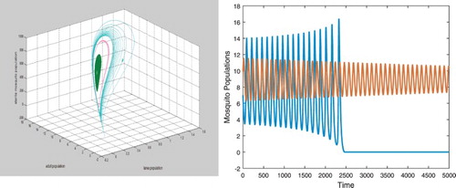
For ,
. There exist two positive equilibria
and
. Equilibrium
is an unstable saddle and
is a stable spiral. There exists an unstable closed orbit as shown in the left figure in Figure . Solutions initially started near
spiral towards
and solutions initially started away from the closed orbit approach the origin as shown in the right figure in Figure .
Figure 2. Parameters are given in Equation (Equation34(34)
(34) ). With b=12.57, there exist positive equilibrium
which is an unstable saddle and positive equilibrium
which is a stable spiral. There exists a unstable closed orbit as shown in the left figure. Solutions initially started near
spiral towards
and solutions initially started away from the closed orbit approach the origin as both shown in the right figure. Here only the curves for the wild adults are presented. Notice that the speed of the convergence to
is slow.
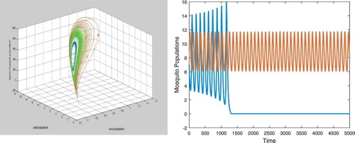
With the same parameters but b=12.5724 which is still less than , we again have two positive equilibria
and
. Equilibrium
is an unstable saddle but
becomes an unstable spiral. There exists a bistable closed orbit as shown in the left figure in Figure . Solutions initially started near
spiral towards the closed orbit and solutions initially started away from the closed orbit approach the origin as shown in the right figure in Figure .
Figure 3. With b=12.57, there are two positive equilibria which is an unstable saddle and
which is an stable spiral. There exists a unstable closed orbit as shown in the left figure. Sustained oscillations occur. Solutions initially started near
spiral towards the bistable closed orbit and solutions initially started away from the closed orbit still approach the origin as both shown in the right figure. Here also only the curves for the wild adults are presented.
6. Proportional releases with saturation
The strategy of proportional releases presented in Section 5, compared to the constant releases, may have an advantage when the size of the wild mosquito population is small since the size of releases is then also small. However, when the wild mosquito population size is large, the release size should presumably also be large, which may exceed our affordability. As in [Citation9, Citation18], we consider a new strategy in which the number of sterile mosquito releases is proportional to the wild mosquito population size when it is small, but is saturated and approaches a constant when the wild mosquito population size increases. Thus, we let the number of the releases be of Holling-II type with the form . Then the interactive system becomes
(35)
(35)
The origin is a trivial equilibrium and is clearly locally asymptotically stable. At a positive equilibrium, we have
where
. Substituting them into the first equation for positive equilibria in Equation (Equation35
(35)
(35) ), we have
Then the equation to determine positive equilibria of Equation (Equation35
(35)
(35) ) is equivalent to
(36)
(36)
Simple calculation yields
and
It follows from
that
Hence
for
, and there exists a unique
, with
, such that
.
Notice that and
,
. Thus
has no, one, or two positive roots, for
, if
,
, or
, respectively.
Similarly as in Sections 4 and 5, we define . Then it follows from
that
is a decreasing function of b and there exists a unique threshold value
such that then if
,
, or
, then
,
, or
, and hence system (Equation35
(35)
(35) ) has no, one, or two positive equilibria, respectively.
We next investigate the stability of the positive equilibria.
At a positive equilibrium, the Jacobian matrix of system (Equation35(35)
(35) ) has the following form:
and hence the characteristic equation is
where
(37)
(37)
Similarly as in Section 5, direct calculation yields
(Details are given in Appendix 3.) If there exist two positive equilibria, denoted by
and
with
, then it follows from
and
that
and
. Hence
which implies the instability of
. At
, direct but tedious calculation shows that if
, then
. (Details are given in Appendix 4.) Since
, positive equilibrium
is locally asymptotically stable. The results are summarized as follows.
Theorem 6.1.
System (Equation35(35)
(35) ) has a trivial equilibrium
which is always locally asymptotically stable. There exists a threshold value
determined by
where
is given in Equation
(Equation36
(36)
(36) ), such that system (Equation35
(35)
(35) ) has no, one, or two positive equilibria if
or
for
respectively. If there exist two positive equilibria
and
with
equilibrium
is an unstable saddle point and
is locally asymptotically provided
.
We note that the stability condition for
is only sufficient and very strong. With most sets of parameters, we have unfortunately not been able to find examples where
is unstable or other dynamical features occur.
7. Concluding remarks
Mosquitoes undergo complete metamorphosis through four distinct stages of development during a lifetime, and the effects of crowding, particularly in the aquatic stages, could be an important factor and thus it is necessary to have the metamorphic stages be included in modelling population dynamics of mosquitoes. Based on the model systems in [Citation9], we introduced the metamorphic stage structure of mosquitoes into dynamical models for interactive wild and sterile mosquitoes to study the impact of the releases of sterile mosquitoes in this paper. We simplified the models by combing the three aquatic metamorphic stages into one group, called larvae as in [Citation15–17], and assumed that the density dependence, due to the intraspecific competition, was only on the larvae. We considered three different strategies similarly as in [Citation9, Citation18] for the releases in model systems (Equation18(18)
(18) ), (Equation26
(26)
(26) ), and (Equation35
(35)
(35) ), respectively. We explored the existence of positive equilibria and studied their stability for all of these model systems. We established threshold release values to determine the existence of positive equilibria for model systems (Equation18
(18)
(18) ) and (Equation26
(26)
(26) ). The threshold value for system (Equation35
(35)
(35) ) was also implicitly obtained. We completely determined the local stability conditions of the equilibria for system (Equation18
(18)
(18) ), and sufficient stability conditions for the positive equilibria for systems (Equation26
(26)
(26) ) and (Equation35
(35)
(35) ) were obtained. The dynamics of system (Equation26
(26)
(26) ) and (Equation35
(35)
(35) ) are complicated. The existence of stable or unstable closed orbits for system (Equation26
(26)
(26) ) is shown in Example 2. While we have obtained sufficient conditions for the stability of the positive equilibria for system (Equation35
(35)
(35) ), the conditions appear too strong and we have been unable to find examples where positive equilibrium
is unstable or where other dynamical phenomena occur when the stability conditions fail.
In principle. the dynamics of the three model systems with different release strategies in this paper are similar to the dynamics of the model systems in [Citation9] where no mosquito metamorphic stages are included. That is, based on threshold release values and under certain conditions, there exist two positive equilibria, one of which is unstable and one of which is locally asymptotically stable for all of the three model systems. System (Equation18(18)
(18) ) has a boundary equilibrium
and systems (Equation26
(26)
(26) ) and (Equation35
(35)
(35) ) have the trivial equilibrium
other than the positive equilibria. Solutions approach either the boundary (or the trivial) equilibrium, or the stable positive equilibrium, depending on their initial values. The comparisons between the three release strategies are also similar to those in [Citation9]. Nevertheless, the analysis is more difficult for the three-dimensional systems in this paper than the two-dimensional systems in [Citation9]. As is illustrated above, the inclusion of the mosquitoes' metamorphic stages and the density dependence in larvae's death rates is necessary from the modelling perspective. On the other hand, we seem to have also learned from this study, as has been well described in many other studies as well, that simplified models may not necessarily lose key features that the more complicated models exhibit. Therefore, it would probably be always a good idea to consider to start with relatively simple models when we work on new real world problems.
Acknowledgments
The authors thank two anonymous reviewers for their careful reading and valuable comments and suggestions.
Disclosure statement
No potential conflict of interest was reported by the authors.
Additional information
Funding
References
- L. Alphey, M. Benedict, R. Bellini, G.G. Clark, D.A. Dame, M.W. Service, and S.L. Dobson, Sterile-insect methods for control of mosquito-borne diseases: An analysis, Vector Borne Zoonotic Dis. 10 (2010), pp. 295–311.
- H.J. Barclay, The sterile insect release method on species with two-stage life cycles, Res. Popul. Ecol. 21 (1980), pp. 165–180.
- H.J. Barclay, Pest population stability under sterile releases, Res. Popul. Ecol. 24 (1982), pp. 405–416.
- H.J. Barclay, Modeling incomplete sterility in a sterile release program: Interactions with other factors, Popul. Ecol. 43 (2001), pp. 197–206.
- H.J. Barclay, Mathematical models for the use of sterile insects, in Sterile Insect Technique. Principles and Practice in Area-Wide Integrated Pest Management, V.A. Dyck, J. Hendrichs, and A.S. Robinson, eds., Springer, Heidelberg, 2005, pp. 147–174.
- H.J. Barclay and M. Mackauer, The sterile insect release method for pest control: A density-dependent model, Environ. Entomol. 9 (1980), pp. 810–817.
- A.C. Bartlett and R.T. Staten, Sterile Insect Release Method and Other Genetic Control Strategies, Radcliffe's IPM World Textbook, 1996. Available at http://ipmworld.umn.edu/chapters/bartlett.htm.
- N. Becker, Mosquitoes and Their Control, Kluwer Academic/Plenum, New York, 2003.
- L. Cai, S. Ai, and J. Li, Dynamics of mosquitoes populations with different strategies for releasing sterile mosquitoes, SIAM J. Appl. Math. 74 (2014), pp. 1786–1809.
- C. Dye, Intraspecific competition amongst larval Aedes aegypti: Food exploitation or chemical interference? Ecol. Entomol. 7 (1982), pp. 39–46.
- K.R. Fister, M.L. McCarthy, S.F. Oppenheimer, and C. Collins, Optimal control of insects through sterile insect release and habitat modification, Math. Biosci. 244 (2013), pp. 201–212.
- J.C. Flores, A mathematical model for wild and sterile species in competition: Immigration, Phys. A 328 (2003), pp. 214–224.
- R.M. Gleiser, J. Urrutia, and D.E. Gorla, Effects of crowding on populations of Aedes albifasciatus larvae under laboratory conditions, Entomologia Experimentalis et Applicata 95 (2000), pp. 135–140.
- J. Li, Differential equations models for interacting wild and transgenic mosquito populations, J. Biol. Dyn. 2 (2008), pp. 241–258.
- J. Li, Simple stage-structured models for wild and transgenic mosquito populations, J. Diff. Eqn. Appl. 17 (2009), pp. 327–347.
- J. Li, Malaria model with stage-structured mosquitoes, Math. Biol. Eng. 8 (2011), pp. 753–768.
- J. Li, Discrete-time models with mosquitoes carrying genetically-modified bacteria, Math. Biosci. 240 (2012), pp. 35–44.
- J. Li and Z. Yuan, Modeling releases of sterile mosquitoes with different strategies, J. Biol. Dyn. 9 (2015), pp. 1–14.
- J. Lu and J. Li, Dynamics of stage-structured discrete mosquito population models, J. Appl. Anal. Comput. 1 (2011), pp. 53–67.
- M. Otero, H.G. Solari, and N. Schweigmann, A stochastic population dynamics model for Aedes aegypti: Formulation and application to a city with temperate climate, Bull. Math. Biol. 68 (2006), pp. 1945–1974.
- C.M. Stone, Transient population dynamics of mosquitoes during sterile male releases: Modelling mating behaviour and perturbations of life history parameters, PlOS ONE 8(9) (2013), pp. 1–13.
- S.M. White, P. Rohani, and S.M. Sait, Modelling pulsed releases for sterile insect techniques: Fitness costs of sterile and transgenic males and the effects on mosquito dynamics, J. Appl. Ecol. 47 (2010), pp. 1329–1339.
- Wikipedia, Sterile Insect Technique, 2014. Available at http://en.wikipedia.org/wiki/Sterile_insect_technique.
- L. Yakob, L. Alphey, and M.B. Bonsall, Aedes aegypti control: The concomitant role of competition, space and transgenic technologies, J. Appl. Ecol. 45 (2008), pp. 1258–1265.
Appendix 1. Calculation of P3
(38)
(38)
Appendix 2. Proof of P1P2 - P3 > 0
It follows from Equation (Equation33(33)
(33) ) that
Write
Then
and we have
It follows from, at a positive equilibrium,
that if we assume
, then
and
(39)
(39) Thus
, if
.
Appendix 3. Calculation of Q3
It follows from, at a positive equilibrium, and
that
. Then
(40)
(40)
Appendix 4. Proof of Q1Q2 - Q3 > 0
It follows from Equation (Equation37(37)
(37) ) that
For convenience, we set
and
. Thus
and we have
If we assume , then
Same as in Equation (EquationA2
(39)
(39) ), we have, if
,
Therefore,
, if
.