Media alert in an SIS epidemic model with logistic growth

ABSTRACT

In general, media coverage would not be implemented unless the number of infected cases reaches some critical number. To reflect this feature, we incorporate the media effect and a critical number of infected cases into the disease transmission rate and consider an susceptible-infected-susceptible epidemic model with logistic growth. Our model analysis shows that early media alert and strong media effects are preferable to decrease the numbers of infected cases at endemic equilibria. Furthermore, we noticed that the model may have up to three endemic equilibria and bi-stability can occur in a threshold interval for the critical number. Note that the interval depends on parameters for the focal disease and the media effect. It is possible to roughly estimate the interval for re-emerging diseases in a given region. Therefore, the result could be useful to health policymakers. Global stability is also obtained when the model admits a unique endemic equilibrium.

KEYWORDS:

• SIS epidemic model
• media alert
• logistic growth
• multiple endemic equilibria
• bi-stability

AMS SUBJECT CLASSIFICATION:

• 34K18
• 34K20
• 92D30

1. Introduction

Media has been utilized as a disease control measure, especially for epidemics associated with emerging and re-emerging infectious diseases [19] such as HIV/AIDS, SARS, H1N1, Ebola virus disease (EVD), Middle East Respiratory Syndrome. During the outbreak of the influenza A (H1N1) in 2009, mass media was extensively used by the Centers for Disease Control and Prevention of United States and WHO to keep the public aware of information related to the pandemic [6]. It is believed that media use contributed to the control of the pandemic. WHO also indicated that media played an important role in controlling the spread of H7N9 in China in 2013 [31]. Media does not only alert the general public on the hazard from the infectious diseases but also informs the public of the requisite preventive measures like wearing protective masks [25], vaccination, voluntary quarantine, avoidance of congregated places, etc. Therefore, the extensive use of media may bring in changes in public behaviour and reduce the frequency and probability of contacts with infected individuals so that the severity of a disease outbreak would be diminished [4, 9, 10, 13, 14, 21, 24].

In order to study the impact of media-like control measures on disease transmission dynamics, several types of media function forms have been proposed to describe reduced disease transmission rates due to media use and compartmental models with these rates have been analysed (e.g. [9, 10, 13–17, 23, 24]). The deduction in the transmission rate was described by the form of $\beta (1-{\mathrm{e}}^{-mI})$ with the parameter m>0 reflecting how strongly media coverage can affect contact infection [9]. With the rate, the analysis of a susceptible–exposed–infected model (SEI) shows that the model may exhibit periodic oscillations for weak media effects while it may have three endemic equilibria for strong media effects [9]. The form of $\beta -{\beta }_{1}I/(\nu +I)$ was also used as the transmission rate with the deduction ${\beta }_{1}I/(\nu +I)$ due to media use [10, 13, 24]. A threshold dynamics was obtained for an SIS epidemic model. It is also shown that media coverage can lower infection and delay the arrival of the infection peak [10, 13]. However, the study of a susceptible–vaccinated–infected–recovered epidemic model with a vaccinated class indicates that media effects could be complicated and simplified understandings may even make the disease worse due to possible public panic [24]. The third function type with psychological/media effects is of the form $\beta /(1+\alpha I^2)$, identified by Collinson and Heffernan (see [8, 33] and the references therein). Using a simple susceptible-exposed-infected-recovered model, Collinson and Heffernan [8] found that important measurements of an epidemic outbreak (such as peak magnitude of infection, peak time of infection peak and end of the outbreak) depend on the chosen media function. Their sensitivity analysis also showed such dependence for the sensitivities of model parameters. This makes it difficult to identify effective disease control strategy and calls for more study on the effects of mass media on disease transmission dynamics.

Theoretical studies usually assume that media coverage affects disease transmission during the whole time period of the disease spread (e.g. [9, 10, 14, 24]). In the reality, media coverage generally does not occur in the beginning stage of a disease spread. For instance, the early suspected cases of EVD died in December 2013 while the first notification by WHO on the outbreak [32] was not issued until 21 March 2014. In general, media delivers alerts and timely reports infected cases only when certain number of infected cases is reached [28, 34, 38]. To include such feature of media/psychological effect, Xiao et al. [34] introduced a critical number of infected cases $I_c$ and proposed a piecewise and discontinuous control function [7, 26] for disease control strategy (sliding mode control). Wang and Xiao [28] further constructed a Filippov SIR epidemic model to describe media effects using the following transmission rate (1) $\beta \left(I\right)=\left\{\begin{array}{ll}\beta ,& I<I_c,\\ \beta \exp (-\alpha I),& I>I_c.\end{array}\right.$(1) Their analysis shows that the model system can stabilize at either one of the equilibria for the resulted subsystems or the new endemic state induced by the on-off media effect, depending on the critical level $I_c$. They also demonstrated that proper combinations of critical levels and control intensities can lead to the desired case number. The transmission rate (1(1) $\beta \left(I\right)=\left\{\begin{array}{ll}\beta ,& I<I_c,\\ \beta \exp (-\alpha I),& I>I_c.\end{array}\right.$(1) ) was then generalized in a time-dependent way to study an influenza outbreak in Shannxi, China [35].

It was demonstrated that compartmental models can exhibit distinct dynamics, depending on the chosen incidence rate (e.g. [20, 33]). To explore the media effect on disease transmission dynamics we here propose a new transmission rate. Following the idea of the critical number of infected cases $I_c$, we consider the following non-smooth but continuous transmission rate: (2) $\beta \left(I\right)=\left\{\begin{array}{ll}\beta ,& 0\le I\le I_c,\\ \beta {\left(\frac{I_c}{I}\right)}^p,& I>I_c,\end{array}\right.$(2) where $p\ge 0$ represents the intensity of the media effect on contact infection. If p=0, $\beta \left(I\right)$ is equal to the background transmission rate β, implying that media coverage does not occur. With this rate, we shall consider an SIS endemic model.

Classical compartmental models with media effects assume either a constant size of the total population or constant recruitment rate for the susceptible class. The assumption of varying total populations may be more reasonable for a relatively long-lasting disease or for a disease with high mortality rates. In fact, varying total populations were discussed before (e.g. [1, 3, 5, 9, 11, 22, 29, 36]). Here, we assume that the population of a community follows the logistic growth. For the sake of mathematical simplicity, we assume that newborns directly enter into the susceptible class and infected persons do not contribute to births and deaths in the susceptible class. Following works in [2, 9, 28], our SIS model reads (3) $\begin{array}{rl}\frac{\mathrm{d}S}{\mathrm{d}t}& =rS\left(1-\frac{S}{a}\right)-\beta \left(I\right)IS+\gamma I,\\ \frac{\mathrm{d}I}{\mathrm{d}t}& =\beta \left(I\right)IS-(d+ϵ+\gamma )I,\end{array}$(3) where r is the intrinsic growth rate of the susceptible population, a denotes the carrying capacity of the community in the absence of infection, d is natural death rate, γ represents the recovered rate, and ε is the disease-induced death rate. The analysis of model (3(3) $\begin{array}{rl}\frac{\mathrm{d}S}{\mathrm{d}t}& =rS\left(1-\frac{S}{a}\right)-\beta \left(I\right)IS+\gamma I,\\ \frac{\mathrm{d}I}{\mathrm{d}t}& =\beta \left(I\right)IS-(d+ϵ+\gamma )I,\end{array}$(3) ) with the transmission rate (2(2) $\beta \left(I\right)=\left\{\begin{array}{ll}\beta ,& 0\le I\le I_c,\\ \beta {\left(\frac{I_c}{I}\right)}^p,& I>I_c,\end{array}\right.$(2) ) shows that there exists a threshold interval Γ for the critical number $I_c$ in which the model may be stabilized at one of two stable equilibria with different levels of infected cases. This implies that the policymaker may have to choose the critical number $I_c$ according to the focal disease in order to minimize infected cases and also avoid unnecessary public panic. The global stability was also obtained for $I_c$ not in the threshold interval. In the following, the analysis of existence of equilibria is presented in Section 2 while the local and global stabilities are given in Sections 3 and 4, respectively. A discussion section comes to the end of the work.

2. Existence of equilibria

For our convenience, denote $b=:r/a$. Model (3(3) $\begin{array}{rl}\frac{\mathrm{d}S}{\mathrm{d}t}& =rS\left(1-\frac{S}{a}\right)-\beta \left(I\right)IS+\gamma I,\\ \frac{\mathrm{d}I}{\mathrm{d}t}& =\beta \left(I\right)IS-(d+ϵ+\gamma )I,\end{array}$(3) ) with the transmission rate (2(2) $\beta \left(I\right)=\left\{\begin{array}{ll}\beta ,& 0\le I\le I_c,\\ \beta {\left(\frac{I_c}{I}\right)}^p,& I>I_c,\end{array}\right.$(2) ) can be decomposed into two sub-systems (4) $\begin{array}{rl}\frac{\mathrm{d}S}{\mathrm{d}t}& =bS(a-S)-\beta IS+\gamma I,\\ \frac{\mathrm{d}I}{\mathrm{d}t}& =\beta IS-(d+ϵ+\gamma )I,\end{array}0\le I\le I_c,$(4) and (5) $\begin{array}{rl}\frac{\mathrm{d}S}{\mathrm{d}t}& =bS(a-S)-\beta {\left(\frac{I_c}{I}\right)}^{p}IS+\gamma I,\\ \frac{\mathrm{d}I}{\mathrm{d}t}& =\beta {\left(\frac{I_c}{I}\right)}^{p}IS-(d+ϵ+\gamma )I,\end{array}I>I_c.$(5) The origin $O(0,0)$ and the disease-free equilibrium $E_0(a,0)$ always exist. The basic reproductive number can be easily calculated, given by ${\mathfrak{R}}_0=\frac{\beta a}{d+ϵ+\gamma },$ from which one can see that media coverage does not change the basic reproduction number (e.g. [9, 10, 13, 15–17, 23, 24]). To obtain the existence of endemic equilibria, denote $a_0\triangleq \frac{a}{{\mathfrak{R}}_0},a_2\triangleq a_0+\frac{d+ϵ}{a_{0}b}{I}_c,I_{\ast }\triangleq \frac{a_0^{2}b}{d+ϵ}({\mathfrak{R}}_0-1),$ and consider two cases: $0\le I\le I_c$ and $I>I_c$, separately.

In the case of $0\le I\le I_c$, the sub-system (4(4) $\begin{array}{rl}\frac{\mathrm{d}S}{\mathrm{d}t}& =bS(a-S)-\beta IS+\gamma I,\\ \frac{\mathrm{d}I}{\mathrm{d}t}& =\beta IS-(d+ϵ+\gamma )I,\end{array}0\le I\le I_c,$(4) ) has a unique positive equilibrium $E_{\ast }(S_{\ast },I_{\ast })$ if and only if $0<I_{\ast }\le I_c$, that is, $a_0<a\le a_2$, where $S_{\ast }=a_0$.

In the case of $I>I_c$, the I component of a positive equilibrium for the sub-system (5(5) $\begin{array}{rl}\frac{\mathrm{d}S}{\mathrm{d}t}& =bS(a-S)-\beta {\left(\frac{I_c}{I}\right)}^{p}IS+\gamma I,\\ \frac{\mathrm{d}I}{\mathrm{d}t}& =\beta {\left(\frac{I_c}{I}\right)}^{p}IS-(d+ϵ+\gamma )I,\end{array}I>I_c.$(5) ) satisfies the following equation (6) $f\left(I\right)={\left(\frac{a_0}{I_c^p}\right)}^{2}b{I}^{2p-1}-\frac{a_0}{I_c^p}ab{I}^{p-1}+(d+ϵ)=0.$(6) From $(a_0/I_c^p{)}^{2}b{I}^{2p-1}-(a_0/I_c^p)ab{I}^{p-1}=-(d+ϵ)<0$, positive solutions to Equation (6(6) $f\left(I\right)={\left(\frac{a_0}{I_c^p}\right)}^{2}b{I}^{2p-1}-\frac{a_0}{I_c^p}ab{I}^{p-1}+(d+ϵ)=0.$(6) ) satisfy (7) $I<{\mathfrak{R}}_0^{1/p}{I}_c\triangleq I_n.$(7) That is, the positive solutions of Equation (6(6) $f\left(I\right)={\left(\frac{a_0}{I_c^p}\right)}^{2}b{I}^{2p-1}-\frac{a_0}{I_c^p}ab{I}^{p-1}+(d+ϵ)=0.$(6) ) must be in the interval $(I_c,I_n)$. Also, $f\left(I_n^{-}\right)=d+ϵ>0$. Therefore, we must have $a>a_0$ due to $I_n>I_c$. Next, we discuss the existence of positive solutions to Equation (6(6) $f\left(I\right)={\left(\frac{a_0}{I_c^p}\right)}^{2}b{I}^{2p-1}-\frac{a_0}{I_c^p}ab{I}^{p-1}+(d+ϵ)=0.$(6) ) in $(I_c,I_n)$ in two cases, $0<p\le 1$ and p>1.

Case I. $0<p\le 1$. In this case, $f\left(I\right)$ is strictly increasing. In fact, the derivative of $f\left(I\right)$ is given by (8) $f^{\prime }\left(I\right)=\frac{a_0}{I_c^p}b{I}^{p-2}\left[\frac{a_0}{I_c^p}(2p-1)I^p-a(p-1)\right],\text{for}I\in (I_c,I_n),$(8) and we can show that $f^{\prime }\left(I\right)>0$ for $0<p\le 1$. If $\frac{1}{2}\le p\le 1$, one clearly derives $f^{\prime }\left(I\right)>0$. If $0<p<\frac{1}{2}$, we can calculate the zero point of $f^{\prime }\left(I\right)$ as (9) $I_{\mathbf{\text{e}}}\triangleq {\left(\frac{p-1}{2p-1}{\mathfrak{R}}_0\right)}^{1/p}{I}_c>0.$(9) which, obviously, $I_{\mathbf{\text{e}}}$ is the unique maximum point of $f\left(I\right)$. Since (10) $I_{\mathbf{\text{e}}}^p-I_n^p=\frac{p}{1-2p}{\mathfrak{R}}_0{I}_c^p,$(10) we have $I_n<I_{\mathbf{\text{e}}}$ for $0<p<\frac{1}{2}$, and hence $f^{\prime }\left(I\right)>0$ on $(I_c,I_n)$. To sum up, we always have $f^{\prime }\left(I\right)>0$ if $0<p\le 1$. Meanwhile, note that (11) $f\left(I_c\right)=\frac{a_{0}b(a_2-a)}{I_c}$(11) may be positive, negative or zero. If $f\left(I_c\right)\ge 0$, which is equivalent to $a\le a_2$, then Equation (6(6) $f\left(I\right)={\left(\frac{a_0}{I_c^p}\right)}^{2}b{I}^{2p-1}-\frac{a_0}{I_c^p}ab{I}^{p-1}+(d+ϵ)=0.$(6) ) has no positive real root in $(I_c,I_n)$. If $f\left(I_c\right)<0$, which is equivalent to $a>a_2$, then Equation (6(6) $f\left(I\right)={\left(\frac{a_0}{I_c^p}\right)}^{2}b{I}^{2p-1}-\frac{a_0}{I_c^p}ab{I}^{p-1}+(d+ϵ)=0.$(6) ) admits a unique positive root, denoted by $I_1$, satisfying $I_c<I_1<I_n$. That is, in the case of $0<p\le 1$, the sub-system (5(5) $\begin{array}{rl}\frac{\mathrm{d}S}{\mathrm{d}t}& =bS(a-S)-\beta {\left(\frac{I_c}{I}\right)}^{p}IS+\gamma I,\\ \frac{\mathrm{d}I}{\mathrm{d}t}& =\beta {\left(\frac{I_c}{I}\right)}^{p}IS-(d+ϵ+\gamma )I,\end{array}I>I_c.$(5) ) has a unique positive equilibrium, denoted by $E_1(S_1,I_1)$, if and only if $a>a_2$, where $S_1=a_0(I_1/I_c{)}^p$ and $I_1\in (I_c,I_n)$.

The following lemma is needed to discuss the case of p>1.

Lemma 2.1:

Let $p>1,$ then $a_1<a_2$ always holds, where $a_1\triangleq {\left[\frac{(2p-1{)}^{2p-1}}{p^p(p-1{)}^{p-1}}\frac{(d+ϵ{)}^p{I}_c^p}{a_0{b}^p}\right]}^{1/(2p-1)}.$

Proof:

Consider the concave function $\mathcal{H}\left(x\right)=\ln x,x>0$. Assign $\begin{array}{rl}{x}_1& =\frac{2p-1}{p-1}{a}_0,x_2=\frac{2p-1}{p}\frac{d+ϵ}{a_{0}b}{I}_c,\\ {\lambda }_1& =\frac{p-1}{2p-1},{\lambda }_2=\frac{p}{2p-1}.\end{array}$ Note that ${\lambda }_1+{\lambda }_2=1$, and $\mathcal{H}\left(x\right)$ is a strictly concave function. This implies that $\mathcal{H}({\lambda }_1{x}_1+{\lambda }_2{x}_2)>{\lambda }_1\mathcal{H}\left(x_1\right)+{\lambda }_2\mathcal{H}\left(x_2\right)$, and we have $\begin{array}{rl}\ln \left(a_0+\frac{d+ϵ}{a_{0}b}{I}_c\right)& =\ln \left(\frac{p-1}{2p-1}\frac{2p-1}{p-1}{a}_0+\frac{p}{2p-1}\frac{2p-1}{p}\frac{d+ϵ}{a_{0}b}{I}_c\right)\\ & >\frac{p-1}{2p-1}\ln \frac{2p-1}{p-1}{a}_0+\frac{p}{2p-1}\ln \frac{2p-1}{p}\frac{d+ϵ}{a_{0}b}{I}_c\\ & =\ln {\left[\frac{2p-1}{p-1}{a}_0\right]}^{(p-1)/(2p-1)}\cdot {\left[\frac{2p-1}{p}\frac{d+ϵ}{a_{0}b}{I}_c\right]}^{p/(2p-1)}\\ & =\ln {\left[\frac{(2p-1{)}^{2p-1}}{p^p(p-1{)}^{p-1}}\frac{(d+ϵ{)}^p{I}_c^p}{a_0{b}^p}\right]}^{1/(2p-1)}.\end{array}$ The monotonicity of $\mathcal{H}\left(x\right)$ leads to $a_1<a_2$. The proof is completed.

Case II. p>1. By Lemma 2.1, $a_1<a_2$ holds. It follow from the formula (10(10) $I_{\mathbf{\text{e}}}^p-I_n^p=\frac{p}{1-2p}{\mathfrak{R}}_0{I}_c^p,$(10) ) that $I_{\mathbf{\text{e}}}<I_n$. Note that the derivative $f^{\prime }\left(I\right)$ given by Equation (8(8) $f^{\prime }\left(I\right)=\frac{a_0}{I_c^p}b{I}^{p-2}\left[\frac{a_0}{I_c^p}(2p-1)I^p-a(p-1)\right],\text{for}I\in (I_c,I_n),$(8) ) is positive. $I_{\mathbf{\text{e}}}$ is the unique minimum point of $f\left(I\right)$. Clearly, $f\left(0^{+}\right)=f\left(I_n^{-}\right)=d+ϵ$. Next, we want to compare the sizes of $I_c$ and $I_{\mathbf{\text{e}}}$ and determine the signs of $f\left(I_c\right)$ and $f\left(I_{\mathbf{\text{e}}}\right)$. The following six cases are considered. Let us denote $I_c^0\triangleq \frac{p}{p-1}\frac{a_0^{2}b}{d+ϵ}.$

Case 1. $I_c\ge I_c^0$ and $a\ge a_2$. It follows from $I_c\ge I_c^0$ that $a_2\ge a_0+\frac{d+ϵ}{a_{0}b}{I}_c^0\ge a_0+\frac{d+ϵ}{a_{0}b}\cdot \frac{p}{p-1}\frac{a_0^{2}b}{d+ϵ}=\frac{2p-1}{p-1}{a}_0.$ Since $a\ge a_2>a_1$, we have $f\left(I_c\right)\le 0$, and $a\ge \left((2p-1)/(p-1)\right)a_0$. Furthermore, from Equation (9(9) $I_{\mathbf{\text{e}}}\triangleq {\left(\frac{p-1}{2p-1}{\mathfrak{R}}_0\right)}^{1/p}{I}_c>0.$(9) ) one can get $I_c\le I_{\mathbf{\text{e}}}$. Thus $f\left(I_{\mathbf{\text{e}}}\right)\le f\left(I_c\right)\le 0$. Direct calculation shows that $a>a_1\iff f\left(I_{\mathbf{\text{e}}}\right)<0$ holds. If $f\left(I_c\right)=0$, we have $I_c<I_{\mathbf{\text{e}}}$. Thus, Equation (6(6) $f\left(I\right)={\left(\frac{a_0}{I_c^p}\right)}^{2}b{I}^{2p-1}-\frac{a_0}{I_c^p}ab{I}^{p-1}+(d+ϵ)=0.$(6) ) has a unique positive root $I_1$, satisfying $I_{\mathbf{\text{e}}}<I_1<I_n$. If $f\left(I_c\right)<0$, the conclusion is still true. Accordingly, the sub-system (5(5) $\begin{array}{rl}\frac{\mathrm{d}S}{\mathrm{d}t}& =bS(a-S)-\beta {\left(\frac{I_c}{I}\right)}^{p}IS+\gamma I,\\ \frac{\mathrm{d}I}{\mathrm{d}t}& =\beta {\left(\frac{I_c}{I}\right)}^{p}IS-(d+ϵ+\gamma )I,\end{array}I>I_c.$(5) ) has a unique positive equilibrium $E_1(S_1,I_1)$.

Case 2. $I_c\ge I_c^0$ and $a_1<a<a_2$. It follows from $I_c\ge I_c^0$ that $\begin{array}{rl}{a}_1& \ge {\left[\frac{(2p-1{)}^{2p-1}}{p^p(p-1{)}^{p-1}}\frac{(d+ϵ{)}^p}{a_0{b}^p}(I_c^0{)}^p\right]}^{1/(2p-1)}\\ & ={\left[\frac{(2p-1{)}^{2p-1}}{p^p(p-1{)}^{p-1}}\frac{(d+ϵ{)}^p}{a_0{b}^p}{\left(\frac{p}{p-1}\frac{a_0^{2}b}{d+ϵ}\right)}^p\right]}^{1/(2p-1)}=\frac{2p-1}{p-1}{a}_0,\end{array}$ that is, $a>\left((2p-1)/(p-1)\right)a_0$. Thus, we have $I_c<I_{\mathbf{\text{e}}}$ from Equation (9(9) $I_{\mathbf{\text{e}}}\triangleq {\left(\frac{p-1}{2p-1}{\mathfrak{R}}_0\right)}^{1/p}{I}_c>0.$(9) ) and $f\left(I_c\right)>0$ because of $a<a_2$. Moreover, one can show that $a>a_1\iff f\left(I_{\mathbf{\text{e}}}\right)<0$. Therefore, when $a_1<a<a_2$, Equation (6(6) $f\left(I\right)={\left(\frac{a_0}{I_c^p}\right)}^{2}b{I}^{2p-1}-\frac{a_0}{I_c^p}ab{I}^{p-1}+(d+ϵ)=0.$(6) ) has two different positive roots in $(I_c,I_n)$, denoted by $I_2$, $I_3$, where $I_2\in (I_c,I_{\mathbf{\text{e}}})$, $I_3\in (I_{\mathbf{\text{e}}},I_n)$. That is, the sub-system (5(5) $\begin{array}{rl}\frac{\mathrm{d}S}{\mathrm{d}t}& =bS(a-S)-\beta {\left(\frac{I_c}{I}\right)}^{p}IS+\gamma I,\\ \frac{\mathrm{d}I}{\mathrm{d}t}& =\beta {\left(\frac{I_c}{I}\right)}^{p}IS-(d+ϵ+\gamma )I,\end{array}I>I_c.$(5) ) admits two different positive equilibria $E_i(S_i,I_i)$, where $S_i=a_0(I_i/I_c{)}^p$, i=2,3.

Case 3. $I_c\ge I_c^0$ and $a=a_1$. Similar to the argument in Case 2, it follows that $\left((2p-1)/(p-1)\right)a_0\le a<a_2$, and hence we have $I_c\le I_{\mathbf{\text{e}}}$ and $f\left(I_c\right)>0$. Note that the equivalent relationship $a=a_1\iff f\left(I_{\mathbf{\text{e}}}\right)=0$. We must have $I_c<I_{\mathbf{\text{e}}}$. This suggests that Equation (6(6) $f\left(I\right)={\left(\frac{a_0}{I_c^p}\right)}^{2}b{I}^{2p-1}-\frac{a_0}{I_c^p}ab{I}^{p-1}+(d+ϵ)=0.$(6) ) only has one positive solution $I_{\mathbf{\text{e}}}\in (I_c,I_n)$. Accordingly, for the sub-system (5(5) $\begin{array}{rl}\frac{\mathrm{d}S}{\mathrm{d}t}& =bS(a-S)-\beta {\left(\frac{I_c}{I}\right)}^{p}IS+\gamma I,\\ \frac{\mathrm{d}I}{\mathrm{d}t}& =\beta {\left(\frac{I_c}{I}\right)}^{p}IS-(d+ϵ+\gamma )I,\end{array}I>I_c.$(5) ), there exists exactly one positive equilibrium $E_{\mathbf{\text{e}}}(S_{\mathbf{\text{e}}},I_{\mathbf{\text{e}}})$, where $S_{\mathbf{\text{e}}}=a_0(I_{\mathbf{\text{e}}}/I_c{)}^p$.

Case 4. $I_c\ge I_c^0$ and $a_0<a<a_1$. Recall that $a<a_1\iff f\left(I_{\mathbf{\text{e}}}\right)>0$ and $I_{\mathbf{\text{e}}}$ is the unique minimum point of $f\left(I\right)$ in $(I_c,I_n)$. One immediately deduces that Equation (6(6) $f\left(I\right)={\left(\frac{a_0}{I_c^p}\right)}^{2}b{I}^{2p-1}-\frac{a_0}{I_c^p}ab{I}^{p-1}+(d+ϵ)=0.$(6) ) has no positive root in $(I_c,I_n)$ no matter $I_c\le I_{\mathbf{\text{e}}}$ or $I_c>I_{\mathbf{\text{e}}}$. Hence, the sub-system (5(5) $\begin{array}{rl}\frac{\mathrm{d}S}{\mathrm{d}t}& =bS(a-S)-\beta {\left(\frac{I_c}{I}\right)}^{p}IS+\gamma I,\\ \frac{\mathrm{d}I}{\mathrm{d}t}& =\beta {\left(\frac{I_c}{I}\right)}^{p}IS-(d+ϵ+\gamma )I,\end{array}I>I_c.$(5) ) has no positive equilibrium.

Case 5. $I_c<I_c^0$ and $a>a_2$. From $a>a_2>a_1$, one deduces that $f\left(I_c\right)<0$ and $f\left(I_{\mathbf{\text{e}}}\right)<0$. Hence, Equation (6(6) $f\left(I\right)={\left(\frac{a_0}{I_c^p}\right)}^{2}b{I}^{2p-1}-\frac{a_0}{I_c^p}ab{I}^{p-1}+(d+ϵ)=0.$(6) ) only has one positive solution $I_1\in (I_c,I_n)$ no matter $I_c\le I_{\mathbf{\text{e}}}$ or $I_c>I_{\mathbf{\text{e}}}$, where $I_{\mathbf{\text{e}}}<I_1<I_n$. That is, the sub-system (5(5) $\begin{array}{rl}\frac{\mathrm{d}S}{\mathrm{d}t}& =bS(a-S)-\beta {\left(\frac{I_c}{I}\right)}^{p}IS+\gamma I,\\ \frac{\mathrm{d}I}{\mathrm{d}t}& =\beta {\left(\frac{I_c}{I}\right)}^{p}IS-(d+ϵ+\gamma )I,\end{array}I>I_c.$(5) ) has only one positive equilibrium $E_1(S_1,I_1)$.

Case 6. $I_c<I_c^0$ and $a_0<a\le a_2$. Clearly, one can have $a_2<\left((2p-1)/(p-1)\right)a_0$ from $I_c<I_c^0$ and $a\le a_2<\left((2p-1)/(p-1)\right)a_0$. Hence, $I_{\mathbf{\text{e}}}<I_c$. Notice that $f\left(I\right)$ is an increasing function on the interval $(I_c,I_n)$, and $f\left(I_c\right)\ge 0$. Equation (6(6) $f\left(I\right)={\left(\frac{a_0}{I_c^p}\right)}^{2}b{I}^{2p-1}-\frac{a_0}{I_c^p}ab{I}^{p-1}+(d+ϵ)=0.$(6) ) has no positive root in the interval $(I_c,I_n)$. Namely, the sub-system (5(5) $\begin{array}{rl}\frac{\mathrm{d}S}{\mathrm{d}t}& =bS(a-S)-\beta {\left(\frac{I_c}{I}\right)}^{p}IS+\gamma I,\\ \frac{\mathrm{d}I}{\mathrm{d}t}& =\beta {\left(\frac{I_c}{I}\right)}^{p}IS-(d+ϵ+\gamma )I,\end{array}I>I_c.$(5) ) has no positive equilibrium.

Now, one summarizes the existence of the equilibria of model (3(3) $\begin{array}{rl}\frac{\mathrm{d}S}{\mathrm{d}t}& =rS\left(1-\frac{S}{a}\right)-\beta \left(I\right)IS+\gamma I,\\ \frac{\mathrm{d}I}{\mathrm{d}t}& =\beta \left(I\right)IS-(d+ϵ+\gamma )I,\end{array}$(3) ) as follows:

Theorem 2.2:

Model (3(3) $\begin{array}{rl}\frac{\mathrm{d}S}{\mathrm{d}t}& =rS\left(1-\frac{S}{a}\right)-\beta \left(I\right)IS+\gamma I,\\ \frac{\mathrm{d}I}{\mathrm{d}t}& =\beta \left(I\right)IS-(d+ϵ+\gamma )I,\end{array}$(3) ) always admits an equilibrium $O(0,0)$ and a disease-free equilibrium $E_0(a,0)$. If $a\le a_0$ $($i.e. ${\mathfrak{R}}_0\le 1),$ then model (3(3) $\begin{array}{rl}\frac{\mathrm{d}S}{\mathrm{d}t}& =rS\left(1-\frac{S}{a}\right)-\beta \left(I\right)IS+\gamma I,\\ \frac{\mathrm{d}I}{\mathrm{d}t}& =\beta \left(I\right)IS-(d+ϵ+\gamma )I,\end{array}$(3) ) has no endemic equilibrium. If $a>a_0$ $($i.e. ${\mathfrak{R}}_0>1),$ we have the following conclusions.

1. Assume that $0<p\le 1$.

   1. If $a_0<a\le a_2,$ then $E_{\ast }$ is a unique endemic equilibrium;

   2. If $a>a_2,$ then $E_1$ is a unique endemic equilibrium.

2. Assume that p>1 and $I_c\ge I_c^0$.

   1. If $a_0<a<a_1,$ $E_{\ast }$ is a unique endemic equilibrium;

   2. If $a=a_1,$ there are two endemic equilibrium, $E_{\ast }$ and $E_{\mathbf{\text{e}}};$

   3. If $a_1<a<a_2,$ there exist three endemic equilibria, $E_{\ast },$ $E_2$ and $E_3;$

   4. If $a=a_2,$ both $E_{\ast }$ and $E_1$ exist;

   5. If $a>a_2,$ $E_1$ is a unique endemic equilibrium.

3. Assume that p>1 and $I_c<I_c^0$.

   1. If $a_0<a\le a_2,$ $E_{\ast }$ is a unique endemic equilibrium;

   2. If $a>a_2,$ $E_1$ is a unique endemic equilibrium.

Remark 1:

From (ii) of (1), (v) of (2) and (iii) of (3) in Theorem 2.2 one can deduce that $E_1$ is a unique endemic equilibrium if $a>a_2$.

By Theorem 2.2, if $0<p\le 1$, model (3) only has one endemic equilibrium, either $E_{\ast }$ (in the case of $a_0<a\le a_2$), or $E_1$ (in the case of $a>a_2$). The existence of positive equilibria for the model in the case of p>1 is illustrated in Figure 1. Here, we define the following different curves and regions for parameters a and $I_c$ as follows: $L_0=\left\{\right(a,I_c)\mid a=a_0\}$, $L_1=\left\{\right(a,I_c)\mid a=a_1\text{and}{I}_c\ge I_c^0\}$, $L_2=\left\{\right(a,I_c)\mid a=a_2\text{and}{I}_c\ge I_c^0\}$, $Q_1=\left\{\right(a,I_c)\mid a>a_2\}$, $Q_2=\left\{\right(a,I_c)\mid a_1<a<a_2\text{and}{I}_c\ge I_c^0\}$, $Q_3=C_U(Q_2\cup L_1\cup L_2)$ (where $U=\left\{\right(a,I_c)\mid a_0<a\le a_2\}$), and $Q_4=\left\{\right(a,I_c)\mid 0<a\le a_1\}$.

Figure 1. The existence of the endemic equilibria of model (3(3) $\begin{array}{rl}\frac{\mathrm{d}S}{\mathrm{d}t}& =rS\left(1-\frac{S}{a}\right)-\beta \left(I\right)IS+\gamma I,\\ \frac{\mathrm{d}I}{\mathrm{d}t}& =\beta \left(I\right)IS-(d+ϵ+\gamma )I,\end{array}$(3) ) in the case of p>1. There are equilibria $E_{\ast }$ and $E_{\mathbf{\text{e}}}$ on the curve $L_1$, $E_{\ast }$ and $E_1$ on $L_2$, three equilibria $E_{\ast }$, $E_2$ and $E_3$ in the region $Q_2$, a unique equilibrium $E_1$ in the region $Q_1$, a unique equilibrium $E_{\ast }$ in the region $Q_3$, and no endemic equilibrium in $Q_4$. See the content for the definitions of these regions.

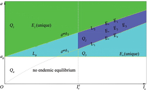
Note that the condition $a_1\le a\le a_2$ with $I_c>I_c^0$ in Theorem 2.2 is equivalent to $I_c^1\le I_c\le I_c^2$, where $I_c^1=max\{I_{\ast },I_c^0\},I_c^2={\left[\frac{p^p(p-1{)}^{p-1}}{(2p-1{)}^{2p-1}}\frac{a^{2p-2}}{{\mathfrak{R}}_0}\right]}^{1/p}\frac{b}{d+ϵ}.$ In the case of ${\mathfrak{R}}_0>1$ and p>1, multiple endemic equilibria exist if the critical number $I_c$ is in the threshold interval (12) $\mathrm{\Gamma }:=[I_c^1,I_c^2].$(12) The existence region in Figure 1 is given by the union of $L_1$, $L_2$ and $Q_2$.

3. Local stability of equilibria

This section focuses on the local stability of equilibria. Corresponding to the equilibria $O(0,0)$, $E_0$ and $E_{\ast }$, the Jacobian matrix of the sub-system (4(4) $\begin{array}{rl}\frac{\mathrm{d}S}{\mathrm{d}t}& =bS(a-S)-\beta IS+\gamma I,\\ \frac{\mathrm{d}I}{\mathrm{d}t}& =\beta IS-(d+ϵ+\gamma )I,\end{array}0\le I\le I_c,$(4) ) reads (13) $J=\left(\begin{array}{cc}ab-2bS-\beta I& -\beta S+\gamma \\ \beta I& \beta S-(d+ϵ+\gamma )\end{array}\right).$(13) At $O(0,0)$ the determinant $det\left(J\right(O\left)\right)=-ab(d+ϵ+\gamma )<0$. Thus $O(0,0)$ is a saddle point. At $E_0(a,0)$ it can be shown that (14) $\begin{array}{rl}det\left(J\right(E_0\left)\right)& =-\beta ab(a-a_0),\\ \mathrm{tr}\left(J\right(E_0\left)\right)& =\beta (a-a_0)-ab.\end{array}$(14) If $a>a_0$, then $det\left(J\right(E_0\left)\right)<0$, which means that $E_0$ is a saddle point. If $a<a_0$, then $det\left(J\right(E_0\left)\right)>0$ and $\mathrm{tr}\left(J\right(E_0\left)\right)<0$. Hence $E_0$ is locally asymptotically stable. Since (15) $[-\mathrm{tr}(J\left(E_0\right)){]}^2-4det(J\left(E_0\right))=[\beta (a-a_0)+ab{]}^2\ge 0,$(15) $E_0$ is a stable node or critical node or degenerate node. If $a=a_0$, it follows from $det\left(J\right(E_0\left)\right)=0$, $\mathrm{tr}\left(J\right(E_0\left)\right)<0$ that $E_0$ is a saddle-node (see Theorem 7.1 in [37] or Theorem 2.11.1 in [18]).

The Jacobian matrix at $E_{\ast }(S_{\ast },I_{\ast })$ can be written as (16) $J\left(E_{\ast }\right)=\left(\begin{array}{cc}-\frac{\gamma b(a-a_0)}{d+ϵ}-a_0& -(d+ϵ)\\ \frac{b(d+ϵ+\gamma )(a-a_0)}{d+ϵ}& 0\end{array}\right).$(16) And hence, (17) $\begin{array}{rl}det\left(J\right(E_{\ast }\left)\right)& =b(d+ϵ+\gamma )(a-a_0),\\ \mathrm{tr}\left(J\right(E_{\ast }\left)\right)& =-\frac{\gamma b(a-a_0)}{d+ϵ}-a_0.\end{array}$(17) Recall that $a>a_0$ holds when $E_{\ast }$ exists. We have $det\left(J\right(E_{\ast }\left)\right)>0$, $\mathrm{tr}\left(J\right(E_{\ast }\left)\right)<0$. Thus, $E_{\ast }$ is asymptotically stable.

In the following, we discuss the stability of the equilibria $E_i$, $i=\mathbf{\text{e}},1,2,3$. The Jacobian matrix of the sub-system (5(5) $\begin{array}{rl}\frac{\mathrm{d}S}{\mathrm{d}t}& =bS(a-S)-\beta {\left(\frac{I_c}{I}\right)}^{p}IS+\gamma I,\\ \frac{\mathrm{d}I}{\mathrm{d}t}& =\beta {\left(\frac{I_c}{I}\right)}^{p}IS-(d+ϵ+\gamma )I,\end{array}I>I_c.$(5) ) at $E_i$ is given by (18) $M=\left(\begin{array}{cc}ab-2a_{0}b{\left(\frac{I_i}{I_c}\right)}^p-\beta I_c^p{I}_i^{1-p}& p(d+ϵ+\gamma )-(d+ϵ)\\ \beta I_c^p{I}_i^{1-p}& -p(d+ϵ+\gamma )\end{array}\right).$(18) By Equation (6(6) $f\left(I\right)={\left(\frac{a_0}{I_c^p}\right)}^{2}b{I}^{2p-1}-\frac{a_0}{I_c^p}ab{I}^{p-1}+(d+ϵ)=0.$(6) ), we have (19) $I_i^{1-p}=\frac{a_0}{I_c^p(d+ϵ)}\left(a-a_0{\left(\frac{I_i}{I_c}\right)}^p\right).$(19) Hence, (20) $\begin{array}{rl}\mathrm{tr}\left(M\right(E_i\left)\right)& =a-2a_0{\left(\frac{I_i}{I_c}\right)}^p-\beta I_c^p{I}_i^{1-p}-p(d+ϵ+\gamma )\\ & =\frac{a_0[\gamma -(d+ϵ\left)\right]}{d+ϵ}{\left(\frac{I_i}{I_c}\right)}^p-\frac{\gamma a+p(d+ϵ+\gamma )(d+ϵ)}{d+ϵ}.\end{array}$(20) If $\gamma \le d+ϵ$, then $\mathrm{tr}\left(M\right(E_i\left)\right)<0$ always holds. If $\gamma >d+ϵ$, from $I_i<I_n={\mathfrak{R}}_0^{1/p}{I}_c$, it follows that (21) $\begin{array}{rl}\mathrm{tr}\left(M\right(E_i\left)\right)& <\frac{a[\gamma -(d+ϵ\left)\right]}{d+ϵ}-\frac{\gamma a+p(d+ϵ+\gamma )(d+ϵ)}{d+ϵ}\\ & =-[a+p(d+ϵ+\gamma \left)\right]\\ & <0.\end{array}$(21) Therefore, we always have $\mathrm{tr}\left(M\right(E_i\left)\right)<0$.

From formula (19(19) $I_i^{1-p}=\frac{a_0}{I_c^p(d+ϵ)}\left(a-a_0{\left(\frac{I_i}{I_c}\right)}^p\right).$(19) ), one can have (22) $\begin{array}{rl}det\left(M\right(E_i\left)\right)& =2a_0(d+ϵ+\gamma ){\left(\frac{I_i}{I_c}\right)}^p-\beta I_c^p(d+ϵ)I_i^{1-p}-pa(d+ϵ+\gamma )\\ & =a_0(d+ϵ+\gamma )\left[(2p-1){\left(\frac{I_i}{I_c}\right)}^p-(p-1){\mathfrak{R}}_0\right].\end{array}$(22) Let us first determine the sign of $det\left(M\right(E_i\left)\right)$ at the equilibrium $E_1$. If $\frac{1}{2}\le p\le 1$, both terms in the bracket of formula (22(22) $\begin{array}{rl}det\left(M\right(E_i\left)\right)& =2a_0(d+ϵ+\gamma ){\left(\frac{I_i}{I_c}\right)}^p-\beta I_c^p(d+ϵ)I_i^{1-p}-pa(d+ϵ+\gamma )\\ & =a_0(d+ϵ+\gamma )\left[(2p-1){\left(\frac{I_i}{I_c}\right)}^p-(p-1){\mathfrak{R}}_0\right].\end{array}$(22) ) are positive and hence $det\left(M\right(E_1\left)\right)>0$. If $0<p<\frac{1}{2}$, from Case I in Section 2 we know $I_1<I_n<I_{\mathbf{\text{e}}}$. Therefore, (23) $det\left(M\right(E_1\left)\right)>a_0(d+ϵ+\gamma )\left[(2p-1){\left(\frac{I_{\mathbf{\text{e}}}}{I_c}\right)}^p-(p-1){\mathfrak{R}}_0\right]=0.$(23)

If p>1, from the discussion of Cases 1 and 5 in Section 2 it follows that $I_1>I_{\mathbf{\text{e}}}$, implying that inequality (23(23) $det\left(M\right(E_1\left)\right)>a_0(d+ϵ+\gamma )\left[(2p-1){\left(\frac{I_{\mathbf{\text{e}}}}{I_c}\right)}^p-(p-1){\mathfrak{R}}_0\right]=0.$(23) ) still holds. In summary, we have $det\left(M\right(E_1\left)\right)>0$ and $\mathrm{tr}\left(M\right(E_1\left)\right)<0$. Therefore, $E_1$ is asymptotically stable. The stability of the equilibria $E_{\mathbf{\text{e}}}$, $E_2$ and $E_3$ can be determined similarly. At $E_{\mathbf{\text{e}}}$, one can have $det\left(M\right(E_{\mathbf{\text{e}}}\left)\right)=0$, implying that $E_{\mathbf{\text{e}}}$ is a degenerate node. At $E_2$, it follows from $I_2<I_{\mathbf{\text{e}}}$ that $det\left(M\right(E_2\left)\right)<0$. Thus, $E_2$ is a saddle point. At $E_3$, we have $det\left(M\right(E_3\left)\right)>0$ (since $I_3>I_{\mathbf{\text{e}}}$). Hence, $E_3$ is stable.

To sum up, one obtains the following result.

Theorem 3.1:

For model (3(3) $\begin{array}{rl}\frac{\mathrm{d}S}{\mathrm{d}t}& =rS\left(1-\frac{S}{a}\right)-\beta \left(I\right)IS+\gamma I,\\ \frac{\mathrm{d}I}{\mathrm{d}t}& =\beta \left(I\right)IS-(d+ϵ+\gamma )I,\end{array}$(3) ), the local stability of the equilibria is stated as follows:

1. The origin $O(0,0)$ is a saddle point;

2. If $a<a_0$ $($i.e. ${\mathfrak{R}}_0<1),$ then the disease-free equilibrium $E_0$ is locally stable. If $a=a_0,$ then $E_0$ is a saddle-node. If $a>a_0$ $($i.e. ${\mathfrak{R}}_0>1),$ then $E_0$ is a saddle point;

3. $E_{\ast },$ $E_1,$ $E_3$ are locally asymptotically stable whenever they exist. $E_2$ is a saddle point, and $E_{\mathbf{\text{e}}}$ is a degenerate node.

To illustrate the existence and stabilities of multiple equilibria for model (3(3) $\begin{array}{rl}\frac{\mathrm{d}S}{\mathrm{d}t}& =rS\left(1-\frac{S}{a}\right)-\beta \left(I\right)IS+\gamma I,\\ \frac{\mathrm{d}I}{\mathrm{d}t}& =\beta \left(I\right)IS-(d+ϵ+\gamma )I,\end{array}$(3) ), we utilize some parameter values estimated from the influenza A (H1N1). Set the recovered rate $\gamma =0.0196$ year⁻¹ [12], the disease-induced death rate $ϵ=2.7397$ year⁻¹ [25], and fix the natural death rate $d=\frac{1}{75}$ year⁻¹, and $b=1.9237\times {10}^{-3}$. The basic reproductive number of influenza A was estimated as 1.5−3.1 [30]. For ease of demonstration, we naively set p=3, $\beta =0.0139$ and a=600, and hence the basic reproductive number ${\mathfrak{R}}_0$ is equal to 3.0. We shall consider two examples. Both examples show the occurrence of bi-stability, in which solutions may converge to one of two stable equilibria, depending on initial conditions.

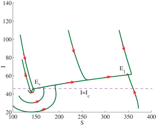
Example 3.1:

Set $I_c=45$. We can calculate $I_c^0=21$ and $a_2=600$. Therefore, $I_c>I_c^0$, and $a=a_2$. In this case (see Theorem 2.2(2)), model (3(3) $\begin{array}{rl}\frac{\mathrm{d}S}{\mathrm{d}t}& =rS\left(1-\frac{S}{a}\right)-\beta \left(I\right)IS+\gamma I,\\ \frac{\mathrm{d}I}{\mathrm{d}t}& =\beta \left(I\right)IS-(d+ϵ+\gamma )I,\end{array}$(3) ) admits two stable endemic equilibria $E_{\ast }$ and $E_1$, that is, bi-stability occurs (see the line $L_2$ in Figure 1). Some solutions to the model are illustrated in Figure 2. Note that $a=a_2$ is equivalent to $I_c=I_{\ast }$. The endemic equilibrium $E_{\ast }$ lies on the horizontal line $I=I_c$.

Figure 2. Phase plot of I verses S showing that two stable endemic equilibria $E_{\ast }$, $E_1$ coexist. Here, we fix $(a,b,\beta ,d,\gamma ,ϵ)=(600,1.9237\times {10}^{-3},0.0139,\frac{1}{75},0.0196,2.7397)$, and set $I_c=45>I_c^0=21$.

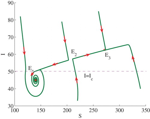
Example 3.2:

Set $I_c=50$. In this case, $I_c>I_c^0=21$, $a_1=597$ and $a_2=651$. The conditions of (iii) of (2) in Theorem 2.2 are satisfied. Hence, model (3(3) $\begin{array}{rl}\frac{\mathrm{d}S}{\mathrm{d}t}& =rS\left(1-\frac{S}{a}\right)-\beta \left(I\right)IS+\gamma I,\\ \frac{\mathrm{d}I}{\mathrm{d}t}& =\beta \left(I\right)IS-(d+ϵ+\gamma )I,\end{array}$(3) ) has three positive equilibria $E_{\ast }$, $E_2$ and $E_3$. Figure 3 illustrates some numerical solutions to the model. The stable manifolds of the saddle $E_2$ split the phase plane into two regions. In the lower region, solutions approach to $E_{\ast }$ while in the upper region solutions approach to $E_3$ (see Figure 3).

Figure 3. Phase plot of I verses S showing that bi-stability occurs for $I_c>I_c^0$ and $a_1<a<a_2$. Here, $E_{\ast }$ and $E_3$ are locally stable while $E_2$ is a saddle point. $I_c=50>I_c^0=21$ and other parameters take the same values as in Figure 2.

4. Global stability analysis

In this section, we study the global stability of model (3(3) $\begin{array}{rl}\frac{\mathrm{d}S}{\mathrm{d}t}& =rS\left(1-\frac{S}{a}\right)-\beta \left(I\right)IS+\gamma I,\\ \frac{\mathrm{d}I}{\mathrm{d}t}& =\beta \left(I\right)IS-(d+ϵ+\gamma )I,\end{array}$(3) ). It can be shown that the state variables of model (3(3) $\begin{array}{rl}\frac{\mathrm{d}S}{\mathrm{d}t}& =rS\left(1-\frac{S}{a}\right)-\beta \left(I\right)IS+\gamma I,\\ \frac{\mathrm{d}I}{\mathrm{d}t}& =\beta \left(I\right)IS-(d+ϵ+\gamma )I,\end{array}$(3) ) remain non-negative for non-negative initial conditions. Consider the biologically feasible region $\mathrm{\Pi }=\left\{(S,I)\in {\mathcal{R}}_{+}^2:N=S+I\le K_0=\frac{(ab+d+ϵ{)}^2}{4b^2(d+\gamma )}+1\right\}.$ Choosing the straight line S+I−Ab=0, similar to the proof of Corollary in [36], we have the following two results.

Lemma 4.1:

The closed set Π is a positively invariant set for model (3(3) $\begin{array}{rl}\frac{\mathrm{d}S}{\mathrm{d}t}& =rS\left(1-\frac{S}{a}\right)-\beta \left(I\right)IS+\gamma I,\\ \frac{\mathrm{d}I}{\mathrm{d}t}& =\beta \left(I\right)IS-(d+ϵ+\gamma )I,\end{array}$(3) ).

Theorem 4.2:

$E_0$ is globally asymptotically stable if $0<a\le a_0$ and unstable if $a>a_0$.

To the best of our knowledge, by precluding the existence of a limit cycle we are able to prove global stability of the unique endemic equilibrium of model (3(3) $\begin{array}{rl}\frac{\mathrm{d}S}{\mathrm{d}t}& =rS\left(1-\frac{S}{a}\right)-\beta \left(I\right)IS+\gamma I,\\ \frac{\mathrm{d}I}{\mathrm{d}t}& =\beta \left(I\right)IS-(d+ϵ+\gamma )I,\end{array}$(3) ).

Theorem 4.3:

There exist no limit cycles for model (3(3) $\begin{array}{rl}\frac{\mathrm{d}S}{\mathrm{d}t}& =rS\left(1-\frac{S}{a}\right)-\beta \left(I\right)IS+\gamma I,\\ \frac{\mathrm{d}I}{\mathrm{d}t}& =\beta \left(I\right)IS-(d+ϵ+\gamma )I,\end{array}$(3) ).

Proof:

The following two steps are considered to achieve our conclusion.

Step 1. We shall prove that there are no limit cycles in the region below the line $I=I_c$ in the feasible region Π and in the region above the line $I=I_c$. Denote these two regions by ${\mathrm{\Pi }}_1$ and ${\mathrm{\Pi }}_2$.

Take the Dulac function $D(S,I)=S^{-1}$. In the case of $0<I\le I_c$, by the transformation (24) $x=S,y=\ln I,$(24) one can transfer sub-system (4(4) $\begin{array}{rl}\frac{\mathrm{d}S}{\mathrm{d}t}& =bS(a-S)-\beta IS+\gamma I,\\ \frac{\mathrm{d}I}{\mathrm{d}t}& =\beta IS-(d+ϵ+\gamma )I,\end{array}0\le I\le I_c,$(4) ) into (25) $\begin{array}{rl}\frac{\mathrm{d}x}{\mathrm{d}t}& =bx(a-x)-(\beta x-\gamma ){\mathrm{e}}^y,\\ \frac{\mathrm{d}y}{\mathrm{d}t}& =\beta x-(d+ϵ+\gamma ).\end{array}$(25) and $D(x,y)=x^{-1}$. Let $N_1$, $N_2$ be the right-hand side functions of (25(25) $\begin{array}{rl}\frac{\mathrm{d}x}{\mathrm{d}t}& =bx(a-x)-(\beta x-\gamma ){\mathrm{e}}^y,\\ \frac{\mathrm{d}y}{\mathrm{d}t}& =\beta x-(d+ϵ+\gamma ).\end{array}$(25) ). Then (26) $\frac{\mathrm{\partial }\left(D{N}_1\right)}{\mathrm{\partial }x}+\frac{\mathrm{\partial }\left(D{N}_2\right)}{\mathrm{\partial }y}=-\frac{\gamma {\mathrm{e}}^y}{x^2}-b<0.$(26) Therefore, there are no limit cycles in the region below the line $I=I_c$.

In the case of $I>I_c$, we can extend subsystem (5(5) $\begin{array}{rl}\frac{\mathrm{d}S}{\mathrm{d}t}& =bS(a-S)-\beta {\left(\frac{I_c}{I}\right)}^{p}IS+\gamma I,\\ \frac{\mathrm{d}I}{\mathrm{d}t}& =\beta {\left(\frac{I_c}{I}\right)}^{p}IS-(d+ϵ+\gamma )I,\end{array}I>I_c.$(5) ) to the case of $I\ge I_c$ because of the continuity of the transmission function $\beta \left(I\right)$. That is, subsystem (5(5) $\begin{array}{rl}\frac{\mathrm{d}S}{\mathrm{d}t}& =bS(a-S)-\beta {\left(\frac{I_c}{I}\right)}^{p}IS+\gamma I,\\ \frac{\mathrm{d}I}{\mathrm{d}t}& =\beta {\left(\frac{I_c}{I}\right)}^{p}IS-(d+ϵ+\gamma )I,\end{array}I>I_c.$(5) ) can be rewritten into (27) $\begin{array}{rl}\frac{\mathrm{d}S}{\mathrm{d}t}& =bS(a-S)-\beta {\left(\frac{I_c}{I}\right)}^{p}IS+\gamma I,\\ \frac{\mathrm{d}I}{\mathrm{d}t}& =\beta {\left(\frac{I_c}{I}\right)}^{p}IS-(d+ϵ+\gamma )I,\end{array}I\ge I_c.$(27) Consider two cases p=1 and $p\ne 1$. If p=1, one can set x=S and y=I. With $N_1$ and $N_2$ being the right sides of system (27(27) $\begin{array}{rl}\frac{\mathrm{d}S}{\mathrm{d}t}& =bS(a-S)-\beta {\left(\frac{I_c}{I}\right)}^{p}IS+\gamma I,\\ \frac{\mathrm{d}I}{\mathrm{d}t}& =\beta {\left(\frac{I_c}{I}\right)}^{p}IS-(d+ϵ+\gamma )I,\end{array}I\ge I_c.$(27) ), direct calculations show that (28) $\frac{\mathrm{\partial }\left(D{N}_1\right)}{\mathrm{\partial }x}+\frac{\mathrm{\partial }\left(D{N}_2\right)}{\mathrm{\partial }y}=-\frac{\gamma y}{x^2}-\frac{d+ϵ+\gamma }{x}-b<0.$(28) If $p\ne 1$, using the transformation (29) $x=S,y=\ln I^{1-p},$(29) one obtains (30) $\begin{array}{rl}\frac{\mathrm{d}x}{\mathrm{d}t}& =bx(a-x)-\beta I_c^{p}x{\mathrm{e}}^y+\gamma {\mathrm{e}}^{y/(1-p)},\\ \frac{\mathrm{d}y}{\mathrm{d}t}& =(1-p)[\beta I_c^{p}x{\mathrm{e}}^{-py/(1-p)}-(d+ϵ+\gamma \left)\right].\end{array}$(30) Therefore, (31) $\frac{\mathrm{\partial }\left(D{N}_1\right)}{\mathrm{\partial }x}+\frac{\mathrm{\partial }\left(D{N}_2\right)}{\mathrm{\partial }y}=-\frac{\gamma }{x^2}{\mathrm{e}}^{y/(1-p)}-p\beta I_c^p{\mathrm{e}}^{-py/(1-p)}-b<0.$(31) Consequently, for all p>0, one can have (32) $\frac{\mathrm{\partial }\left(D{N}_1\right)}{\mathrm{\partial }x}+\frac{\mathrm{\partial }\left(D{N}_2\right)}{\mathrm{\partial }y}<0.$(32) Hence, there is no limit cycle in ${\mathrm{\Pi }}_2$, the region above the line $I=I_c$. We should point out that inequalities (26(26) $\frac{\mathrm{\partial }\left(D{N}_1\right)}{\mathrm{\partial }x}+\frac{\mathrm{\partial }\left(D{N}_2\right)}{\mathrm{\partial }y}=-\frac{\gamma {\mathrm{e}}^y}{x^2}-b<0.$(26) ) and (32(32) $\frac{\mathrm{\partial }\left(D{N}_1\right)}{\mathrm{\partial }x}+\frac{\mathrm{\partial }\left(D{N}_2\right)}{\mathrm{\partial }y}<0.$(32) ) hold for $y\in (-\mathrm{\infty },+\mathrm{\infty })$.

Step 2. We are now ready to show that model (3(3) $\begin{array}{rl}\frac{\mathrm{d}S}{\mathrm{d}t}& =rS\left(1-\frac{S}{a}\right)-\beta \left(I\right)IS+\gamma I,\\ \frac{\mathrm{d}I}{\mathrm{d}t}& =\beta \left(I\right)IS-(d+ϵ+\gamma )I,\end{array}$(3) ) has no limit cycle crossing the line $I=I_c$. The idea is similar to that in [27, 28, 34].

Assume that Γ is a limit cycle across the line $I=I_c$. Let ${\mathrm{\Gamma }}_1$ be the part of the cycle below $I=I_c$ of the cycle Γ, and ${\mathrm{\Gamma }}_2$ be the part above $I=I_c$, with the direction designated in Figure 4. Let both ${\mathrm{\Gamma }}_1$ and ${\mathrm{\Gamma }}_2$ include two intersection points $C_1$, $C_2$ of Γ with the line $I=I_c$. The region enclosed by ${\mathrm{\Gamma }}_1$ and the segment $C_1{C}_2$ is denoted by $G_1$, and the region enclosed by ${\mathrm{\Gamma }}_2$ and the segment $C_1{C}_2$ is denoted by $G_2$.

Figure 4. A limit cycle intersects with the line $I=I_c$ at $C_1$ and $C_2$.

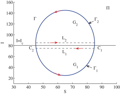
Let us choose two the directed-paths $L_1:\overrightarrow{C_1{C}_2}$ and $L_2:\overrightarrow{C_2{C}_1}$, as shown in Figure 4. It can be seen that (33) $\begin{array}{rl}{\oint }_{{\mathrm{\Gamma }}_1\cup {\mathrm{\Gamma }}_2}D(N_1\mathrm{d}I-N_2\mathrm{d}S)& =\left({\int }_{{\mathrm{\Gamma }}_1}+{\int }_{{\mathrm{\Gamma }}_2}\right)D(N_1\mathrm{d}I-N_2\mathrm{d}S)\\ & =\left({\int }_{{\mathrm{\Gamma }}_1}+{\int }_{{\mathrm{\Gamma }}_2}+{\int }_{L_1}+{\int }_{L_2}-{\int }_{L_1}-{\int }_{L_2}\right)D(N_1\mathrm{d}I-N_2\mathrm{d}S)\\ & =\left({\oint }_{{\mathrm{\Gamma }}_1\cup L_1}+{\oint }_{{\mathrm{\Gamma }}_2\cup L_2}-{\int }_{L_1}-{\int }_{L_2}\right)D(N_1\mathrm{d}I-N_2\mathrm{d}S).\end{array}$(33) Meanwhile, it is easy to obtain that (34) $\left({\int }_{L_1}+{\int }_{L_2}\right)D(N_1\mathrm{d}I-N_2\mathrm{d}S)=0.$(34) Hence, from Green's Theorem it follows that (35) $\begin{array}{rl}{\oint }_{{\mathrm{\Gamma }}_1\cup {\mathrm{\Gamma }}_2}D(N_1\mathrm{d}I-N_2\mathrm{d}S)& =\left({\oint }_{{\mathrm{\Gamma }}_1\cup L_1}+{\oint }_{{\mathrm{\Gamma }}_2\cup L_2}\right)D(N_1\mathrm{d}I-N_2\mathrm{d}S)\\ & =\left(\int {\int }_{G_1}+\int {\int }_{G_2}\right)\left[\frac{\mathrm{\partial }\left(D{N}_1\right)}{\mathrm{\partial }S}+\frac{\mathrm{\partial }\left(D{N}_2\right)}{\mathrm{\partial }I}\right]\mathrm{d}S\mathrm{d}I.\end{array}$(35) Obviously, one can have (36) ${\oint }_{{\mathrm{\Gamma }}_1\cup {\mathrm{\Gamma }}_2}D(N_1\mathrm{d}I-N_2\mathrm{d}S)=0.$(36) From Step 1, however, we know that there is no limit cycle in the regions $P{i}_1$ or $P{i}_2$, and (37) $\int {\int }_{G_1}\left[\frac{\mathrm{\partial }\left(D{N}_1\right)}{\mathrm{\partial }S}+\frac{\mathrm{\partial }\left(D{N}_2\right)}{\mathrm{\partial }I}\right]\mathrm{d}S\mathrm{d}I<0,\int {\int }_{G_2}\left[\frac{\mathrm{\partial }\left(D{N}_1\right)}{\mathrm{\partial }S}+\frac{\mathrm{\partial }\left(D{N}_2\right)}{\mathrm{\partial }I}\right]\mathrm{d}S\mathrm{d}I<0.$(37) A contradiction to Equation (35(35) $\begin{array}{rl}{\oint }_{{\mathrm{\Gamma }}_1\cup {\mathrm{\Gamma }}_2}D(N_1\mathrm{d}I-N_2\mathrm{d}S)& =\left({\oint }_{{\mathrm{\Gamma }}_1\cup L_1}+{\oint }_{{\mathrm{\Gamma }}_2\cup L_2}\right)D(N_1\mathrm{d}I-N_2\mathrm{d}S)\\ & =\left(\int {\int }_{G_1}+\int {\int }_{G_2}\right)\left[\frac{\mathrm{\partial }\left(D{N}_1\right)}{\mathrm{\partial }S}+\frac{\mathrm{\partial }\left(D{N}_2\right)}{\mathrm{\partial }I}\right]\mathrm{d}S\mathrm{d}I.\end{array}$(35) ). Therefore, there are no limit cycles crossing the line $I=I_c$.

To sum up, model (3(3) $\begin{array}{rl}\frac{\mathrm{d}S}{\mathrm{d}t}& =rS\left(1-\frac{S}{a}\right)-\beta \left(I\right)IS+\gamma I,\\ \frac{\mathrm{d}I}{\mathrm{d}t}& =\beta \left(I\right)IS-(d+ϵ+\gamma )I,\end{array}$(3) ) has no limit cycles.

From Theorems 2.2 and 4.3, we immediately have

Corollary 4.4:

If model (3(3) $\begin{array}{rl}\frac{\mathrm{d}S}{\mathrm{d}t}& =rS\left(1-\frac{S}{a}\right)-\beta \left(I\right)IS+\gamma I,\\ \frac{\mathrm{d}I}{\mathrm{d}t}& =\beta \left(I\right)IS-(d+ϵ+\gamma )I,\end{array}$(3) ) admits a unique endemic equilibrium $($either of $E_{\ast }$ or $E_1),$ then it is globally asymptotically stable.

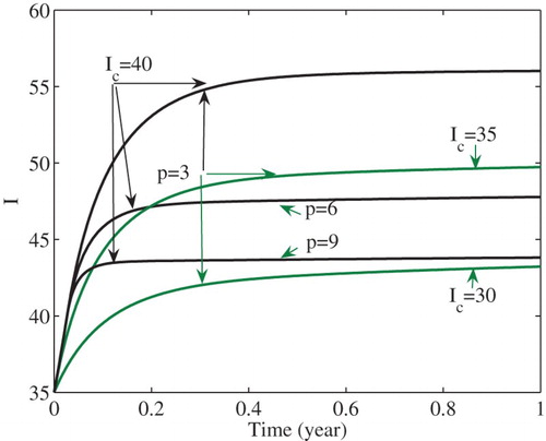
We can illustrate the global stability by numerical simulations. Set $I_c=40$ and the remaining parameters take the same values as in Figure 2. Then $a>a_2=549$. From Remark 1 and Corollary 4.4, the unique endemic equilibrium $E_1$ (see the region $Q_1$ in Figure 1) of model (3(3) $\begin{array}{rl}\frac{\mathrm{d}S}{\mathrm{d}t}& =rS\left(1-\frac{S}{a}\right)-\beta \left(I\right)IS+\gamma I,\\ \frac{\mathrm{d}I}{\mathrm{d}t}& =\beta \left(I\right)IS-(d+ϵ+\gamma )I,\end{array}$(3) ) is globally asymptotically stable. Figure 5 shows that the number I of infections is stabilized at the level $I_1$. In the figure, it is also shown that the number I of infected cases is stabilized at decreased levels as either the intensity p of the media effect increases or the critical number $I_c$ decreases. That is, stronger media effects and/or lower critical numbers lead to a decreased number of infections at the endemic equilibrium $E_1$. In fact, such decreasing effects are also true for all endemic equilibria except $E_{\ast }$.

Figure 5. The number of infected cases is stabilized at decreased levels as either p increases or $I_c$ decreases.

5. Discussion

During a disease spread, only when the number of infected cases and/or the severity of infection are high enough to draw the attention of media and public health organizations, alerts are issued and all related information is brought to the public through media coverage. The information gradually changes public behaviour, which reduces the chance of potential contact infection and eventually helps to curb the disease spread. Fast and dramatic changes in public behaviour can also occur subject to some intensive control measures such as closing school and distancing certain groups of persons. Previous studies have introduced a critical number $I_c$ to be the level for media and health organizations to take action. Functions with jump-discontinuity at $I_c$ were used to describe the changing transmission rate due to the media effect [28, 34, 35]. With the rate functions, media effects on disease outbreaks were studied through compartmental epidemic models. It turns out that proper use of media coverage can curb disease outbreaks [28, 34]. In this paper, following the idea of the critical number $I_c$, we proposed the non-smooth function (2) to describe the transmission rate which is continuous at $I_c$. With this description, change in public behaviour is continuous. Using a susceptible–infected–susceptible model with a logistic growth in the susceptible class, we studied the media effect on the transmission dynamics of an infectious disease in a given region.

Our model analysis shows that without the media effect or with relatively weak effect ($0<p\le 1$), the endemic equilibrium $E_{\ast }$ or $E_1$ (depending on the chosen $I_c$) is globally asymptotically stable. With relatively strong media effect p>1, the model may have up to three endemic equilibria for the chosen critical number $I_c$ in the threshold interval $\mathrm{\Gamma }=[I_c^1,I_c^2]$. Otherwise, the model admits a unique endemic equilibrium (which is globally asymptotically stable, see Figure 1). In the former case, solutions to the model can converge to either one of two stable endemic equilibria (see Figures 2 and 3), depending on initial conditions. That is, bi-stability can occur. To avoid such uncertainty in practice, it is necessary to choose the critical number $I_c$ below the value $I_c^1$. It is worthwhile to point out that the critical values $I_c^1$, $I_c^2$ depend only on the basic reproduction number ${\mathfrak{R}}_0$ and the intensity p of the media effect and hence they are prescribed by the focal disease and the population in the given region. Therefore, it is possible for policymaker to roughly estimate the threshold interval for re-emerged diseases and then choose a reasonable critical number $I_c$ to initiate media coverage.

From the point of view of disease control, early media alerts (i.e. setting a small critical number for $I_c$) and strong media effects (i.e. p>1) are definitely preferable. Our analysis shows that if $I_c<I_{\ast }$, equivalently $a>a_2$, the endemic equilibrium $E_1$ is globally asymptotically stable. However, if $I_c>I_c^2$, model solutions approach the unique equilibrium $E_{\ast }$, causing that media coverage loses its impact on disease transmission. This should be avoided by health policymakers.

Early media alerts and strong effect can decrease the numbers of infected cases at endemic equilibria $I_i$, $i=\mathbf{\text{e}},1,2,3$. For example, as the critical number $I_c$ decreases, or the intensity p of the media effect increases, the number of infected cases can be stabilized at $E_1$ with decreased numbers of cases (see Figure 5). Therefore, properly choosing the critical number and strengthening the media effect can reduce disease prevalence. The analysis of an SEI model also implies that media coverage can reduce the number of infected cases at endemic equilibria [9].

The existence of multiple endemic equilibria was obtained in some previous studies (see e.g. [9, 20]). Using the transmission rate $\beta {\mathrm{e}}^{-mI}$ with media parameter m, Cui et al. [9] found that the model may exhibit periodic oscillations for sufficiently small media effects (small m) and may have multiple endemic equilibria for strong media effects (large m). Unfortunately, the stabilities of the equilibria are not available and hence the solution behaviour is unknown for strong media effects. Media/psychological effects may be also included in the incidence rate in a nonlinear and saturation way such as $k{I}^{2}S/(1+\alpha I^2)$ and simple compartmental models can exhibit complex dynamics. For instance, saddle-node bifurcation, Hopf bifurcation and homocyclic bifurcation can occur in a simple SIR epidemic model with the rate [20]. Therefore, the impact of media coverage on a disease transmission dynamics could be complicated and simplified understandings may even make the disease worse (e.g. [24]). It needs to be further studied from distinct aspects [8].

In order to avoid the complexity of mathematical analysis we assumed that the logistic growth in the susceptible class depends only on the number of the susceptible, instead of the total population size. This is a significant simplification. As an end of the paper, we would like to point out that this simplification is unlikely to change our major qualitative results about the media effect, such as the existence of the threshold interval Γ and bi-stability.

Acknowledgments

The authors thank the editor and the anonymous reviewers for their constructive comments that help to improve the early version of this paper.

Disclosure statement

No potential conflict of interest was reported by the authors.

Additional information

Funding

The work was supported by National Natural Science Foundation of China [No. 11261017, 11371161].

References

- R.M. Anderson, H.C. Jackson, R.M. May, and A.D.M. Smith, Population dynamics of fox rabies in Europe, Nature 289 (1981), pp. 765–771. doi: 10.1038/289765a0
- F. Brauer, Models for the spread of universally fatal diseases, J. Math. Biol. 28 (1990), pp. 451–462. doi: 10.1007/BF00178328
- F. Brauer and C. Castillo-Chavez, Mathematical Models in Population Biology and Epidemiology, Springer, New York, 2001.
- S. Broder and R.C. Gallo, A pathogenic retrovirus (HTLV-III) linked to AIDS, New Engl. J. Med. 311 (1984), pp. 1292–1297. doi: 10.1056/NEJM198411153112006
- S. Busenberg and P. van den Driessche, Analysis of a disease transmission model in a population with varying size, J. Math. Biol. 28 (1990), pp. 257–270. doi: 10.1007/BF00178776
- CDC, H1N1 Flu, Center for Disease Control and Prevention Website. Available at http://www.cdc.gov/h1n1flu/.
- N.S. Chong and R.J. Smith, Modeling avian influenza using Filippov systems to determine culling of infected birds and quarantine, Nonlinear Anal. Real World Appl. 24 (2015), pp. 196–218. doi: 10.1016/j.nonrwa.2015.02.007
- S. Collinson and J.M. Heffernan, Modelling the effects of media during an influenza epidemic, BMC Public Health 14 (2014), pp. 1–10. doi: 10.1186/1471-2458-14-376
- J. Cui, Y. Sun, and H. Zhu, The impact of media on the control of infectious diseases, J. Dynam. Differential Equations 20 (2008), pp. 31–53. doi: 10.1007/s10884-007-9075-0
- J-A. Cui, X. Tao, and H. Zhu, An SIS infection model incorporating media coverage, Rocky Mountain J. Math. 38 (2008), pp. 1323–1334. doi: 10.1216/RMJ-2008-38-5-1323
- H.W. Hethcote, A thousand and one epidemic models, in Frontiers in Mathematical Biology, S.A. Levin, ed., Lecture Notes in Biomathematics, Vol. 100, Springer, Berlin, 1994, pp. 504–515.
- S. Leekha, N.L. Zitterkopf, M.J. Espy, T.F. Smith, R.L. Thompson, and P. Sampathkumar, Duration of influenza: A virus shedding in hospitalized patients and implications for infection control, Infect. Control Hosp. Epidemiol. 28 (2007), pp. 1071–1076. doi: 10.1086/520101
- Y. Liu and J-A. Cui, The impact of media coverage on the dynamics of infectious disease, Int. J. Biomath. 1 (2008), pp. 65–74. doi: 10.1142/S1793524508000023
- R. Liu, J. Wu, and H. Zhu, Media/psychological impact on multiple outbreaks of emerging infectious diseases, Comput. Math. Methods Med. 8 (2007), pp. 153–164. doi: 10.1080/17486700701425870
- Y. Li and J. Cui, The effect of constant and pulse vaccination on SIS epidemic models incorporating media coverage, Commun. Nonlinear Sci. Numer. Simul. 14 (2009), pp. 2353–2365. doi: 10.1016/j.cnsns.2008.06.024
- Y. Li, C. Ma, and J. Cui, The effect of constant and mixed impulsive vaccination on SIS epidemic models incorporating media coverage, Rocky Mountain J. Math. 38 (2008), pp. 1437–1455. doi: 10.1216/RMJ-2008-38-5-1437
- J. Pang and J. Cui, An SIRS epidemiological model with nonlinear incidence rate incorporating media coverage, Second International Conference on Information and Computing Science, USA, IEEE, 2009, pp. 116–119.
- L. Perko, Differential Equations and Dynamical Systems, Springer-Verlag, New York, 1996.
- M.S. Rahman and M.L. Rahman, Media and education play a tremendous role in mounting AIDS awareness among married couples in Bangladesh, AIDS Res. Therapy 4 (2007), pp. 1–7. doi: 10.1016/0005-7967(66)90037-4
- S. Ruan and W. Wang, Dynamical behavior of an epidemic model with a nonlinear incidence rate, J. Differential Equations 188 (2003), pp. 135–163. doi: 10.1016/S0022-0396(02)00089-X
- F. Schweitzer and R. Mach, The epidemics of donations: Logistic growth and power-laws, PLoS One 3 (2008), p. e1458. doi: 10.1371/journal.pone.0001458
- A.M. Spagnuolo, M. Shillor, L. Kingsland, A. Thatcher, M. Toeniskoetter, and B. Wood, A logistic delay differential equation model for Chagas disease with interrupted spraying schedules, J. Biol. Dynam. 6 (2012), pp. 377–394. doi: 10.1080/17513758.2011.587896
- C. Sun, W. Yang, J. Arino, and K. Khan, Effect of media-induced social distancing on disease transmission in a two patch setting, Math. Biosci. 230 (2011), pp. 87–95. doi: 10.1016/j.mbs.2011.01.005
- J.M. Tchuenche, N. Dube, C.P. Bhunu, R.J. Smith, and C.T. Bauch, The impact of media coverage on the transmission dynamics of human influenza, BMC Public Health 11 (2011), pp. 1–16. doi: 10.1186/1471-2458-11-1
- S.M. Tracht, S.Y. Del Valle, J.M. Hyman, and D.A. Carter, Mathematical modeling of the effectiveness of facemasks in reducing the spread of novel influenza A (H1N1), PLoS One 5 (2010), p. e9018. doi: 10.1371/journal.pone.0009018
- V.I. Utkin, Sliding Modes in Control and Optimization, Springer-Verlag, Berlin, 1992.
- W. Wang, Backward bifurcation of an epidemic model with treatment, Math. Biosci. 201 (2006), pp. 58–71. doi: 10.1016/j.mbs.2005.12.022
- A. Wang and Y. Xiao, A Filippov system describing media effects on the spread of infectious diseases, Nonlinear Anal. Hybr. Syst. 11 (2014), pp. 84–97. doi: 10.1016/j.nahs.2013.06.005
- J-J. Wang, J-Z. Zhang, and Z. Jin, Analysis of an SIR model with bilinear incidence rate, Nonlinear Anal. Real World Appl. 11 (2010), pp. 2390–2402. doi: 10.1016/j.nonrwa.2009.07.012
- L.F. White, J. Wallinga, L. Finelli, C. Reed, S. Riley, M. Lipsitch, and M. Pagano, Estimation of the reproductive number and the serial interval in early phase of the 2009 influenza A/H1N1 pandemic in the USA, Influenza Other Respir. Viruses 3 (2009), pp. 267–276. doi: 10.1111/j.1750-2659.2009.00106.x
- WHO, Avian influenza A(H7N9) overview, 2013. Available at http://www.who.int/influenza/human_animal_interface/influenza_h7n9/WHA_H7N9_update_KeijiFukuda_21May13.pdf?ua=1.
- WHO, Situation Report 1 Ebola virus disease, Guinea, 2014. Available at http://www.afro.who.int/en/clusters-a-programmes/dpc/epidemic-a-pandemic-alert-and-response/sitreps/4070-sitrep-1-ebola-guinea-28-march-2014.html.
- D. Xiao and S. Ruan, Global analysis of an epidemic model with nonmonotone incidence rate, Math. Biosci. 208 (2007), pp. 419–429. doi: 10.1016/j.mbs.2006.09.025
- Y. Xiao, X. Xu, and S. Tang, Sliding mode control of outbreaks of emerging infectious diseases, Bull. Math. Biol. 74 (2012), pp. 2403–2422. doi: 10.1007/s11538-012-9758-5
- Y. Xiao, S. Tang, and J. Wu, Media impact switching surface during an infectious disease outbreak, Scientific Reports, 5 (2015), article 7838.
- X. Zhang and L. Chen, The periodic solution of a class of epidemic models, Comput. Math. Appl. 38 (1999), pp. 61–71. doi: 10.1016/S0898-1221(99)00206-0
- Z. Zhang, T. Ding, W. Huang, and Z. Dong, Qualitative Theory of Differential Equations, Vol. 101, Amer. Math. Soc., Providence, 1992.
- J. Zu and L. Wang, Periodic solutions for a seasonally forced SIR model with impact of media coverage, Adv. Difference Equ. 2015 (2015), pp. 1–10. doi:10.1186/s13662-015-0477-8.