Finite-time Lyapunov exponents and metabolic control coefficients for threshold detection of stimulus–response curves

ABSTRACT

In biochemical networks transient dynamics plays a fundamental role, since the activation of signalling pathways is determined by thresholds encountered during the transition from an initial state (e.g. an initial concentration of a certain protein) to a steady-state. These thresholds can be defined in terms of the inflection points of the stimulus–response curves associated to the activation processes in the biochemical network. In the present work, we present a rigorous discussion as to the suitability of finite-time Lyapunov exponents and metabolic control coefficients for the detection of inflection points of stimulus–response curves with sigmoidal shape.

KEYWORDS:

• Finite-time Lyapunov spectrum
• transient dynamics
• sigmoidal response curve
• nonautonomous dynamical system

2010 MATHEMATICS SUBJECT CLASSIFICATION:

• 37N25

1. Introduction

The study of long-term dynamics of mathematical models describing biological phenomena has received considerable attention in the past, with particular attention to steady-states and oscillatory solutions. Many methods for studying steady-state signals in biological models based on ordinary differential equations (ODE) have been developed (see, e.g. [10,15] and the references therein). However, transient effects can play a fundamental role as well. For instance, in biological networks the sequence of cellular processes can be affected by the short-term behaviour of time-varying signals, as is observed, for example, in cell apoptosis [1], transient pathology [14] or phytotransduction [18]. Typically, the activation of signal transduction pathways is determined by thresholds encountered during the transition from an initial state (e.g. an initial concentration of a certain protein) to a steady state. These thresholds can be defined in terms of the inflection points of the stimulus–response curves associated to the activation processes in the biochemical network, such as cell differentiation, apoptosis, DNA damage response, etc. In our investigation, such stimulus–response curves will be assumed to have a sigmoidal shape (to be formally defined later), as is common in the determination of thresholds in biological networks [3,4].

Previous investigations have focused on network properties leading to sigmoidal stimulus–response curves in the steady-state dynamics [17,21]. For small biological networks, stimulus–response curves of the transient and long-term dynamics can be studied in detail, leading to a straightforward identification of putative thresholds. However, in larger biochemical networks the identification of putative thresholds can be more challenging, in particular in the case when the network components present sigmoidal response curves during different time intervals. Therefore, it is essential to develop quantitative measures that are suitable for the identification of putative thresholds during the transient behaviour of biological networks.

Examples of quantitative measures to characterize the transient dynamics of signal transduction pathways include metabolic control coefficients (MCC) [14] and finite-time Lyapunov exponents (FTLE) [1,19]. In fact, MCC were originally introduced to study the dynamics near steady states (see [10,15]), but then proved to be still effective for the analysis of transient behaviour. Ingalls and Sauro [14] extended the steady-state results of MCC to special types of dynamic response, e.g. periodic behaviour and trajectories near stable steady states, by measuring time-varying sensitivities along arbitrary solutions. Aldridge et al. [1] employed FTLE to identify phase-space domains of high sensitivity to initial conditions, which enables the identification of separatrices that quantitatively characterize network responses in terms of initial conditions determining cell death or survival.

Rateitschak and Wolkenhauer [19] suggested that FTLE can be used to reliably identify thresholds as inflection points of stimulus–response curves in transient dynamics, while MCC are more suitable for comparing the amplitude of different thresholds. Nevertheless, their conclusions are based on numerical simulations of three examples and mathematical proofs of their claims are missing. In the present paper, we tackle the question whether FTLE and MCC are indeed reliable measures for detecting thresholds in stimulus–response curves with sigmoidal shape, and if so, under what conditions meaningful estimates of such thresholds can be obtained.

The paper is structured as follows. In Section 2, we introduce the basic mathematical framework required for our study. Then, our main objects of interest, FTLE and MCC, are defined in Section 3. There, we derive one of the main results of the paper, which establishes a connection between FTLE and MCC. In Section 4, the concept of (sigmoidal) stimulus–response curve is introduced, and the main concern here is to investigate the suitability of both FTLE and MCC to detect inflection points of stimulus–response curves. The main results of the paper are illustrated by numerical examples. Some concluding remarks are presented at the end of the paper.

2. Basic setup and notation

Throughout this paper, we consider the nonautonomous differential equation (1) $x^{\prime }\left(t\right)=f(t,x(t\left)\right),t\in I:=[t_0,t_0+T_0],$(1) where $t_0\in \mathbb{R}$, $T_0\in {\mathbb{R}}^{+}$ and $f:I\times {\mathbb{R}}^d\to {\mathbb{R}}^d$ is a continuous function and continuously differentiable in the second argument. Let $\varphi :I\times I\times {\mathbb{R}}^d\to {\mathbb{R}}^d$ be the solution operator of Equation (1(1) $x^{\prime }\left(t\right)=f(t,x(t\left)\right),t\in I:=[t_0,t_0+T_0],$(1) ), i.e. $t\mapsto \varphi (t,\tau ,\xi )$ solves Equation (1(1) $x^{\prime }\left(t\right)=f(t,x(t\left)\right),t\in I:=[t_0,t_0+T_0],$(1) ) subject to the initial condition $x\left(\tau \right)=\xi$. Here, it is assumed that for every $(\tau ,\xi )\in I\times {\mathbb{R}}^d$, $\varphi (\cdot ,\tau ,\xi )$ exists on the whole interval I. Furthermore, denote by $P:{\mathbb{R}}^d\times (0,T_0]\to {\mathbb{R}}^d$ the time-T map (2) $P(x,T):=\varphi (t_0+T,t_0,x),x\in {\mathbb{R}}^d,T\in (0,T_0].$(2)

Moreover, to study the evolution of small perturbations near a solution $\overline{x}\left(t\right):=\varphi (t,t_0,x)$, $t\in I$, of Equation (1(1) $x^{\prime }\left(t\right)=f(t,x(t\left)\right),t\in I:=[t_0,t_0+T_0],$(1) ), we consider the variational equation along $\overline{x}\left(t\right)$ (3) $y^{\prime }\left(t\right)=\frac{\mathrm{\partial }f}{\mathrm{\partial }x}(t,\varphi (t,t_0,x\left)\right)y\left(t\right),y\left(t\right)\in {\mathbb{R}}^d,t\in I.$(3) We further denote by $\mathrm{\Phi }:I\times I\times {\mathbb{R}}^d\to {\mathbb{R}}^{d\times d}$ the transition matrix of the linear system (3(3) $y^{\prime }\left(t\right)=\frac{\mathrm{\partial }f}{\mathrm{\partial }x}(t,\varphi (t,t_0,x\left)\right)y\left(t\right),y\left(t\right)\in {\mathbb{R}}^d,t\in I.$(3) ), i.e. for any $y_0\in {\mathbb{R}}^d$, $t\mapsto \mathrm{\Phi }(t,t_0,x)y_0$ solves the problem (3(3) $y^{\prime }\left(t\right)=\frac{\mathrm{\partial }f}{\mathrm{\partial }x}(t,\varphi (t,t_0,x\left)\right)y\left(t\right),y\left(t\right)\in {\mathbb{R}}^d,t\in I.$(3) ) subject to the initial condition $y\left(t_0\right)=y_0$.

Similarly to Equation (2(2) $P(x,T):=\varphi (t_0+T,t_0,x),x\in {\mathbb{R}}^d,T\in (0,T_0].$(2) ), we define the time-T transition matrix $\mathrm{\Psi }:{\mathbb{R}}^d\times (0,T_0]\to {\mathbb{R}}^{d\times d}$ of Equation (3(3) $y^{\prime }\left(t\right)=\frac{\mathrm{\partial }f}{\mathrm{\partial }x}(t,\varphi (t,t_0,x\left)\right)y\left(t\right),y\left(t\right)\in {\mathbb{R}}^d,t\in I.$(3) ) by (4) $\mathrm{\Psi }(x,T):=\mathrm{\Phi }(t_0+T,t_0,x),x\in {\mathbb{R}}^d,T\in (0,T_0].$(4) Due to Equations (2(2) $P(x,T):=\varphi (t_0+T,t_0,x),x\in {\mathbb{R}}^d,T\in (0,T_0].$(2) ) and (4(4) $\mathrm{\Psi }(x,T):=\mathrm{\Phi }(t_0+T,t_0,x),x\in {\mathbb{R}}^d,T\in (0,T_0].$(4) ) and the relation $\frac{\mathrm{\partial }\varphi }{\mathrm{\partial }x}(t,t_0,x)=\mathrm{\Phi }(t,t_0,x),t\in I,x\in {\mathbb{R}}^d,$ it follows immediately that (5) $\frac{\mathrm{\partial }P}{\mathrm{\partial }x}(x,T)=\mathrm{\Psi }(x,T),x\in {\mathbb{R}}^d,T\in (0,T_0].$(5)

To conclude this preliminary part, we introduce the symbol $G_{d,k}$ to denote the Grassmann manifold of all k-dimensional subspaces of ${\mathbb{R}}^d$.

3. FTLE and their relation to MCC

Denote by ${\mu }_1\left(A\right)\ge \cdots \ge {\mu }_d\left(A\right)\ge 0$ the ordered singular values of a matrix $A\in {\mathbb{R}}^{d\times d}$, which are defined as the square roots of the eigenvalues of $A^{T}A$ [13]. The FTLE associated with a solution $\overline{x}\left(t\right)=\varphi (t,t_0,x)$ of Equation (1(1) $x^{\prime }\left(t\right)=f(t,x(t\left)\right),t\in I:=[t_0,t_0+T_0],$(1) ) on the interval $[t_0,t_0+T]\subset I$ are defined as [7–9] (6) ${\lambda }_k(x,T):=\frac{1}{T}\ln \left({\mu }_k\right(\mathrm{\Psi }(x,T)\left)\right),x\in {\mathbb{R}}^d,T\in (0,T_0],k=1,\dots ,d,$(6) see also [20]. In our discussion, it will be convenient to use the following alternative expressions for the FTLE (7) ${\lambda }_k(x,T)=\frac{1}{T}\ln \left(\underset{U\in G_{d,d-k+1}}{inf}\underset{\begin{array}{c}u\in U\\ u\ne 0\end{array}}{sup}\frac{{∥\mathrm{\Psi }(x,T)u∥}_2}{{∥u∥}_2}\right)=\frac{1}{T}\ln \left(\underset{U\in G_{d,k}}{sup}\underset{\begin{array}{c}u\in U\\ u\ne 0\end{array}}{inf}\frac{{∥\mathrm{\Psi }(x,T)u∥}_2}{{∥u∥}_2}\right),$(7) for all $k=1,\dots ,d$, $x\in {\mathbb{R}}^d$ and $T\in (0,T_0]$, where ${∥\cdot ∥}_2$ stands for the Euclidean norm in ${\mathbb{R}}^d$. The formulae (7(7) ${\lambda }_k(x,T)=\frac{1}{T}\ln \left(\underset{U\in G_{d,d-k+1}}{inf}\underset{\begin{array}{c}u\in U\\ u\ne 0\end{array}}{sup}\frac{{∥\mathrm{\Psi }(x,T)u∥}_2}{{∥u∥}_2}\right)=\frac{1}{T}\ln \left(\underset{U\in G_{d,k}}{sup}\underset{\begin{array}{c}u\in U\\ u\ne 0\end{array}}{inf}\frac{{∥\mathrm{\Psi }(x,T)u∥}_2}{{∥u∥}_2}\right),$(7) ) are a direct consequence of the Courant–Fischer theorem for singular values [13].

The largest FTLE ${\lambda }_1(x,T)$ can be interpreted as a measure of the maximal average exponential separation rate between the solution $\overline{x}(\cdot )$ starting at x and neighbouring trajectories with initial point infinitesimally close to x, over the time interval $[t_0,t_0+T]$, see [8].

Example 3.1.

Consider the planar system (8) $\begin{array}{rl}{x}_1^{\prime }\left(t\right)& =\kappa x_1\left(t\right),\\ x_2^{\prime }\left(t\right)& =g\left(x_1\right(t\left)\right)-x_2\left(t\right),\end{array}$(8) with $t\ge 0$ and (9) $g\left(\nu \right):=\frac{{\nu }^{{\eta }_{\mathrm{H}}}}{{\rho }_{\mathrm{H}}^{{\eta }_{\mathrm{H}}}+{\nu }^{{\eta }_{\mathrm{H}}}},\nu \ge 0.$(9)

System (8(8) $\begin{array}{rl}{x}_1^{\prime }\left(t\right)& =\kappa x_1\left(t\right),\\ x_2^{\prime }\left(t\right)& =g\left(x_1\right(t\left)\right)-x_2\left(t\right),\end{array}$(8) ) can be interpreted in a biological framework as follows. The first equation describes an exponential growth without saturation, which may represent the reproduction behaviour of a certain organism in a favourable environment. The function $x_2\left(t\right)$, $t\ge 0$, can be associated with the population density of a second organism that decays exponentially in absence of the first. According to Equation (8(8) $\begin{array}{rl}{x}_1^{\prime }\left(t\right)& =\kappa x_1\left(t\right),\\ x_2^{\prime }\left(t\right)& =g\left(x_1\right(t\left)\right)-x_2\left(t\right),\end{array}$(8) ), the only source term of the second organism is given by the function g, which is the well-known Hill function. It was first introduced by Hill [12] at the beginning of the twentieth century to describe the relationship between oxygen tension and the saturation of haemoglobin with oxygen, under equilibrium conditions. The Hill function has been used in numerous biological applications and beyond, in particular to describe biological phenomena exhibiting sigmoidal kinetics [3,6,11].

Throughout this paper, we will consider system (8(8) $\begin{array}{rl}{x}_1^{\prime }\left(t\right)& =\kappa x_1\left(t\right),\\ x_2^{\prime }\left(t\right)& =g\left(x_1\right(t\left)\right)-x_2\left(t\right),\end{array}$(8) ) for the case $\kappa =1$, ${\rho }_{\mathrm{H}}=1$ and ${\eta }_{\mathrm{H}}=2$. Let us compute the FTLE associated with a solution of Equation (8(8) $\begin{array}{rl}{x}_1^{\prime }\left(t\right)& =\kappa x_1\left(t\right),\\ x_2^{\prime }\left(t\right)& =g\left(x_1\right(t\left)\right)-x_2\left(t\right),\end{array}$(8) ) starting at $x:=(x_1,x_2)\in {\mathbb{R}}^{+}\times {\mathbb{R}}^{+}$ defined over the interval $[0,T]$. The time-T map of Equation (8(8) $\begin{array}{rl}{x}_1^{\prime }\left(t\right)& =\kappa x_1\left(t\right),\\ x_2^{\prime }\left(t\right)& =g\left(x_1\right(t\left)\right)-x_2\left(t\right),\end{array}$(8) ) has the explicit form (cf. (2(2) $P(x,T):=\varphi (t_0+T,t_0,x),x\in {\mathbb{R}}^d,T\in (0,T_0].$(2) )) (10) $P(x,T)=\left(\begin{array}{c}{x}_1{e}^T\\ e^{-T}\left(e^T+x_2-1-\frac{\arctan \left(x_1{e}^T\right)-\arctan \left(x_1\right)}{x_1}\right)\end{array}\right).$(10) With this expression, we can compute the time-T transition matrix via Equation (5(5) $\frac{\mathrm{\partial }P}{\mathrm{\partial }x}(x,T)=\mathrm{\Psi }(x,T),x\in {\mathbb{R}}^d,T\in (0,T_0].$(5) ), which gives (11) $\mathrm{\Psi }(x,T)=\left(\begin{array}{cc}{e}^T& 0\\ \frac{1}{x_1(e^{2T}{x}_1^2+1)}-\frac{e^{-T}(x_1+(x_1^2+1\left)\right(\arctan \left(x_1\right)-\arctan \left(x_1{e}^T\right)\left)\right)}{x_1^2(x_1^2+1)}& e^{-T}\end{array}\right).$(11)

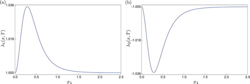
In Figure 1 we show the behaviour of the corresponding FTLE as $x_1$ varies, for T=1 fixed. In this example, ${\lambda }_{1,2}$ can be computed explicitly by combining Equations (11(11) $\mathrm{\Psi }(x,T)=\left(\begin{array}{cc}{e}^T& 0\\ \frac{1}{x_1(e^{2T}{x}_1^2+1)}-\frac{e^{-T}(x_1+(x_1^2+1\left)\right(\arctan \left(x_1\right)-\arctan \left(x_1{e}^T\right)\left)\right)}{x_1^2(x_1^2+1)}& e^{-T}\end{array}\right).$(11) ) and (6(6) ${\lambda }_k(x,T):=\frac{1}{T}\ln \left({\mu }_k\right(\mathrm{\Psi }(x,T)\left)\right),x\in {\mathbb{R}}^d,T\in (0,T_0],k=1,\dots ,d,$(6) ). In this case, ${\lambda }_{1,2}$ are $x_2$-independent, as can be seen from Equation (11(11) $\mathrm{\Psi }(x,T)=\left(\begin{array}{cc}{e}^T& 0\\ \frac{1}{x_1(e^{2T}{x}_1^2+1)}-\frac{e^{-T}(x_1+(x_1^2+1\left)\right(\arctan \left(x_1\right)-\arctan \left(x_1{e}^T\right)\left)\right)}{x_1^2(x_1^2+1)}& e^{-T}\end{array}\right).$(11) ).

Figure 1. FTLE computed for system (8(8) $\begin{array}{rl}{x}_1^{\prime }\left(t\right)& =\kappa x_1\left(t\right),\\ x_2^{\prime }\left(t\right)& =g\left(x_1\right(t\left)\right)-x_2\left(t\right),\end{array}$(8) ) at T=1.

Let us now introduce another quantity that, together with FTLE, will play a central role in our discussion. In the context of metabolic control analysis [11], one of the main concerns is to analyse the role of a specific substance in reactions taking place in living cells. Due to the high number of variables and regulatory interrelations involved in such processes, different approaches have been developed in order to quantitatively characterize the various metabolic pathways determining fluxes and metabolite concentrations. One way to deal with this issue is by means of the so-called MCC, defined as (cf. [19]) (12) $c_{ij}(x,T):=\frac{\mathrm{\partial }\log P_i}{\mathrm{\partial }\log x_j}(x,T):=\frac{x_j}{P_i(x,T)}\frac{\mathrm{\partial }{P}_i}{\mathrm{\partial }{x}_j}(x,T),i,j=1,\dots d,$(12) for $(x,T)\in {\mathbb{R}}^d\times (0,T_0]$ such that $P_i(x,T)\ne 0$, where $x=(x_1,\dots ,x_d)$ and $P(x,T)=\left(P_1\right(x,T),\dots ,$ $P_d(x,T))$. The matrix $C(x,T):=\left(c_{ij}\right(x,T){)}_{i,j=1,\dots ,d}$ is referred to as the metabolic control matrix. The coefficient $c_{ij}(x,T)$ gives a (dimensionless) local measure of the relative change in the ith output of the system with respect to an infinitesimal relative change in the jth component of the initial conditions, in the vicinity of a reference state x. The MCC can also be interpreted as a sensitivity measure (with respect to initial conditions), which is a concept widely used in engineering applications [2].

For $x=(x_1,\dots ,x_d)\in {\mathbb{R}}^d$, let us denote by $\mathrm{diag}\left(x\right)\in {\mathbb{R}}^{d\times d}$ a diagonal matrix with entries $x_1,\dots ,x_d$ in the diagonal. A straightforward computation shows that (13) $\mathrm{\Psi }(x,T)=\mathrm{diag}\left(P\right(x,T\left)\right)C(x,T)\mathrm{diag}(x{)}^{-1}$(13) holds for all $T\in (0,T_0]$ and $x\in {\mathbb{R}}^d$ with $x_i\ne 0$, $i=1,\dots ,d$. The expression (13(13) $\mathrm{\Psi }(x,T)=\mathrm{diag}\left(P\right(x,T\left)\right)C(x,T)\mathrm{diag}(x{)}^{-1}$(13) ) establishes a clear connection between the time-T transition matrix $\mathrm{\Psi }(x,T)$ and the metabolic control matrix $C(x,T)$. This relation motivates the main result of the present section shown below.

Theorem 3.1.

Suppose that there exist constants 0<m<M such that the set $\mathrm{\Omega }:=\{x\in {\mathbb{R}}^d:m\le \left|x_i\right|\le M\mathrm{and}m\le \left|P_i(x,T)\right|\le M\mathrm{for}\mathrm{all}T\in (0,T_0]\mathrm{and}i=1,\dots ,d\}$ is not empty. Then the following estimates (14) $\left|{\lambda }_k(x,T)-\frac{1}{T}\ln \left({\mu }_k\right(C(x,T)\left)\right)\right|\le \frac{1}{T}\ln \left(\frac{M}{m}\right),k=1,\dots ,d,$(14) hold for all $x\in \mathrm{\Omega }$ and $T\in (0,T_0]$.

Proof.

Define a family of linear operators $H_x:{\mathbb{R}}^d\to {\mathbb{R}}^d$, $u\mapsto H_x\left(u\right):=\mathrm{diag}(x{)}^{-1}u$, parametrized by $x\in \mathrm{\Omega }$. Note that $H_x(\cdot )$ is invertible for all $x\in \mathrm{\Omega }$ and (15) $\begin{array}{rl}{∥H_x\left(u\right)∥}_2& \le \frac{1}{m}{∥u∥}_2,\end{array}$(15) (16) $\begin{array}{rl}{∥H_x^{-1}\left(v\right)∥}_2& \le M{∥v∥}_2,\end{array}$(16) (17) $\begin{array}{rl}{∥\mathrm{diag}\left(P\right(x,T\left)\right)∥}_2& \le M,\end{array}$(17) (18) $\begin{array}{rl}{∥\mathrm{diag}\left(P\right(x,T){)}^{-1}∥}_2& \le \frac{1}{m},\end{array}$(18) hold for all $u,v\in {\mathbb{R}}^d$ and $(x,T)\in \mathrm{\Omega }\times (0,T_0]$. In order to prove Equation (14(14) $\left|{\lambda }_k(x,T)-\frac{1}{T}\ln \left({\mu }_k\right(C(x,T)\left)\right)\right|\le \frac{1}{T}\ln \left(\frac{M}{m}\right),k=1,\dots ,d,$(14) ), we will use the formulae introduced in Equation (7(7) ${\lambda }_k(x,T)=\frac{1}{T}\ln \left(\underset{U\in G_{d,d-k+1}}{inf}\underset{\begin{array}{c}u\in U\\ u\ne 0\end{array}}{sup}\frac{{∥\mathrm{\Psi }(x,T)u∥}_2}{{∥u∥}_2}\right)=\frac{1}{T}\ln \left(\underset{U\in G_{d,k}}{sup}\underset{\begin{array}{c}u\in U\\ u\ne 0\end{array}}{inf}\frac{{∥\mathrm{\Psi }(x,T)u∥}_2}{{∥u∥}_2}\right),$(7) ) for the computation of FTLE as follows. Choose $U\in G_{d,k}$ for some $1\le k\le d$. By Equations (13(13) $\mathrm{\Psi }(x,T)=\mathrm{diag}\left(P\right(x,T\left)\right)C(x,T)\mathrm{diag}(x{)}^{-1}$(13) ), (15(15) $\begin{array}{rl}{∥H_x\left(u\right)∥}_2& \le \frac{1}{m}{∥u∥}_2,\end{array}$(15) ) and (17(17) $\begin{array}{rl}{∥\mathrm{diag}\left(P\right(x,T\left)\right)∥}_2& \le M,\end{array}$(17) ) it follows for $0\ne u\in U$ that (19) $\begin{array}{rl}\frac{{∥\mathrm{\Psi }(x,T)u∥}_2}{{∥u∥}_2}& =\frac{{∥\mathrm{diag}\left(P\right(x,T\left)\right)C(x,T)\mathrm{diag}(x{)}^{-1}u∥}_2}{{∥u∥}_2}\\ & =\frac{{∥\mathrm{diag}\left(P\right(x,T\left)\right)C(x,T)H_x\left(u\right)∥}_2}{{∥H_x\left(u\right)∥}_2}\frac{{∥H_x\left(u\right)∥}_2}{{∥u∥}_2}\\ & \le \frac{1}{m}\frac{{∥\mathrm{diag}\left(P\right(x,T\left)\right)C(x,T)H_x\left(u\right)∥}_2}{{∥H_x\left(u\right)∥}_2}\\ & \le \frac{1}{m}\frac{{∥C(x,T)H_x\left(u\right)∥}_2}{{∥H_x\left(u\right)∥}_2}{∥\mathrm{diag}\left(P\right(x,T\left)\right)∥}_2\\ & \le \frac{M}{m}\frac{{∥C(x,T)H_x\left(u\right)∥}_2}{{∥H_x\left(u\right)∥}_2}.\end{array}$(19) Introducing $v:=H_x\left(u\right)$ in Equation (19(16) $\begin{array}{rl}{∥H_x^{-1}\left(v\right)∥}_2& \le M{∥v∥}_2,\end{array}$(16) ) and taking the infimum over all $0\ne u\in U$ yield $\underset{\begin{array}{c}u\in U\\ u\ne 0\end{array}}{inf}\frac{{∥\mathrm{\Psi }(x,T)u∥}_2}{{∥u∥}_2}\le \frac{M}{m}\underset{\begin{array}{c}v\in H_x\left(U\right)\\ v\ne 0\end{array}}{inf}\frac{{∥C(x,T)v∥}_2}{{∥v∥}_2}.$ Next, after taking the supremum over all $U\in G_{d,k}$, we arrive at $\underset{U\in G_{d,k}}{sup}\underset{\begin{array}{c}u\in U\\ u\ne 0\end{array}}{inf}\frac{{∥\mathrm{\Psi }(x,T)u∥}_2}{{∥u∥}_2}\le \frac{M}{m}\underset{U\in G_{d,k}}{sup}\underset{\begin{array}{c}v\in H_x\left(U\right)\\ v\ne 0\end{array}}{inf}\frac{{∥C(x,T)v∥}_2}{{∥v∥}_2}.$ Due to the fact that for any $V\in G_{d,k}$ there exists a $U\in G_{d,k}$ such that $V=H_x\left(U\right)$, we can write the last inequality as $\underset{U\in G_{d,k}}{sup}\underset{\begin{array}{c}u\in U\\ u\ne 0\end{array}}{inf}\frac{{∥\mathrm{\Psi }(x,T)u∥}_2}{{∥u∥}_2}\le \frac{M}{m}\underset{V\in G_{d,k}}{sup}\underset{\begin{array}{c}v\in V\\ v\ne 0\end{array}}{inf}\frac{{∥C(x,T)v∥}_2}{{∥v∥}_2}.$ By using formula (7(7) ${\lambda }_k(x,T)=\frac{1}{T}\ln \left(\underset{U\in G_{d,d-k+1}}{inf}\underset{\begin{array}{c}u\in U\\ u\ne 0\end{array}}{sup}\frac{{∥\mathrm{\Psi }(x,T)u∥}_2}{{∥u∥}_2}\right)=\frac{1}{T}\ln \left(\underset{U\in G_{d,k}}{sup}\underset{\begin{array}{c}u\in U\\ u\ne 0\end{array}}{inf}\frac{{∥\mathrm{\Psi }(x,T)u∥}_2}{{∥u∥}_2}\right),$(7) ) for the computation of FTLE we obtain (20) ${\lambda }_k(x,T)-\frac{1}{T}\ln \left({\mu }_k\right(C(x,T)\left)\right)\le \frac{1}{T}\ln \left(\frac{M}{m}\right),k=1,\dots ,d,$(20) for all $(x,T)\in \mathrm{\Omega }\times (0,T_0]$. Following a similar argument allows us to show for $0\ne u\in U$ that (see Equations (16(16) $\begin{array}{rl}{∥H_x^{-1}\left(v\right)∥}_2& \le M{∥v∥}_2,\end{array}$(16) ) and (18(18) $\begin{array}{rl}{∥\mathrm{diag}\left(P\right(x,T){)}^{-1}∥}_2& \le \frac{1}{m},\end{array}$(18) )) (21) $\begin{array}{rl}\frac{{∥\mathrm{\Psi }(x,T)u∥}_2}{{∥u∥}_2}& =\frac{{∥\mathrm{diag}\left(P\right(x,T\left)\right)C(x,T)v∥}_2}{{∥H_x^{-1}\left(v\right)∥}_2}\\ & \ge \frac{1}{{∥\mathrm{diag}\left(P\right(x,T){)}^{-1}∥}_2}\frac{{∥C(x,T)v∥}_2}{{∥v∥}_2}\frac{{∥v∥}_2}{{∥H_x^{-1}\left(v\right)∥}_2}\\ & \ge \frac{m}{M}\frac{{∥C(x,T)v∥}_2}{{∥v∥}_2}.\end{array}$(21) Applying formula (7(7) ${\lambda }_k(x,T)=\frac{1}{T}\ln \left(\underset{U\in G_{d,d-k+1}}{inf}\underset{\begin{array}{c}u\in U\\ u\ne 0\end{array}}{sup}\frac{{∥\mathrm{\Psi }(x,T)u∥}_2}{{∥u∥}_2}\right)=\frac{1}{T}\ln \left(\underset{U\in G_{d,k}}{sup}\underset{\begin{array}{c}u\in U\\ u\ne 0\end{array}}{inf}\frac{{∥\mathrm{\Psi }(x,T)u∥}_2}{{∥u∥}_2}\right),$(7) ) to (21(18) $\begin{array}{rl}{∥\mathrm{diag}\left(P\right(x,T){)}^{-1}∥}_2& \le \frac{1}{m},\end{array}$(18) ) yields (22) ${\lambda }_k(x,T)-\frac{1}{T}\ln \left({\mu }_k\right(C(x,T)\left)\right)\ge -\frac{1}{T}\ln \left(\frac{M}{m}\right),k=1,\dots ,d,$(22) for all $(x,T)\in \mathrm{\Omega }\times (0,T_0]$. Combining Equations (20(17) $\begin{array}{rl}{∥\mathrm{diag}\left(P\right(x,T\left)\right)∥}_2& \le M,\end{array}$(17) ) and (22(19) $\begin{array}{rl}\frac{{∥\mathrm{\Psi }(x,T)u∥}_2}{{∥u∥}_2}& =\frac{{∥\mathrm{diag}\left(P\right(x,T\left)\right)C(x,T)\mathrm{diag}(x{)}^{-1}u∥}_2}{{∥u∥}_2}\\ & =\frac{{∥\mathrm{diag}\left(P\right(x,T\left)\right)C(x,T)H_x\left(u\right)∥}_2}{{∥H_x\left(u\right)∥}_2}\frac{{∥H_x\left(u\right)∥}_2}{{∥u∥}_2}\\ & \le \frac{1}{m}\frac{{∥\mathrm{diag}\left(P\right(x,T\left)\right)C(x,T)H_x\left(u\right)∥}_2}{{∥H_x\left(u\right)∥}_2}\\ & \le \frac{1}{m}\frac{{∥C(x,T)H_x\left(u\right)∥}_2}{{∥H_x\left(u\right)∥}_2}{∥\mathrm{diag}\left(P\right(x,T\left)\right)∥}_2\\ & \le \frac{M}{m}\frac{{∥C(x,T)H_x\left(u\right)∥}_2}{{∥H_x\left(u\right)∥}_2}.\end{array}$(19) ) shows the validity of the inequality (14(14) $\left|{\lambda }_k(x,T)-\frac{1}{T}\ln \left({\mu }_k\right(C(x,T)\left)\right)\right|\le \frac{1}{T}\ln \left(\frac{M}{m}\right),k=1,\dots ,d,$(14) ).

Theorem 3.1 provides an estimate between FTLE and a logarithmic quantity given in terms of the metabolic control matrix defined before. In fact, the scalar (23) $\zeta (x,T):=\frac{1}{T}\ln \left({\mu }_1\right(C(x,T)\left)\right),x\in {\mathbb{R}}^d,T\in (0,T_0],$(23) is the so-called relative instability exponent, which is introduced by Rateitschak and Wolkenhauer [19] to measure the largest relative change in the system response when the initial conditions are perturbed.

4. Sigmoidal stimulus–response curves

The characterization of the input–output relation in biological networks is commonly done via the so-called stimulus–response curves, in which a scalar output is plotted against a scalar input of the network at a fixed time. In our mathematical framework, such curves can be defined as the family of functions (24) $s_{ij}(x_j,T):=P_i(x_1,\dots ,x_j,\dots ,x_d,T),x_j\in \mathbb{R},T\in (0,T_0],i,j=1,\dots ,d,$(24) where all components of $x=(x_1,\dots ,x_j,\dots ,x_d)$ but $x_j$ are assumed to be fixed.

In practice, stimulus–response curves are oftentimes strictly monotone (increasing or decreasing [11,16]), meaning that their first derivative with respect to the input $x_j$ does not change sign on suitably chosen intervals. Another common feature of stimulus–response curves is their sigmoidal form [3], characterized by a bell-shaped first derivative, as will be made precise later. Rateitschak and Wolkenhauer [19] took advantage of this geometrical attribute and defined a threshold value as the inflection point of a sigmoidal stimulus–response curve. These thresholds play an important role in biological applications, as they can be associated to an initial condition (e.g. concentration of a protein) activating a certain biological process. Mechanisms leading to sigmoidal (also referred to as ultrasensitive) stimulus–response curves include cooperativity, feed-forward loops and enzymes operating under saturation [3]. Rateitschak and Wolkenhauer [19] pointed out the importance of having quantitative measures that allow the detection of thresholds in a reliable manner. Their empirical study suggested that FTLE may be a suitable choice for such a measure, and in this section we will present a rigorous discussion regarding this conjecture.

In what follows, a stimulus–response curve $s_{ij}(\cdot ,T)$, with $T\in (0,T_0]$ and $(i,j)$ fixed, is said to be sigmoidal on a given interval $[a,b]\subset \mathbb{R}$ if there exist $\alpha ,\beta \in \mathbb{R}$ such that $a<\alpha <\beta <b$ and (25) $\begin{array}{rl}& \frac{\mathrm{\partial }{s}_{ij}}{\mathrm{\partial }{x}_j}(x_j,T)>0\text{for all }{x}_j\in [a,b],\\ & \frac{\mathrm{\partial }{s}_{ij}}{\mathrm{\partial }{x}_j}(\alpha ,T)=\frac{\mathrm{\partial }{s}_{ij}}{\mathrm{\partial }{x}_j}(\beta ,T)=:L>0,\\ & \frac{\mathrm{\partial }{s}_{ij}}{\mathrm{\partial }{x}_j}(x_j,T)<L\text{for all }{x}_j\in [a,\alpha )\cup (\beta ,b],\\ & \frac{\mathrm{\partial }{s}_{ij}}{\mathrm{\partial }{x}_j}(x_j,T)>L\text{for all }{x}_j\in (\alpha ,\beta ).\end{array}$(25)

Sigmoidal curves, also referred to as S-shaped curves, are commonly used to describe growth patterns in ecological applications. In this context, the conditions shown above can be interpreted as follows. The first one means that the response curve is strictly increasing, that is, larger population densities lead to bigger growth rates. However, for low population densities the growth rate is assumed to increase slowly, which is characterized by the value L (typically small). Thus, according to the third condition in Equation (25(22) ${\lambda }_k(x,T)-\frac{1}{T}\ln \left({\mu }_k\right(C(x,T)\left)\right)\ge -\frac{1}{T}\ln \left(\frac{M}{m}\right),k=1,\dots ,d,$(22) ), for population densities in the interval $[a,\alpha )$ the growth rate does not exceed the boundary L. After this interval, there is an acceleration in the population growth, which can be observed in the interval $(\alpha ,\beta )$, where the growth rate becomes larger than L (see fourth condition in Equation (25(22) ${\lambda }_k(x,T)-\frac{1}{T}\ln \left({\mu }_k\right(C(x,T)\left)\right)\ge -\frac{1}{T}\ln \left(\frac{M}{m}\right),k=1,\dots ,d,$(22) )). After this acceleration phase, the growth rate declines (below L), and the population usually approaches a saturation value. Below we present an example showing a stimulus–response curve with a sigmoidal shape, according to the conditions in Equation (25(22) ${\lambda }_k(x,T)-\frac{1}{T}\ln \left({\mu }_k\right(C(x,T)\left)\right)\ge -\frac{1}{T}\ln \left(\frac{M}{m}\right),k=1,\dots ,d,$(22) ).

Example 4.1.

Consider again the planar system (8(8) $\begin{array}{rl}{x}_1^{\prime }\left(t\right)& =\kappa x_1\left(t\right),\\ x_2^{\prime }\left(t\right)& =g\left(x_1\right(t\left)\right)-x_2\left(t\right),\end{array}$(8) ). One stimulus–response curve associated to this system is given by (cf. Equation (10(10) $P(x,T)=\left(\begin{array}{c}{x}_1{e}^T\\ e^{-T}\left(e^T+x_2-1-\frac{\arctan \left(x_1{e}^T\right)-\arctan \left(x_1\right)}{x_1}\right)\end{array}\right).$(10) )) (26) $s_{21}(x_1,T)=e^{-T}\left(e^T+x_2-1-\frac{\arctan \left(x_1{e}^T\right)-\arctan \left(x_1\right)}{x_1}\right).$(26) A straightforward computation shows that $s_{21}(\cdot ,T)$ is sigmoidal for T=1 and any fixed $x_2>0$, with a=0.02, b=1.70, L=0.5, $\alpha \approx 0.1217$ and $\beta \approx 0.5852$. In Figure 2 the behaviour of the stimulus–response curve (26(23) $\zeta (x,T):=\frac{1}{T}\ln \left({\mu }_1\right(C(x,T)\left)\right),x\in {\mathbb{R}}^d,T\in (0,T_0],$(23) ) and its first derivative with respect to the input $x_1$ is displayed.

Similarly to the concept of stimulus–response curve introduced in Equation (24(21) $\begin{array}{rl}\frac{{∥\mathrm{\Psi }(x,T)u∥}_2}{{∥u∥}_2}& =\frac{{∥\mathrm{diag}\left(P\right(x,T\left)\right)C(x,T)v∥}_2}{{∥H_x^{-1}\left(v\right)∥}_2}\\ & \ge \frac{1}{{∥\mathrm{diag}\left(P\right(x,T){)}^{-1}∥}_2}\frac{{∥C(x,T)v∥}_2}{{∥v∥}_2}\frac{{∥v∥}_2}{{∥H_x^{-1}\left(v\right)∥}_2}\\ & \ge \frac{m}{M}\frac{{∥C(x,T)v∥}_2}{{∥v∥}_2}.\end{array}$(21) ), we will consider a family of scalar functions induced by the largest FTLE (see Equation (6(6) ${\lambda }_k(x,T):=\frac{1}{T}\ln \left({\mu }_k\right(\mathrm{\Psi }(x,T)\left)\right),x\in {\mathbb{R}}^d,T\in (0,T_0],k=1,\dots ,d,$(6) )), defined as (27) ${\eta }_j(x_j,T):={\lambda }_1(x_1,\dots ,x_j,\dots ,x_d,T),x_j\in \mathbb{R},T\in (0,T_0],j=1,\dots ,d,$(27) where all components of $x=(x_1,\dots ,x_j,\dots ,x_d)$ but $x_j$ are assumed to be fixed. In the remainder of this section we will establish a relation between extremal points of ${\eta }_j(\cdot ,T)$, with $T\in (0,T_0]$ fixed, and inflection points (thresholds) of sigmoidal stimulus–response curves.

Figure 2. (a) Sigmoidal stimulus–response curve of system (8(8) $\begin{array}{rl}{x}_1^{\prime }\left(t\right)& =\kappa x_1\left(t\right),\\ x_2^{\prime }\left(t\right)& =g\left(x_1\right(t\left)\right)-x_2\left(t\right),\end{array}$(8) ) for $x_2=10$ and T=1, on the interval $[0.02,1.70]$ with L=0.5 and $(\alpha ,\beta )\approx (0.1217,0.5852)$. (b) First derivative of the stimulus–response curve with respect to the input $x_1$.

Theorem 4.1.

Consider a stimulus–response curve $s_{ij}(\cdot ,T),$ with $T\in (0,T_0]$ and $(i,j)$ fixed, sigmoidal on the interval $[a,b]\subset \mathbb{R},$ where α and β are as in Equation (25(22) ${\lambda }_k(x,T)-\frac{1}{T}\ln \left({\mu }_k\right(C(x,T)\left)\right)\ge -\frac{1}{T}\ln \left(\frac{M}{m}\right),k=1,\dots ,d,$(22) ). Let (28) $\delta :=\underset{x_j\in [a,\alpha )\cup (\beta ,b]}{sup}\underset{p,q=1,\dots ,d}{max}\left|\left(\mathrm{\Psi }\right(x_1,\dots ,x_j,\dots ,x_d,T){)}_{pq}\right|.$(28) If the estimate (29) $M:=\underset{x_j\in [a,b]}{max}\frac{\mathrm{\partial }{s}_{ij}}{\mathrm{\partial }{x}_j}(x_j,T)>d\delta$(29) holds, then the maximum of ${\eta }_j(\cdot ,T):[a,b]\to \mathbb{R}$ lies in $[\alpha ,\beta ]$.

Proof.

Let us begin by recalling a basic fact regarding the spectral norm [5, p. 72] (30) $\left|a_{pq}\right|\le {∥A∥}_2\le d\underset{p,q=1,\dots ,d}{max}\left|a_{pq}\right|\mathrm{for}\mathrm{all}p,q=1,\dots ,d,$(30) for any $A=(a_{pq}{)}_{p,q=1,\dots ,d}\in {\mathbb{R}}^{d\times d}$. According to Equation (29(26) $s_{21}(x_1,T)=e^{-T}\left(e^T+x_2-1-\frac{\arctan \left(x_1{e}^T\right)-\arctan \left(x_1\right)}{x_1}\right).$(26) ), M is the global maximum of $\mathrm{\partial }{s}_{ij}/\mathrm{\partial }{x}_j(\cdot ,T)$ on $[a,b]$, and due to Equation (25(22) ${\lambda }_k(x,T)-\frac{1}{T}\ln \left({\mu }_k\right(C(x,T)\left)\right)\ge -\frac{1}{T}\ln \left(\frac{M}{m}\right),k=1,\dots ,d,$(22) ), this extreme value must be attained at some $\gamma \in (\alpha ,\beta )$. By Equations (5(5) $\frac{\mathrm{\partial }P}{\mathrm{\partial }x}(x,T)=\mathrm{\Psi }(x,T),x\in {\mathbb{R}}^d,T\in (0,T_0].$(5) ), (7(7) ${\lambda }_k(x,T)=\frac{1}{T}\ln \left(\underset{U\in G_{d,d-k+1}}{inf}\underset{\begin{array}{c}u\in U\\ u\ne 0\end{array}}{sup}\frac{{∥\mathrm{\Psi }(x,T)u∥}_2}{{∥u∥}_2}\right)=\frac{1}{T}\ln \left(\underset{U\in G_{d,k}}{sup}\underset{\begin{array}{c}u\in U\\ u\ne 0\end{array}}{inf}\frac{{∥\mathrm{\Psi }(x,T)u∥}_2}{{∥u∥}_2}\right),$(7) ), (24(21) $\begin{array}{rl}\frac{{∥\mathrm{\Psi }(x,T)u∥}_2}{{∥u∥}_2}& =\frac{{∥\mathrm{diag}\left(P\right(x,T\left)\right)C(x,T)v∥}_2}{{∥H_x^{-1}\left(v\right)∥}_2}\\ & \ge \frac{1}{{∥\mathrm{diag}\left(P\right(x,T){)}^{-1}∥}_2}\frac{{∥C(x,T)v∥}_2}{{∥v∥}_2}\frac{{∥v∥}_2}{{∥H_x^{-1}\left(v\right)∥}_2}\\ & \ge \frac{m}{M}\frac{{∥C(x,T)v∥}_2}{{∥v∥}_2}.\end{array}$(21) ) and (30(27) ${\eta }_j(x_j,T):={\lambda }_1(x_1,\dots ,x_j,\dots ,x_d,T),x_j\in \mathbb{R},T\in (0,T_0],j=1,\dots ,d,$(27) ) it follows that (31) $\begin{array}{rl}{\eta }_j(\gamma ,T)& ={\lambda }_1(x_1,\dots ,x_j,\dots ,x_d,T){|}_{x_j=\gamma }\\ & =\frac{1}{T}\ln {\left.\left({∥\mathrm{\Psi }(x_1,\dots ,x_j,\dots ,x_d,T)∥}_2\right)\right|}_{x_j=\gamma }\\ & ={\left.\frac{1}{T}\ln \left({∥\frac{\mathrm{\partial }P}{\mathrm{\partial }x}(x_1,\dots ,x_j,\dots ,x_d,T)∥}_2\right)\right|}_{x_j=\gamma }\\ & \ge {\left.\frac{1}{T}\ln \left(\left|\frac{\mathrm{\partial }{P}_i}{\mathrm{\partial }{x}_j}(x_1,\dots ,x_j,\dots ,x_d,T)\right|\right)\right|}_{x_j=\gamma }\\ & \ge \frac{1}{T}\ln \left(\frac{\mathrm{\partial }{s}_{ij}}{\mathrm{\partial }{x}_j}(\gamma ,T)\right)\\ & =\frac{1}{T}\ln \left(M\right).\end{array}$(31)

Let us now consider any $x_j\in [a,\alpha )\cup (\beta ,b]$. Following a similar argument as before, combined with Equations (28(25) $\begin{array}{rl}& \frac{\mathrm{\partial }{s}_{ij}}{\mathrm{\partial }{x}_j}(x_j,T)>0\text{for all }{x}_j\in [a,b],\\ & \frac{\mathrm{\partial }{s}_{ij}}{\mathrm{\partial }{x}_j}(\alpha ,T)=\frac{\mathrm{\partial }{s}_{ij}}{\mathrm{\partial }{x}_j}(\beta ,T)=:L>0,\\ & \frac{\mathrm{\partial }{s}_{ij}}{\mathrm{\partial }{x}_j}(x_j,T)<L\text{for all }{x}_j\in [a,\alpha )\cup (\beta ,b],\\ & \frac{\mathrm{\partial }{s}_{ij}}{\mathrm{\partial }{x}_j}(x_j,T)>L\text{for all }{x}_j\in (\alpha ,\beta ).\end{array}$(25) ) and (29(26) $s_{21}(x_1,T)=e^{-T}\left(e^T+x_2-1-\frac{\arctan \left(x_1{e}^T\right)-\arctan \left(x_1\right)}{x_1}\right).$(26) ), we have that (32) $\begin{array}{rl}{\eta }_j(x_j,T)& =\frac{1}{T}\ln \left({∥\mathrm{\Psi }(x_1,\dots ,x_j,\dots ,x_d,T)∥}_2\right)\\ & \le \frac{1}{T}\ln \left(d\underset{p,q=1,\dots ,d}{max}\left|\left(\mathrm{\Psi }\right(x_1,\dots ,x_j,\dots ,x_d,T){)}_{pq}\right|\right)\\ & \le \frac{1}{T}\ln \left(d\delta \right)\\ & <\frac{1}{T}\ln \left(M\right).\end{array}$(32) Combining the inequalities (31(28) $\delta :=\underset{x_j\in [a,\alpha )\cup (\beta ,b]}{sup}\underset{p,q=1,\dots ,d}{max}\left|\left(\mathrm{\Psi }\right(x_1,\dots ,x_j,\dots ,x_d,T){)}_{pq}\right|.$(28) ) and (32(29) $M:=\underset{x_j\in [a,b]}{max}\frac{\mathrm{\partial }{s}_{ij}}{\mathrm{\partial }{x}_j}(x_j,T)>d\delta$(29) ) implies that for any $x_j\in [a,\alpha )\cup (\beta ,b]$, ${\eta }_j(x_j,T)<{\eta }_j(\gamma ,T)$. Therefore, the global maximum of ${\eta }_j(\cdot ,T):[a,b]\to \mathbb{R}$ must lie in $[\alpha ,\beta ]$.

Note that in the conditions shown in Equation (25(22) ${\lambda }_k(x,T)-\frac{1}{T}\ln \left({\mu }_k\right(C(x,T)\left)\right)\ge -\frac{1}{T}\ln \left(\frac{M}{m}\right),k=1,\dots ,d,$(22) ), α, β and L need not be unique, while given L, the endpoints α, β are determined uniquely from Equation (25(22) ${\lambda }_k(x,T)-\frac{1}{T}\ln \left({\mu }_k\right(C(x,T)\left)\right)\ge -\frac{1}{T}\ln \left(\frac{M}{m}\right),k=1,\dots ,d,$(22) ) (see, e.g. Figure 2(b)). Therefore, the interval $(\alpha ,\beta )$ can be chosen to be the smallest one satisfying the assumptions of Theorem 4.1, which allow us to conclude that the points at which the global maxima of $\mathrm{\partial }{s}_{ij}/\mathrm{\partial }{x}_j(\cdot ,T)$ and ${\eta }_j(\cdot ,T)$ occur are close to each other. For the planar system (8(8) $\begin{array}{rl}{x}_1^{\prime }\left(t\right)& =\kappa x_1\left(t\right),\\ x_2^{\prime }\left(t\right)& =g\left(x_1\right(t\left)\right)-x_2\left(t\right),\end{array}$(8) ) this is indeed the case, as can be seen from Figures 1(a) and 2(b). In fact, it can be shown that the inflection point of the stimulus–response curve (26(23) $\zeta (x,T):=\frac{1}{T}\ln \left({\mu }_1\right(C(x,T)\left)\right),x\in {\mathbb{R}}^d,T\in (0,T_0],$(23) ) coincides with the extrema of the FTLE. The mathematical explanation for this will be given in the following theorem.

Theorem 4.2.

Assume the time-T map $P(\cdot ,T)$ to have continuous partial derivatives up to order 3, for all $T\in (0,T_0]$. Let $v$ be a vector in ${\mathbb{R}}^d,$ with ${∥v∥}_2=1$. Then the estimates (33) $\begin{array}{rl}\left|\frac{\mathrm{\partial }{\lambda }_k}{\mathrm{\partial }v}(x,T)\right|& \le \frac{1}{T{\mu }_k\left(\mathrm{\Psi }\right(x,T\left)\right)}{∥{\left(⟨\mathrm{\nabla }\frac{\mathrm{\partial }{P}_i}{\mathrm{\partial }{x}_j}(x,T),v⟩\right)}_{i,j=1,\dots ,d}∥}_2,\\ & x\in {\mathbb{R}}^d,T\in (0,T_0],k=1,\dots ,d,\end{array}$(33) hold, where $⟨\cdot ,\cdot ⟩$ represents the standard scalar product in ${\mathbb{R}}^d$.

Proof.

First, by differentiating Equation (6(6) ${\lambda }_k(x,T):=\frac{1}{T}\ln \left({\mu }_k\right(\mathrm{\Psi }(x,T)\left)\right),x\in {\mathbb{R}}^d,T\in (0,T_0],k=1,\dots ,d,$(6) ) we obtain that (34) $\frac{\mathrm{\partial }{\lambda }_k}{\mathrm{\partial }v}(x,T)=\frac{1}{T{\mu }_k\left(\mathrm{\Psi }\right(x,T\left)\right)}\frac{\mathrm{\partial }}{\mathrm{\partial }v}\left({\mu }_k\right(\mathrm{\Psi }(x,T)\left)\right),x\in {\mathbb{R}}^d,T\in (0,T_0],k=1,\dots ,d.$(34) Therefore, we need to get an estimate for the directional derivative on the right-hand side of the expression above. Choose $0\ne h\in \mathbb{R}$ sufficiently close to zero. It follows for any $n,k=1,\dots ,d$ that (see Equations (7(7) ${\lambda }_k(x,T)=\frac{1}{T}\ln \left(\underset{U\in G_{d,d-k+1}}{inf}\underset{\begin{array}{c}u\in U\\ u\ne 0\end{array}}{sup}\frac{{∥\mathrm{\Psi }(x,T)u∥}_2}{{∥u∥}_2}\right)=\frac{1}{T}\ln \left(\underset{U\in G_{d,k}}{sup}\underset{\begin{array}{c}u\in U\\ u\ne 0\end{array}}{inf}\frac{{∥\mathrm{\Psi }(x,T)u∥}_2}{{∥u∥}_2}\right),$(7) ) and (5(5) $\frac{\mathrm{\partial }P}{\mathrm{\partial }x}(x,T)=\mathrm{\Psi }(x,T),x\in {\mathbb{R}}^d,T\in (0,T_0].$(5) )) $\begin{array}{rl}& \left|{\mu }_k\left(\mathrm{\Psi }\right(x+hv,T\left)\right)-{\mu }_k\left(\mathrm{\Psi }\right(x,T\left)\right)\right|\\ & =\left|\underset{U\in G_{d,k}}{sup}\underset{\begin{array}{c}u\in U\\ u\ne 0\end{array}}{inf}\frac{{∥\mathrm{\Psi }(x+hv,T)u∥}_2}{{∥u∥}_2}-\underset{U\in G_{d,k}}{sup}\underset{\begin{array}{c}u\in U\\ u\ne 0\end{array}}{inf}\frac{{∥\mathrm{\Psi }(x,T)u∥}_2}{{∥u∥}_2}\right|\\ & \le \left|\underset{U\in G_{d,k}}{sup}\left(\underset{\begin{array}{c}u\in U\\ u\ne 0\end{array}}{inf}\frac{{∥\mathrm{\Psi }(x+hv,T)u∥}_2}{{∥u∥}_2}-\underset{\begin{array}{c}u\in U\\ u\ne 0\end{array}}{inf}\frac{{∥\mathrm{\Psi }(x,T)u∥}_2}{{∥u∥}_2}\right)\right|\\ & \le \left|\underset{U\in G_{d,k}}{sup}\underset{\begin{array}{c}u\in U\\ u\ne 0\end{array}}{sup}\left(\frac{{∥\mathrm{\Psi }(x+hv,T)u∥}_2-{∥\mathrm{\Psi }(x,T)u∥}_2}{{∥u∥}_2}\right)\right|\\ & \le \left|\underset{U\in G_{d,k}}{sup}\underset{\begin{array}{c}u\in U\\ u\ne 0\end{array}}{sup}\left(\frac{{∥\left(\mathrm{\Psi }(x+hv,T)-\mathrm{\Psi }(x,T)\right)u∥}_2}{{∥u∥}_2}\right)\right|\\ & \le {∥\mathrm{\Psi }(x+hv,T)-\mathrm{\Psi }(x,T)∥}_2\\ & ={∥{\left(\frac{\mathrm{\partial }{P}_i}{\mathrm{\partial }{x}_j}(x+hv,T)-\frac{\mathrm{\partial }{P}_i}{\mathrm{\partial }{x}_j}(x,T)\right)}_{i,j=1,\dots ,d}∥}_2\\ & \le h{∥{\left(⟨\mathrm{\nabla }\frac{\mathrm{\partial }{P}_i}{\mathrm{\partial }{x}_j}(x,T),v⟩\right)}_{i,j=1,\dots ,d}∥}_2+\mathcal{O}\left(h^2\right).\end{array}$ Dividing the last inequality by h and letting $h\to 0$ yields $\begin{array}{rl}\left|\frac{\mathrm{\partial }}{\mathrm{\partial }v}\left({\mu }_k\right(\mathrm{\Psi }(x,T)\left)\right)\right|& \le {∥{\left(⟨\mathrm{\nabla }\frac{\mathrm{\partial }{P}_i}{\mathrm{\partial }{x}_j}(x,T),v⟩\right)}_{i,j=1,\dots ,d}∥}_2,\\ & x\in {\mathbb{R}}^d,T\in (0,T_0],k=1,\dots ,d,\end{array}$ which combined with Equation (34(31) $\begin{array}{rl}{\eta }_j(\gamma ,T)& ={\lambda }_1(x_1,\dots ,x_j,\dots ,x_d,T){|}_{x_j=\gamma }\\ & =\frac{1}{T}\ln {\left.\left({∥\mathrm{\Psi }(x_1,\dots ,x_j,\dots ,x_d,T)∥}_2\right)\right|}_{x_j=\gamma }\\ & ={\left.\frac{1}{T}\ln \left({∥\frac{\mathrm{\partial }P}{\mathrm{\partial }x}(x_1,\dots ,x_j,\dots ,x_d,T)∥}_2\right)\right|}_{x_j=\gamma }\\ & \ge {\left.\frac{1}{T}\ln \left(\left|\frac{\mathrm{\partial }{P}_i}{\mathrm{\partial }{x}_j}(x_1,\dots ,x_j,\dots ,x_d,T)\right|\right)\right|}_{x_j=\gamma }\\ & \ge \frac{1}{T}\ln \left(\frac{\mathrm{\partial }{s}_{ij}}{\mathrm{\partial }{x}_j}(\gamma ,T)\right)\\ & =\frac{1}{T}\ln \left(M\right).\end{array}$(31) ) produces the estimate (33(30) $\left|a_{pq}\right|\le {∥A∥}_2\le d\underset{p,q=1,\dots ,d}{max}\left|a_{pq}\right|\mathrm{for}\mathrm{all}p,q=1,\dots ,d,$(30) ).

Note that if we consider system (1(1) $x^{\prime }\left(t\right)=f(t,x(t\left)\right),t\in I:=[t_0,t_0+T_0],$(1) ) with d=1, the time-T transition matrix can be written explicitly as $\mathrm{\Psi }(x,T)=e^{{\int }_{t_0}^{t_0+T}\frac{\mathrm{\partial }f}{\mathrm{\partial }x}(s,\varphi (s,t_0,x\left)\right)\mathrm{d}s}.$ Also, we have that ${\lambda }_1(x,T)=\frac{1}{T}\ln \left({\mu }_1\right(\mathrm{\Psi }(x,T)\left)\right)=\frac{1}{T}\ln \left(\mathrm{\Psi }\right(x,T\left)\right),$ which implies $\frac{\mathrm{\partial }{\lambda }_1}{\mathrm{\partial }x}(x,T)=\frac{1}{T\mathrm{\Psi }(x,T)}\frac{\mathrm{\partial \Psi }}{\mathrm{\partial }x}(x,T).$ From this last equation and Equation (5(5) $\frac{\mathrm{\partial }P}{\mathrm{\partial }x}(x,T)=\mathrm{\Psi }(x,T),x\in {\mathbb{R}}^d,T\in (0,T_0].$(5) ), it follows that $\left|\frac{\mathrm{\partial }{\lambda }_1}{\mathrm{\partial }x}(x,T)\right|=\frac{1}{T\mathrm{\Psi }(x,T)}\left|\frac{{\mathrm{\partial }}^{2}P}{\mathrm{\partial }{x}^2}(x,T)\right|$ holds for all $x\in \mathbb{R}$ and $T\in (0,T_0]$, which means that the estimate (33(30) $\left|a_{pq}\right|\le {∥A∥}_2\le d\underset{p,q=1,\dots ,d}{max}\left|a_{pq}\right|\mathrm{for}\mathrm{all}p,q=1,\dots ,d,$(30) ) is optimal for the one-dimensional case.

Example 4.2.

Let us apply Theorem 4.2 to the model (8(8) $\begin{array}{rl}{x}_1^{\prime }\left(t\right)& =\kappa x_1\left(t\right),\\ x_2^{\prime }\left(t\right)& =g\left(x_1\right(t\left)\right)-x_2\left(t\right),\end{array}$(8) ). Assume $x_2$ to be fixed and take $v=(1,0{)}^T$. It follows from Equations (10(10) $P(x,T)=\left(\begin{array}{c}{x}_1{e}^T\\ e^{-T}\left(e^T+x_2-1-\frac{\arctan \left(x_1{e}^T\right)-\arctan \left(x_1\right)}{x_1}\right)\end{array}\right).$(10) ), (24(21) $\begin{array}{rl}\frac{{∥\mathrm{\Psi }(x,T)u∥}_2}{{∥u∥}_2}& =\frac{{∥\mathrm{diag}\left(P\right(x,T\left)\right)C(x,T)v∥}_2}{{∥H_x^{-1}\left(v\right)∥}_2}\\ & \ge \frac{1}{{∥\mathrm{diag}\left(P\right(x,T){)}^{-1}∥}_2}\frac{{∥C(x,T)v∥}_2}{{∥v∥}_2}\frac{{∥v∥}_2}{{∥H_x^{-1}\left(v\right)∥}_2}\\ & \ge \frac{m}{M}\frac{{∥C(x,T)v∥}_2}{{∥v∥}_2}.\end{array}$(21) ), (27(24) $s_{ij}(x_j,T):=P_i(x_1,\dots ,x_j,\dots ,x_d,T),x_j\in \mathbb{R},T\in (0,T_0],i,j=1,\dots ,d,$(24) ) and (33(30) $\left|a_{pq}\right|\le {∥A∥}_2\le d\underset{p,q=1,\dots ,d}{max}\left|a_{pq}\right|\mathrm{for}\mathrm{all}p,q=1,\dots ,d,$(30) ) that $\begin{array}{rl}\left|\frac{\mathrm{\partial }{\eta }_1}{\mathrm{\partial }{x}_1}(x_1,T)\right|& =\left|\frac{\mathrm{\partial }{\lambda }_1}{\mathrm{\partial }{x}_1}(x_1,x_2,T)\right|\\ & \le \frac{1}{T{\mu }_1\left(\mathrm{\Psi }\right(x_1,x_2,T\left)\right)}{∥\left(\begin{array}{cc}\frac{{\mathrm{\partial }}^2{P}_1}{\mathrm{\partial }{x}_1^2}(x_1,x_2,T)& \frac{{\mathrm{\partial }}^2{P}_1}{\mathrm{\partial }{x}_1\mathrm{\partial }{x}_2}(x_1,x_2,T)\\ \frac{{\mathrm{\partial }}^2{P}_2}{\mathrm{\partial }{x}_1^2}(x_1,x_2,T)& \frac{{\mathrm{\partial }}^2{P}_2}{\mathrm{\partial }{x}_1\mathrm{\partial }{x}_2}(x_1,x_2,T)\end{array}\right)∥}_2\\ & =\frac{1}{T{∥\mathrm{\Psi }(x_1,x_2,T)∥}_2}{∥\left(\begin{array}{cc}0& 0\\ \frac{{\mathrm{\partial }}^2{P}_2}{\mathrm{\partial }{x}_1^2}(x_1,x_2,T)& 0\end{array}\right)∥}_2\\ & =\frac{1}{T{∥\mathrm{\Psi }(x_1,x_2,T)∥}_2}\left|\frac{{\mathrm{\partial }}^2{s}_{21}}{\mathrm{\partial }{x}_1^2}(x_1,T)\right|.\end{array}$ This means that every inflection point of the stimulus–response curve $s_{21}(\cdot ,T)$ is a critical point of the induced FTLE ${\eta }_1(\cdot ,T)$. In our example, this point is located at $x_1\approx 0.287266$ (see Figure  2).

Example 4.3.

Rateitschak and Wolkenhauer [19] were particularly interested in studying activation thresholds of gene transcription networks with cooperativity, which is a well-known mechanism that can lead to stimulus–response curves with sigmoidal shape [3]. Specifically, they considered the following system that describes the temporal concentration changes of the components of a gene transcription network (35) $\begin{array}{rl}{x}_1^{\prime }\left(t\right)& =-x_1\left(t\right),\\ x_2^{\prime }\left(t\right)& =x_1\left(t\right)(10-x_2(t\left)\right)-x_2\left(t\right),\\ x_3^{\prime }\left(t\right)& =Kg\left(x_2\right(t\left)\right)-x_3\left(t\right),\end{array}$(35) where K>0 and g is the Hill function (9(9) $g\left(\nu \right):=\frac{{\nu }^{{\eta }_{\mathrm{H}}}}{{\rho }_{\mathrm{H}}^{{\eta }_{\mathrm{H}}}+{\nu }^{{\eta }_{\mathrm{H}}}},\nu \ge 0.$(9) ). For the case K=10, ${\eta }_{\mathrm{H}}=4$ and ${\rho }_{\mathrm{H}}=1$, the numerical results in [19] suggest that the inflection point $x_{\inf }$ of the stimulus–response curve $s_{31}(\cdot ,T)$ coincides with the maximum point $x_{\max }$ of the induced FTLE ${\eta }_1(\cdot ,T)$, for T=2 and $x_2=x_3=0$. Our computations, however, show that there is a difference between these points, with an approximate relative error $\frac{\left|x_{\max }-x_{\inf }\right|}{\left|x_{\inf }\right|}\approx \frac{\left|0.283493-0.283564\right|}{0.283564}\approx 2.503\times {10}^{-4},$ which indicates that, in this case, the critical point $x_{\max }$ of the induced FTLE provides a good approximation of the inflection point of the stimulus–response curve. But this need not be always the case. If we consider system (35(32) $\begin{array}{rl}{\eta }_j(x_j,T)& =\frac{1}{T}\ln \left({∥\mathrm{\Psi }(x_1,\dots ,x_j,\dots ,x_d,T)∥}_2\right)\\ & \le \frac{1}{T}\ln \left(d\underset{p,q=1,\dots ,d}{max}\left|\left(\mathrm{\Psi }\right(x_1,\dots ,x_j,\dots ,x_d,T){)}_{pq}\right|\right)\\ & \le \frac{1}{T}\ln \left(d\delta \right)\\ & <\frac{1}{T}\ln \left(M\right).\end{array}$(32) ) for K=0.7, ${\eta }_{\mathrm{H}}=2$, it can be shown that the sigmoidal stimulus–response curve $s_{31}(\cdot ,T)$ has an inflection point at $x_{\inf }\approx 0.165071$, while the closest critical point of the induced FTLE is located at $x_{\max }\approx 0.108876$, for T=2, $x_2=0.1$ and $x_3=0.5$. This results in an approximate relative error $\frac{\left|x_{\max }-x_{\inf }\right|}{\left|x_{\inf }\right|}\approx \frac{\left|0.108876-0.165071\right|}{0.165071}\approx 0.3404,$ which is significantly larger than in the previous case. In Figure 3 we present some of the relevant curves associated to the case K=0.7, ${\eta }_{\mathrm{H}}=2$.

Figure 3. (a) Sigmoidal stimulus–response curve of system (35(32) $\begin{array}{rl}{\eta }_j(x_j,T)& =\frac{1}{T}\ln \left({∥\mathrm{\Psi }(x_1,\dots ,x_j,\dots ,x_d,T)∥}_2\right)\\ & \le \frac{1}{T}\ln \left(d\underset{p,q=1,\dots ,d}{max}\left|\left(\mathrm{\Psi }\right(x_1,\dots ,x_j,\dots ,x_d,T){)}_{pq}\right|\right)\\ & \le \frac{1}{T}\ln \left(d\delta \right)\\ & <\frac{1}{T}\ln \left(M\right).\end{array}$(32) ) (with K=0.7, ${\eta }_{\mathrm{H}}=2$, ${\rho }_{\mathrm{H}}=1$) for T=2, $x_2=0.1$ and $x_3=0.5$. (b) First derivative of the stimulus–response curve with respect to the input $x_1$. An inflection point of $s_{31}(\cdot ,T)$ is detected at $x_{\inf }\approx 0.165071$. (c) Induced FTLE. (d) Enlargement of the boxed region shown in panel (c). The global maximum of ${\eta }_1(\cdot ,T)$ on the interval $[0,1]$ is located at $x_{\max }\approx 0.108876$.

To conclude this section, let us briefly discuss the suitability of the MCC introduced in Equation (12(12) $c_{ij}(x,T):=\frac{\mathrm{\partial }\log P_i}{\mathrm{\partial }\log x_j}(x,T):=\frac{x_j}{P_i(x,T)}\frac{\mathrm{\partial }{P}_i}{\mathrm{\partial }{x}_j}(x,T),i,j=1,\dots d,$(12) ) to detect inflection points of stimulus–response curves. In [19], the authors investigate numerically the possibility of detecting such inflection points via extrema of MCC. Let us then suppose that the stimulus response curve $s_{ij}(\cdot ,T)$ has an inflection point at some $x_j=x_{\inf }\in \mathbb{R}$, for $T\in (0,T_0]$ and $i,j\in \{1,\dots ,d\}$ fixed. From Equations (12(12) $c_{ij}(x,T):=\frac{\mathrm{\partial }\log P_i}{\mathrm{\partial }\log x_j}(x,T):=\frac{x_j}{P_i(x,T)}\frac{\mathrm{\partial }{P}_i}{\mathrm{\partial }{x}_j}(x,T),i,j=1,\dots d,$(12) ) and (24(21) $\begin{array}{rl}\frac{{∥\mathrm{\Psi }(x,T)u∥}_2}{{∥u∥}_2}& =\frac{{∥\mathrm{diag}\left(P\right(x,T\left)\right)C(x,T)v∥}_2}{{∥H_x^{-1}\left(v\right)∥}_2}\\ & \ge \frac{1}{{∥\mathrm{diag}\left(P\right(x,T){)}^{-1}∥}_2}\frac{{∥C(x,T)v∥}_2}{{∥v∥}_2}\frac{{∥v∥}_2}{{∥H_x^{-1}\left(v\right)∥}_2}\\ & \ge \frac{m}{M}\frac{{∥C(x,T)v∥}_2}{{∥v∥}_2}.\end{array}$(21) ), it follows that $\begin{array}{rl}\frac{\mathrm{\partial }{c}_{ij}}{\mathrm{\partial }{x}_j}(x,T)& =\frac{P_i(x,T)-x_j{\displaystyle \frac{\mathrm{\partial }{P}_i}{\mathrm{\partial }{x}_j}}(x,T)}{P_i(x,T{)}^2}\frac{\mathrm{\partial }{P}_i}{\mathrm{\partial }{x}_j}(x,T)+\frac{x_j}{P_i(x,T)}\frac{{\mathrm{\partial }}^2{P}_i}{\mathrm{\partial }{x}_j^2}(x,T)\\ & =\frac{s_{ij}(x_j,T)-x_j{\displaystyle \frac{\mathrm{\partial }{s}_{ij}}{\mathrm{\partial }{x}_j}}(x_j,T)}{s_{ij}(x_j,T{)}^2}\frac{\mathrm{\partial }{s}_{ij}}{\mathrm{\partial }{x}_j}(x_j,T)+\frac{x_j}{s_{ij}(x_j,T)}\frac{{\mathrm{\partial }}^2{s}_{ij}}{\mathrm{\partial }{x}_j^2}(x_j,T).\end{array}$ Therefore, to detect the inflection point $x_{\inf }$ of $s_{ij}(\cdot ,T)$ via extremal points of MCC, one must have that (36) $s_{ij}(x_{\inf },T)-x_{\inf }\frac{\mathrm{\partial }{s}_{ij}}{\mathrm{\partial }{x}_j}(x_{\inf },T)=0,$(36) a condition that is not always satisfied, as can be verified , for example,  in Example 4.1.

5. Concluding remarks

The identification of thresholds plays a major role in biochemical networks, as they determine the activation sequence of intracellular signalling pathways. In many applications, the threshold can be defined in terms of a concentration of a protein triggering a certain biological process. In mathematical terms, this threshold can be identified as an inflection point of a stimulus–response curve, as defined in Section 4. In a previous work by Rateitschak and Wolkenhauer [19], the detection of activation thresholds of sigmoidal stimulus–response curves via FTLE is studied in detail. The authors conjectured that FTLE provide an unambiguous and reliable way to identify the thresholds. Their conclusion, however, is based on numerical simulations of three examples, one of which has been revised in the present paper (Example 4.3). In this example, our computations showed that there is a small difference ($\approx 0.025\mathrm{\%}$) between the extremal point of the largest FTLE and the inflection point of the stimulus–response curve considered. Despite of the difference, in this particular case one can conclude that the approximation is indeed reliable. Nevertheless, this need not be always the case, as was shown for the same system (35(32) $\begin{array}{rl}{\eta }_j(x_j,T)& =\frac{1}{T}\ln \left({∥\mathrm{\Psi }(x_1,\dots ,x_j,\dots ,x_d,T)∥}_2\right)\\ & \le \frac{1}{T}\ln \left(d\underset{p,q=1,\dots ,d}{max}\left|\left(\mathrm{\Psi }\right(x_1,\dots ,x_j,\dots ,x_d,T){)}_{pq}\right|\right)\\ & \le \frac{1}{T}\ln \left(d\delta \right)\\ & <\frac{1}{T}\ln \left(M\right).\end{array}$(32) ) with K=0.7 and ${\eta }_{\mathrm{H}}=2$, for which the error was about 1359 times larger.

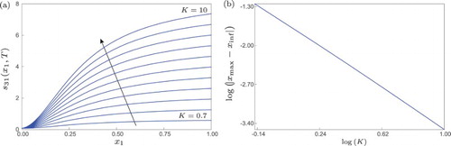
There are cases where an extremal point of the largest FTLE and the inflection point of a stimulus–response are exactly the same, see for instance Example 4.2. This can be explained in terms of Theorem 4.2, which gives an estimate for the modulus of the directional derivative of all FTLE. Therefore, the utilization of FTLE to identify activation thresholds has to be carried out with care, in view of the results shown in this paper. According to our study, all we can expect in general is that the extremal point of the largest FTLE and the inflection point of a stimulus–response curve lie in a certain interval $[\alpha ,\beta ]$, whose size will depend on how steep the stimulus–response curve is, see Theorem 4.1 and the remark thereafter. A closer look into this matter is given in the numerical experiment shown in Figure 4. In panel (a) we computed a family of sigmoidal stimulus–response curves of system (35(32) $\begin{array}{rl}{\eta }_j(x_j,T)& =\frac{1}{T}\ln \left({∥\mathrm{\Psi }(x_1,\dots ,x_j,\dots ,x_d,T)∥}_2\right)\\ & \le \frac{1}{T}\ln \left(d\underset{p,q=1,\dots ,d}{max}\left|\left(\mathrm{\Psi }\right(x_1,\dots ,x_j,\dots ,x_d,T){)}_{pq}\right|\right)\\ & \le \frac{1}{T}\ln \left(d\delta \right)\\ & <\frac{1}{T}\ln \left(M\right).\end{array}$(32) ) obtained by varying the parameter K. Here, we can see that the steepness of the stimulus–response curves increases as the parameter grows. Furthermore, we investigated how the difference between the inflection point $x_{\inf }$ of the stimulus–response curve $s_{31}(\cdot ,T)$ and the maximum point $x_{\max }$ of the induced FTLE ${\eta }_1(\cdot ,T)$ varies with respect to K. The result is shown in Figure 4(b) in logarithmic scale. The almost straight line indicates that the difference $\left|x_{\max }-x_{\inf }\right|$ decreases as fast as $\mathcal{O}\left(K^{-p}\right)$, with $p\approx 2$. Therefore, the numerical observations confirm the relation between steepness of stimulus–response curves and approximation of their inflection points by maximum points of FTLE, as predicted by Theorem 4.1.

Figure 4. (a) Sigmoidal stimulus–response curves of system (35(32) $\begin{array}{rl}{\eta }_j(x_j,T)& =\frac{1}{T}\ln \left({∥\mathrm{\Psi }(x_1,\dots ,x_j,\dots ,x_d,T)∥}_2\right)\\ & \le \frac{1}{T}\ln \left(d\underset{p,q=1,\dots ,d}{max}\left|\left(\mathrm{\Psi }\right(x_1,\dots ,x_j,\dots ,x_d,T){)}_{pq}\right|\right)\\ & \le \frac{1}{T}\ln \left(d\delta \right)\\ & <\frac{1}{T}\ln \left(M\right).\end{array}$(32) ) (with ${\eta }_{\mathrm{H}}=2$, ${\rho }_{\mathrm{H}}=1$) for T=2, $x_2=0.1$, $x_3=0.5$ and $0.7\le K\le 10$. The arrow indicates the direction of increasing K. (b) Difference between the inflection point $x_{\inf }$ of the stimulus–response curve $s_{31}(\cdot ,T)$ and the maximum point $x_{\max }$ of the induced FTLE ${\eta }_1(\cdot ,T)$, as a function of the parameter K.

Another aspect analysed numerically by Rateitschak and Wolkenhauer [19] is the detection of activation thresholds via extremal points of MCC. Their numerical observations indicate that MCC do not reliably detect all thresholds and suffer from false positives. In order to gain more insight into this matter, we tried to establish a relation between extremal points of MCC and inflection points of stimulus–response curves, and reached to the same conclusion, analytically shown in Equation (36(33) $\begin{array}{rl}\left|\frac{\mathrm{\partial }{\lambda }_k}{\mathrm{\partial }v}(x,T)\right|& \le \frac{1}{T{\mu }_k\left(\mathrm{\Psi }\right(x,T\left)\right)}{∥{\left(⟨\mathrm{\nabla }\frac{\mathrm{\partial }{P}_i}{\mathrm{\partial }{x}_j}(x,T),v⟩\right)}_{i,j=1,\dots ,d}∥}_2,\\ & x\in {\mathbb{R}}^d,T\in (0,T_0],k=1,\dots ,d,\end{array}$(33) ).

Acknowledgments

The authors would like to thank Dr K. Rateitschak for fruitful discussions.

Disclosure statement

No potential conflict of interest was reported by the authors.

Additional information

Funding

This work was partially supported by the German Science Foundation DFG [grant number Si801-6] and by the Vietnam National Foundation for Science and Technology Development (NAFOSTED) [grant number 101.03-2014.42]. The second author has been supported by a Georg Forster Research Fellowship granted by the Alexander von Humboldt Foundation, Germany. We acknowledge support by the German Research Foundation and the Open Access Publication Funds of the TU Dresden.

References

- B.B. Aldridge, G. Haller, P.K. Sorger, and D.A. Lauffenburger, Direct Lyapunov exponent analysis enables parametric study of transient signalling governing cell behaviour, Syst. Biol. 153(6) (2006), pp. 425–432. doi: 10.1049/ip-syb:20050065
- H.W. Bode, Network Analysis and Feedback Amplifier Design, D. Van Nostrand Co., Inc., New York, 1945.
- S. Choi (ed.), Introduction to Systems Biology, Humana Press, New Jersey, 2007.
- A. Goldbeter and D.E. Koshland, An amplified sensitivity arising from covalent modification in biological systems, Proc. Natl. Acad. Sci. USA 78(11) (1981), pp. 6840–6844. doi: 10.1073/pnas.78.11.6840
- G.H. Golub and C.F. Van Loan, Matrix Computations, 4th ed., The Johns Hopkins University Press, Baltimore, MD, 2013.
- S. Goutelle, M. Maurin, F. Rougier, X. Barbaut, L. Bourguignon, M. Ducher, and P. Maire, The Hill equation: A review of its capabilities in pharmacological modelling, Fund. Clin. Pharmacol. 22(6) (2008), pp. 633–648. doi: 10.1111/j.1472-8206.2008.00633.x
- G. Haller, Finding finite-time invariant manifolds in two-dimensional velocity fields, Chaos 10(1) (2000), pp. 99–108. doi: 10.1063/1.166479
- G. Haller, A variational theory of hyperbolic Lagrangian coherent structures, Phys. D 240(7) (2011), pp. 574–598. doi: 10.1016/j.physd.2010.11.010
- G. Haller and T. Sapsis, Lagrangian coherent structures and the smallest finite-time Lyapunov exponent, Chaos 21(2) (2011) (7 p.). doi: 10.1063/1.3579597
- R. Heinrich and T.A. Rapoport, Linear steady-state treatment of enzymatic chains. General properties, control and effector strength, Eur. J. Biochem. 42(1) (1974), pp. 89–95. doi: 10.1111/j.1432-1033.1974.tb03318.x
- R. Heinrich and S. Schuster, The Regulation of Cellular Systems, Chapman & Hall, New York, 1996.
- A.V. Hill, The possible effects of the aggregation of the molecules of haemoglobin on its dissociation curves, J. Physiol. 40 (1910), pp. 4–7.
- R.A. Horn and C.R. Johnson, Matrix Analysis, 2nd ed., Cambridge University Press, New York, 2013.
- B.P. Ingalls and H.M. Sauro, Sensitivity analysis of stoichiometric networks: An extension of metabolic control analysis to non-steady state trajectories, J. Theoret. Biol. 222(1) (2003), pp. 23–36. doi: 10.1016/S0022-5193(03)00011-0
- H. Kacser and J.A. Burns, The control of flux, Symp. Soc. Exp. Biol. 27 (1973), pp. 65–104.
- P. Lansky, O. Pokora, and J.-P. Rospars, Stimulus–Response Curves in Sensory Neurons: How to Find the Stimulus Measurable with the Highest Precision, Proceedings of the Second International Symposium on Brain, Vision and Artificial Intelligence, Naples, 2007, pp. 338–349.
- T. Millat, E. Bullinger, J. Rohwer, and O. Wolkenhauer, Approximations and their consequences for dynamic modelling of signal transduction pathways, Math. Biosci. 207(1) (2007), pp. 40–57. doi: 10.1016/j.mbs.2006.08.012
- M. Mohtashemi and R. Levins, Transient dynamics and early diagnostics in infectious disease, J. Math. Biol. 43(5) (2001), pp. 446–470. doi: 10.1007/s002850100103
- K. Rateitschak and O. Wolkenhauer, Thresholds in transient dynamics of signal transduction pathways, J. Theoret. Biol. 264(2) (2010), pp. 334–346. doi: 10.1016/j.jtbi.2010.02.001
- S.C. Shadden, F. Lekien, and J.E. Marsden, Definition and properties of Lagrangian coherent structures from finite-time Lyapunov exponents in two-dimensional aperiodic flows, Phys. D 212(3–4) (2005), pp. 271–304. doi: 10.1016/j.physd.2005.10.007
- A. Tiwari, J.C.J. Ray, J. Narula, and O.A. Igoshin, Bistable responses in bacterial genetic networks: Designs and dynamical consequences, Math. Biosci. 231(1) (2011), pp. 76–89. doi: 10.1016/j.mbs.2011.03.004