
 ?Mathematical formulae have been encoded as MathML and are displayed in this HTML version using MathJax in order to improve their display. Uncheck the box to turn MathJax off. This feature requires Javascript. Click on a formula to zoom.
ABSTRACT
Based on previous research, we formulate revised, new, simple models for interactive wild and sterile mosquitoes which are better approximations to real biological situations but mathematically more tractable. We give basic investigations of the dynamical features of these simple models such as the existence of equilibria and their stability. Numerical examples to demonstrate our findings and brief discussions are also provided.
1. Introduction
Mosquito-borne diseases, such as malaria and dengue fever, are considerable public health concerns worldwide. These diseases are transmitted between humans by blood-feeding mosquitoes. No vaccines are available and an effective way to prevent these mosquito-borne diseases is to control mosquitoes. Among the mosquitoes control measures, the sterile insect technique (SIT) has been applied to reducing or eradicating wild mosquitoes. The SIT is a method of biological control in which the natural reproductive process of mosquitoes is disrupted. Utilizing radical or other chemical or physical methods, male mosquitoes are genetically modified to be sterile which are incapable of producing offspring despite being sexually active. These sterile mosquitoes are then released into the environment to mate with wild mosquitoes that are present in the environment. A wild female that mates with a sterile male will either not reproduce, or produce eggs but the eggs will not hatch. Repeated releases of sterile mosquitoes or releasing a significantly large number of sterile mosquitoes may eventually wipe out or control a wild mosquito population [Citation1,Citation7,Citation21].
Mathematical models have been formulated in the literature to study the interactive dynamics and control of the wild and sterile mosquito populations [Citation2–6,Citation11,Citation12]. In particular, models incorporating different strategies in releasing sterile mosquitoes have been formulated and studied in [Citation9,Citation16]. The wild and sterile mosquitoes are assumed homogeneous in these models which makes the model reasonably simple and the analysis tractable. Nevertheless, since mosquitoes undergo complete metamorphosis going through four distinct stages of development during a lifetime: egg, pupa, larva, and adult [Citation8], simple stage-structured models are formulated in [Citation17] where the wild mosquitoes are divided into two groups one of which is composed of the three aquatic stages. While interspecific competition and predation may cause larval mortality, intraspecific competition could represent a major density dependent source for the population dynamics, and hence the effect of crowding could be an important factor in the population dynamics of mosquitoes [Citation10,Citation13,Citation18]. Density dependence then is included in both the homogeneous and stage-structured models in [Citation9,Citation16,Citation17] to make all model systems nonlinear.
Comparing the homogeneous and stage-structured models, the model formulations in [Citation17] are more reasonable and realistic. However, since our goal is, after having a fundamental understanding of the dynamics for the interactive mosquitoes, to have the mosquito models incorporated into disease transmission models for the mosquito-borne diseases [Citation14,Citation15], the three dimensional models for the mosquitoes make the analysis mathematically more difficult.
We also notice that the crowding basically takes place in water where the egg, pupa, and larva stages in a mosquito's life cycle present. That is, the mosquito population density dependence mostly exists in the first three aquatic stages. Thus, the density dependence for the sterile mosquitoes, which are basically adult mosquitoes, can be ignored, and the density dependence for the wild mosquitoes need to be focused on the newborns survivals.
Based on the better understanding we obtained from the model analysis in [Citation17], we revise the models studied in [Citation9] and formulate new simple models in this paper. To make the models as simple as possible, we still assume homogeneous populations such that no stage distinction is concerned. We focus the density dependence on the larvae development process and assume the death rates for wild and sterile mosquitoes are density independent [Citation19,Citation20,Citation22]. We first give general modelling descriptions in Section 2. We then consider three strategies of releases, similar to those in [Citation9,Citation17] to formulate different models, and give complete mathematical analyses for the model dynamics in Sections 3, 4, and 5, respectively. Numerical examples are provided as well to confirm our analytic results, and we finally give brief discussions on our findings in Section 6.
2. Model formulation
Based on the works in [Citation2–6], homogeneous models for the interactive wild and sterile mosquitoes were formulated in [Citation9]. Let be the number of wild mosquitoes and
the number of sterile mosquitoes at time t. Density dependence is assumed for the death rates of both wild and sterile mosquitoes. The model, in a more general setting, has the form
(1)
(1) where
is the number of matings per individual, per unit of time, with N=w + g; a is the number of wild offspring produced per mate;
and
, i=1,2, are the density independent and dependent death rates of the wild and sterile mosquitoes, respectively, and
is the release rate of the sterile mosquitoes. With different mating rates, possible Allee effects, and three strategies of releases, fundamental analysis was carried out and results were obtained. System (Equation1
(1)
(1) ) is based on the classical Lotka–Volterra model. The populations are homogeneous and density dependence is assumed in both the wild and sterile mosquitoes death rates.
Considering the distinct metamorphic stages of mosquitoes, stage-structured models were formulated and studied in [Citation17]. The three aquatic stages of wild mosquitoes were grouped into one class, called the larvae class and denoted by J, and adult stage was kept as a separate class and denoted by A in the models. Introducing the number of sterile mosquitoes at time t, denoted by , into the two classes of wild mosquitoes, an interactive model, in more general setting, was described by the following system
(2)
(2) where σ is the number of offspring produced per wild mosquito through all matings, per unit of time,
is the density independent death rate and
is the density dependent death factor for larvae,
, i=1,2, are the adults death rates which are assumed density independent. Based on three strategies of releases, fundamental investigations were performed. Stage structure is included in the model. Note that the sterile mosquitoes released are adult mosquitoes and the competition between adult mosquitoes are relatively weak. Moreover, while the intraspecific competition, or the effect of crowding, represents a major density dependent source in the population dynamics, the crowding basically takes place in water. The death rates for adult wild mosquitoes and sterile mosquitoes are then assumed density independent.
Each of the two models has its strong as well as weak points. In the mean time, from the relatively full investigations, it was shown that the dynamic features of the two models (Equation1(1)
(1) ) and (Equation2
(2)
(2) ) are similar. As mentioned in Section 1, our goal is, after gaining a better understanding of the interactive dynamics of the wild and sterile mosquitoes, to have the mosquitoes models incorporated into the transmission models of diseases. Thus, it is beneficial and even necessary in practice to keep the mosquitoes models as simple as possible, but more accurate and realistic. To this end, learning from the strong points of the two models in systems (Equation1
(1)
(1) ) and (Equation2
(2)
(2) ), we propose in this paper new revised models for the interactive wild and sterile mosquitoes. We keep using the two dimensional homogeneous models based on system (Equation1
(1)
(1) ) but assume that the density dependence only affects the survivals of the larvae and hence appears only in the birth term of the wild mosquitoes.
Let be the number of wild mosquitoes at time t. In the absence of sterile mosquitoes, the dynamics of
are governed by
(3)
(3) where
is the birth function, and constant
is the death rate of the wild mosquitoes.
We assume that the birth function has the form
where
is the mating rate, a is the maximum number of survived offspring reproduced per individual, and
is the carrying capacity parameter such that
describes the density dependent survival probability.
If the mating rate is constant, written as , Equation (Equation3
(3)
(3) ) becomes the classical logistic equation
Considering the possible difficult for mosquitoes to find their mates when the population size of mosquitoes is small, we assume an Allee effect such that the mating rate takes a form of Holling-II type with . Then Equation (Equation3
(3)
(3) ) becomes
(4)
(4) where we merge c and a but still denote it as a.
Clearly, the trivial equilibrium is a locally asymptotically stable equilibrium for
Equation (Equation4
(4)
(4) ). Set the right-hand side of Equation (Equation4
(4)
(4) ) equal to zero. A positive equilibrium of system (Equation4
(4)
(4) ) satisfies
where
(5)
(5) with
, the intrinsic growth rate of wild mosquitoes in the absence of sterile mosquitoes.
Function has real roots
(6)
(6) provided
. Thus, there exists no, one, or two positive equilibria of Equation (Equation4
(4)
(4) ) if
,
, or
, respectively.
Suppose such that there exist two positive equilibria. It follows from Equations (Equation4
(4)
(4) ) – (Equation6
(6)
(6) ) that, at a positive equilibrium,
Thus
and then positive equilibrium
is unstable, and
is asymptotically stable.
After sterile mosquitoes are released into the wild mosquito population, we let be the number of sterile mosquitoes at time t, and assume that the interactive birth rate of wild mosquitoes follows the harmonic mean. Then, if there is no Allee effect included, the birth function has the form
and the interactive dynamics are governed by the following system
(7)
(7) If an Allee effect is considered, we then have the following system
(8)
(8)
3. Constant releases
In this section, we suppose that the sterile mosquitoes are constantly released such that , a constant. Then no mating difficulty will be concerned and based on system (Equation7
(7)
(7) ), we have
(9)
(9)
Define set as
where we assume
. Then
is a positive invariant set for system (Equation9
(9)
(9) ). We assume
in this section.
System (Equation9(9)
(9) ) has a boundary equilibrium
, where
.
A positive equilibrium of system (Equation9(9)
(9) ) satisfies
where
(10)
(10) which has two solutions
(11)
(11) Define a threshold value of releases for system (Equation9
(9)
(9) ) by
(12)
(12) Then there exist no, one, or two positive solutions given in (Equation11
(11)
(11) ) to
in
Equation (Equation10
(10)
(10) ), that is, no, one, or two positive equilibria of system (Equation9
(9)
(9) ), if
,
, or
, respectively.
We next investigate the stability of the equilibria. The Jacobian matrix at an equilibrium has the form
where
at the boundary equilibrium. Thus the boundary equilibrium
is always asymptotically stable. Furthermore, if there exists no positive interior equilibrium, since set
is positively invariant, according to the Poincaré-Bendixson Theorem,
is globally asymptotically stable.
At a positive equilibrium,
and thus, in addition to following from Equation (Equation10
(10)
(10) ),
Then, at positive equilibria and
,
and
which implies that
is a saddle point and
is a locally asymptotically stable node. In summary, we have
Theorem 3.1:
Assume . System (Equation9
(9)
(9) ) has a boundary equilibrium
with
which is globally asymptotically stable if there exists no positive equilibrium, and locally asymptotically stable if a positive equilibrium exists. System (Equation9
(9)
(9) ) has no, one, or two positive equilibria if
or
respectively, where the release threshold
is given in (Equation12
(12)
(12) ). If there exist two positive equilibria,
and
where
are given in (Equation11
(11)
(11) ),
is an unstable saddle point and
is a locally asymptotically stable node.
We give an example to illustrate the results in Theorem 3.1 as follows.
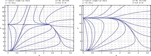
Example 1:
Parameters are given as
(13)
(13) and thus the release threshold is
.
Boundary equilibrium is asymptotically stable. With
, there exist two positive equilibria
and
. Equilibrium
is a saddle point and
is a locally asymptotically stable node. Solutions approach either
or
depending on their initial values, as shown in the left side of Figure . For
, there exists no positive equilibrium and
is globally asymptotically stable. All solutions approach
as shown in the right side of Figure .
Figure 1. Parameters are given in (Equation13(13)
(13) ) and the release threshold is
. For
, there are two positive equilibria
and
. Equilibrium
is a saddle point and
is a locally asymptotically stable node, solutions approach
or the locally asymptotically stable boundary equilibrium
depending on their initial values, as shown in the left-side figure. For
, no positive equilibrium exists and
becomes globally asymptotically stable. All solutions approach
as shown in the right-side figure.
4. Releases proportional to the wild mosquitoes
As in [Citation9,Citation17], to have a more optimal and economically effective strategy of releasing sterile mosquitoes in an area where the population size of wild mosquitoes is relatively small, we may consider to keep closely sampling or surveillance of the wild mosquito population and let the rate of releases be proportional to the population size of the wild mosquitoes such that where b is a constant. In the meantime, in a situation where a small mosquito population size may cause possible mating difficulty, we assume an Allee effect and thus the interactive system for the wild and sterile mosquitoes, based on system (Equation8
(8)
(8) ), has the form
(14)
(14)
Define set as
where
is given in (Equation6
(6)
(6) ). Then
is a positive invariant set for system (Equation14
(14)
(14) ). We assume
in this section.
The origin is a trivial equilibrium and is always locally asymptotical stable. A positive equilibrium of system (Equation14
(14)
(14) ) satisfies the following equation
where
(15)
(15) which has two roots
(16)
(16) If
, then there are no positive roots to
, that is, no positive equilibria to system (Equation14
(14)
(14) ).
Assume . Then
, if and only if
. Define the threshold value of releases as
(17)
(17) Then system (4) has no, one, or two positive equilibria of system (Equation9
(9)
(9) ) if
,
, or
, respectively.
Assume so that there exist two positive equilibria, denoted by
and
. We investigate the stability of the positive equilibria as follows.
The Jacobian matrix at an equilibrium has the form
where
Thus, writing
we have
(18)
(18) It follows from Equation (Equation15
(15)
(15) ) that, at an equilibrium,
Substituting it into Equation (Equation18
(18)
(18) ) yields
(19)
(19) Then substituting (Equation16
(16)
(16) ) into Equation (Equation19
(19)
(19) ), we have
Notice that
Then
and thus we have the determinant of the Jacobian at
,
.
At , writing
we have
which implies that the determinant of
at
has
. Hence
is an unstable saddle point.
Moreover, at ,
where
(20)
(20) It follows from Equation (Equation15
(15)
(15) ) that
Substituting it into Equation (Equation20
(20)
(20) ) then yields
Thus
and hence positive equilibrium
is a locally asymptotically stable node or spiral.
In summary, we have the following results.
Theorem 4.1:
The origin is a trivial equilibrium of system (Equation14
(14)
(14) ), which is always locally asymptotically stable. Assume
. Then system (Equation14
(14)
(14) ) has no, one, or two positive equilibria if
or
respectively, where the release threshold
is given in (Equation17
(17)
(17) ). If there exist two positive equilibria,
and
where
are given in (Equation16
(16)
(16) ), equilibrium
is an unstable saddle point and
is a locally asymptotically stable node or spiral.
A numerical example for the proportional releases of sterile mosquitoes is given below.
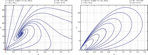
Example 2:
With the same parameters as in Example 1, that is,
(21)
(21) the release threshold is
.
When , there exist two positive equilibria
and
. Equilibrium
is a saddle point and
is a locally asymptotically spiral. Solutions approach either
or the origin depending on their initial values as shown in the left side of Figure . For
, there exists no positive equilibrium and the origin is globally asymptotically stable. All solutions approach the origin as shown in the right side of Figure .
Figure 2. Parameters are given in (Equation21(21)
(21) ) and the release threshold is
. For
, there are two positive equilibria
and
. Equilibrium
is a saddle point and
is a locally asymptotically spiral. Solutions approach either
or the origin depending on their initial values as shown in the left-side figure. For
, there exists no positive equilibrium. The origin is globally asymptotically stable. All solutions approach the origin as shown in the right-side figure.
5. Proportional releases with saturation
A new strategy to compromise the two strategies studied in Sections 3 and 4 was proposed in [Citation9,Citation17], where the release rate is proportional to as
small, but is saturated and approaches a constant as
sufficiently large. Let
, and the interactive dynamics of the wild and sterile mosquitoes are governed by the following system
(22)
(22)
Define set as
where
is given in (Equation6
(6)
(6) ). Then
is a positive invariant set for system (Equation22
(22)
(22) ). We assume
in this section.
The origin is a trivial equilibrium and is always locally asymptotical stable. A positive equilibrium of system (Equation22
(22)
(22) ) satisfies the following equation
where
Clearly, the positive equilibria of (Equation22
(22)
(22) ) correspond to the positive roots of
. Since there exist at most two positive roots of
, there exist at most two positive equilibria of (Equation22
(22)
(22) ).
Rewrite
where
is given in (Equation5
(5)
(5) ). For fixed parameters, if there is no positive root for
, that is, no intersection between the curve of
and the positive
-axis, the curve of
has no intersection with the positive
-axis for
. Hence there is no positive equilibrium of system (Equation22
(22)
(22) ) if
.
Suppose . The curve of
for b=0, that is the curve of
, intersects the positive
-axis twice. It is clear that the curve of
moves up as b increases and is completely above the positive
-axis as b sufficiently large. Hence, there exists a threshold value of b, denoted by
, such that the curve is tangent to the positive
-axis, for all of other parameters fixed. Thus system (Equation22
(22)
(22) ) has no, one, or two, positive equilibria, if
,
, or
, respectively. Indeed, the threshold value
can be determined as follows.
At a positive critical point , the following two equations are satisfied simultaneously:
(23)
(23) which results in a unique
satisfying
(24)
(24) and then
(25)
(25)
We next work on the stability of the positive equilibria.
The Jacobian matrix at an equilibrium has the form
where
and
It follows from Equations (Equation23(23)
(23) ) that, at a positive equilibrium,
(26)
(26) Since
then Equation (Equation26
(26)
(26) ) leads to
Thus
(27)
(27) and
We then have
(28)
(28)
On the other hand, it follows from Equations (Equation23(23)
(23) ) and (Equation26
(26)
(26) ) that
Then
and thus
Hence, we have
and it follows from Equation (Equation27
(27)
(27) ) that
(29)
(29)
Suppose there exist two positive equilibria and
with
. Then
which implies, from Equation (Equation29
(29)
(29) ) that
Thus,
is an unstable saddle.
Moreover, we have, from Equation (Equation28(28)
(28) ),
Therefore, positive equilibrium
is a locally asymptotically stable node or saddle.
In summary, we have
Theorem 5.1:
The origin is a trivial equilibrium of system (Equation22
(22)
(22) ), which is always locally asymptotically stable. If
system (Equation22
(22)
(22) ) has no positive equilibrium. If
there exists a threshold value
given in (Equation25
(25)
(25) ) with
being the unique positive solution to Equation (24). System (Equation22
(22)
(22) ) has no, one, or two positive equilibria if
or
respectively. If there exist two positive equilibria
and
with
equilibrium
is an unstable saddle and
is a locally asymptotically stable node or spiral.
We give a numerical example for system (Equation22(22)
(22) ) as follows.
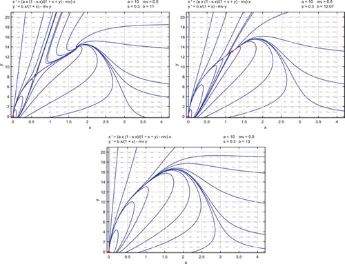
Example 3:
Given the parameters
(30)
(30) the solution
to system (Equation23
(23)
(23) ) is
and then
in (Equation25
(25)
(25) ).
With , there exist two positive equilibria
and
, in addition to the trivial equilibrium
which is a locally asymptotically stable node. Equilibrium
is a saddle point while
is a locally asymptotically stable spiral, as shown in the upper left side of Figure . As b increases but is less than
, the two positive equilibria move closer. For b=12.07,
is still a saddle point,
becomes a locally asymptotically stable node as shown in the upper right side of Figure . There is an unstable saddle-node point as
, and as
, there exists no positive equilibrium and all solutions approach the origin as shown in the lower part of Figure .
Figure 3. Parameters are given in (Equation30(30)
(30) ) and the release threshold is
. For
, there are two positive equilibria, one of which is a saddle point and one of which is a locally asymptotically stable spiral, as shown in the upper left-side figure. For b=12.07, the two positive equilibria move closer, where one is still saddle point and the other becomes a locally asymptotically stable node as shown in the upper right-side figure. For
, there exists no positive equilibrium and all solutions approach the origin as shown in the lower figure.
6. Concluding remarks
Based on the models in [Citation9,Citation17], we revised and formulated new simple models for the interactive wild and sterile mosquitoes in this paper. The main goal is to make the models more appropriately describing the biological situations, and in the meantime mathematically more tractable.
While mosquitoes undergo complete metamorphosis going through distinct stages of development during a lifetime, and hence stage-structured models are needed, the investigations on the stage-structured models in [Citation17] and the simplified homogeneous models without stage structure in [Citation9] showed that they exhibited very similar dynamical features. Since our fundamental goal of these studies is to eventually have the interactive mosquitoes models incorporated into transmission models of mosquito-borne diseases in higher dimensional spaces, a reduction of even one dimension in the model formulation could benefit our further research. Hence, it seems reasonable to keep using two-dimensional homogeneous models for the interaction of wild and sterile mosquitoes but with modifications.
We note that the released sterile mosquitoes are all adults. The competition for resources between the adult mosquitoes are relatively weak and as a result, it seems reasonable to assume density independent death rates for both wild and sterile mosquitoes. In the meantime, the intraspecific competition could represent a major density dependent source for the larvae development, and in particular, the crowding basically takes place in water. Thus, we need to have the density dependence more focused on the birth terms, more specifically, on the survivals of the newborns. Comparing to the models in [Citation9], we thus assume that the birth rate has the form of with a the maximum reproduction rate. With such revisions, we believe that the models are more biologically appropriate and better fitting our research design.
We fully studied the dynamical features for the models formulated in this paper. We determined the existence of all possible equilibria and completely investigated their stability for the three models with different strategies of releases in Sections 3,4, and 5. We established release threshold values of sterile mosquitoes for each model. As the release rate of sterile mosquitoes exceeds the threshold value, there exists no positive equilibrium, and the boundary equilibrium for the constant releases and the trivial equilibrium for the other two strategies are globally asymptotically stable, which means all wild mosquitoes go extinct eventually. On the other hand, it the release rate is less than the threshold value, all of the three models have two positive interior equilibria one of which is always a saddle point, and one of which is locally asymptotically stable. The stable equilibrium for the constant releases is a node, but it can be either a node or a spiral for the other strategies of releases. This is different from the model dynamics in [Citation9,Citation17].
The model dynamics are relatively simple compared to the models in [Citation9,Citation17], but again since the focus of modelling mosquitoes interactions is on our fundamental goal of having the mosquito models incorporated into disease transmission models, this is exactly what we need. Further studies on the impact of releases of sterile mosquitoes on disease transmissions, based on the interactive mosquito models in this paper, will benefit from such revisions, and will appear in the near future. We would also like to point out that the new models in this paper can be applied to other interacting species as well.
Acknowledgments
The author thanks the handling editor and two anonymous reviewers for their valuable comments and suggestions.
Disclosure statement
No potential conflict of interest was reported by the authors.
Additional information
Funding
References
- L. Alphey, M. Benedict, R. Bellini, G.G. Clark, D.A. Dame, M.W. Service, and S.L. Dobson, Sterile-insect methods for control of mosquito-borne diseases: An analysis, Vector Borne Zoonotic Dis. 10 (2010), pp. 295–311. doi: 10.1089/vbz.2009.0014
- H.J. Barclay, The sterile insect release method on species with two-stage life cycles, Res. Popul. Ecol. 21 (1980), pp. 165–180. doi: 10.1007/BF02513619
- H.J. Barclay, Pest population stability under sterile releases, Res. Popul. Ecol. 24 (1982), pp. 405–416. doi: 10.1007/BF02515585
- H.J. Barclay, Modeling incomplete sterility in a sterile release program: Interactions with other factors, Popul. Ecol. 43 (2001), pp. 197–206. doi: 10.1007/s10144-001-8183-7
- H.J. Barclay, Mathematical models for the use of sterile insects, in Sterile Insect Technique. Principles and Practice in Area-Wide Integrated Pest Management, V.A. Dyck, J. Hendrichs, and A.S. Robinson eds., Springer, Heidelberg, 2005, pp. 147–174.
- H.J. Barclay and M. Mackauer, The sterile insect release method for pest control: A density dependent model, Environ. Entomol. 9 (1980), pp. 810–817. doi: 10.1093/ee/9.6.810
- A.C. Bartlett and R.T. Staten, Sterile Insect Release Method and other Genetic Control Strategies, Radcliffe's IPM World Textbook, 1996. Available at https://protect-us.mimecast.com/s/zNXlBdUbR4D5cD?domain=ipmworld.umn.edu.
- N. Becker, Mosquitoes and Their Control, Kluwer Academic/Plenum, New York, 2003.
- L. Cai, S. Ai, and J. Li, Dynamics of mosquitoes populations with different strategies for releasing sterile mosquitoes, SIAM J. Appl. Math. 74 (2014), pp. 1786–1809. doi: 10.1137/13094102X
- C. Dye, Intraspecific competition amongst larval Aedes aegypti: Food exploitation or chemical interference, Ecol. Entomol. 7 (1982), pp. 39–46. doi: 10.1111/j.1365-2311.1982.tb00642.x
- K.R. Fister, M.L. McCarthy, S.F. Oppenheimer, and C. Collins, Optimal control of insects through sterile insect release and habitat modification, Math. Biosci. 244 (2013), pp. 201–212. doi: 10.1016/j.mbs.2013.05.008
- J.C. Flores, A mathematical model for wild and sterile species in competition: Immigration, Phys. A 328 (2003), pp. 214–224. doi: 10.1016/S0378-4371(03)00545-4
- R.M. Gleiser, J. Urrutia, and D.E. Gorla, Effects of crowding on populations of Aedes albifasciatus larvae under laboratory conditions, Entomol. Exp. Appl. 95 (2000), pp. 135–140. doi: 10.1046/j.1570-7458.2000.00651.x
- J. Li, Malaria model with stage-structured mosquitoes, Math. Biol. Eng. 8 (2011), pp. 753–768. doi: 10.3934/mbe.2011.8.753
- J. Li, Modeling of transgenic mosquitoes and impact on malaria transmission, J. Biol. Dynam. 5 (2011), pp. 474–494. doi: 10.1080/17513758.2010.523122
- J. Li and Z. Yuan, Modeling releases of sterile mosquitoes with different strategies, J. Biol. Dynam. 9 (2015), pp. 1–14. doi: 10.1080/17513758.2014.977971
- J. Li, L. Cai, and Y. Li, Stage-structured wild and sterile mosquito population models and their dynamics, J. Biol. Dynam. (2016). Available at https://protect-us.mimecast.com/s/rx4mBRUMbaWRTa?domain=dx.doi.org.
- M. Otero, H.G. Solari, and N. Schweigmann, A stochastic population dynamics model for Aedes aegypti: Formulation and application to a city with temperate climate, Bull. Math. Biol. 68 (2006), pp. 1945–1974. doi: 10.1007/s11538-006-9067-y
- C.M. Stone, Transient population dynamics of mosquitoes during sterile male releases: Modelling mating behaviour and perturbations of life history parameters, PLoS ONE 8 (2013), p. e76228. doi: 10.1371/journal.pone.0076228
- S.M. White, P. Rohani, and S.M. Sait, Modelling pulsed releases for sterile insect techniques: Fitness costs of sterile and transgenic males and the effects on mosquito dynamics, J. Appl. Ecol. 47 (2010), pp. 1329–1339. doi: 10.1111/j.1365-2664.2010.01880.x
- Wikipedia, Sterile insect technique, 2014. Available at https://protect-us.mimecast.com/s/ZpWJBRu1q48kTn?domain=en.wikipedia.org.
- L. Yakob, L. Alphey, and M.B. Bonsall, Aedes aegypti control: The concomitant role of competition, space and transgenic technologies, J. Appl. Ecol. 45 (2008), pp. 1258–1265. doi: 10.1111/j.1365-2664.2008.01498.x