Optimal control of the Lotka–Volterra system: turnpike property and numerical simulations

ABSTRACT

The Lotka–Volterra model is a differential system of two coupled equations representing the interaction of two species: a prey one and a predator one. We formulate an optimal control problem adding the effect of hunting both species as the control variable. We analyse the optimal hunting problem paying special attention to the nature of the optimal state and control trajectories in long time intervals. To do that, we apply recent theoretical results on the frame to show that, when the time horizon is large enough, optimal strategies are nearly steady-state. Such path is known as turnpike property. Some experiments are performed to observe such turnpike phenomenon in the hunting problem. Based on the turnpike property, we implement a variant of the single shooting method to solve the previous optimisation problem, taking the middle of the time interval as starting point.

KEYWORDS:

• Lotka–Volterra
• optimal control
• turnpike
• indirect shooting method

AMS SUBJECT CLASSIFICATION:

• 49J15
• 78A70
• 34K28

1. Introduction

The Turnpike property is a general phenomenon which holds for a large class of optimal control problems. Roughly speaking, the turnpike property allows approximating the solution of the optimal control problem through the solution of the static problem.

In this work, in the frame of the optimal control theory, we apply one of the most recent results on the Turnpike phenomenon to a classical and relevant biological model: the controlled Lotka–Volterra ODE system with two interacting populations. Even if no theoretical novelty is presented, we show how the turnpike phenomenon can be used to improve numerical methods for solving optimal control problems. We give a detailed description of the new algorithm and perform some simulations to show the numerical efficiency.

The major contribution of our work is that we show the striking efficiency obtained from the combination of the turnpike with a classic numerical method. We would like to focus on the theoretical and numerical significance of the application of the turnpike theory in an applied biological case. It is theoretically important as it gives information about the solution of the optimal control problem without the need of solving it. Its numerical importance is weighed by its application to improve the numerical methods.

The optimal control theory has been successfully applied to a wide range of real problems such as in neurology, to explain the behaviour of the sensorimotor system using a feedback optimal control law [29,30,32,33]. It can also be used to determine the best way to administer different drugs and treatments to deal with a cancerous tumour [16,17,31], or getting the optimal vaccination protocol to face an epidemic [15,18].

Dynamic population models are also a rich area in which optimal control theory can be applied. For example, it can be used to design a control for invasive species minimising the cost of the control and the damage [20], or to find the best way to augment certain declining populations [3].

The Lotka–Volterra equations, also known as predator–prey equations, were developed independently by Lotka [19] and Volterra [37] in 1926. It models biological systems where two species interact: a prey and a predator. The evolution of the species is given by the following system: (1) $\frac{\mathrm{d}{x}_1\left(t\right)}{\mathrm{d}t}=x_1\left(t\right)(\alpha -\beta x_2(t\left)\right),$(1) (2) $\frac{\mathrm{d}{x}_2\left(t\right)}{\mathrm{d}t}=-x_2\left(t\right)(\gamma -\delta x_1(t\left)\right),$(2) (3) $x_1\left(0\right)=x_1^0,x_2\left(0\right)=x_2^0,$(3) where $x_1\left(t\right)$ and $x_2\left(t\right)$ represent the prey and predator populations, respectively, and $\alpha ,\beta ,\gamma$ and δ are real positive constant parameters characterising each species. This model is the first to represent the interaction of more than one species (Figure 1).

Figure 1. (a) Solution of Equation (3(3) $x_1\left(0\right)=x_1^0,x_2\left(0\right)=x_2^0,$(3) ) for the initial condition $x_1\left(0\right)=0.5,x_2\left(0\right)=0.7$ in the time interval $[0,60]$ (b): Orbits for positive initial conditions $(1/2,1/2)$, $(1/4,1/4)$ and $(1/8,1/8)$.

The Lotka–Volterra model assumes that the food supply for the prey is unlimited and the rate of change of population is proportional to its size. Without a predator, the prey species grows exponentially, while the predator has a constant per capita death rate. Besides that, the presence of the prey increases the predator population, while the presence of the predator species reduces the prey population [4].

Originally, Volterra developed this model to describe the evolution of the fish population of the Adriatic Sea. Of course, it can be used to explain many other predator–prey interactions where the food source of the prey is almost unlimited, like wolves and goats. But the applications of the Lotka–Volterra model goes beyond animal interactions. In the work of Lotka [19], this model was developed to describe certain chemical reactions applying the chemical law for mass action. In epidemiology, the Lotka–Volterra system has been used to model the evolution of certain microorganisms, such as the experiments Gause made in 1934 [4]. In this work, we will try to study the most general case, in which many different applications could be included.

An interesting question is how can we influence it, i.e. if by choosing a good mechanism we are able to lead the system from an initial state $(x_1^0,x_2^0)$ to a certain prefixed objective, or a desired final state $(x_1^f,x_2^f)$ in time T. Shortly, we can consider it as a control problem. In this work, hunting is considered the control of system (3(3) $x_1\left(0\right)=x_1^0,x_2\left(0\right)=x_2^0,$(3) ).

A general formulation of a control system for the predator–prey model (3(3) $x_1\left(0\right)=x_1^0,x_2\left(0\right)=x_2^0,$(3) ) is as follows: (4) $\frac{\mathrm{d}{x}_1\left(t\right)}{\mathrm{d}t}=x_1\left(t\right)(\alpha -\beta x_2(t\left)\right)-x_1\left(t\right)c_1{u}_{[0,1]}\left(t\right),$(4) (5) $\frac{\mathrm{d}{x}_2\left(t\right)}{\mathrm{d}t}=-x_2\left(t\right)(\gamma -\delta x_1(t\left)\right)-x_2\left(t\right)c_2{u}_{[0,1]}\left(t\right),$(5) (6) $\left(x_1\right(0),x_2(0\left)\right)=(x_1^0,x_2^0),$(6) where $u_{[0,1]}\in L^2(0,T;[0,1\left]\right)$ (i.e. $u_{[0,1]}\left(t\right)\in [0,1]$), is the constrained control parameter representing the amount of individuals of each population that is removed from the sea at time t. The constants $c_1,c_2$ represent the maximum level of hunting in a time instant t for each population ($c_1=1$ means that there is no fishing limit).

It is remarked that the formulation of problem (4(2) $\frac{\mathrm{d}{x}_2\left(t\right)}{\mathrm{d}t}=-x_2\left(t\right)(\gamma -\delta x_1(t\left)\right),$(2) )–(6(6) $\left(x_1\right(0),x_2(0\left)\right)=(x_1^0,x_2^0),$(6) ) is very general and it can be applied to many specific cases.

Problem (4(2) $\frac{\mathrm{d}{x}_2\left(t\right)}{\mathrm{d}t}=-x_2\left(t\right)(\gamma -\delta x_1(t\left)\right),$(2) )–(6(6) $\left(x_1\right(0),x_2(0\left)\right)=(x_1^0,x_2^0),$(6) ) can be treated as an optimization problem. Let define a cost function $C_T\left(u\right)$ representing the objective, and let try to find the control minimising such cost function in time T, under certain restrictions.

We can find different ways to apply the optimal control theory to the Lotka–Volterra model [2,8,27,40]. Let us consider the following cost function: (7) $C_T\left(u_{[0,1]}\right)=\frac{1}{2}{\int }_0^{\mathrm{T}}\left(\right(x_1\left(t\right)-a{)}^2+\left(x_2\right(t)-b{)}^2+(u_{[0,1]}\left(t\right)-c{)}^2)\mathrm{d}t.$(7)

To illustrate the turnpike phenomenon in this work, we are going to study the following large time optimal control problem in $L^2(0,T)$ (the coefficients α, β, γ, δ, $c_1$ and $c_2$ of system (7(7) $C_T\left(u_{[0,1]}\right)=\frac{1}{2}{\int }_0^{\mathrm{T}}\left(\right(x_1\left(t\right)-a{)}^2+\left(x_2\right(t)-b{)}^2+(u_{[0,1]}\left(t\right)-c{)}^2)\mathrm{d}t.$(7) ) have been chosen like in [27]): (8) $\frac{\mathrm{d}{x}_1\left(t\right)}{\mathrm{d}t}=x_1\left(t\right)-x_1\left(t\right)x_2\left(t\right)-0.4x_1\left(t\right)u_{[0,1]}\left(t\right),$(8) (9) $\frac{\mathrm{d}{x}_2\left(t\right)}{\mathrm{d}t}=-x_2\left(t\right)+x_1\left(t\right)x_2\left(t\right)-0.2x_2\left(t\right)u_{[0,1]}\left(t\right),$(9) (10) $\left(x_1\right(0),x_2(0\left)\right)=(0.5;0.7),$(10) (11) $T=60$(11) with the following cost function to minimize: (12) $\underset{u_{[0,1]}\in L^2(0,T;[0,1\left]\right)}{min}\frac{1}{2}{\int }_0^{\mathrm{T}}\left(\right(x_1\left(t\right)-1{)}^2+x_2(t{)}^2+u_{[0,1]}(t{)}^2)\mathrm{d}t.$(12)

See [13] for proofs of the existence of solutions of Equation (8(3) $x_1\left(0\right)=x_1^0,x_2\left(0\right)=x_2^0,$(3) )–(11(11) $T=60$(11) ) and the existence of a minimum of Equation (12(12) $\underset{u_{[0,1]}\in L^2(0,T;[0,1\left]\right)}{min}\frac{1}{2}{\int }_0^{\mathrm{T}}\left(\right(x_1\left(t\right)-1{)}^2+x_2(t{)}^2+u_{[0,1]}(t{)}^2)\mathrm{d}t.$(12) ).

Our interest is to study and numerically solve the Lotka–Volterra optimal control problem (8(3) $x_1\left(0\right)=x_1^0,x_2\left(0\right)=x_2^0,$(3) )–(11(11) $T=60$(11) ) with the cost functional (12(12) $\underset{u_{[0,1]}\in L^2(0,T;[0,1\left]\right)}{min}\frac{1}{2}{\int }_0^{\mathrm{T}}\left(\right(x_1\left(t\right)-1{)}^2+x_2(t{)}^2+u_{[0,1]}(t{)}^2)\mathrm{d}t.$(12) ) in long time intervals. To do that, we apply the theory proved in one of the most recent works about the turnpike theory [36] to the optimal control problem (8(3) $x_1\left(0\right)=x_1^0,x_2\left(0\right)=x_2^0,$(3) )–(11(11) $T=60$(11) ) with the cost functional (12(12) $\underset{u_{[0,1]}\in L^2(0,T;[0,1\left]\right)}{min}\frac{1}{2}{\int }_0^{\mathrm{T}}\left(\right(x_1\left(t\right)-1{)}^2+x_2(t{)}^2+u_{[0,1]}(t{)}^2)\mathrm{d}t.$(12) ).

The paper is organised as follows. In Section 2 we summarise the turnpike theory and the last researches about the topic. Numerical simulations are performed to illustrate the turnpike nature of the problem in Section 3. In Section 3.3, we show a not intuitive strategy to choose the appropriate cost function using the turnpike theory. Besides that, we study the independence of the turnpike property from the chosen boundary data and the length of the time interval. After that, we use the turnpike property to improve the numerical single shooting method, analysing the steady-state model, following the idea proposed in [36]. Finally, we study how accurate the numerical solution is and we conclude that such improvement is computationally competitive and a good solution for the initialization problem of the indirect methods.

2. Preliminaries

2.1. The turnpike theory

Let us write the control problem as follows: (13) $\dot{x}=f\left(x\right(t),u(t\left)\right)$(13) with $f:{\mathbb{R}}^n\times {\mathbb{R}}^m⟶{\mathbb{R}}^n$ is $C^2$, and $u\left(t\right)\in L^{\mathrm{\infty }}\left(\right[0,T];{\mathbb{R}}^m)$. Let $f^0:{\mathbb{R}}^n\times {\mathbb{R}}^m⟶\mathbb{R}$, a $C^2$ function, for T>0 large the following cost function is defined: (14) $C_T\left(u\right)={\int }_0^{\mathrm{T}}{f}^0\left(x\right(t),u(t\left)\right)\mathrm{d}t$(14) the $R:{\mathbb{R}}^n\times {\mathbb{R}}^n⟶{\mathbb{R}}^k$ a $C^2$ mapping, which represents the initial and final conditions the problem has to satisfy: (15) $R\left(x\right(0),x(T\left)\right)=0.$(15)

The turnpike property establishes that, when the time interval $[0,T]$ is large, under certain conditions, the optimal solution of a control problem (13(5) $\frac{\mathrm{d}{x}_2\left(t\right)}{\mathrm{d}t}=-x_2\left(t\right)(\gamma -\delta x_1(t\left)\right)-x_2\left(t\right)c_2{u}_{[0,1]}\left(t\right),$(5) )–(15(7) $C_T\left(u_{[0,1]}\right)=\frac{1}{2}{\int }_0^{\mathrm{T}}\left(\right(x_1\left(t\right)-a{)}^2+\left(x_2\right(t)-b{)}^2+(u_{[0,1]}\left(t\right)-c{)}^2)\mathrm{d}t.$(7) ) remains exponentially close to a stationary path for most of the time. Such solution is the solution of the static optimal control problem $\underset{f(x,u)=0}{min}{f}^0(x,u)$ associated with the original problem (13(5) $\frac{\mathrm{d}{x}_2\left(t\right)}{\mathrm{d}t}=-x_2\left(t\right)(\gamma -\delta x_1(t\left)\right)-x_2\left(t\right)c_2{u}_{[0,1]}\left(t\right),$(5) )–(15(7) $C_T\left(u_{[0,1]}\right)=\frac{1}{2}{\int }_0^{\mathrm{T}}\left(\right(x_1\left(t\right)-a{)}^2+\left(x_2\right(t)-b{)}^2+(u_{[0,1]}\left(t\right)-c{)}^2)\mathrm{d}t.$(7) ) and it is called turnpike. We expect that, except for an initial time interval and a final time interval, the solutions of the optimal control problem (13(5) $\frac{\mathrm{d}{x}_2\left(t\right)}{\mathrm{d}t}=-x_2\left(t\right)(\gamma -\delta x_1(t\left)\right)-x_2\left(t\right)c_2{u}_{[0,1]}\left(t\right),$(5) )–(15(7) $C_T\left(u_{[0,1]}\right)=\frac{1}{2}{\int }_0^{\mathrm{T}}\left(\right(x_1\left(t\right)-a{)}^2+\left(x_2\right(t)-b{)}^2+(u_{[0,1]}\left(t\right)-c{)}^2)\mathrm{d}t.$(7) ) oscillate around the turnpike. The turnpike property is very useful, since it gives us an idea of the nature of the optimal solution of a problem, without having to solve it analytically.

The origin of the term Turnpike is in the interpretation that Samuelson did of this phenomenon in [28] (Chapter 12): suppose we want to travel from city A to city B by car, the best way to do it, the optimal way, is to take the highway (namely the turnpike) as near as we can from city A, and leave it when we are close to B. So, except nearby A and B, we are expected to be on the highway: in other words, the turnpike of the problem.

The turnpike properties are usually studied on time intervals $[T_1,T_2]$, where $T_1,T_2\in {\mathbb{R}}^{+}$ in continuous problems and $T_1,T_2\in {\mathbb{Z}}^{+}$ while dealing with discrete problems. However, this does not exclude the case of intervals of type $[0,+\mathrm{\infty })$. The optimal solution of these problem depends on an optimality criterion, which is determined by an objective function, by the interval $[T_1,T_2]$, and by other data that usually are a set of initial conditions. The Turnpike Theory studies the structure of the solution when we fix the objective function, while $T_1,T_2$ and the data vary. A solution showing turnpike property is basically determined by the objective function (i.e. the optimal criterion), and it is essentially independent of the other conditions of the problem, except in proximity of the extremes of the interval $[T_1,T_2]$. In other words, if an instant t does not belong to such neighbourhood, the value of the solution in t will be close to the turnpike.

Even the first turnpike results were proved in 1958, the turnpike notion was so fruitful that every year new results and applications of this topic are published.

After the work of Samuelson et al. [28], first complete demonstrations of this kind of phenomenon were given by McKenzie [21,22], Morishima [23] and Radner [25]. On the other hand, some discrete turnpike theorems can be found in [9] and [12], and results in the context of stochastic equations in [14]. Furthermore, several turnpike results can be found in [1,6,41], and references therein.

Based on Hamilton–Jacobi approach, the turnpike property is proved in [39] for linear quadratic problems under the Kalman condition (see [34] of Chapter 5 for a definition of the Kalman condition), and for the nonlinear control-affine system in [1]. Finally, in [24] they analyse the convergence of the optimal solution to the steady state in large time problems.

2.2. A turnpike theorem for nonlinear optimal control problem

Trélat and Zuazua [36] provide a proof of a turnpike theorem for a general nonlinear problem, based on the Pontryagin maximum principle. In this subsection, we summarise the main result of Trélat and Zuazua [36].

Briefly, in [36] it is proved that, under certain assumptions, when T is large, the optimal solution of Equation (13(5) $\frac{\mathrm{d}{x}_2\left(t\right)}{\mathrm{d}t}=-x_2\left(t\right)(\gamma -\delta x_1(t\left)\right)-x_2\left(t\right)c_2{u}_{[0,1]}\left(t\right),$(5) ) with cost (14(6) $\left(x_1\right(0),x_2(0\left)\right)=(x_1^0,x_2^0),$(6) ) and boundary conditions (15(7) $C_T\left(u_{[0,1]}\right)=\frac{1}{2}{\int }_0^{\mathrm{T}}\left(\right(x_1\left(t\right)-a{)}^2+\left(x_2\right(t)-b{)}^2+(u_{[0,1]}\left(t\right)-c{)}^2)\mathrm{d}t.$(7) ), remains close to certain path $(\overline{x},\overline{p},\overline{u})$ for most of the time, except maybe for an initial time interval $[0,\tau ]$ and a final time interval $[T-\tau ,T]$. Such path $(\overline{x},\overline{p},\overline{u})$ is called the turnpike of the problem. $(\overline{x},\overline{u})$ is the solution of the static problem (16) $\underset{f(x,u)=0}{min}{f}^0(x,u).$(16)

And $\overline{p}$ can be computed from the application of the Lagrange multipliers rule. According to Lagrange multipliers rule, there exist $(\overline{p},{\overline{p}}^0)\in {\mathbb{R}}^n\times \mathbb{R}-\left\{\right(0,0\left)\right\}$, with ${\overline{p}}^0\le 0$ (it is usually taken as ${\overline{p}}^0=-1$ without loss of generality), solution of: (17) $\begin{array}{rl}f(x,u)& =0,\\ {\overline{p}}^0\frac{\mathrm{\partial }{f}^0}{\mathrm{\partial }x}(\overline{x},\overline{p},\overline{u})+⟨\overline{p}\frac{\mathrm{\partial }f}{\mathrm{\partial }x}(\overline{x},\overline{p},\overline{u})⟩& =0,\\ {\overline{p}}^0\frac{\mathrm{\partial }{f}^0}{\mathrm{\partial }u}(\overline{x},\overline{p},\overline{u})+⟨\overline{p}\frac{\mathrm{\partial }f}{\mathrm{\partial }u}(\overline{x},\overline{p},\overline{u})⟩& =0.\end{array}$(17)

Let define the Hamiltonian of the system (13(5) $\frac{\mathrm{d}{x}_2\left(t\right)}{\mathrm{d}t}=-x_2\left(t\right)(\gamma -\delta x_1(t\left)\right)-x_2\left(t\right)c_2{u}_{[0,1]}\left(t\right),$(5) )–(14(6) $\left(x_1\right(0),x_2(0\left)\right)=(x_1^0,x_2^0),$(6) ): (18) $H=⟨p,f⟩+p^0{f}^0.$(18)

Let denote the hessian of the Hamiltonian of the system: ${\mathrm{Hess}}_{(\overline{x},\overline{p},-1,\overline{u})}H=\left(\begin{array}{ccc}{H}_{xx}& H_{xp}& H_{xu}\\ H_{px}& 0& H_{pu}\\ H_{ux}& H_{up}& H_{uu}\end{array}\right)$

The theorem proved in [36] is the following one:

Theorem 2.1.

Suppose that the $H_{uu}$ matrix is symmetric negative-definite , the matrix $W=-H_{xx}+H_{xu}{H}_{uu}^{-1}{H}_{ux}$ is symmetric positive-definite , and the pair of matrices $A=H_{px}-H_{pu}{H}_{uu}^{-1}{H}_{ux}$ and $B=H_{pu}$ satisfies the Kalman condition: $\mathrm{rank}(B,AB,\dots ,A^{n-1}B)=n$

Assume also that the point $(\overline{x},\overline{x})$ is not a singular point of R, that the norm of the Hessian of R at the point $(\overline{x},\overline{x})$ is small enough. Then, there exist constants $ϵ>0,C_1>0,C_2>0,T_0>0,$ such that if: $\overline{D}=\parallel R(\overline{x},\overline{x})\parallel +\parallel (-\overline{p},\overline{p}{)}^t-\sum _{i=1}^k{\gamma }_i\mathrm{\nabla }{R}^i(\overline{x},\overline{x})\parallel \le ϵ$ then, $\mathrm{\forall }T>T_0,$ the problem (13(5) $\frac{\mathrm{d}{x}_2\left(t\right)}{\mathrm{d}t}=-x_2\left(t\right)(\gamma -\delta x_1(t\left)\right)-x_2\left(t\right)c_2{u}_{[0,1]}\left(t\right),$(5) ) for the cost (14(6) $\left(x_1\right(0),x_2(0\left)\right)=(x_1^0,x_2^0),$(6) ) has at least one optimal solution $(x,p,u)$ satisfying that $\mathrm{\forall }t\in [0,T]$ verifies: (19) $\parallel x\left(t\right)-\overline{x}\parallel +\parallel p\left(t\right)-\overline{p}\parallel +\parallel u\left(t\right)-\overline{u}\parallel \le C_1({\mathrm{e}}^{-C_{2}t}+{\mathrm{e}}^{-C_2(T-t)}).$(19)

Remark 2.1.

The closeness of the optimal solution to the equilibrium point $(\overline{x},\overline{p},\overline{u})$ depends on the constants $C_1$ and $C_2$. $C_1$ depends in a linear way on $\overline{D}$ and ${\mathrm{e}}^{-C_{2}T}$. On the other hand, $C_2=-max\left\{\mathfrak{R}\right(\mu )|\mu \in \mathrm{Spec}(A-B{H}_{uu}^{-1}{B}^t{E}_{-}\left)\right\}$ where $E_{-}$ is the minimal symmetric negative-definite matrix solution of the Riccati equation: $XA+A^{t}X-XB{H}_{uu}^{-1}{B}^{t}X-W=0$

3. A large time control problem of the Lotka–Volterra model and its Turnpike property

3.1. The Turnpike property of the Lotka–Volterra problem

The R function representing the boundary conditions is (20) $R\left(x\right(0),x(T\left)\right)=\left(x_1\right(0)-0.5,x_2(0)-0.7).$(20)

We should note that even if we did not establish final conditions, it is perfectly possible. The existence of the turnpike for a particular problem is not affected by the initial or final restrictions, as it can be seen in [36]. On the other hand, in [24] it is proved that the controllability of the system is a necessary condition for the existence of the turnpike.

Remark 3.1.

Control problem (8(3) $x_1\left(0\right)=x_1^0,x_2\left(0\right)=x_2^0,$(3) )–(11(11) $T=60$(11) ) with the cost function (12(12) $\underset{u_{[0,1]}\in L^2(0,T;[0,1\left]\right)}{min}\frac{1}{2}{\int }_0^{\mathrm{T}}\left(\right(x_1\left(t\right)-1{)}^2+x_2(t{)}^2+u_{[0,1]}(t{)}^2)\mathrm{d}t.$(12) ) satisfies the hypothesis conditions of Theorem 1 of Trélat and Zuazua [36], rewritten in Section 2.2 of this work. Such verification can be found in Section 4.3 of Ibañez [13]. The Hessian (2.2), which depends on the value on the turnpike, can be also found there.

To calculate the Turnpike of this problem, we need to solve the static problem got from Equations (8(3) $x_1\left(0\right)=x_1^0,x_2\left(0\right)=x_2^0,$(3) )–(11(11) $T=60$(11) ) and (12(12) $\underset{u_{[0,1]}\in L^2(0,T;[0,1\left]\right)}{min}\frac{1}{2}{\int }_0^{\mathrm{T}}\left(\right(x_1\left(t\right)-1{)}^2+x_2(t{)}^2+u_{[0,1]}(t{)}^2)\mathrm{d}t.$(12) ) after eliminating the time-dependence: (21) $min\left(\right(x_1-1{)}^2+x_2^2+u^2)$(21) subject to: (22) $\begin{array}{r}\begin{array}{rl}& 0\le u\le 1,\\ & x_1(1-x_2-0.4u)=0,\\ & x_2(-1+x_1-0.2u)=0,\end{array}\end{array}$(22) whose solution is $({\overline{x}}_1,{\overline{x}}_1,\overline{u})=(\frac{16}{15},\frac{13}{15},\frac{1}{3})$. Then, we can deduce the value of $(\overline{p_1},\overline{p_2})$ from Equation (17(9) $\frac{\mathrm{d}{x}_2\left(t\right)}{\mathrm{d}t}=-x_2\left(t\right)+x_1\left(t\right)x_2\left(t\right)-0.2x_2\left(t\right)u_{[0,1]}\left(t\right),$(9) ) and we get the turnpike of the problem: (23) $({\overline{x}}_1,{\overline{x}}_2,{\overline{p}}_1,{\overline{p}}_2,\overline{u})=\left(\frac{16}{15},\frac{13}{15},-0.8125,0.07692308,\frac{1}{3}\right)$(23)

What we know is that, according to Theorem 2.1, the solution $\left(x_1\right(t),x_2(t),p_1(t),p_2(t),u(t\left)\right)$ of the optimal control problem (8(3) $x_1\left(0\right)=x_1^0,x_2\left(0\right)=x_2^0,$(3) )–(11(11) $T=60$(11) ) and (12(12) $\underset{u_{[0,1]}\in L^2(0,T;[0,1\left]\right)}{min}\frac{1}{2}{\int }_0^{\mathrm{T}}\left(\right(x_1\left(t\right)-1{)}^2+x_2(t{)}^2+u_{[0,1]}(t{)}^2)\mathrm{d}t.$(12) ) when $u(\cdot )\in L^2(0,T;\mathbb{R})$ oscillates exponentially close the (23(15) $R\left(x\right(0),x(T\left)\right)=0.$(15) ).

What we expect is that, when $u(\cdot )\in L^2(0,T;[0,1\left]\right)$, the solution of the optimal control problem (8(3) $x_1\left(0\right)=x_1^0,x_2\left(0\right)=x_2^0,$(3) )–(11(11) $T=60$(11) ) and (12(12) $\underset{u_{[0,1]}\in L^2(0,T;[0,1\left]\right)}{min}\frac{1}{2}{\int }_0^{\mathrm{T}}\left(\right(x_1\left(t\right)-1{)}^2+x_2(t{)}^2+u_{[0,1]}(t{)}^2)\mathrm{d}t.$(12) ) will also satisfy the turnpike. See Section 3.2 for more comments on this issue.

To show this phenomenon, we have computed the optimal solution using the routine IPOPT [38] combined with the automatic differentiation code AMPL [11], which uses a direct method. For discretizing the problem, we have used the Euler implicit method with N=100,000 time steps. We can see clearly in Figure 2, the Turnpike phenomenon: in a middle-time-interval $[\tau ,T-\tau ]$ the optimal trajectory of the problem oscillates exponentially close to the turnpike of the problem.

Figure 2. Blue: Solutions of (8(3) $x_1\left(0\right)=x_1^0,x_2\left(0\right)=x_2^0,$(3) )–(11(11) $T=60$(11) ) with the cost (12(12) $\underset{u_{[0,1]}\in L^2(0,T;[0,1\left]\right)}{min}\frac{1}{2}{\int }_0^{\mathrm{T}}\left(\right(x_1\left(t\right)-1{)}^2+x_2(t{)}^2+u_{[0,1]}(t{)}^2)\mathrm{d}t.$(12) ). Black: The turnpike of the problem. (A): Prey population density. (B): Predator population density. (C): Control u(t) (D): Evolution of both species (x1(t),x2(t)).

3.2. On the constraints on the control

The optimal control problem, we study in this work is formulated with constraints on the control: $u\left(t\right)\in [0,1]$. Let focus on the biological interpretation of those constraints. First, the control must be positive, otherwise, instead of hunting, we would be repopulating the species. Secondly, $u\left(t\right)\le 1$ represents that it is never possible to hunt as much as we want. In few words, we are studying an applied optimal control problem where the control constraints cannot be omitted.

The Turnpike Theory from [36] used here and explained in detail in Section 2.2, is for unconstrained optimal control problems, and applies to our problem when it is formulated without control constraints. They prove the exponential convergence to the turnpike for the state, the adjoint and the control.

There are some turnpike results in the literature where constrained control is considered: [6, 10]. Those results could be applied to our problem with constrained control. However, they only prove the Turnpike phenomenon for the state and the control, no for the adjoint. Besides that, their result is weaker in the sense that the convergence they prove is not exponential.

To the best of our knowledge, there are no turnpike results for continuous optimal control problem involving the state, the adjoint and the control when there are constraints on the control.

To improve the single shooting method following the idea of Trélat and Zuazua [36], it is necessary to have a turnpike result involving the adjoint too. That is why we use the theory from [36]. As their result is true for the unconstrained problem, it is reasonable to think that the Turnpike Phenomenon holds in the controlled Lotka–Volterra problem studied in this work when there are constraints on the control.

We do not give an analytical prove of the applicability of Trélat and Zuazua [36] for an optimal control problem with constraints on the control. We would like to remark that such issue is open problem, not trivial at all. Nevertheless, our simulations show clearly that the theory of Trélat and Zuazua [36] is also true when the control is constrained (see Figure 2).

3.3. The different ‘possible’ turnpike paths of this problem

If we look at the function (12(12) $\underset{u_{[0,1]}\in L^2(0,T;[0,1\left]\right)}{min}\frac{1}{2}{\int }_0^{\mathrm{T}}\left(\right(x_1\left(t\right)-1{)}^2+x_2(t{)}^2+u_{[0,1]}(t{)}^2)\mathrm{d}t.$(12) ) that we want to minimize carefully, we may think that the optimal solution must be close to $\overline{x_1}=1,\overline{x_2}=0,\overline{u}=0$, instead of being close to Equation (23(15) $R\left(x\right(0),x(T\left)\right)=0.$(15) ). The point is that $\overline{x_1}=1,\overline{x_2}=0,\mathrm{and}\overline{u}=0$ do not satisfy the conditions of the static problem (22(14) $C_T\left(u\right)={\int }_0^{\mathrm{T}}{f}^0\left(x\right(t),u(t\left)\right)\mathrm{d}t$(14) ).

Independently of the optimization function we choose, the admissible ‘turnpike paths’ for this Lotka–Volterra control problem are the ones belonging to the line (taking into account that the solutions of the Lotka–Volterra control problem (11(11) $T=60$(11) ) are positive, as is proved in Section 3.1 of Ibañez [13]): (24) $\begin{array}{r}\left\{\begin{array}{ll}1-x_1-0.4u& =0,\\ -1+x_1-0.2u& =0,\\ 0\le u\le 1.\end{array}\right.\end{array}$(24)

For a generic optimization function, $min\frac{1}{2}{\int }_0^{\mathrm{T}}\left(\right(x_1-a{)}^2+(x_2-b{)}^2+(u-c{)}^2)\mathrm{d}t$ for the control problem (8(3) $x_1\left(0\right)=x_1^0,x_2\left(0\right)=x_2^0,$(3) )–(11(11) $T=60$(11) ), the turnpike of the problem will be the nearest point of the line (24(24) $\begin{array}{r}\left\{\begin{array}{ll}1-x_1-0.4u& =0,\\ -1+x_1-0.2u& =0,\\ 0\le u\le 1.\end{array}\right.\end{array}$(24) ) to the point $(a,b,c)$. i.e. it will be the projection of $(a,b,c)$ on Equation (24(24) $\begin{array}{r}\left\{\begin{array}{ll}1-x_1-0.4u& =0,\\ -1+x_1-0.2u& =0,\\ 0\le u\le 1.\end{array}\right.\end{array}$(24) ).

This easy analysis shows the possibility to, given a control problem like Equation (12(12) $\underset{u_{[0,1]}\in L^2(0,T;[0,1\left]\right)}{min}\frac{1}{2}{\int }_0^{\mathrm{T}}\left(\right(x_1\left(t\right)-1{)}^2+x_2(t{)}^2+u_{[0,1]}(t{)}^2)\mathrm{d}t.$(12) ), chose the turnpike path we like the most between all the possible turnpikes (as we have said, there are defined by the problem), and to build an optimization function whose projection is the turnpike we want (such functional may not be unique).

3.4. The independence of the turnpike phenomenon on the boundary data and the time interval length

As we have mentioned, the approximation of the solution to the turnpike depends essentially on the cost function and the system itself. In fact, the independence on the boundary data can be easily deduced from Theorem 1. In Figure 3, we can see three different solutions starting from a different initial point, and it can be clearly seen how, independently of them, when we move away from t=0, the solution converges to the turnpike.

Figure 3. Different solutions of (8(3) $x_1\left(0\right)=x_1^0,x_2\left(0\right)=x_2^0,$(3) )–(11(11) $T=60$(11) ) with the cost function (12(12) $\underset{u_{[0,1]}\in L^2(0,T;[0,1\left]\right)}{min}\frac{1}{2}{\int }_0^{\mathrm{T}}\left(\right(x_1\left(t\right)-1{)}^2+x_2(t{)}^2+u_{[0,1]}(t{)}^2)\mathrm{d}t.$(12) ) varying the initial points and the time interval length, (A): Prey population x1(t). (B): Predator population x2(t).

However, the even more important fact that can be appreciated in Figure 3, is that the length of time interval does not affect the velocity with which the optimal solution converges to the turnpike. Indeed, it is an indication of the strong character of the turnpike theorem.

Easy computations can be done to deduce that from Equation (20(12) $\underset{u_{[0,1]}\in L^2(0,T;[0,1\left]\right)}{min}\frac{1}{2}{\int }_0^{\mathrm{T}}\left(\right(x_1\left(t\right)-1{)}^2+x_2(t{)}^2+u_{[0,1]}(t{)}^2)\mathrm{d}t.$(12) ). For each fixed time instant $t_{\ast }\in [0,T]$, we define the function $g_{t_{\ast }}\left(T\right)$ describing the maximum distance between the optimal solution and the turnpike in $t_{\ast }$, depending on the time interval length (i.e. depending on T). (25) $g_{t_{\ast }}\left(T\right)=C_1({\mathrm{e}}^{-C_2{t}_{\ast }}+{\mathrm{e}}^{-C_2(T-t_{\ast })})$(25)

This function is continuous and bounded, so passing to the limit: (26) $\underset{T\to \mathrm{\infty }}{lim}{g}_{t_{\ast }}\left(T\right)=C_1{\mathrm{e}}^{-C_2{t}_{\ast }}$(26)

This is not just a conclusion for this problem, but a general property of Theorem 1, valid for any problem.

The most significant conclusion of this section is the general and strong nature of the turnpike theorem, which has a strong independency on both the boundary conditions and the time interval we choose.

4. The use of the Turnpike property to improve the indirect shooting method

Despite developing a Turnpike theorem for nonlinear optimal control problems, in [36] it is also proposed a variation of the classic indirect shooting method, using this turnpike property in order to avoid the problem of the initialization of the state and adjoint vectors.

Even if the indirect single shooting method is very precise, one of its most important drawbacks is that it is very hard to initialize if we do not already have a good knowledge of the optimal solution (both of the state and the adjoint vector). The first initialization must be close enough to the solution so that the method converge.

Essentially, the proposed idea to avoid the problem described before is, when using a shooting method, rather than integrating forward from initial conditions on $[0,T]$, doing it from some middle point (T/2 for example) forward and backward, using the steady state of the problem, i.e. the turnpike. The reason is quite simple, the turnpike property ensures that in some interval $[ϵ,T-ϵ]$, the solution is closed to the turnpike. However, the initial point $z\left(0\right)$ does not have to be close to the turnpike, so the property cannot be used directly as initial point for the method. The proposed idea in [36] is to use a point in $[ϵ,T-ϵ]$, like $z\left(T/2\right)$ as initial point, but starting and suiting the $z\left(T/2\right)$ point to satisfy the boundary conditions (using a Newton method, for example).

For a practical explanation of the classic single shooting method, see [5]. A more detailed explanation about the initialization problems of that method can be found in Section 2.4 of Trélat [35], or Chapter 9 of Trélat [34].

4.1. Numerical accuracy of the new method

Once we know the problem has a turnpike and after applying the Pontryagin maximum principle, we are able to use the ‘Turnpike’ variation of the indirect shooting method to solve this problem, as it has been explained before in Section 4. A detailed description of this ‘Turnpike variant’ of the indirect shooting method can be read in the appendix, where parameter values, integrating methods and running cost are specified.

In order to know how good the solution obtained applying this variant of the indirect shooting method is, we are comparing it with the solution obtained from the IPOPT.

First, we compare the two different solutions obtained before, for the same Lotka–Volterra problem, both for $x_1\left(t\right)$ and for $x_2\left(t\right)$ . In Figure 4, we can see the difference between both solutions. To make this comparison, we have solved again the problem using IPOPT with N=60,000 , in order to have the same discretization in both methods. It is also important to mention that we have introduced the same tolerance error in both algorithms: ${10}^{-9}$.

Figure 4. Difference in $x_1\left(t\right)$ (A) and $x_2\left(t\right)$ (B).

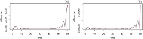
As we can see in Figure 4, the solution obtained with the new algorithm is nearly the same that the one obtained with the IPOPT.

In order to have a better perception of the accuracy of the algorithm, we run it again with $\mathrm{tolerance}={10}^{-11}$, we take the obtained solution as the ‘real’ one in each case, and we compare the previous solution with the one obtained now. The difference between both solutions can be analysed in Figure 5.

Figure 5. Difference between the two solutions obtained using the variation of the indirect shooting method, in $x_1\left(t\right)$ (A) and $x_2\left(t\right)$ (B).

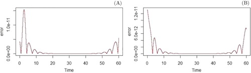
As it can be appreciated, the new algorithm shows to be quite accurate.

5. Conclusions

We have shown how the Turnpike phenomenon arises in the predator–prey system with a constrained control. Besides that, we have used this property to improve the classic single shooting method, following the ideas in [36]. The obtained solution has been checked with the one obtained with the IPOPT to compare the accuracy of the new method.

We would like to attract the attention on the importance of the concept of the turnpike. First, because it gives reach information about the shape of the solution of the optimal control problem (as it has been shown in Section 3). Secondly, due to the resulting efficiency of the variant of the showing method using the turnpike to compute numerically optimal solutions.

Optimal control problems defined on infinite time intervals or on large time intervals arise in many real problems, as in engineering, in models of economic growth, or in thermodynamical problems. Accurate numerical schemes are needed to solve this kind of problems since a small error can negatively affect the accuracy of the final solution. Consequently, the frame of possible applications of the Turnpike Theory could be huge.

On the other hand, the usefulness of the Turnpike property is reinforced by its robustness with respect to the changes in the initial conditions and the length of the time interval, as shown in Section 3.4. In addition, the Turnpike Theory allows freedom of designing the cost function in order to have the most convenient ‘Turnpike’ in the solution, as mentioned in Section 3.3.

As it has been explained in Remark 2.1 of Section 3.1, the Turnpike theorem of Trélat and Zuazua [36], which is the basis of the present work, is only applicable for optimal control problems without constraints on the control. When the control is unconstrained, the optimal control problem (8(3) $x_1\left(0\right)=x_1^0,x_2\left(0\right)=x_2^0,$(3) )–(11(11) $T=60$(11) ) with cost function (12(12) $\underset{u_{[0,1]}\in L^2(0,T;[0,1\left]\right)}{min}\frac{1}{2}{\int }_0^{\mathrm{T}}\left(\right(x_1\left(t\right)-1{)}^2+x_2(t{)}^2+u_{[0,1]}(t{)}^2)\mathrm{d}t.$(12) ) satisfies the Turnpike theorem we cite on Section 2.2. Even if we have not proved analytically that Theorem 1 is valid for the problem with constrained control, simulations of Section 3 show that the turnpike property holds.

We would like to remark that the analytic proof of the turnpike theorem with control constraints is a not trivial open probel, and actually, it is the main direction for the immediate future work. Even if there are turnpike results for optimal control problems with constrained control (see, for example, [10] or [6]), to our best knowledge, there are not turnpike results with constrained control, proving that the adjoint verifies the turnpike.

However, in this work we show through simulations that the Turnpike Theory of Trélat and Zuazua [36], which involves the adjoint besides the state and the control, is also true when there are constraints in the control, which brings up an interesting open problem.

Acknowledgments

I am very grateful to Prof. Enrique Zuazua for his guidance and advise during this work.

I thank the anonymous reviewers for their interesting suggestions – in particular, for pointing out the open problem of the turnpike phenomenon in optimal control problems with control constrains.

I warmly thank Ander Murua for his help with the computational issues and Ramón Escobedo for his advice. Thanks are also due to Emmanuel Trélat, Alejandro Pozo, Aurora Marica, Jérôme Lohéac, Navid Allahverdi and Felipe Chaves-Silva for their help.

I deeply appreciate Inderpreet Kaur and Umberto Biccari for his assistance with English language editing of this manuscript. This work was done in the framework of the research group ‘Partial differential equations, numerics and control’ of BCAM (Basque Center for Applied Mathematics).

Disclosure statement

No potential conflict of interest was reported by the authors.

ORCiD

Aitziber Ibañez http://orcid.org/0000-0001-5523-7521

Additional information

Funding

This work was supported by the Advanced Grant NUMERIWAVES/FP7-246775 of the European Research Council Executive Agency, the BERC 2014–2017 programme of the Basque Government, the MTM2014-52347 and MTM2011-29306 Grants and the Severo Ochoa programme SEV-2013-0323 of the MINECO.

Appendix A.

The optimal control problem to be solved is to find a control $u(\cdot )\in L^2(0,T,[0,1\left]\right)$ satisfying: (A1) $\frac{\mathrm{d}{x}_1\left(t\right)}{\mathrm{d}t}=x_1\left(t\right)-x_1\left(t\right)x_2\left(t\right)-0.4x_1\left(t\right)u_{[0,1]}\left(t\right),$(A1) (A2) $\frac{\mathrm{d}{x}_2\left(t\right)}{\mathrm{d}t}=-x_2\left(t\right)+x_1\left(t\right)x_2\left(t\right)-0.2x_2\left(t\right)u_{[0,1]}\left(t\right),$(A2) (A3) $\left(x_1\right(0),x_2(0\left)\right)=(0.5;0.7),$(A3) (A4) $T=60,$(A4) which minimises the following cost function: (A5) $\underset{u(\cdot )\in L^2(0,T,[0,1\left]\right)}{min}\frac{1}{2}{\int }_0^{\mathrm{T}}\left(\right(x_1\left(t\right)-1{)}^2+x_2(t{)}^2+u_{[0,1]}(t{)}^2)\mathrm{d}t$(A5)

Let denote by $\left(x_T\right(\cdot ),u_T(\cdot \left)\right)$ an optimal solution of Equation (A4). Then, according to the Pontryagin maximum principle (Section 7.2 of Trélat [34]), there exists an absolutely continuous mapping $p_T(\cdot ):[0,T]\to {\mathbb{R}}^2$, called the adjoint vector, and a real number $p_T^0\le 0$, such that, for almost every $t\in [0,T]$: (A6) ${\dot{x}}_T\left(t\right)=\frac{\mathrm{\partial }H}{\mathrm{\partial }p}(x_T,p_T,p_T^0,u_T),$(A6) (A7) ${\dot{p}}_T\left(t\right)=-\frac{\mathrm{\partial }H}{\mathrm{\partial }x}(x_T,p_T,p_T^0,u_T),$(A7) where H is the Hamiltonian of the problem defined as $H=⟨p,f⟩+p^0{f}^0$, satisfying: (A8) $\begin{array}{r}H\left(x_T\right(t),p_T(t),p_T^0,u_T(t\left)\right)=\underset{v\left(t\right)\in L^2(0,T;[0,1\left]\right)}{max}H\left(x_T\right(t),p_T(t),p_T^0,v(t\left)\right).\end{array}$(A8)

The Hamiltonian is (A9) $H=p_1(x_1-x_1{x}_2-0.4x_1{u}_{[0,1]})+p_2(-x_2+x_1{x}_2-0.2x_2{u}_{[0,1]})-\frac{1}{2}\left(\right(x_1-1{)}^2+x_2^2+u_{[0,1]}^2)$(A9)

Then, from the application of the Pontryagin maximum principle, we get the adjoint vector: (A10) $\begin{array}{rl}\dot{p_1}& =(-1+0.4u_{[0,1]})p_1+x_2(p_1-p_2)+(x_1-1),\\ \dot{p_2}& =(1+0.2u_{[0,1]})p_2+x_1(p_1-p_2)+x_2\end{array}$(A10) from the Hamiltonian maximization condition: (A11) $u_{[0,1]}=\left\{\begin{array}{ll}0& if-0.4x_1{p}_1-0.2p_2{x}_2<0,\\ -0.4x_1{p}_1-0.2p_2{x}_2& if0\le -0.4x_1{p}_1-0.2p_2{x}_2\le 1,\\ 1& if-0.4x_1{p}_1-0.2p_2{x}_2>1\end{array}\right.$(A11) and, finally, from the transversal condition: $\left(p_1\right(T),p_2(T\left)\right)=(0,0)$.

Then, we get the following boundary problem: (A12) $\left\{\begin{array}{l}\dot{x_1}=x_1-x_1{x}_2-0.4x_{1}u,\\ \dot{x_2}=-x_2+x_1{x}_2-0.2x_{2}u,\\ \dot{p_1}=(-1+0.4u)p_1+x_2(p_1-p_2)+(x_1-1),\\ \dot{p_2}=(1+0.2u)p_2+x_1(p_1-p_2)+x_2,\\ \left(x_1\right(0),x_2(0),p_1(T),p_2(T\left)\right)=(0.5,0.7,0,0),\end{array}\right.$(A12)

where u is the piecewise function defined in (A11).

Let define the boundary function: (A13) $G\left(\right(x\left(T/2\right),y\left(T/2\right),p_1\left(T/2\right),p_2\left(T/2\right))=(x\left(0\right)-0.5,x_2\left(0\right)-0.7,p_1\left(T\right),p_2\left(T\right)).$(A13)

The algorithm to solve the type optimal control problem (A1)–(A4) with cost function (A5), following the idea explained in [36] is $\begin{array}{rl}& \mathrm{\Delta }G\left(\right(x_1\left(T/2\right),x_2\left(T/2\right),p_1\left(T/2\right),p_2\left(T/2\right))\\ & =\frac{1}{ϵ}{\left(\begin{array}{c}G\left(\right(x_1\left(T/2\right)+ϵ,x_2\left(T/2\right),p_1\left(T/2\right),p_2\left(T/2\right))-G(\left(x_1\right(T/2),x_2(T/2),p_1(T/2),p_2(T/2\left)\right)\\ G\left(\right(x_1\left(T/2\right),x_2\left(T/2\right)+ϵ,p_1\left(T/2\right),p_2\left(T/2\right))-G(\left(x_1\right(T/2),x_2(T/2),p_1(T/2),p_2(T/2\left)\right)\\ G\left(\right(x_1\left(T/2\right),x_2\left(T/2\right),p_1\left(T/2\right)+ϵ,p_2\left(T/2\right))-G(\left(x_1\right(T/2),x_2(T/2),p_1(T/2),p_2(T/2\left)\right)\\ G\left(\right(x_1\left(T/2\right),x_2\left(T/2\right),p_1\left(T/2\right),p_2\left(T/2\right)+ϵ)-G(\left(x_1\right(T/2),x_2(T/2),p_1(T/2),p_2(T/2\left)\right)\end{array}\right)}^{\mathrm{T}}.\end{array}$

• Input: $G\left(s\right)$ (boundary function), $F\left(s\right)$ (differential system), ε, maxiter (maximal number of iterations), T, N (number of time steps to solve the ODE system ), tol1 (tolerance for the method used to solve the differential system), tol2 (tolerance for the Newton method), $(\overline{x_1},\overline{x_2},\overline{p_1},\overline{p_2})$ (the turnpike previously calculated)

• Initialize $z(T/2{)}^{\left(0\right)}=(x_1\left(T/2\right),x_2\left(T/2\right),p_1\left(T/2\right),p_2\left(T/2\right))=(\overline{x_1},\overline{x_2},\overline{p_1},\overline{p_2})$, i=1

• Calculate $\left(x_1\right(0),x_2(0){)}^{\left(0\right)}$ integrating backwards the system $\dot{z}=F\left(z\right)$ in $[0,T/2]$ using the initial point $z(T/2{)}^{\left(0\right)}$

• Calculate $\left(p_1\right(T),p_2(T\left)\right)$ integrating the system $\dot{z}=F\left(z\right)$ in $[T/2,T]$ using the initial point $z(T/2{)}^{\left(0\right)}$

• While the $i<\mathrm{maxiter}$ and $\mathrm{error}>\mathrm{tol}2$ do:

  1. Calculate $G\left(z\right(T/2{)}^{\left(i\right)})$ and $\mathrm{\Delta }G\left(z\right(T/2{)}^{\left(i\right)})$

  2. Calculate $z(T/2{)}^{(i+1)}$: $z(T/2{)}^{(i+1)}=z(T/2{)}^{\left(i\right)}-\left(\mathrm{\Delta }G\right(z\left(T/2{)}^{\left(i\right)}\right){)}^{-1}.G\left(z\right(T/2{)}^{\left(i\right)})$

  3. $\mathrm{error}=|G\left(z\right(T/2{)}^{\left(i\right)})|$and i=i+1

• Calculate the optimal solution using the point $z(T/2{)}^{\left(i\right)}$ integrating backwards and forwards.

• Calculate the control $u_{[0,1]}\left(t\right)$ using the Hamiltonian maximization condition

• Output: $\left(x\right(t),u(t\left)\right)$, the error and the number of iteration

This algorithm has been implemented using the free software R [26]. Runge–Kutta method of order 4 was chosen to integrate forward and backward (with error tolerance=${10}^{-9}$). We used the following parameters to run the algorithm: $ϵ={10}^{-10},\mathrm{maxiter}=100,\mathrm{tol}1=\mathrm{tol}2={10}^{-9}$

The error of this solution is $2.378833\times {10}^{-11}$ , and it has been necessary to do six iterations. Runge–Kutta method of order 4 was chosen to integrate forward and backward. The algorithm was run on a personal laptop of 2 cores and 4 GB of RAM memory, and it took 771 seconds to solve the problem.

References

- B.D. Anderson and P.V. Kokotovic, Optimal control problems over large time intervals, Automatica 23 (1987), pp. 355–363. doi: 10.1016/0005-1098(87)90008-2
- N. Apreutesei and G. Dimitriu, Optimal control for Lotka–Volterra systems with a hunter population, in International Conference on Large-Scale Scientific Computing, Springer, Berlin, 2008, pp. 277–284.
- E.N. Bodine, L.J. Gross, and S. Lenhart, Optimal control applied to a model for species augmentation, Math. Biosci. Eng. 5 (2008), pp. 669–680. doi: 10.3934/mbe.2008.5.669
- F. Brauer and C. Castillo-Chavez, Mathematical Models in Population Biology and Epidemiology, Springer, New York, 2011.
- R. Bulirsch and J. Stoer, Introduction to Numerical Analysis, Springer, Heidelberg, 2002.
- D.A. Carlson, A. Haurie, and A. Leizarowitz, Infinite Horizon Optimal Control: Deterministic and Stochastic Systems, Springer-Verlag, Berlin, 2012.
- L. Crespo and J. Sun, Optimal control of populations of competing species, Nonlinear Dyn. 27 (2002), pp. 197–210. doi: 10.1023/A:1014258302180
- T. Damm, L. Grüne, M. Stieler, and K. Worthmann, An exponential turnpike theorem for dissipative discrete time optimal control problems, SIAM J. Control Optim. 52 (2014), pp. 1935–1957. doi: 10.1137/120888934
- T. Faulwasser, M. Korda, C.N. Jones, and D. Bonvin, On Turnpike and Dissipativity Properties of Continuous-Time Optimal Control Problems, preprint (2015). Available at arXiv:1509.07315.
- R. Fourer, D. Gay, and B. Kernighan, Ampl: A Modeling Language for Mathematical Programming, 2nd ed., Brooks/Cole-Thomson Learning, Pacific Grove, CA, 2003.
- L. Grüne, Economic receding horizon control without terminal constraints, Automatica 49 (2013), pp. 725–734. doi: 10.1016/j.automatica.2012.12.003
- A. Ibañez, Optimal control and turnpike properties of the Lotka–Volterra model, Master Thesis, Universidad del País Vasco/Euskal Herriko Unibertsitatea. Available at http://www.bcamath.org/documentos_public/archivos/personal/conferencias/LotkaVolterra.pdf.
- A.F. Ivanov, M.A. Mammadov, and S.I. Trofimchuk, Global stabilization in nonlinear discrete systems with time-delay, J. Global Optim. 56 (2013), pp. 251–263. doi: 10.1007/s10898-012-9862-y
- M. Jaberi-Douraki and S.M. Moghadas, Optimal control of vaccination dynamics during an influenza epidemic, Math. Biosci. Eng. 11 (2014), pp. 1045–1063. doi: 10.3934/mbe.2014.11.1045
- U. Ledzewicz, H. Maurer, and H. Schaettler, Optimal and suboptimal protocols for a mathematical model for tumor anti-angiogenesis in combination with chemotherapy, Math. Biosci. Eng. 8 (2011), pp. 307–323. doi: 10.3934/mbe.2011.8.307
- U. Ledzewicz, A. d'Onofrio, and H. Schättler, Tumor Development Under Combination Treatments with anti-angiogenic therapies, Springer, New York, 2013.
- S. Lee, G. Chowell, and C. Castillo-Chávez, Optimal control for pandemic influenza: The role of limited antiviral treatment and isolation, J. Theoret. Biol. 265 (2010), pp. 136–150. doi: 10.1016/j.jtbi.2010.04.003
- A.J. Lotka, Elements of Physical Biology, Williams and Wilkins, Baltimore, 1925.
- M.V. Martinez, S. Lenhart, and K.A.J. White, Optimal control of integrodifference equations in a pest-pathogen system, Discret. Contin. Dyn. Syst. – Ser. B 20 (2015), pp. 1759–1783. http://aimsciences.org/journals/displayArticlesnew.jsp?paperID=11231. doi: 10.3934/dcdsb.2015.20.1759
- L.W. McKenzie, The turnpike theorem of morishima (1), Metroeconomica 15 (1963), pp. 146–154. doi: 10.1111/j.1467-999X.1963.tb00308.x
- L.W. McKenzie, Turnpike theorems for a generalized Leontief model, Econometrica: J. Econometr.Soc. 31 (1963), pp. 165–180. doi: 10.2307/1910955
- M. Morishima, Proof of a turnpike theorem: The ‘no joint production case’, Rev. Econ. Stud. 1961, pp. 89–97. doi: 10.2307/2295706
- A. Porretta and E. Zuazua, Long time versus steady state optimal control, SIAM J. Control Optim. 51 (2013), pp. 4242–4273. doi: 10.1137/130907239
- R. Radner, Paths of economic growth that are optimal with regard only to final states: A turnpike theorem, Rev. Econ. Stud. 28(1961), pp. 98–104. doi: 10.2307/2295707
- R Development Core Team, R: A Language and Environment for Statistical Computing, R Foundation for Statistical Computing, Vienna Austria, 2008. http://www.R-project.org. ISBN 3-900051-07-0.
- S. Sager, H.G. Bock, M. Diehl, G. Reinelt, and J.P. Schloder, Numerical methods for optimal control with binary control functions applied to a Lotka–Volterra type fishing problem, in Recent Advances in Optimization. Vol. 563 of Lectures Notes in Economics and Mathematical Systems, A. Seeger, ed., Springer, Heidelberg, 2006, pp. 269–289.
- P.A. Samuelson, R. Dorfman and R.M. Solow, Linear Programming and Economic Analysis, McGraw-Hill, New York, 1958.
- S.H. Scott, Optimal strategies for movement: Success with variability, Nat. Neurosci. 5 (2002), pp. 1110–1111. doi: 10.1038/nn1102-1110
- S.H. Scott, Optimal feedback control and the neural basis of volitional motor control, Nat. Rev. Neurosci. 5 (2004), pp. 532–546. doi: 10.1038/nrn1427
- A. Swierniak, U. Ledzewicz, and H. Schattler, Optimal control for a class of compartmental models in cancer chemotherapy, Int. J. Appl. Math. Comput. Sci. 13 (2003), pp. 357–368.
- E. Todorov, Optimality principles in sensorimotor control, Nat. Neurosci. 7 (2004), pp. 907–915. doi: 10.1038/nn1309
- E. Todorov and M.I. Jordan, Optimal feedback control as a theory of motor coordination, Nat. Neurosci. 5 (2002), pp. 1226–1235. doi: 10.1038/nn963
- E. Trélat, Contrôle Optimal: Théorie & Applications, Vuibert, Paris, 2005.
- E. Trélat, Optimal control and applications to aerospace: Some results and challenges, J. Optim. Theory Appl. 154 (2012), pp. 713–758. doi: 10.1007/s10957-012-0050-5
- E. Trélat and E. Zuazua, The turnpike property in finite-dimensional nonlinear optimal control, J. Diff. Equ. 258 (2015), pp. 81–114. doi: 10.1016/j.jde.2014.09.005
- V. Volterra, Variazioni e fluttuazioni del numero d'individui in specie animali conviventi (C. Ferrari), (1927).
- A. Wächter and L.T. Biegler, On the implementation of an interior-point filter line-search algorithm for large-scale nonlinear programming, Math. Program. 106 (2006), pp. 25–57. doi: 10.1007/s10107-004-0559-y
- R. Wilde and P. Kokotovic, A dichotomy in linear control theory, IEEE Trans. Autom. Control 17 (1972), pp. 382–383. doi: 10.1109/TAC.1972.1099976
- S. Yosida, An optimal control problem of the prey–predator system, Funck. Ekvacioj 25 (1982), pp. 283–293.
- A. Zaslavski, Turnpike Properties in the Calculus of Variations and Optimal Control, Vol. 80. Springer, New York, 2006.