Mathematical analysis of an HIV latent infection model including both virus-to-cell infection and cell-to-cell transmission

ABSTRACT

HIV can infect cells via virus-to-cell infection or cell-to-cell viral transmission. These two infection modes may occur in a synergistic way and facilitate viral spread within an infected individual. In this paper, we developed an HIV latent infection model including both modes of transmission and time delays between viral entry and integration or viral production. We analysed the model by defining the basic reproductive number, showing the existence, positivity and boundedness of the solution, and proving the local and global stability of the infection-free and infected steady states. Numerical simulations have been performed to illustrate the theoretical results and evaluate the effects of time delays and fractions of infection leading to latency on the virus dynamics. The estimates of the relative contributions to the HIV latent reservoir and the virus population from the two modes of transmission have also been provided.

KEYWORDS:

• HIV infection
• latent reservoir
• cell-to-cell transmission
• time delay
• stability analysis

AMS SUBJECT CLASSIFICATION:

• 92B05
• 92D25
• 92C37
• 34D23

1. Introduction

Human immunodeficiency virus (HIV) is a retrovirus that mainly infects CD4${}^{+}$ T cells. Upon infection, CD4${}^{+}$ T cells can produce new virions, which lead to more cell infection and viral production. Many mathematical models have been developed to study the within-host dynamics of HIV infection [8, 16, 31–36, 41, 42, 53–55] . Most of these models were focused on the virus-to-cell infection. However, virus can also spread by direct cell-to-cell transmission [26, 29, 30, 45–48, 50, 57]. The mechanisms underlying the cell-to-cell transmission are not completely clear. Virus may be transferred from infected cells to bystander uninfected cells via the formation of virological synapses [17]. Comparing with the cell-free virus infection, cell-to-cell transmission may have some advantages for viral spread [3, 45, 60]. For example, virus transmitted via cell-to-cell transmission may have a lower risk of being neutralized by neutralizing antibodies or cleared by cytotoxic T lymphocytes [27]. Moreover, a number of virions can be transferred to a target cell simultaneously and the probability of being completely blocked by antiretroviral therapy is lower. Thus, cell-to-cell spread of HIV may explain the viral load persistence during effective combination therapy [49]. The relative contributions to the viral replication from the two modes of transmission still remain unclear [5, 6, 18, 19, 38, 59].

Mathematical models have been used to study the dynamics of HIV infection including these two transmission modes [18–22, 24, 25, 39, 58]. A recent review on modelling viral spread can be found in Ref. [12]. Iwami et al. [18] and Komarova et al. [19] studied the relative contribution of the two transmission modes to the spread of HIV. Lai and Zou [24, 25] developed models that incorporate two modes of viral spread with and without the logistic target cell growth. They showed that the basic reproductive number determines the infection dynamics and that the logistic growth of target cells can generate a Hopf bifurcation. A within-host viral infection model with the two transmission modes and three distributed delays was analysed in Ref. [58]. A multi-strain model including the two modes was also analysed and shown to exhibit a competitive exclusion principle [39].

Current treatment consisting of several antiretroviral drugs can suppress viral replication to a low level but cannot eradicate the virus. An important reason is that HIV provirus can reside in latently infected CD4${}^{+}$ T cells [7, 56]. Latently infected CD4${}^{+}$ T cells live long, are not affected by antiretroviral drugs or immune responses, but can be activated to produce virus by relevant antigens. In the present paper, on the basis of the models by Lai and Zou [24, 25] and Alshorman et al. [2], we developed an HIV latent infection model incorporating both the cell-free virus infection and cell-to-cell transmission. Two delays, one the time between viral entry and viral DNA integration into the host cell's DNA and the other the time between viral entry and viral production, have also been included in the model. We analysed the model by deriving the basic reproductive number and showing the local and global stability of the steady states. We also performed numerical simulations to explore the effects of time delays and other parameters on virus dynamics and estimate the relative contributions to the latent reservoir and viral load from the two modes of viral transmission.

2. Model formulation

We considered both the virus-to-cell infection and cell-to-cell transmission in an HIV latent infection model [34]. Two time delays were included in our model. The first delay (${\tau }_1$) is the time between viral entry and latent infection, that is, the time between initial viral infection and the integration of viral DNA into the host cell's DNA. The second (${\tau }_2$) is the time between cell infection and viral production. It is clear that ${\tau }_1<{\tau }_2$ according to the viral life cycle. As assumed in HIV latent infection models [2, 34, 43, 44], a very small fraction of CD4${}^{+}$ T cell infection leads to HIV latency. They don't produce new virus unless activated by antigens. The model can be described by the following delayed differential equations: (1) $\begin{array}{rl}\frac{\mathrm{d}T\left(t\right)}{\mathrm{d}t}& =s-d_{T}T\left(t\right)-\beta T\left(t\right)V\left(t\right)-kT\left(t\right)I\left(t\right),\\ \frac{\mathrm{d}L\left(t\right)}{\mathrm{d}t}& =f\beta T(t-{\tau }_1)V(t-{\tau }_1){\mathrm{e}}^{-{\delta }_1{\tau }_1}+\eta kT(t-{\tau }_1)I(t-{\tau }_1){\mathrm{e}}^{-{\delta }_1{\tau }_1}\\ & -(\alpha +{\delta }_L)L\left(t\right),\\ \frac{\mathrm{d}I\left(t\right)}{\mathrm{d}t}& =(1-f)\beta T(t-{\tau }_2)V(t-{\tau }_2){\mathrm{e}}^{-{\delta }_1{\tau }_2}+(1-\eta )kT(t-{\tau }_2)I(t-{\tau }_2){\mathrm{e}}^{-{\delta }_1{\tau }_2}\\ & -\delta I\left(t\right)+\alpha L\left(t\right),\\ \frac{\mathrm{d}V\left(t\right)}{\mathrm{d}t}& =N\delta I\left(t\right)-cV\left(t\right),\end{array}$(1) where $T\left(t\right)$ denotes the concentration of uninfected CD4${}^{+}$ T cells at time t, $L\left(t\right)$ represents the concentration of latently infected T cells at time t, $I\left(t\right)$ is the concentration of productively infected T cells, and $V\left(t\right)$ denotes the concentration of virions in plasma. The model assumes that uninfected CD4${}^{+}$ T cells are produced at a rate s, infected by free virus at a rate β or by direct cell-to-cell transmission at a rate k. Parameter $d_T$ is the per capita death rate of uninfected CD4${}^{+}$ T cells. The constants $f,\eta \in (0,1)$ are the proportions of infection that lead to latency. Latently infected cells die at a rate ${\delta }_L$ per cell and productively infected cells die at a rate δ per cell. Latently infected cells can be activated by their relevant antigens to become productively infected cells at a rate α. Proliferation of latently infected cells is not considered here but can be added to the model as in [43]. N is the viral burst size, that is, the total number of virions released by one infected cell during its lifespan, and c is the viral clearance rate. The parameter ${\delta }_1$ is the death rate of infected cells in which viral DNA has not integrated into the host cell's DNA. Thus, ${\mathrm{e}}^{-{\delta }_1{\tau }_1}$ and ${\mathrm{e}}^{-{\delta }_1{\tau }_2}$ represent the probability of an infected cell surviving to the age of ${\tau }_1$ and ${\tau }_2$, respectively.

We define the following Banach space [13, 23]: $\begin{array}{rl}C& =\{\phi \in C((-\mathrm{\infty },0],R\left)|\phi \right(\theta ){\mathrm{e}}^{l\theta }\text{is uniformly continuous for}\\ & \times \theta \in (-\mathrm{\infty },0]\text{and}\Vert \phi \Vert <\mathrm{\infty }\},\end{array}$ where l is a positive constant and the norm in the space is $\Vert \phi \Vert =\underset{\theta \le 0}{sup}|\phi \left(\theta \right)|{\mathrm{e}}^{l\theta }.$

The set $C_{+}=C\left(\right(-\mathrm{\infty },0],R_{+})$ is the non-negative cone of C. For a given function $\varphi \left(t\right)=\left(T\right(t),L(t),I(t),V(t\left)\right)$, we let $\begin{array}{rl}{\varphi }_t\left(\theta \right)& =\left(T_t\right(\theta ),L_t(\theta ),I_t(\theta ),V_t(\theta \left)\right)=\varphi (t+\theta )\\ & =\left(T\right(t+\theta ),L(t+\theta ),I(t+\theta ),V(t+\theta \left)\right),\theta \in (-\mathrm{\infty },0].\end{array}$ The initial conditions are given by (2) $(T_0,L_0,I_0,V_0)\in C_{+}^4=C_{+}\times C_{+}\times C_{+}\times C_{+}.$(2) By the fundamental theory of functional differential equations [14, 23], we can obtain the existence and uniqueness of the solution for t>0.

2.1. Positivity and boundedness of solution

The following result shows that a solution $\left(T\right(t),L(t),I(t),V(t\left)\right)$ of system (1(1) $\begin{array}{rl}\frac{\mathrm{d}T\left(t\right)}{\mathrm{d}t}& =s-d_{T}T\left(t\right)-\beta T\left(t\right)V\left(t\right)-kT\left(t\right)I\left(t\right),\\ \frac{\mathrm{d}L\left(t\right)}{\mathrm{d}t}& =f\beta T(t-{\tau }_1)V(t-{\tau }_1){\mathrm{e}}^{-{\delta }_1{\tau }_1}+\eta kT(t-{\tau }_1)I(t-{\tau }_1){\mathrm{e}}^{-{\delta }_1{\tau }_1}\\ & -(\alpha +{\delta }_L)L\left(t\right),\\ \frac{\mathrm{d}I\left(t\right)}{\mathrm{d}t}& =(1-f)\beta T(t-{\tau }_2)V(t-{\tau }_2){\mathrm{e}}^{-{\delta }_1{\tau }_2}+(1-\eta )kT(t-{\tau }_2)I(t-{\tau }_2){\mathrm{e}}^{-{\delta }_1{\tau }_2}\\ & -\delta I\left(t\right)+\alpha L\left(t\right),\\ \frac{\mathrm{d}V\left(t\right)}{\mathrm{d}t}& =N\delta I\left(t\right)-cV\left(t\right),\end{array}$(1) ) with the initial condition (2) remains non-negative and bounded ultimately.

Theorem 2.1.

Let $\left(T\right(t),L(t),I(t),V(t\left)\right)$ be a solution of system (1(1) $\begin{array}{rl}\frac{\mathrm{d}T\left(t\right)}{\mathrm{d}t}& =s-d_{T}T\left(t\right)-\beta T\left(t\right)V\left(t\right)-kT\left(t\right)I\left(t\right),\\ \frac{\mathrm{d}L\left(t\right)}{\mathrm{d}t}& =f\beta T(t-{\tau }_1)V(t-{\tau }_1){\mathrm{e}}^{-{\delta }_1{\tau }_1}+\eta kT(t-{\tau }_1)I(t-{\tau }_1){\mathrm{e}}^{-{\delta }_1{\tau }_1}\\ & -(\alpha +{\delta }_L)L\left(t\right),\\ \frac{\mathrm{d}I\left(t\right)}{\mathrm{d}t}& =(1-f)\beta T(t-{\tau }_2)V(t-{\tau }_2){\mathrm{e}}^{-{\delta }_1{\tau }_2}+(1-\eta )kT(t-{\tau }_2)I(t-{\tau }_2){\mathrm{e}}^{-{\delta }_1{\tau }_2}\\ & -\delta I\left(t\right)+\alpha L\left(t\right),\\ \frac{\mathrm{d}V\left(t\right)}{\mathrm{d}t}& =N\delta I\left(t\right)-cV\left(t\right),\end{array}$(1) ) with the initial condition (2). It is positive and ultimately bounded for t>0.

Proof.

We first show that $T\left(t\right)>0$ for all t>0. Assume that there exists a $t_1>0$ such that $T\left(t_1\right)=0,T\left(t\right)>0,t\in [0,t_1)$. Thus, $\dot{T}\left(t_1\right)\le 0$. From the first equation of (1(1) $\begin{array}{rl}\frac{\mathrm{d}T\left(t\right)}{\mathrm{d}t}& =s-d_{T}T\left(t\right)-\beta T\left(t\right)V\left(t\right)-kT\left(t\right)I\left(t\right),\\ \frac{\mathrm{d}L\left(t\right)}{\mathrm{d}t}& =f\beta T(t-{\tau }_1)V(t-{\tau }_1){\mathrm{e}}^{-{\delta }_1{\tau }_1}+\eta kT(t-{\tau }_1)I(t-{\tau }_1){\mathrm{e}}^{-{\delta }_1{\tau }_1}\\ & -(\alpha +{\delta }_L)L\left(t\right),\\ \frac{\mathrm{d}I\left(t\right)}{\mathrm{d}t}& =(1-f)\beta T(t-{\tau }_2)V(t-{\tau }_2){\mathrm{e}}^{-{\delta }_1{\tau }_2}+(1-\eta )kT(t-{\tau }_2)I(t-{\tau }_2){\mathrm{e}}^{-{\delta }_1{\tau }_2}\\ & -\delta I\left(t\right)+\alpha L\left(t\right),\\ \frac{\mathrm{d}V\left(t\right)}{\mathrm{d}t}& =N\delta I\left(t\right)-cV\left(t\right),\end{array}$(1) ), we have $\dot{T}\left(t_1\right)=s>0$, which is a contradiction. This implies that $T\left(t\right)>0$ for all t>0.

By the last three equations of system (1(1) $\begin{array}{rl}\frac{\mathrm{d}T\left(t\right)}{\mathrm{d}t}& =s-d_{T}T\left(t\right)-\beta T\left(t\right)V\left(t\right)-kT\left(t\right)I\left(t\right),\\ \frac{\mathrm{d}L\left(t\right)}{\mathrm{d}t}& =f\beta T(t-{\tau }_1)V(t-{\tau }_1){\mathrm{e}}^{-{\delta }_1{\tau }_1}+\eta kT(t-{\tau }_1)I(t-{\tau }_1){\mathrm{e}}^{-{\delta }_1{\tau }_1}\\ & -(\alpha +{\delta }_L)L\left(t\right),\\ \frac{\mathrm{d}I\left(t\right)}{\mathrm{d}t}& =(1-f)\beta T(t-{\tau }_2)V(t-{\tau }_2){\mathrm{e}}^{-{\delta }_1{\tau }_2}+(1-\eta )kT(t-{\tau }_2)I(t-{\tau }_2){\mathrm{e}}^{-{\delta }_1{\tau }_2}\\ & -\delta I\left(t\right)+\alpha L\left(t\right),\\ \frac{\mathrm{d}V\left(t\right)}{\mathrm{d}t}& =N\delta I\left(t\right)-cV\left(t\right),\end{array}$(1) ), we have $\begin{array}{rl}L\left(t\right)& =L\left(0\right){\mathrm{e}}^{-(\alpha +{\delta }_L)t}+{\int }_0^t\left(f\beta T\right(\xi -{\tau }_1\left)V\right(\xi -{\tau }_1){\mathrm{e}}^{-{\delta }_1{\tau }_1}\\ & +\eta kT(\xi -{\tau }_1)I(\xi -{\tau }_1){\mathrm{e}}^{-{\delta }_1{\tau }_1}){\mathrm{e}}^{-(\alpha +{\delta }_L)(t-\xi )}\mathrm{d}\xi ,\\ I\left(t\right)& =I\left(0\right){\mathrm{e}}^{-\delta t}+{\int }_0^t\left[\right(1-f\left)\beta T\right(\xi -{\tau }_2\left)V\right(\xi -{\tau }_2){\mathrm{e}}^{-{\delta }_1{\tau }_2}\\ & +(1-\eta )kT(\xi -{\tau }_2)I(\xi -{\tau }_2){\mathrm{e}}^{-{\delta }_1{\tau }_2}+\alpha L\left(\xi \right)]{\mathrm{e}}^{-\delta (t-\xi )}\mathrm{d}\xi ,\\ V\left(t\right)& =V\left(0\right){\mathrm{e}}^{-ct}+{\int }_0^{t}N\delta I\left(\xi \right){\mathrm{e}}^{-c(t-\xi )}\mathrm{d}\xi ,\end{array}$ which shows that $L\left(t\right)>0,I\left(t\right)>0,V\left(t\right)>0$ for a small t>0. Now, we prove that $L\left(t\right)>0,I\left(t\right)>0,V\left(t\right)>0$ for all t>0. Assume that $t_2>0$ is the first time such that $min\left\{L\right(t_2),I(t_2),V(t_2\left)\right\}=0.$ If $L\left(t_2\right)=0,L\left(t\right)>0$ for $t\in [0,t_2)$ and $I\left(t\right)>0,V\left(t\right)>0,t\in [0,t_2]$, then we have $\dot{L}\left(t_2\right)\le 0$. On the other hand, from the second equation of (1(1) $\begin{array}{rl}\frac{\mathrm{d}T\left(t\right)}{\mathrm{d}t}& =s-d_{T}T\left(t\right)-\beta T\left(t\right)V\left(t\right)-kT\left(t\right)I\left(t\right),\\ \frac{\mathrm{d}L\left(t\right)}{\mathrm{d}t}& =f\beta T(t-{\tau }_1)V(t-{\tau }_1){\mathrm{e}}^{-{\delta }_1{\tau }_1}+\eta kT(t-{\tau }_1)I(t-{\tau }_1){\mathrm{e}}^{-{\delta }_1{\tau }_1}\\ & -(\alpha +{\delta }_L)L\left(t\right),\\ \frac{\mathrm{d}I\left(t\right)}{\mathrm{d}t}& =(1-f)\beta T(t-{\tau }_2)V(t-{\tau }_2){\mathrm{e}}^{-{\delta }_1{\tau }_2}+(1-\eta )kT(t-{\tau }_2)I(t-{\tau }_2){\mathrm{e}}^{-{\delta }_1{\tau }_2}\\ & -\delta I\left(t\right)+\alpha L\left(t\right),\\ \frac{\mathrm{d}V\left(t\right)}{\mathrm{d}t}& =N\delta I\left(t\right)-cV\left(t\right),\end{array}$(1) ), we have $\dot{L}\left(t_2\right)=f\beta T(t_2-{\tau }_1)V(t_2-{\tau }_1){\mathrm{e}}^{-{\delta }_1{\tau }_1}+\eta KT(t_2-{\tau }_1)I(t_2-{\tau }_1){\mathrm{e}}^{-{\delta }_1{\tau }_1}>0.$ This leads to a contradiction.

If $I\left(t_2\right)=0,I\left(t\right)>0$ for $t\in [0,t_2)$ and $L\left(t\right)>0,V\left(t\right)>0,t\in [0,t_2]$, we also have $\dot{I}\left(t_2\right)\le 0$. However, from the third equation, we have $\begin{array}{rl}\dot{I}\left(t_2\right)& =(1-f)\beta T(t_2-{\tau }_2)V(t_2-{\tau }_2){\mathrm{e}}^{-{\delta }_1{\tau }_2}\\ & +(1-\eta )kT(t_2-{\tau }_2)I(t_2-{\tau }_2){\mathrm{e}}^{-{\delta }_1{\tau }_2}+\alpha L\left(t_2\right)>0.\end{array}$ This also leads to a contradiction.

Similarly, we know that $V\left(t_2\right)=0$ is impossible. Thus, $T\left(t\right)>0,L\left(t\right)>0,I\left(t\right)>0$ and $V\left(t\right)>0$ for all t>0.

Next, we prove the boundedness of the solution of system (1(1) $\begin{array}{rl}\frac{\mathrm{d}T\left(t\right)}{\mathrm{d}t}& =s-d_{T}T\left(t\right)-\beta T\left(t\right)V\left(t\right)-kT\left(t\right)I\left(t\right),\\ \frac{\mathrm{d}L\left(t\right)}{\mathrm{d}t}& =f\beta T(t-{\tau }_1)V(t-{\tau }_1){\mathrm{e}}^{-{\delta }_1{\tau }_1}+\eta kT(t-{\tau }_1)I(t-{\tau }_1){\mathrm{e}}^{-{\delta }_1{\tau }_1}\\ & -(\alpha +{\delta }_L)L\left(t\right),\\ \frac{\mathrm{d}I\left(t\right)}{\mathrm{d}t}& =(1-f)\beta T(t-{\tau }_2)V(t-{\tau }_2){\mathrm{e}}^{-{\delta }_1{\tau }_2}+(1-\eta )kT(t-{\tau }_2)I(t-{\tau }_2){\mathrm{e}}^{-{\delta }_1{\tau }_2}\\ & -\delta I\left(t\right)+\alpha L\left(t\right),\\ \frac{\mathrm{d}V\left(t\right)}{\mathrm{d}t}& =N\delta I\left(t\right)-cV\left(t\right),\end{array}$(1) ) with the initial condition (2). From the positivity of the solution and the first equation of (1(1) $\begin{array}{rl}\frac{\mathrm{d}T\left(t\right)}{\mathrm{d}t}& =s-d_{T}T\left(t\right)-\beta T\left(t\right)V\left(t\right)-kT\left(t\right)I\left(t\right),\\ \frac{\mathrm{d}L\left(t\right)}{\mathrm{d}t}& =f\beta T(t-{\tau }_1)V(t-{\tau }_1){\mathrm{e}}^{-{\delta }_1{\tau }_1}+\eta kT(t-{\tau }_1)I(t-{\tau }_1){\mathrm{e}}^{-{\delta }_1{\tau }_1}\\ & -(\alpha +{\delta }_L)L\left(t\right),\\ \frac{\mathrm{d}I\left(t\right)}{\mathrm{d}t}& =(1-f)\beta T(t-{\tau }_2)V(t-{\tau }_2){\mathrm{e}}^{-{\delta }_1{\tau }_2}+(1-\eta )kT(t-{\tau }_2)I(t-{\tau }_2){\mathrm{e}}^{-{\delta }_1{\tau }_2}\\ & -\delta I\left(t\right)+\alpha L\left(t\right),\\ \frac{\mathrm{d}V\left(t\right)}{\mathrm{d}t}& =N\delta I\left(t\right)-cV\left(t\right),\end{array}$(1) ), we obtain $\frac{\mathrm{d}T\left(t\right)}{\mathrm{d}t}\le s-d_{T}T\left(t\right),$ which yields $\underset{t\to \mathrm{\infty }}{lim sup}T\left(t\right)\le \frac{s}{d_T}.$ Let $H\left(t\right)=(f+\eta )T\left(t\right)+L(t+{\tau }_1)e^{{\delta }_1{\tau }_1}.$ We have $\begin{array}{rl}\frac{\mathrm{d}H\left(t\right)}{\mathrm{d}t}& =(f+\eta )(s-d_{T}T(t)-\beta T(t\left)V\right(t)-kT(t\left)I\right(t\left)\right)\\ & +f\beta T\left(t\right)V\left(t\right)+\eta kT\left(t\right)V\left(t\right)-(\alpha +{\delta }_L)L(t+{\tau }_1){\mathrm{e}}^{{\delta }_1{\tau }_1}\\ & \le (f+\eta )s-(f+\eta )d_{T}T\left(t\right)-(\alpha +{\delta }_L)L(t+{\tau }_1){\mathrm{e}}^{{\delta }_1{\tau }_1}\\ & \le (f+\eta )s-\sigma H\left(t\right),\end{array}$ where $\sigma =min\{d_T,\alpha +{\delta }_L\}$. This yields $\underset{t\to \mathrm{\infty }}{lim sup}H\left(t\right)\le \frac{(f+\eta )s}{\sigma }.$ Thus, $\underset{t\to \mathrm{\infty }}{lim sup}L\left(t\right)\le \frac{(f+\eta )s}{\sigma }{\mathrm{e}}^{-{\delta }_1{\tau }_1}.$ Let $G\left(t\right)=\left(\right(1-f)+(1-\eta \left)\right)T\left(t\right)+I(t+{\tau }_2){\mathrm{e}}^{{\delta }_1{\tau }_2}.$ We obtain $\begin{array}{rl}\frac{\mathrm{d}G\left(t\right)}{\mathrm{d}t}& =\left(\right(1-f)+(1-\eta \left)\right)(s-d_{T}T(t)-\beta T(t\left)V\right(t)-kT(t\left)I\right(t\left)\right)\\ & +(1-f)\beta T\left(t\right)V\left(t\right)+(1-\eta )kT\left(t\right)I\left(t\right)-\delta I(t+{\tau }_2){\mathrm{e}}^{{\delta }_1{\tau }_2}+\alpha L(t+{\tau }_2){\mathrm{e}}^{{\delta }_1{\tau }_2}\\ & \le \left(\right(1-f)+(1-\eta \left)\right)s-\left(\right(1-f)+(1-\eta \left)\right)d_{T}T\left(t\right)-\delta I(t+{\tau }_2){\mathrm{e}}^{{\delta }_1{\tau }_2}\\ & +\frac{\alpha (f+\eta )s}{\sigma }{e}^{-{\delta }_1({\tau }_1-{\tau }_2)}\\ & \le a-bG\left(t\right),\end{array}$ where (3) $\begin{array}{rl}a& =\left(\right(1-f)+(1-\eta \left)\right)s+\frac{\alpha (f+\eta )s}{\sigma }{\mathrm{e}}^{-{\delta }_1({\tau }_1-{\tau }_2)},\\ b& =min\{d_T,\delta \}.\end{array}$(3) This implies that $\underset{t\to \mathrm{\infty }}{lim sup}G\left(t\right)\le \frac{a}{b}.$ Thus, $\underset{t\to \mathrm{\infty }}{lim sup}I\left(t\right)\le \frac{a}{b}{\mathrm{e}}^{-{\delta }_1{\tau }_2}.$ By the last equation of $V\left(t\right)$, we get $\frac{\mathrm{d}V\left(t\right)}{\mathrm{d}t}\le N\delta \cdot \frac{a}{b}{\mathrm{e}}^{-{\delta }_1{\tau }_2}-cV\left(t\right).$

Thus, $\underset{t\to \mathrm{\infty }}{lim sup}V\left(t\right)\le \frac{N\delta a{\mathrm{e}}^{-{\delta }_1{\tau }_2}}{bc}.$ Therefore, $T\left(t\right),L\left(t\right),I\left(t\right)$ and $V\left(t\right)$ are ultimately uniformly bounded.

Moreover, if we define $\begin{array}{rl}\mathrm{\Omega }& =\left\{(T,L,I,V)\in C_{+}^4:\Vert T\left(t\right)\Vert \le \frac{s}{d_T},\Vert L\left(t\right)\Vert \le \frac{(f+\eta )s}{\sigma }{e}^{-{\delta }_1{\tau }_1},\Vert I\left(t\right)\Vert \le \frac{a}{b}{\mathrm{e}}^{-{\delta }_1{\tau }_2},\right.\\ & \left.\Vert V\left(t\right)\Vert \le \frac{N\delta a{e}^{-{\delta }_1{\tau }_2}}{bc}\right\},\end{array}$ where a,b are given in Equation (3), then it follows from Theorem 2.1 that the region Ω is a positive invariant with respect to system (1(1) $\begin{array}{rl}\frac{\mathrm{d}T\left(t\right)}{\mathrm{d}t}& =s-d_{T}T\left(t\right)-\beta T\left(t\right)V\left(t\right)-kT\left(t\right)I\left(t\right),\\ \frac{\mathrm{d}L\left(t\right)}{\mathrm{d}t}& =f\beta T(t-{\tau }_1)V(t-{\tau }_1){\mathrm{e}}^{-{\delta }_1{\tau }_1}+\eta kT(t-{\tau }_1)I(t-{\tau }_1){\mathrm{e}}^{-{\delta }_1{\tau }_1}\\ & -(\alpha +{\delta }_L)L\left(t\right),\\ \frac{\mathrm{d}I\left(t\right)}{\mathrm{d}t}& =(1-f)\beta T(t-{\tau }_2)V(t-{\tau }_2){\mathrm{e}}^{-{\delta }_1{\tau }_2}+(1-\eta )kT(t-{\tau }_2)I(t-{\tau }_2){\mathrm{e}}^{-{\delta }_1{\tau }_2}\\ & -\delta I\left(t\right)+\alpha L\left(t\right),\\ \frac{\mathrm{d}V\left(t\right)}{\mathrm{d}t}& =N\delta I\left(t\right)-cV\left(t\right),\end{array}$(1) ).

2.2. The basic reproductive number and equilibria

System (1(1) $\begin{array}{rl}\frac{\mathrm{d}T\left(t\right)}{\mathrm{d}t}& =s-d_{T}T\left(t\right)-\beta T\left(t\right)V\left(t\right)-kT\left(t\right)I\left(t\right),\\ \frac{\mathrm{d}L\left(t\right)}{\mathrm{d}t}& =f\beta T(t-{\tau }_1)V(t-{\tau }_1){\mathrm{e}}^{-{\delta }_1{\tau }_1}+\eta kT(t-{\tau }_1)I(t-{\tau }_1){\mathrm{e}}^{-{\delta }_1{\tau }_1}\\ & -(\alpha +{\delta }_L)L\left(t\right),\\ \frac{\mathrm{d}I\left(t\right)}{\mathrm{d}t}& =(1-f)\beta T(t-{\tau }_2)V(t-{\tau }_2){\mathrm{e}}^{-{\delta }_1{\tau }_2}+(1-\eta )kT(t-{\tau }_2)I(t-{\tau }_2){\mathrm{e}}^{-{\delta }_1{\tau }_2}\\ & -\delta I\left(t\right)+\alpha L\left(t\right),\\ \frac{\mathrm{d}V\left(t\right)}{\mathrm{d}t}& =N\delta I\left(t\right)-cV\left(t\right),\end{array}$(1) ) is an autonomous differential equation system with fixed time delays. It always has an infection-free steady-state $E_0=(T_0,0,0,0)$, where $T_0=s/d_T$. Inspired by the method in Diekmann et al. [10] and van den Driessche and Watmough [52], we consider the infection and viral production, and define matrices $\mathbb{F}$ and $\mathbb{V}$ as $\mathbb{F}=\left(\begin{array}{ccc}0& \eta k{T}_0{\mathrm{e}}^{-{\delta }_1{\tau }_1}& f\beta T_0{\mathrm{e}}^{-{\delta }_1{\tau }_1}\\ 0& (1-\eta )k{T}_0{\mathrm{e}}^{-{\delta }_1{\tau }_2}& (1-f)\beta T_0{\mathrm{e}}^{-{\delta }_1{\tau }_2}\\ 0& 0& 0\end{array}\right)$ and $\mathbb{V}=\left(\begin{array}{ccc}\alpha +{\delta }_L& 0& 0\\ -\alpha & \delta & 0\\ 0& -N\delta & c\end{array}\right).$ Thus, the basic reproductive number, $R_0$, can be defined as the spectral radius of the next generation operator $\mathbb{F}{\mathbb{V}}^{-1}$, where $\mathbb{F}{\mathbb{V}}^{-1}=\left(\begin{array}{ccc}\left(\frac{\eta k}{\delta }+\frac{N\beta f}{c}\right)\frac{T_0\alpha {\mathrm{e}}^{-{\delta }_1{\tau }_1}}{\alpha +{\delta }_L}& \left(\frac{\eta k}{\delta }+\frac{N\beta f}{c}\right)T_0{\mathrm{e}}^{-{\delta }_1{\tau }_1}& \frac{f\beta T_0{\mathrm{e}}^{-{\delta }_1{\tau }_1}}{c}\\ \left(\frac{k(1-\eta )}{\delta }+\frac{N\beta (1-f)}{c}\right)\frac{T_0\alpha {\mathrm{e}}^{-{\delta }_1{\tau }_2}}{\alpha +{\delta }_L}& \left(\frac{k(1-\eta )}{\delta }+\frac{N\beta (1-f)}{c}\right)T_0{\mathrm{e}}^{-{\delta }_1{\tau }_2}& \frac{(1-f)\beta T_0{\mathrm{e}}^{-{\delta }_1{\tau }_2}}{c}\\ 0& 0& 0\end{array}\right).$

Therefore, $\begin{array}{rl}{R}_0& =\rho \left(\mathbb{F}{\mathbb{V}}^{-1}\right)=\frac{N\beta s}{c{d}_T}\left(\frac{\alpha f}{\alpha +{\delta }_L}{\mathrm{e}}^{-{\delta }_1{\tau }_1}+(1-f){\mathrm{e}}^{-{\delta }_1{\tau }_2}\right)\\ & +\frac{ks}{\delta d_T}\left(\frac{\alpha \eta }{\alpha +{\delta }_L}{\mathrm{e}}^{-{\delta }_1{\tau }_1}+(1-\eta ){\mathrm{e}}^{-{\delta }_1{\tau }_2}\right)\\ & \stackrel{\mathrm{\Delta }}{=}{R}_{01}+R_{02}.\end{array}$

For a within-host virus dynamic model, the basic reproduction number is the number of virions (or infected cells) produced by one virion (or one infected cell) in its lifespan in a fully susceptible environment (i.e. all the target cells are susceptible to virus infection). In the above expression of $R_0$, $N\beta s/\left(c{d}_T\right)$ is the basic reproduction number via the virus-to-cell infection and $ks/\left(\delta d_T\right)$ is the basic reproduction number via the cell-to-cell transmission. The first term in each parenthesis is the contribution of latent infection and the second term is the contribution of productive infection. Thus, $R_0$ is the basic reproduction number of system (1(1) $\begin{array}{rl}\frac{\mathrm{d}T\left(t\right)}{\mathrm{d}t}& =s-d_{T}T\left(t\right)-\beta T\left(t\right)V\left(t\right)-kT\left(t\right)I\left(t\right),\\ \frac{\mathrm{d}L\left(t\right)}{\mathrm{d}t}& =f\beta T(t-{\tau }_1)V(t-{\tau }_1){\mathrm{e}}^{-{\delta }_1{\tau }_1}+\eta kT(t-{\tau }_1)I(t-{\tau }_1){\mathrm{e}}^{-{\delta }_1{\tau }_1}\\ & -(\alpha +{\delta }_L)L\left(t\right),\\ \frac{\mathrm{d}I\left(t\right)}{\mathrm{d}t}& =(1-f)\beta T(t-{\tau }_2)V(t-{\tau }_2){\mathrm{e}}^{-{\delta }_1{\tau }_2}+(1-\eta )kT(t-{\tau }_2)I(t-{\tau }_2){\mathrm{e}}^{-{\delta }_1{\tau }_2}\\ & -\delta I\left(t\right)+\alpha L\left(t\right),\\ \frac{\mathrm{d}V\left(t\right)}{\mathrm{d}t}& =N\delta I\left(t\right)-cV\left(t\right),\end{array}$(1) ). $R_{01}$ and $R_{02}$ represent the contribution to $R_0$ from the virus-to-cell infection and cell-to-cell transmission, respectively. We also notice that $R_0$ derived here is the same as that obtained from the threshold condition guaranteeing the existence of the infected steady state.

When $R_0>1$, system (1(1) $\begin{array}{rl}\frac{\mathrm{d}T\left(t\right)}{\mathrm{d}t}& =s-d_{T}T\left(t\right)-\beta T\left(t\right)V\left(t\right)-kT\left(t\right)I\left(t\right),\\ \frac{\mathrm{d}L\left(t\right)}{\mathrm{d}t}& =f\beta T(t-{\tau }_1)V(t-{\tau }_1){\mathrm{e}}^{-{\delta }_1{\tau }_1}+\eta kT(t-{\tau }_1)I(t-{\tau }_1){\mathrm{e}}^{-{\delta }_1{\tau }_1}\\ & -(\alpha +{\delta }_L)L\left(t\right),\\ \frac{\mathrm{d}I\left(t\right)}{\mathrm{d}t}& =(1-f)\beta T(t-{\tau }_2)V(t-{\tau }_2){\mathrm{e}}^{-{\delta }_1{\tau }_2}+(1-\eta )kT(t-{\tau }_2)I(t-{\tau }_2){\mathrm{e}}^{-{\delta }_1{\tau }_2}\\ & -\delta I\left(t\right)+\alpha L\left(t\right),\\ \frac{\mathrm{d}V\left(t\right)}{\mathrm{d}t}& =N\delta I\left(t\right)-cV\left(t\right),\end{array}$(1) ) has an infected steady-state $E^{\ast }=(T^{\ast },L^{\ast },I^{\ast },V^{\ast })$, where (4) $\begin{array}{rl}{T}^{\ast }& =\frac{s}{d_T{R}_0},\\ L^{\ast }& =\frac{s{\mathrm{e}}^{-{\delta }_1{\tau }_1}(N\delta \beta f+kc\eta )(R_0-1)}{R_0(\alpha +{\delta }_L)(N\delta \beta +kc)},\\ I^{\ast }& =\frac{c{d}_T(R_0-1)}{N\delta \beta +kc},\\ V^{\ast }& =\frac{N\delta d_T(R_0-1)}{N\delta \beta +kc}.\end{array}$(4)

2.3. Local stability

In this section, we study the local stability of the infection-free and the infected steady states.

Theorem 2.2.

The infection-free steady-state $E_0$ of system (1(1) $\begin{array}{rl}\frac{\mathrm{d}T\left(t\right)}{\mathrm{d}t}& =s-d_{T}T\left(t\right)-\beta T\left(t\right)V\left(t\right)-kT\left(t\right)I\left(t\right),\\ \frac{\mathrm{d}L\left(t\right)}{\mathrm{d}t}& =f\beta T(t-{\tau }_1)V(t-{\tau }_1){\mathrm{e}}^{-{\delta }_1{\tau }_1}+\eta kT(t-{\tau }_1)I(t-{\tau }_1){\mathrm{e}}^{-{\delta }_1{\tau }_1}\\ & -(\alpha +{\delta }_L)L\left(t\right),\\ \frac{\mathrm{d}I\left(t\right)}{\mathrm{d}t}& =(1-f)\beta T(t-{\tau }_2)V(t-{\tau }_2){\mathrm{e}}^{-{\delta }_1{\tau }_2}+(1-\eta )kT(t-{\tau }_2)I(t-{\tau }_2){\mathrm{e}}^{-{\delta }_1{\tau }_2}\\ & -\delta I\left(t\right)+\alpha L\left(t\right),\\ \frac{\mathrm{d}V\left(t\right)}{\mathrm{d}t}& =N\delta I\left(t\right)-cV\left(t\right),\end{array}$(1) ) is locally asymptotically stable when $R_0<1$ and unstable when $R_0>1$.

Proof.

We consider the linearization of system (1(1) $\begin{array}{rl}\frac{\mathrm{d}T\left(t\right)}{\mathrm{d}t}& =s-d_{T}T\left(t\right)-\beta T\left(t\right)V\left(t\right)-kT\left(t\right)I\left(t\right),\\ \frac{\mathrm{d}L\left(t\right)}{\mathrm{d}t}& =f\beta T(t-{\tau }_1)V(t-{\tau }_1){\mathrm{e}}^{-{\delta }_1{\tau }_1}+\eta kT(t-{\tau }_1)I(t-{\tau }_1){\mathrm{e}}^{-{\delta }_1{\tau }_1}\\ & -(\alpha +{\delta }_L)L\left(t\right),\\ \frac{\mathrm{d}I\left(t\right)}{\mathrm{d}t}& =(1-f)\beta T(t-{\tau }_2)V(t-{\tau }_2){\mathrm{e}}^{-{\delta }_1{\tau }_2}+(1-\eta )kT(t-{\tau }_2)I(t-{\tau }_2){\mathrm{e}}^{-{\delta }_1{\tau }_2}\\ & -\delta I\left(t\right)+\alpha L\left(t\right),\\ \frac{\mathrm{d}V\left(t\right)}{\mathrm{d}t}& =N\delta I\left(t\right)-cV\left(t\right),\end{array}$(1) ), obtain the Jacobian matrix $J\left(E_0\right)$ at the infection-free equilibrium $E_0$, and calculate the characteristic equation as follows: (5) $\begin{array}{rl}& |\lambda E-J\left(E_0\right)|\\ & =\left|\begin{array}{cccc}\lambda +d_T& 0& k{T}_0& \beta T_0\\ 0& \lambda +\alpha +{\delta }_L& -\eta k{T}_0{\mathrm{e}}^{-(\lambda +{\delta }_1){\tau }_1}& -f\beta T_0{\mathrm{e}}^{-(\lambda +{\delta }_1){\tau }_1}\\ 0& -\alpha & \lambda +\delta -(1-\eta )k{T}_0{\mathrm{e}}^{-(\lambda +{\delta }_1){\tau }_2}& -(1-f)\beta T_0{\mathrm{e}}^{-(\lambda +{\delta }_1){\tau }_2}\\ 0& 0& -N\delta & \lambda +c\end{array}\right|=0,\end{array}$(5)

where λ is the eigenvalue and E is the identity matrix with the same dimension as $J\left(E_0\right)$. Expanding the determinant, we obtain $\lambda +d_T=0$ or (6) $\begin{array}{rl}& (\lambda +\alpha +{\delta }_L)\left[\right(\lambda +c\left)\right(\lambda +\delta -(1-\eta )k{T}_0{\mathrm{e}}^{-(\lambda +{\delta }_1){\tau }_2})-N\delta (1-f\left)\beta T_0{\mathrm{e}}^{-(\lambda +{\delta }_1){\tau }_2}\right]\\ & =\alpha (\lambda +c)\eta k{T}_0{e}^{-(\lambda +{\delta }_1){\tau }_1}+N\delta \beta \alpha f{T}_0{\mathrm{e}}^{-(\lambda +{\delta }_1){\tau }_1}.\end{array}$(6) There is always a negative root $\lambda =-d_T$. Equation (6) can be rewritten as the following form: (7) $\begin{array}{rl}& (\lambda +\alpha +{\delta }_L)(\lambda +c)(\lambda +\delta )\\ & =(\lambda +\alpha +{\delta }_L)(\lambda +c)(1-\eta )k{T}_0{\mathrm{e}}^{-{\delta }_1{\tau }_2}{\mathrm{e}}^{-\lambda {\tau }_2}+(\lambda +\alpha +{\delta }_L)N\delta \\ & \times \beta T_0(1-f){\mathrm{e}}^{-{\delta }_1{\tau }_2}{\mathrm{e}}^{-\lambda {\tau }_2}+\alpha (\lambda +c)\eta k{T}_0{\mathrm{e}}^{-{\delta }_1{\tau }_1}{\mathrm{e}}^{-\lambda {\tau }_1}+N\delta \beta T_0\alpha f{\mathrm{e}}^{-{\delta }_1{\tau }_1}{\mathrm{e}}^{-\lambda {\tau }_1}.\end{array}$(7) Some coefficients of the the above characteristic polynomial are delay-dependent. Beretta and Kuang [4] used a geometric method to explore the possible stability switch in a general delay differential equation system with delay-dependent parameters. However, for our specific delay differential system, we will show the stability of steady states by direct comparison of the modulus of the characteristic equation. When $R_0<1$, we aim to show that if the eigenvalue $\lambda =x+iy$ is a solution of Equation (7), then the real part x<0. We prove by contradiction. Suppose that $x\ge 0$. Equation (7) becomes the following equation by dividing $(\lambda +\alpha +{\delta }_L)(\lambda +c)(\lambda +\delta )$: (8) $\begin{array}{rl}1& =\frac{N\delta \beta s\alpha f{\mathrm{e}}^{-{\delta }_1{\tau }_1}}{d_T(\lambda +\alpha +{\delta }_L)(\lambda +c)(\lambda +\delta )}{\mathrm{e}}^{-\lambda {\tau }_1}+\frac{N\delta \beta s(1-f){\mathrm{e}}^{-{\delta }_1{\tau }_2}}{d_T(\lambda +c)(\lambda +\delta )}{\mathrm{e}}^{-\lambda {\tau }_2}\\ & +\frac{ks\alpha \eta {\mathrm{e}}^{-{\delta }_1{\tau }_1}}{d_T(\lambda +\delta )(\lambda +\alpha +{\delta }_L)}{\mathrm{e}}^{-\lambda {\tau }_1}+\frac{ks(1-\eta ){\mathrm{e}}^{-{\delta }_1{\tau }_2}}{d_T(\lambda +\delta )}{\mathrm{e}}^{-\lambda {\tau }_2}.\end{array}$(8) The modulus of the right-hand side of Equation (8) satisfies $\begin{array}{rl}1& =\left|\frac{N\delta \beta s\alpha f{\mathrm{e}}^{-{\delta }_1{\tau }_1}}{d_T(\lambda +\alpha +{\delta }_L)(\lambda +c)(\lambda +\delta )}{\mathrm{e}}^{-\lambda {\tau }_1}+\frac{N\delta \beta s(1-f){\mathrm{e}}^{-{\delta }_1{\tau }_2}}{d_T(\lambda +c)(\lambda +\delta )}{\mathrm{e}}^{-\lambda {\tau }_2}\right.\\ & \left.+\frac{ks\alpha \eta {\mathrm{e}}^{-{\delta }_1{\tau }_1}}{d_T(\lambda +\delta )(\lambda +\alpha +{\delta }_L)}{e}^{-\lambda {\tau }_1}+\frac{ks(1-\eta ){\mathrm{e}}^{-{\delta }_1{\tau }_2}}{d_T(\lambda +\delta )}{\mathrm{e}}^{-\lambda {\tau }_2}\right|\\ & \le \left|\frac{N\delta \beta s\alpha f{\mathrm{e}}^{-{\delta }_1{\tau }_1}}{d_T(\lambda +\alpha +{\delta }_L)(\lambda +c)(\lambda +\delta )}{\mathrm{e}}^{-\lambda {\tau }_1}\right|+\left|\frac{N\delta \beta s(1-f){\mathrm{e}}^{-{\delta }_1{\tau }_2}}{d_T(\lambda +c)(\lambda +\delta )}{\mathrm{e}}^{-\lambda {\tau }_2}\right|\\ & +\left|\frac{ks\alpha \eta {\mathrm{e}}^{-{\delta }_1{\tau }_1}}{d_T(\lambda +\delta )(\lambda +\alpha +{\delta }_L)}{\mathrm{e}}^{-\lambda {\tau }_1}\right|+\left|\frac{ks(1-\eta ){\mathrm{e}}^{-{\delta }_1{\tau }_2}}{d_T(\lambda +\delta )}{\mathrm{e}}^{-\lambda {\tau }_2}\right|\\ & \le \frac{N\delta \beta s\alpha f}{c{d}_T(\alpha +{\delta }_L)}{\mathrm{e}}^{-{\delta }_1{\tau }_1}+\frac{N\delta \beta s(1-f)}{c{d}_T}{\mathrm{e}}^{-{\delta }_1{\tau }_2}\\ & +\frac{ks\alpha \eta }{\delta d_T(\alpha +{\delta }_L)}{\mathrm{e}}^{-{\delta }_1{\tau }_1}+\frac{ks(1-\eta )}{\delta d_T}{\mathrm{e}}^{-{\delta }_1{\tau }_2}.\\ & =R_0.\end{array}$ This leads to a contradiction because $R_0<1$. Thus, all the roots of the characteristic equation (7) have negative real parts. Therefore, $E_0$ is locally asymptotically stable when $R_0<1$.

When $R_0>1$, we rewrite the characteristic equation (7) as (9) $F\left(\lambda \right)={\lambda }^3+A_1{\lambda }^2+A_2\lambda +A_3=0,$(9) where $\begin{array}{rl}{A}_1& =c+\alpha +\delta +{\delta }_L,\\ A_2& =c\delta +(c+\delta )(\alpha +{\delta }_L)-(1-\eta )k{T}_0{\mathrm{e}}^{-{\delta }_1{\tau }_2}{\mathrm{e}}^{-\lambda {\tau }_2}\\ & -N\delta \beta T_0(1-f){\mathrm{e}}^{-{\delta }_1{\tau }_2}-\alpha \eta k{T}_0{\mathrm{e}}^{-{\delta }_1{\tau }_1}\\ A_3& =c\delta (\alpha +{\delta }_L)-c(\alpha +{\delta }_L)(1-\eta )k{T}_0{\mathrm{e}}^{-{\delta }_1{\tau }_2}{\mathrm{e}}^{-\lambda {\tau }_2}-(\alpha +{\delta }_L)N\delta \\ & \times \beta T_0(1-f){\mathrm{e}}^{-{\delta }_1{\tau }_2}{\mathrm{e}}^{-\lambda {\tau }_2}-\alpha c\eta k{T}_0{\mathrm{e}}^{-{\delta }_1{\tau }_1}{\mathrm{e}}^{-\lambda {\tau }_1}-N\delta \beta T_0\alpha f{\mathrm{e}}^{-{\delta }_1{\tau }_1}{\mathrm{e}}^{-\lambda {\tau }_1}.\end{array}$ It is clear that $F\left(0\right)=A_3=c\delta (\alpha +{\delta }_L)(1-R_0)<0$ and $\underset{\lambda \to +\mathrm{\infty }}{lim}F\left(\lambda \right)=+\mathrm{\infty }$. Thus, there exists at least one positive real root such that $F\left(\lambda \right)=0$, which implies that the infection-free steady-state $E_0$ is unstable when $R_0>1$.

The following result addresses the local stability of the infected steady-state $E^{\ast }$ when $R_0>1$ and $f=\eta$ (i.e. both modes of transmission have the same probability of generating latent infection). When $f\ne \eta$, the analysis is challenging and remains to be further investigated.

Theorem 2.3.

In the case of $f=\eta ,$ the infected steady-state $E^{\ast }$ of system (1(1) $\begin{array}{rl}\frac{\mathrm{d}T\left(t\right)}{\mathrm{d}t}& =s-d_{T}T\left(t\right)-\beta T\left(t\right)V\left(t\right)-kT\left(t\right)I\left(t\right),\\ \frac{\mathrm{d}L\left(t\right)}{\mathrm{d}t}& =f\beta T(t-{\tau }_1)V(t-{\tau }_1){\mathrm{e}}^{-{\delta }_1{\tau }_1}+\eta kT(t-{\tau }_1)I(t-{\tau }_1){\mathrm{e}}^{-{\delta }_1{\tau }_1}\\ & -(\alpha +{\delta }_L)L\left(t\right),\\ \frac{\mathrm{d}I\left(t\right)}{\mathrm{d}t}& =(1-f)\beta T(t-{\tau }_2)V(t-{\tau }_2){\mathrm{e}}^{-{\delta }_1{\tau }_2}+(1-\eta )kT(t-{\tau }_2)I(t-{\tau }_2){\mathrm{e}}^{-{\delta }_1{\tau }_2}\\ & -\delta I\left(t\right)+\alpha L\left(t\right),\\ \frac{\mathrm{d}V\left(t\right)}{\mathrm{d}t}& =N\delta I\left(t\right)-cV\left(t\right),\end{array}$(1) ) is locally asymptotically stable when $R_0>1$.

Proof.

Similar to what we did for the infection-free steady state, we have the Jacobian matrix at $E^{\ast }$ and calculate the characteristic equation as follows: (10) $\begin{array}{rl}|\lambda E-J\left(E^{\ast }\right)|& =\left|\begin{array}{cc}\lambda +d_T+\beta V^{\ast }+k{I}^{\ast }& 0\\ -(f\beta V^{\ast }+fk{I}^{\ast }){\mathrm{e}}^{-(\lambda +{\delta }_1){\tau }_1}& \lambda +\alpha +{\delta }_L\\ -\left(\right(1-f)\beta V^{\ast }+(1-f\left)k{I}^{\ast }\right){\mathrm{e}}^{-(\lambda +{\delta }_1){\tau }_2}& -\alpha \\ 0& 0\end{array}\right.\\ & \left.\begin{array}{ccc}& k{T}^{\ast }& \beta T^{\ast }\\ & -fk{T}^{\ast }{\mathrm{e}}^{-(\lambda +{\delta }_1){\tau }_1}& -f\beta T^{\ast }{\mathrm{e}}^{-(\lambda +{\delta }_1){\tau }_1}\\ & \lambda +\delta -(1-f)k{T}^{\ast }{\mathrm{e}}^{-(\lambda +{\delta }_1){\tau }_2}& -(1-f)\beta T^{\ast }{\mathrm{e}}^{-(\lambda +{\delta }_1){\tau }_2}\\ & -N\delta & \lambda +c\end{array}\right|=0,\end{array}$(10) where λ is the eigenvalue. $T^{\ast },I^{\ast }$ and $V^{\ast }$ are given in Equation (4).

Equation (10) can be rewritten as (11) $\begin{array}{rl}& (\lambda +d_T+\beta V^{\ast }+k{I}^{\ast })(\lambda +\alpha +{\delta }_L)(\lambda +c)(\lambda +\delta )\\ & =(\lambda +d_T)\left[\right(\lambda +c)k{T}^{\ast }+N\delta \beta T^{\ast }]\\ & \cdot [\alpha f{\mathrm{e}}^{-{\delta }_1{\tau }_1}{\mathrm{e}}^{-\lambda {\tau }_1}+(\lambda +\alpha +{\delta }_L\left)\right(1-f\left){\mathrm{e}}^{-{\delta }_1{\tau }_2}{\mathrm{e}}^{-\lambda {\tau }_2}\right].\end{array}$(11) We will show that all the roots of Equation (11) have negative real parts. Suppose that λ has a non-negative real part. Using $d_T{R}_0=d_T+\beta V^{\ast }+k{I}^{\ast },T^{\ast }=\frac{s}{d_T{R}_0},$ Equation (11) becomes (12) $\begin{array}{rl}\frac{\lambda +d_T{R}_0}{\lambda +d_T}(\lambda +\delta )& =\frac{(\lambda +c)k{T}^{\ast }+N\delta \beta T^{\ast }}{\lambda +c}\\ & \cdot \frac{\alpha f{\mathrm{e}}^{-{\delta }_1{\tau }_1}{\mathrm{e}}^{-\lambda {\tau }_1}+(\lambda +\alpha +{\delta }_l)(1-f){\mathrm{e}}^{-{\delta }_1{\tau }_2}{e}^{-\lambda {\tau }_2}}{\lambda +\alpha +{\delta }_L}\end{array}$(12) Supposing the right side is Λ, we have (13) $\begin{array}{rl}|\mathrm{\Lambda }|& \le (k{T}^{\ast }+\frac{N\delta \beta T^{\ast }}{c})\left(\frac{\alpha }{\alpha +{\delta }_L}{\mathrm{e}}^{-{\delta }_1{\tau }_1}+(1-f){\mathrm{e}}^{-{\delta }_1{\tau }_2}\right)\\ & =\frac{\delta }{R_0}\left(\frac{ks}{\delta d_T}+\frac{N\beta s}{c{d}_T}\right)\left(\frac{\alpha }{\alpha +{\delta }_L}{\mathrm{e}}^{-{\delta }_1{\tau }_1}+(1-f){\mathrm{e}}^{-{\delta }_1{\tau }_2}\right)\\ & =\delta .\end{array}$(13) On the other hand, the modulus of the left-hand side of Equation (12) satisfies (14) $\left|\frac{\lambda +d_T{R}_0}{\lambda +d_T}(\lambda +\delta )\right|=\left|\frac{\lambda +d_T{R}_0}{\lambda +d_T}\right||(\lambda +\delta )|>\delta .$(14) This leads to a contradiction. Thus, the infected steady-state $E^{\ast }$ is locally asymptotically stable when $R_0>1$.

3. Uniform persistence of system (1)

In this section, we will show that system (1(1) $\begin{array}{rl}\frac{\mathrm{d}T\left(t\right)}{\mathrm{d}t}& =s-d_{T}T\left(t\right)-\beta T\left(t\right)V\left(t\right)-kT\left(t\right)I\left(t\right),\\ \frac{\mathrm{d}L\left(t\right)}{\mathrm{d}t}& =f\beta T(t-{\tau }_1)V(t-{\tau }_1){\mathrm{e}}^{-{\delta }_1{\tau }_1}+\eta kT(t-{\tau }_1)I(t-{\tau }_1){\mathrm{e}}^{-{\delta }_1{\tau }_1}\\ & -(\alpha +{\delta }_L)L\left(t\right),\\ \frac{\mathrm{d}I\left(t\right)}{\mathrm{d}t}& =(1-f)\beta T(t-{\tau }_2)V(t-{\tau }_2){\mathrm{e}}^{-{\delta }_1{\tau }_2}+(1-\eta )kT(t-{\tau }_2)I(t-{\tau }_2){\mathrm{e}}^{-{\delta }_1{\tau }_2}\\ & -\delta I\left(t\right)+\alpha L\left(t\right),\\ \frac{\mathrm{d}V\left(t\right)}{\mathrm{d}t}& =N\delta I\left(t\right)-cV\left(t\right),\end{array}$(1) ) is persistent when $R_0>1$.

Theorem 3.1.

When $R_0>1,$ system (1(1) $\begin{array}{rl}\frac{\mathrm{d}T\left(t\right)}{\mathrm{d}t}& =s-d_{T}T\left(t\right)-\beta T\left(t\right)V\left(t\right)-kT\left(t\right)I\left(t\right),\\ \frac{\mathrm{d}L\left(t\right)}{\mathrm{d}t}& =f\beta T(t-{\tau }_1)V(t-{\tau }_1){\mathrm{e}}^{-{\delta }_1{\tau }_1}+\eta kT(t-{\tau }_1)I(t-{\tau }_1){\mathrm{e}}^{-{\delta }_1{\tau }_1}\\ & -(\alpha +{\delta }_L)L\left(t\right),\\ \frac{\mathrm{d}I\left(t\right)}{\mathrm{d}t}& =(1-f)\beta T(t-{\tau }_2)V(t-{\tau }_2){\mathrm{e}}^{-{\delta }_1{\tau }_2}+(1-\eta )kT(t-{\tau }_2)I(t-{\tau }_2){\mathrm{e}}^{-{\delta }_1{\tau }_2}\\ & -\delta I\left(t\right)+\alpha L\left(t\right),\\ \frac{\mathrm{d}V\left(t\right)}{\mathrm{d}t}& =N\delta I\left(t\right)-cV\left(t\right),\end{array}$(1) ) is uniformly persistent, that is , there exists a constant p>0 such that any solution of (1(1) $\begin{array}{rl}\frac{\mathrm{d}T\left(t\right)}{\mathrm{d}t}& =s-d_{T}T\left(t\right)-\beta T\left(t\right)V\left(t\right)-kT\left(t\right)I\left(t\right),\\ \frac{\mathrm{d}L\left(t\right)}{\mathrm{d}t}& =f\beta T(t-{\tau }_1)V(t-{\tau }_1){\mathrm{e}}^{-{\delta }_1{\tau }_1}+\eta kT(t-{\tau }_1)I(t-{\tau }_1){\mathrm{e}}^{-{\delta }_1{\tau }_1}\\ & -(\alpha +{\delta }_L)L\left(t\right),\\ \frac{\mathrm{d}I\left(t\right)}{\mathrm{d}t}& =(1-f)\beta T(t-{\tau }_2)V(t-{\tau }_2){\mathrm{e}}^{-{\delta }_1{\tau }_2}+(1-\eta )kT(t-{\tau }_2)I(t-{\tau }_2){\mathrm{e}}^{-{\delta }_1{\tau }_2}\\ & -\delta I\left(t\right)+\alpha L\left(t\right),\\ \frac{\mathrm{d}V\left(t\right)}{\mathrm{d}t}& =N\delta I\left(t\right)-cV\left(t\right),\end{array}$(1) ) with the initial condition (2) satisfies $\begin{array}{rl}\underset{t\to \mathrm{\infty }}{lim inf}T\left(t\right)& \ge p,\underset{t\to \mathrm{\infty }}{lim inf}L\left(t\right)\ge p,\\ \underset{t\to \mathrm{\infty }}{lim inf}I\left(t\right)& \ge p,\underset{t\to \mathrm{\infty }}{lim inf}V\left(t\right)\ge p.\end{array}$

Proof.

We use the persistence theory developed by Hale and Waltman [15] for the proof. Define $\begin{array}{rl}X& =\left\{\right(T,L,I,V)\in R^4|T>0,L\ge 0,I\ge 0,V\ge 0\},\\ X_0& =\left\{\right(T,L,I,V)\in X|T>0,L>0,I>0,V>0\},\\ \mathrm{\partial }{X}_0& =X\mathrm{\setminus }{X}_0.\end{array}$ Let $\mathrm{\Phi }\left(t\right)$ be the solution semiflow of system (1(1) $\begin{array}{rl}\frac{\mathrm{d}T\left(t\right)}{\mathrm{d}t}& =s-d_{T}T\left(t\right)-\beta T\left(t\right)V\left(t\right)-kT\left(t\right)I\left(t\right),\\ \frac{\mathrm{d}L\left(t\right)}{\mathrm{d}t}& =f\beta T(t-{\tau }_1)V(t-{\tau }_1){\mathrm{e}}^{-{\delta }_1{\tau }_1}+\eta kT(t-{\tau }_1)I(t-{\tau }_1){\mathrm{e}}^{-{\delta }_1{\tau }_1}\\ & -(\alpha +{\delta }_L)L\left(t\right),\\ \frac{\mathrm{d}I\left(t\right)}{\mathrm{d}t}& =(1-f)\beta T(t-{\tau }_2)V(t-{\tau }_2){\mathrm{e}}^{-{\delta }_1{\tau }_2}+(1-\eta )kT(t-{\tau }_2)I(t-{\tau }_2){\mathrm{e}}^{-{\delta }_1{\tau }_2}\\ & -\delta I\left(t\right)+\alpha L\left(t\right),\\ \frac{\mathrm{d}V\left(t\right)}{\mathrm{d}t}& =N\delta I\left(t\right)-cV\left(t\right),\end{array}$(1) ) with (2) for all $t>0$. It is easy to verify that $X=X_0\cup \mathrm{\partial }{X}_0,X_0\cap \mathrm{\partial }{X}_0=\mathrm{\varnothing }$, and $\mathrm{\Phi }\left(t\right)X_0\subset X_0,\mathrm{\Phi }\left(t\right)\mathrm{\partial }{X}_0\subset \mathrm{\partial }{X}_0$ for all t>0.

Furthermore, from Theorem 2.1, we know that $\mathrm{\Phi }\left(t\right)$ is point dissipative in X. Notice that the boundedness of each component does not depend on the initial condition (2). Thus, for any bounded set Y in X, the positive orbit ${\gamma }^{+}\left(Y\right)=\bigcup _{t>0}\mathrm{\Phi }\left(t\right)\left(Y\right)$ through $Y\subset X$ is bounded in X. In view of this property, $\mathrm{\Phi }\left(t\right)$ is asymptotically smooth, that is, for any non-empty bounded set $Y\subset X$ with $\mathrm{\Phi }\left(t\right)Y\subset Y$, there is a compact set $Y_0\subset Y$ such that $Y_0$ attracts Y .

Let $A_0$ be the global attractor of $\mathrm{\Phi }\left(t\right)$ restricted to $\mathrm{\partial }{X}_0$. We have $\mathcal{A}=\bigcup _{x\in A_0}\omega \left(x\right)=E_0=(T_0,0,0,0).$ $\left\{E_0\right\}$ is a compact and isolated invariant set. Thus, the covering is simply $\left\{E_0\right\}$, which is acyclic because no orbit connects $E_0$ to itself in $\mathrm{\partial }{X}_0$.

Because $R_0=\rho \left(\mathbb{F}{\mathbb{V}}^{-1}\right)>1$, there exists a small ${\epsilon }_1>0$ such that $\rho \left({\mathbb{F}}_{{\epsilon }_1}{\mathbb{V}}^{-1}\right)>1$, where ${\mathbb{F}}_{{\epsilon }_1}$ is generated by replacing $T_0=s/d_T$ with $T_0-{\epsilon }_1$ in the matrix $\mathbb{F}$ in Section 2.

Next, we will verify that $W^s\left(E_0\right)\cap X_0=\mathrm{\varnothing }$. That is, for the above small enough ${\epsilon }_1$, we have $\underset{t\to \mathrm{\infty }}{lim sup}\Vert \left(T\right(t),L(t),I(t),V(t\left)\right)-E_0\Vert \ge {\epsilon }_1.$

To this end, we suppose the opposite. We have $\underset{t\to \mathrm{\infty }}{lim sup}\Vert \left(T\right(t),L(t),I(t),V(t\left)\right)-E_0\Vert <{\epsilon }_1,$ which implies that there exists a $t_0>0$ such that $T\left(t\right)>T_0-{\epsilon }_1,L\left(t\right)<{\epsilon }_1,I\left(t\right)<{\epsilon }_1,V\left(t\right)<{\epsilon }_1,\text{for}t>t_0.$

From system (1(1) $\begin{array}{rl}\frac{\mathrm{d}T\left(t\right)}{\mathrm{d}t}& =s-d_{T}T\left(t\right)-\beta T\left(t\right)V\left(t\right)-kT\left(t\right)I\left(t\right),\\ \frac{\mathrm{d}L\left(t\right)}{\mathrm{d}t}& =f\beta T(t-{\tau }_1)V(t-{\tau }_1){\mathrm{e}}^{-{\delta }_1{\tau }_1}+\eta kT(t-{\tau }_1)I(t-{\tau }_1){\mathrm{e}}^{-{\delta }_1{\tau }_1}\\ & -(\alpha +{\delta }_L)L\left(t\right),\\ \frac{\mathrm{d}I\left(t\right)}{\mathrm{d}t}& =(1-f)\beta T(t-{\tau }_2)V(t-{\tau }_2){\mathrm{e}}^{-{\delta }_1{\tau }_2}+(1-\eta )kT(t-{\tau }_2)I(t-{\tau }_2){\mathrm{e}}^{-{\delta }_1{\tau }_2}\\ & -\delta I\left(t\right)+\alpha L\left(t\right),\\ \frac{\mathrm{d}V\left(t\right)}{\mathrm{d}t}& =N\delta I\left(t\right)-cV\left(t\right),\end{array}$(1) ), for $t>t_0$, we have (15) $\begin{array}{rl}\frac{\mathrm{d}L\left(t\right)}{\mathrm{d}t}& \ge f\beta (T_0-\epsilon )V(t-{\tau }_1){\mathrm{e}}^{-\delta {\tau }_1}+\eta k(T_0-\epsilon )I(t-{\tau }_1){\mathrm{e}}^{-{\delta }_1{\tau }_1}-(\alpha +{\delta }_L)L\left(t\right),\\ \frac{\mathrm{d}I\left(t\right)}{\mathrm{d}t}& \ge (1-f)\beta (T_0-\epsilon )V(t-{\tau }_2){\mathrm{e}}^{-{\delta }_1{\tau }_2}\\ & +(1-\eta )k(T_0-\epsilon )I(t-{\tau }_2){\mathrm{e}}^{-{\delta }_1{\tau }_2}-\delta I\left(t\right)+\alpha L\left(t\right).\end{array}$(15) Consider the following linear comparison system for $\left(L\right(t),I(t),V(t\left)\right)$ (16) $\begin{array}{rl}\frac{\mathrm{d}\tilde{L}\left(t\right)}{\mathrm{d}t}& =f\beta (T_0-\epsilon )\tilde{V}(t-{\tau }_1){\mathrm{e}}^{-\delta {\tau }_1}+\eta k(T_0-\epsilon )\tilde{I}(t-{\tau }_1){\mathrm{e}}^{-{\delta }_1{\tau }_1}-(\alpha +{\delta }_L)\tilde{L}\left(t\right),\\ \frac{\mathrm{d}\tilde{I}\left(t\right)}{\mathrm{d}t}& =(1-f)\beta (T_0-\epsilon )\tilde{V}(t-{\tau }_2){\mathrm{e}}^{-{\delta }_1{\tau }_2}\\ & +(1-\eta )k(T_0-\epsilon )\tilde{I}(t-{\tau }_2){\mathrm{e}}^{-{\delta }_1{\tau }_2}-\delta \tilde{I}\left(t\right)+\alpha \tilde{L}\left(t\right),\\ \frac{\mathrm{d}\tilde{V}\left(t\right)}{\mathrm{d}t}& =N\delta \tilde{I}\left(t\right)-c\tilde{V}\left(t\right).\end{array}$(16) The spectral radius $\rho \left({\mathbb{F}}_{{\epsilon }_1}{\mathbb{V}}^{-1}\right)>1$ implies that the trivial solution of the linear system (16) is unstable. This, together with (15) and the comparison theorem, implies that $L\left(t\right),I\left(t\right)$ and $V\left(t\right)$ are unbounded, which leads to a contradiction with the boundedness of the solution. Thus, we have $W^s\left(E_0\right)\cap X_0=\mathrm{\varnothing }$.

By Theorem 4.2 of Hale and Waltman [15], we know that there exists a value p>0 such that $\underset{t\to \mathrm{\infty }}{lim inf}\mathrm{d}\left(\mathrm{\Phi }\right(t)x,\mathrm{\partial }{X}_0)\ge p,\mathrm{\forall }x\in X_0,$ which means that each component of the solution with the initial condition (2) satisfies $\begin{array}{rl}\underset{t\to \mathrm{\infty }}{lim inf}T\left(t\right)& \ge p,\underset{t\to \mathrm{\infty }}{lim inf}L\left(t\right)\ge p,\\ \underset{t\to \mathrm{\infty }}{lim inf}I\left(t\right)& \ge p,\underset{t\to \mathrm{\infty }}{lim inf}V\left(t\right)\ge p.\end{array}$

4. Global stability of system (1) with $f=\eta$

In this section, we construct Lyapunov functionals to study the global dynamics of the steady states of system (1(1) $\begin{array}{rl}\frac{\mathrm{d}T\left(t\right)}{\mathrm{d}t}& =s-d_{T}T\left(t\right)-\beta T\left(t\right)V\left(t\right)-kT\left(t\right)I\left(t\right),\\ \frac{\mathrm{d}L\left(t\right)}{\mathrm{d}t}& =f\beta T(t-{\tau }_1)V(t-{\tau }_1){\mathrm{e}}^{-{\delta }_1{\tau }_1}+\eta kT(t-{\tau }_1)I(t-{\tau }_1){\mathrm{e}}^{-{\delta }_1{\tau }_1}\\ & -(\alpha +{\delta }_L)L\left(t\right),\\ \frac{\mathrm{d}I\left(t\right)}{\mathrm{d}t}& =(1-f)\beta T(t-{\tau }_2)V(t-{\tau }_2){\mathrm{e}}^{-{\delta }_1{\tau }_2}+(1-\eta )kT(t-{\tau }_2)I(t-{\tau }_2){\mathrm{e}}^{-{\delta }_1{\tau }_2}\\ & -\delta I\left(t\right)+\alpha L\left(t\right),\\ \frac{\mathrm{d}V\left(t\right)}{\mathrm{d}t}& =N\delta I\left(t\right)-cV\left(t\right),\end{array}$(1) ). The following results show that the basic reproductive number again provides a threshold value determining the global stability. Similar to the local stability of the infected steady state, we assume $f=\eta$. The case of $f\ne \eta$ remains to be further studied.

Theorem 4.1.

In the case of $f=\eta ,$ the infection-free steady state $E_0$ of system (1(1) $\begin{array}{rl}\frac{\mathrm{d}T\left(t\right)}{\mathrm{d}t}& =s-d_{T}T\left(t\right)-\beta T\left(t\right)V\left(t\right)-kT\left(t\right)I\left(t\right),\\ \frac{\mathrm{d}L\left(t\right)}{\mathrm{d}t}& =f\beta T(t-{\tau }_1)V(t-{\tau }_1){\mathrm{e}}^{-{\delta }_1{\tau }_1}+\eta kT(t-{\tau }_1)I(t-{\tau }_1){\mathrm{e}}^{-{\delta }_1{\tau }_1}\\ & -(\alpha +{\delta }_L)L\left(t\right),\\ \frac{\mathrm{d}I\left(t\right)}{\mathrm{d}t}& =(1-f)\beta T(t-{\tau }_2)V(t-{\tau }_2){\mathrm{e}}^{-{\delta }_1{\tau }_2}+(1-\eta )kT(t-{\tau }_2)I(t-{\tau }_2){\mathrm{e}}^{-{\delta }_1{\tau }_2}\\ & -\delta I\left(t\right)+\alpha L\left(t\right),\\ \frac{\mathrm{d}V\left(t\right)}{\mathrm{d}t}& =N\delta I\left(t\right)-cV\left(t\right),\end{array}$(1) ) is globally asymptotically stable when $R_0<1$.

Proof.

We define a Lyapunov functional $W\left(t\right)=W_1\left(t\right)+W_2\left(t\right),$ where (17) $\begin{array}{rl}{W}_1\left(t\right)& =\left({\mathrm{e}}^{-{\delta }_1{\tau }_1}\frac{\alpha f}{\alpha +{\delta }_L}+{\mathrm{e}}^{-{\delta }_1{\tau }_2}(1-f)\right)\left(T\left(t\right)-T_0-T_0\ln \frac{T\left(t\right)}{T_0}\right)\\ & +\frac{\alpha }{\alpha +{\delta }_L}L\left(t\right)+I\left(t\right)+\frac{1-R_{02}}{N}V\left(t\right),\end{array}$(17) and (18) $\begin{array}{rl}{W}_2\left(t\right)& ={\mathrm{e}}^{-{\delta }_1{\tau }_1}\frac{\alpha f}{\alpha +{\delta }_L}{\int }_0^{{\tau }_1}\left(\beta T\right(t-\theta \left)V\right(t-\theta )+kT(t-\theta \left)I\right(t-\theta \left)\right)\mathrm{d}\theta \\ & +{\mathrm{e}}^{-{\delta }_1{\tau }_2}(1-f){\int }_0^{{\tau }_2}\left(\beta T\right(t-\theta \left)V\right(t-\theta )+kT(t-\theta \left)I\right(t-\theta \left)\right)\mathrm{d}\theta .\end{array}$(18) The Lyapunov functional $W(\cdot )$ is non-negative. At the infection-free steady-state $E_0$, we have $W\left(E_0\right)=0$.

Calculating the derivative of $W_1\left(t\right)$ and $W_2\left(t\right)$ along the solution of system (1(1) $\begin{array}{rl}\frac{\mathrm{d}T\left(t\right)}{\mathrm{d}t}& =s-d_{T}T\left(t\right)-\beta T\left(t\right)V\left(t\right)-kT\left(t\right)I\left(t\right),\\ \frac{\mathrm{d}L\left(t\right)}{\mathrm{d}t}& =f\beta T(t-{\tau }_1)V(t-{\tau }_1){\mathrm{e}}^{-{\delta }_1{\tau }_1}+\eta kT(t-{\tau }_1)I(t-{\tau }_1){\mathrm{e}}^{-{\delta }_1{\tau }_1}\\ & -(\alpha +{\delta }_L)L\left(t\right),\\ \frac{\mathrm{d}I\left(t\right)}{\mathrm{d}t}& =(1-f)\beta T(t-{\tau }_2)V(t-{\tau }_2){\mathrm{e}}^{-{\delta }_1{\tau }_2}+(1-\eta )kT(t-{\tau }_2)I(t-{\tau }_2){\mathrm{e}}^{-{\delta }_1{\tau }_2}\\ & -\delta I\left(t\right)+\alpha L\left(t\right),\\ \frac{\mathrm{d}V\left(t\right)}{\mathrm{d}t}& =N\delta I\left(t\right)-cV\left(t\right),\end{array}$(1) ), we obtain (19) $\begin{array}{rl}\frac{\mathrm{d}{W}_1\left(t\right)}{\mathrm{d}t}& =\left({\mathrm{e}}^{-{\delta }_1{\tau }_1}\frac{\alpha f}{\alpha +{\delta }_L}+{\mathrm{e}}^{-{\delta }_1{\tau }_2}(1-f)\right)\left(1-\frac{T_0}{T\left(t\right)}\right)(s-d_{T}T(t)-\beta T(t\left)V\right(t)-kT(t\left)I\right(t\left)\right)\\ & +\frac{\alpha }{\alpha +{\delta }_L}\left(f\beta T\right(t-{\tau }_1\left)V\right(t-{\tau }_1){\mathrm{e}}^{-{\delta }_1{\tau }_1}+fkT(t-{\tau }_1\left)I\right(t-{\tau }_1){\mathrm{e}}^{-{\delta }_1{\tau }_1}-(\alpha +{\delta }_L\left)L\right(t\left)\right)\\ & +(1-f)\beta T(t-{\tau }_2)V(t-{\tau }_2){\mathrm{e}}^{-{\delta }_1{\tau }_2}+(1-f)kT(t-{\tau }_2)I(t-{\tau }_2){\mathrm{e}}^{-{\delta }_1{\tau }_2}\\ & -\delta I\left(t\right)+\alpha L\left(t\right)+\frac{1-R_{02}}{N}{\mathrm{e}}^{{\delta }_2{\tau }_3}\left(N\delta I\right(t)-cV(t\left)\right),\end{array}$(19) and (20) $\begin{array}{rl}\frac{\mathrm{d}{W}_2\left(t\right)}{\mathrm{d}t}& ={\mathrm{e}}^{-{\delta }_1{\tau }_1}\frac{\alpha f}{\alpha +{\delta }_L}{\int }_0^{{\tau }_1}\frac{d\left(\beta T\right(t-\theta \left)V\right(t-\theta )+kT(t-\theta \left)I\right(t-\theta \left)\right)}{\mathrm{d}t}\mathrm{d}\theta \\ & +{\mathrm{e}}^{-{\delta }_1{\tau }_2}(1-f){\int }_0^{{\tau }_2}\frac{\mathrm{d}\left(\beta T\right(t-\theta \left)V\right(t-\theta )+kT(t-\theta \left)I\right(t-\theta \left)\right)}{\mathrm{d}t}\mathrm{d}\theta .\end{array}$(20) Here $\begin{array}{rl}& {\int }_0^{{\tau }_1}\frac{d\left(\beta T\right(t-\theta \left)V\right(t-\theta )+kT(t-\theta \left)I\right(t-\theta \left)\right)}{\mathrm{d}t}\mathrm{d}\theta \\ & =-{\int }_0^{{\tau }_1}\frac{d\left(\beta T\right(t-\theta \left)V\right(t-\theta )+kT(t-\theta \left)I\right(t-\theta \left)\right)}{\mathrm{d}\theta }\mathrm{d}\theta \\ & =-\left(\beta T\right(t-\theta \left)V\right(t-\theta )+kT(t-\theta \left)I\right(t-\theta \left)\right){|}_{\theta =0}^{\theta ={\tau }_1}\\ & =\beta TV+kTI-\beta T(t-{\tau }_1)(t-{\tau }_1)-kT(t-{\tau }_1)I(t-{\tau }_1).\end{array}$ Thus, (21) $\begin{array}{rl}\frac{\mathrm{d}{W}_2\left(t\right)}{\mathrm{d}t}& ={\mathrm{e}}^{-{\delta }_1{\tau }_1}\frac{\alpha f}{\alpha +{\delta }_L}(\beta TV+kTI-\beta T(t-{\tau }_1\left)\right(t-{\tau }_1)-kT(t-{\tau }_1\left)I\right(t-{\tau }_1\left)\right)\\ & +{\mathrm{e}}^{-{\delta }_1{\tau }_2}(1-f)(\beta TV+kTI-\beta T(t-{\tau }_2\left)\right(t-{\tau }_2)-kT(t-{\tau }_2\left)I\right(t-{\tau }_2\left)\right).\end{array}$(21)

Recalling $s=d_T{R}_0$ and $R_0=R_{01}+R_{02}<1$, it follows from Equations (19) and (21) that (22) $\begin{array}{rl}\frac{\mathrm{d}W\left(t\right)}{\mathrm{d}t}& =\frac{\mathrm{d}{W}_1\left(t\right)}{\mathrm{d}t}+\frac{\mathrm{d}{W}_2\left(t\right)}{\mathrm{d}t}\\ & =\left({\mathrm{e}}^{-{\delta }_1{\tau }_1}\frac{\alpha f}{\alpha +{\delta }_L}+{\mathrm{e}}^{-{\delta }_1{\tau }_2}(1-f)\right)\left(1-\frac{T_0}{T\left(t\right)}\right)(d_T{T}_0-d_{T}T)\\ & +\left({\mathrm{e}}^{-{\delta }_1{\tau }_1}\frac{\alpha f}{\alpha +{\delta }_L}+{\mathrm{e}}^{-{\delta }_1{\tau }_2}(1-f)\right)(\beta T_{0}V+k{T}_{0}I)-\delta I\\ & -\frac{(1-R_{02})cV}{N}+(1-R_{02})\delta I\\ & =-\left({\mathrm{e}}^{-{\delta }_1{\tau }_1}\frac{\alpha f}{\alpha +{\delta }_L}+{\mathrm{e}}^{-{\delta }_1{\tau }_2}(1-f)\right)\frac{d_T(T-T_0{)}^2}{T}\\ & +\left(\left({\mathrm{e}}^{-{\delta }_1{\tau }_1}\frac{\alpha f}{\alpha +{\delta }_L}+{\mathrm{e}}^{-{\delta }_1{\tau }_2}(1-f)\right)\beta T_0-\frac{c(1-R_{02})}{N}\right)V\\ & +\left(\left({\mathrm{e}}^{-{\delta }_1{\tau }_1}\frac{\alpha f}{\alpha +{\delta }_L}+{\mathrm{e}}^{-{\delta }_1{\tau }_2}(1-f)\right)k{T}_0-R_{02}\delta \right)I.\end{array}$(22) We also have $\begin{array}{rl}& \left({\mathrm{e}}^{-{\delta }_1{\tau }_1}\frac{\alpha f}{\alpha +{\delta }_L}+{\mathrm{e}}^{-{\delta }_1{\tau }_2}(1-f)\right)\beta T_0-\frac{c(1-R_{02})}{N}\\ & =\frac{c}{N}\left[\frac{N\beta s}{c{d}_T}\left({\mathrm{e}}^{-{\delta }_1{\tau }_1}\frac{\alpha f}{\alpha +{\delta }_L}+{\mathrm{e}}^{-{\delta }_1{\tau }_2}(1-f)\right)-1+R_{02}\right]\\ & =\frac{c}{N}(R_0-1),\end{array}$ and $\left(e^{-{\delta }_1{\tau }_1}\frac{\alpha f}{\alpha +{\delta }_L}+{\mathrm{e}}^{-{\delta }_1{\tau }_2}(1-f)\right)k{T}_0-R_{02}\delta =0.$ Therefore, from Equation (22), we obtain (23) $\frac{\mathrm{d}W\left(t\right)}{\mathrm{d}t}=-\left({\mathrm{e}}^{-{\delta }_1{\tau }_1}\frac{\alpha f}{\alpha +{\delta }_L}+{\mathrm{e}}^{-{\delta }_1{\tau }_2}(1-f)\right)\frac{d_T(T-T_0{)}^2}{T}+\frac{c}{N}(R_0-1)V\left(t\right).$(23) Thus, $\mathrm{d}W\left(t\right)/\mathrm{d}t<0$ when $R_0<1$. Moreover, $\mathrm{d}W\left(t\right)/\mathrm{d}t=0$ if and only if $V\left(t\right)=0$ and $T\left(t\right)=T_0$. The largest invariant set in $\left\{\right(T,L,I,V):\mathrm{d}W\left(t\right)/\mathrm{d}t=0\}$ is the singleton set $\left\{E_0\right\}$. Therefore, by Lyapunov–LaSalle invariance principle [14, 23] and Theorem 2.2, the infection-free steady-state $E_0$ is globally asymptotically stable.

The next theorem addresses the global stability of the infected steady state when $R_0>1$.

Theorem 4.2.

In the case of $f=\eta ,$ the infected steady-state $E^{\ast }$ of system (1(1) $\begin{array}{rl}\frac{\mathrm{d}T\left(t\right)}{\mathrm{d}t}& =s-d_{T}T\left(t\right)-\beta T\left(t\right)V\left(t\right)-kT\left(t\right)I\left(t\right),\\ \frac{\mathrm{d}L\left(t\right)}{\mathrm{d}t}& =f\beta T(t-{\tau }_1)V(t-{\tau }_1){\mathrm{e}}^{-{\delta }_1{\tau }_1}+\eta kT(t-{\tau }_1)I(t-{\tau }_1){\mathrm{e}}^{-{\delta }_1{\tau }_1}\\ & -(\alpha +{\delta }_L)L\left(t\right),\\ \frac{\mathrm{d}I\left(t\right)}{\mathrm{d}t}& =(1-f)\beta T(t-{\tau }_2)V(t-{\tau }_2){\mathrm{e}}^{-{\delta }_1{\tau }_2}+(1-\eta )kT(t-{\tau }_2)I(t-{\tau }_2){\mathrm{e}}^{-{\delta }_1{\tau }_2}\\ & -\delta I\left(t\right)+\alpha L\left(t\right),\\ \frac{\mathrm{d}V\left(t\right)}{\mathrm{d}t}& =N\delta I\left(t\right)-cV\left(t\right),\end{array}$(1) ) is globally asymptotically stable when $R_0>1$.

Proof.

We define another Lyapunov functional $U\left(t\right)=U_1\left(t\right)+U_2\left(t\right)+U_3\left(t\right),$ where (24) $\begin{array}{rl}{U}_1\left(t\right)& =\left({\mathrm{e}}^{-{\delta }_1{\tau }_1}\frac{\alpha f}{\alpha +{\delta }_L}+{\mathrm{e}}^{-{\delta }_1{\tau }_2}(1-f)\right)\left(T\left(t\right)-T^{\ast }-T^{\ast }\ln \frac{T\left(t\right)}{T^{\ast }}\right)\\ & +\frac{\alpha }{\alpha +{\delta }_L}\left(L\left(t\right)-L^{\ast }-L^{\ast }\ln \frac{L\left(t\right)}{L^{\ast }}\right)+I\left(t\right)-I^{\ast }-I^{\ast }\ln \frac{I\left(t\right)}{I^{\ast }}\\ & +({\mathrm{e}}^{-{\delta }_1{\tau }_1}\frac{\alpha f}{\alpha +{\delta }_L}+{\mathrm{e}}^{-{\delta }_1{\tau }_2}(1-f\left)\right)\frac{\beta T^{\ast }}{c}\left(V\left(t\right)-V^{\ast }-V^{\ast }\ln \frac{V\left(t\right)}{V^{\ast }}\right),\end{array}$(24) (25) $\begin{array}{rl}{U}_2\left(t\right)& ={\mathrm{e}}^{-{\delta }_1{\tau }_1}\frac{\alpha f}{\alpha +{\delta }_L}\beta T^{\ast }{V}^{\ast }{\int }_0^{{\tau }_1}\left(\frac{T(t-\theta )V(t-\theta )}{T^{\ast }{V}^{\ast }}-1-\ln \frac{T(t-\theta )V(t-\theta )}{T^{\ast }{V}^{\ast }}\right)\mathrm{d}\theta \\ & +{\mathrm{e}}^{-{\delta }_1{\tau }_2}(1-f)\beta T^{\ast }{V}^{\ast }{\int }_0^{{\tau }_2}\left(\frac{T(t-\theta )V(t-\theta )}{T^{\ast }{V}^{\ast }}-1-\ln \frac{T(t-\theta )V(t-\theta )}{T^{\ast }{V}^{\ast }}\right)\mathrm{d}\theta ,\end{array}$(25) and (26) $\begin{array}{rl}{U}_3\left(t\right)& ={\mathrm{e}}^{-{\delta }_1{\tau }_1}\frac{\alpha f}{\alpha +{\delta }_L}k{T}^{\ast }{I}^{\ast }{\int }_0^{{\tau }_1}\left(\frac{T(t-\theta )I(t-\theta )}{T^{\ast }{I}^{\ast }}-1-\ln \frac{T(t-\theta )I(t-\theta )}{T^{\ast }{I}^{\ast }}\right)\mathrm{d}\theta \\ & +e^{-{\delta }_1{\tau }_2}(1-f)k{T}^{\ast }{I}^{\ast }{\int }_0^{{\tau }_2}\left(\frac{T(t-\theta )I(t-\theta )}{T^{\ast }{I}^{\ast }}-1-\ln \frac{T(t-\theta )I(t-\theta )}{T^{\ast }{I}^{\ast }}\right)\mathrm{d}\theta .\end{array}$(26)

The Lyapunov functional $U(\cdot )$ is non-negative and at the infected steady-state $E^{\ast }$ it vanishes.

We calculate the time derivatives of $U_1\left(t\right),U_2\left(t\right)$ and $U_3\left(t\right)$ along the solution of system (1(1) $\begin{array}{rl}\frac{\mathrm{d}T\left(t\right)}{\mathrm{d}t}& =s-d_{T}T\left(t\right)-\beta T\left(t\right)V\left(t\right)-kT\left(t\right)I\left(t\right),\\ \frac{\mathrm{d}L\left(t\right)}{\mathrm{d}t}& =f\beta T(t-{\tau }_1)V(t-{\tau }_1){\mathrm{e}}^{-{\delta }_1{\tau }_1}+\eta kT(t-{\tau }_1)I(t-{\tau }_1){\mathrm{e}}^{-{\delta }_1{\tau }_1}\\ & -(\alpha +{\delta }_L)L\left(t\right),\\ \frac{\mathrm{d}I\left(t\right)}{\mathrm{d}t}& =(1-f)\beta T(t-{\tau }_2)V(t-{\tau }_2){\mathrm{e}}^{-{\delta }_1{\tau }_2}+(1-\eta )kT(t-{\tau }_2)I(t-{\tau }_2){\mathrm{e}}^{-{\delta }_1{\tau }_2}\\ & -\delta I\left(t\right)+\alpha L\left(t\right),\\ \frac{\mathrm{d}V\left(t\right)}{\mathrm{d}t}& =N\delta I\left(t\right)-cV\left(t\right),\end{array}$(1) ). (27) $\begin{array}{rl}\frac{\mathrm{d}{U}_1\left(t\right)}{\mathrm{d}t}& =\left({\mathrm{e}}^{-{\delta }_1{\tau }_1}\frac{\alpha f}{\alpha +{\delta }_L}+{\mathrm{e}}^{-{\delta }_1{\tau }_2}(1-f)\right)\left(1-\frac{T^{\ast }}{T}\right)(s-d_{T}T(t)\\ & +{\mathrm{e}}^{-{\delta }_1{\tau }_1}\frac{\alpha f}{\alpha +{\delta }_L}\left(1-\frac{L^{\ast }}{L}\right)\left(\beta T\right(t-{\tau }_1\left)V\right(t-{\tau }_1)+kT(t-{\tau }_1\left)I\right(t-{\tau }_1\left)\right)\\ & +{\mathrm{e}}^{{\delta }_1{\tau }_2}(1-f)\left(1-\frac{I^{\ast }}{I}\right)\left(\beta T\right(t-{\tau }_2\left)V\right(t-{\tau }_2)+kT(t-{\tau }_2\left)I\right(t-{\tau }_2\left)\right)\\ & -\alpha L\left(1-\frac{L^{\ast }}{L}\right)-\delta I\left(1-\frac{I^{\ast }}{I}\right)+\alpha L\left(1-\frac{I^{\ast }}{I}\right)\\ & +\left({\mathrm{e}}^{-{\delta }_1{\tau }_1}\frac{\alpha f}{\alpha +{\delta }_L}+e^{-{\delta }_1{\tau }_2}(1-f)\right)\frac{\beta T^{\ast }}{c}\left(1-\frac{V^{\ast }}{V}\right)\left(N\delta I\right(t)-cV).\end{array}$(27) From the steady state, we have (28) $\begin{array}{rl}s& =d_T{T}^{\ast }+\beta T^{\ast }{V}^{\ast }+k{T}^{\ast }{I}^{\ast },\\ \alpha L^{\ast }& ={\mathrm{e}}^{-{\delta }_1{\tau }_1}\frac{\alpha f}{\alpha +{\delta }_L}(\beta T^{\ast }{V}^{\ast }+k{T}^{\ast }{I}^{\ast }),\\ \delta I^{\ast }& =\left({\mathrm{e}}^{-{\delta }_1{\tau }_1}\frac{\alpha f}{\alpha +{\delta }_L}+{\mathrm{e}}^{-{\delta }_1{\tau }_2}(1-f)\right)(\beta T^{\ast }{V}^{\ast }+k{T}^{\ast }{I}^{\ast })=\frac{c}{N}{V}^{\ast },\\ \frac{N\delta }{c}& =\frac{V^{\ast }}{I^{\ast }}.\end{array}$(28) The derivative of $U_1\left(t\right)$ becomes (29) $\begin{array}{rl}\frac{\mathrm{d}{U}_1\left(t\right)}{\mathrm{d}t}& =\left({\mathrm{e}}^{-{\delta }_1{\tau }_1}\frac{\alpha f}{\alpha +{\delta }_L}+{\mathrm{e}}^{-{\delta }_1{\tau }_2}(1-f)\right)\left(1-\frac{T^{\ast }}{T}\right)(d_T{T}^{\ast }-d_{T}T)\\ & +\left({\mathrm{e}}^{-{\delta }_1{\tau }_1}\frac{\alpha f}{\alpha +{\delta }_L}+{\mathrm{e}}^{-{\delta }_1{\tau }_2}(1-f)\right)(\beta T^{\ast }{V}^{\ast }+k{T}^{\ast }{I}^{\ast })\left(1-\frac{T^{\ast }}{T}\right)\\ & -\left({\mathrm{e}}^{-{\delta }_1{\tau }_1}\frac{\alpha f}{\alpha +{\delta }_L}+{\mathrm{e}}^{-{\delta }_1{\tau }_2}(1-f)\right)(\beta TV+kTI)\\ & +\left({\mathrm{e}}^{-{\delta }_1{\tau }_1}\frac{\alpha f}{\alpha +{\delta }_L}+{\mathrm{e}}^{-{\delta }_1{\tau }_2}(1-f)\right)(\beta T^{\ast }V+k{T}^{\ast }I)\\ & +{\mathrm{e}}^{-{\delta }_1{\tau }_1}\frac{\alpha f}{\alpha +{\delta }_L}\left(\beta T\right(t-{\tau }_1\left)V\right(t-{\tau }_1)+kT(t-{\tau }_1\left)I\right(t-{\tau }_1\left)\right)\\ & -{\mathrm{e}}^{-{\delta }_1{\tau }_1}\frac{\alpha f}{\alpha +{\delta }_L}\left(\beta T^{\ast }{V}^{\ast }\frac{L^{\ast }T(t-{\tau }_1)V(t-{\tau }_1)}{L{T}^{\ast }{V}^{\ast }}+k{T}^{\ast }{I}^{\ast }\frac{L^{\ast }T(t-{\tau }_1)I(t-{\tau }_1)}{L{T}^{\ast }{I}^{\ast }}\right)\\ & +{\mathrm{e}}^{-{\delta }_1{\tau }_1}\frac{\alpha f}{\alpha +{\delta }_L}(\beta T^{\ast }{V}^{\ast }+k{T}^{\ast }{I}^{\ast })\\ & +{\mathrm{e}}^{-{\delta }_1{\tau }_2}(1-f)\left(\beta T\right(t-{\tau }_2\left)V\right(t-{\tau }_2)+kT(t-{\tau }_2\left)I\right(t-{\tau }_2\left)\right)\\ & -{\mathrm{e}}^{-{\delta }_1{\tau }_2}(1-f)\left(\beta T^{\ast }{V}^{\ast }\frac{I^{\ast }T(t-{\tau }_2)V(t-{\tau }_2)}{I{T}^{\ast }{V}^{\ast }}+k{T}^{\ast }{I}^{\ast }\frac{T(t-{\tau }_2)I(t-{\tau }_2)}{T^{\ast }I}\right)\\ & -\delta I+\left({\mathrm{e}}^{-{\delta }_1{\tau }_1}\frac{\alpha f}{\alpha +{\delta }_L}+{\mathrm{e}}^{-{\delta }_1{\tau }_2}(1-f)\right)(\beta T^{\ast }{V}^{\ast }+k{T}^{\ast }{I}^{\ast })\\ & -{\mathrm{e}}^{-{\delta }_1{\tau }_1}\frac{\alpha f}{\alpha +{\delta }_L}(\beta T^{\ast }{V}^{\ast }+k{T}^{\ast }{I}^{\ast })\frac{I^{\ast }L}{I{L}^{\ast }}\\ & +\left({\mathrm{e}}^{-{\delta }_1{\tau }_1}\frac{\alpha f}{\alpha +{\delta }_L}+{\mathrm{e}}^{-{\delta }_1{\tau }_2}(1-f)\right)\beta T^{\ast }{V}^{\ast }\left(\frac{I\left(t\right)}{I^{\ast }}-\frac{V}{V^{\ast }}-\frac{V^{\ast }I\left(t\right)}{V{I}^{\ast }}+1\right).\end{array}$(29) In view of $\begin{array}{rl}& \frac{\mathrm{d}}{\mathrm{d}t}{\int }_0^{{\tau }_1}\left(\frac{T(t-\theta )V(t-\theta )}{T^{\ast }{V}^{\ast }}-1-\ln \frac{T(t-\theta )V(t-\theta )}{T^{\ast }{V}^{\ast }}\right)\mathrm{d}\theta \\ & ={\int }_0^{{\tau }_1}\frac{\mathrm{d}}{\mathrm{d}t}\left(\frac{T(t-\theta )V(t-\theta )}{T^{\ast }{V}^{\ast }}-1-\ln \frac{T(t-\theta )V(t-\theta )}{T^{\ast }{V}^{\ast }}\right)\mathrm{d}\theta \\ & =-{\int }_0^{{\tau }_1}\frac{\mathrm{d}}{\mathrm{d}\theta }\left(\frac{T(t-\theta )V(t-\theta )}{T^{\ast }{V}^{\ast }}-1-\ln \frac{T(t-\theta )V(t-\theta )}{T^{\ast }{V}^{\ast }}\right)\mathrm{d}\theta \\ & ={\left.-\left(\frac{T(t-\theta )V(t-\theta )}{T^{\ast }{V}^{\ast }}-1-\ln \frac{T(t-\theta )V(t-\theta )}{T^{\ast }{V}^{\ast }}\right)\right|}_{\theta =0}^{\theta ={\tau }_1}\\ & =\frac{1}{T^{\ast }{V}^{\ast }}\left(TV-T(t-{\tau }_1)V(t-{\tau }_1)+\ln \frac{T(t-{\tau }_1)V(t-{\tau }_1)}{TV}\right),\end{array}$ we have the derivatives of $U_2\left(t\right)$ and $U_3\left(t\right)$ as (30) $\begin{array}{rl}\frac{\mathrm{d}{U}_2\left(t\right)}{\mathrm{d}t}& ={\mathrm{e}}^{-{\delta }_1{\tau }_1}\frac{\alpha f}{\alpha +{\delta }_L}\left(\beta TV-\beta T(t-{\tau }_1)V(t-{\tau }_1)+\beta T^{\ast }{V}^{\ast }\ln \frac{T(t-{\tau }_1)V(t-{\tau }_1)}{TV}\right)\\ & +e^{-{\delta }_1{\tau }_2}(1-f)\left(\phantom{\frac{T(t-{\tau }_2)V(t-{\tau }_2)}{TV}}\beta TV-\beta T(t-{\tau }_2)V(t-{\tau }_2)\right.\\ & +\left.\beta T^{\ast }{V}^{\ast }\ln \frac{T(t-{\tau }_2)V(t-{\tau }_2)}{TV}\right)\end{array}$(30) and (31) $\begin{array}{rl}\frac{\mathrm{d}{U}_3\left(t\right)}{\mathrm{d}t}& ={\mathrm{e}}^{-{\delta }_1{\tau }_1}\frac{\alpha f}{\alpha +{\delta }_L}\left(kTI-kT(t-{\tau }_1)I(t-{\tau }_1)+k{T}^{\ast }{I}^{\ast }\ln \frac{T(t-{\tau }_1)I(t-{\tau }_1)}{TI}\right)\\ & +{\mathrm{e}}^{-{\delta }_1{\tau }_2}(1-f)\left(kTI-kT(t-{\tau }_2)I(t-{\tau }_2)+k{T}^{\ast }{I}^{\ast }\ln \frac{T(t-{\tau }_2)I(t-{\tau }_2)}{TI}\right).\end{array}$(31)

Using Equations (29)–(31), we obtain (32) $\begin{array}{rl}\frac{\mathrm{d}U\left(t\right)}{\mathrm{d}t}& =\frac{\mathrm{d}{U}_1\left(t\right)}{\mathrm{d}t}+\frac{\mathrm{d}{U}_2\left(t\right)}{\mathrm{d}t}+\frac{\mathrm{d}{U}_3\left(t\right)}{\mathrm{d}t}\\ & =-\left({\mathrm{e}}^{-{\delta }_1{\tau }_1}\frac{\alpha f}{\alpha +{\delta }_L}+{\mathrm{e}}^{-{\delta }_1{\tau }_2}(1-f)\right)\frac{d_T(T-T^{\ast }{)}^2}{T}\\ & -\left({\mathrm{e}}^{-{\delta }_1{\tau }_1}\frac{\alpha f}{\alpha +{\delta }_L}+{\mathrm{e}}^{-{\delta }_1{\tau }_2}(1-f)\right)(\beta T^{\ast }{V}^{\ast }+k{T}^{\ast }{I}^{\ast })\left(\frac{T^{\ast }}{T}-1-\ln \frac{T^{\ast }}{T}\right)\\ & +\left({\mathrm{e}}^{-{\delta }_1{\tau }_1}\frac{\alpha f}{\alpha +{\delta }_L}+{\mathrm{e}}^{-{\delta }_1{\tau }_2}(1-f)\right)k{T}^{\ast }I-\delta I\\ & +\left({\mathrm{e}}^{-{\delta }_1{\tau }_1}\frac{\alpha f}{\alpha +{\delta }_L}+{\mathrm{e}}^{-{\delta }_1{\tau }_2}(1-f)\right)\beta T^{\ast }{V}^{\ast }\frac{I}{I^{\ast }}\\ & -{\mathrm{e}}^{-{\delta }_1{\tau }_1}\frac{\alpha f}{\alpha +{\delta }_L}\beta T^{\ast }{V}^{\ast }\left(\frac{L^{\ast }T(t-{\tau }_1)V(t-{\tau }_1)}{L{T}^{\ast }{V}^{\ast }}-1-\ln \frac{L^{\ast }T(t-{\tau }_1)V(t-{\tau }_1)}{L{T}^{\ast }{V}^{\ast }}\right)\\ & -{\mathrm{e}}^{-{\delta }_1{\tau }_1}\frac{\alpha f}{\alpha +{\delta }_L}k{T}^{\ast }{I}^{\ast }\left(\frac{L^{\ast }T(t-{\tau }_1)I(t-{\tau }_1)}{L{T}^{\ast }{I}^{\ast }}-1-\ln \frac{L^{\ast }T(t-{\tau }_1)I(t-{\tau }_1)}{L{T}^{\ast }{I}^{\ast }}\right)\\ & -{\mathrm{e}}^{-{\delta }_1{\tau }_2}(1-f)\beta T^{\ast }{V}^{\ast }\left(\frac{I^{\ast }T(t-{\tau }_2)V(t-{\tau }_2)}{I{T}^{\ast }{V}^{\ast }}-1-\ln \frac{I^{\ast }T(t-{\tau }_2)V(t-{\tau }_2)}{I{T}^{\ast }{V}^{\ast }}\right)\\ & -{\mathrm{e}}^{-{\delta }_1{\tau }_2}(1-f)k{T}^{\ast }{I}^{\ast }\left(\frac{T(t-{\tau }_2)I(t-{\tau }_2)}{T^{\ast }I}-1-\ln \frac{T(t-{\tau }_2)I(t-{\tau }_2)}{T^{\ast }I}\right)\\ & -{\mathrm{e}}^{-{\delta }_1{\tau }_1}\frac{\alpha f}{\alpha +{\delta }_L}\beta T^{\ast }{V}^{\ast }\left(\frac{I^{\ast }L}{I{L}^{\ast }}-1-\ln \frac{I^{\ast }L}{I{L}^{\ast }}\right)\\ & -{\mathrm{e}}^{-{\delta }_1{\tau }_1}\frac{\alpha f}{\alpha +{\delta }_L}k{T}^{\ast }{I}^{\ast }\left(\frac{I^{\ast }L}{I{L}^{\ast }}-1-\ln \frac{I^{\ast }L}{I{L}^{\ast }}\right)\\ & -\left({\mathrm{e}}^{-{\delta }_1{\tau }_1}\frac{\alpha f}{\alpha +{\delta }_L}+{\mathrm{e}}^{-{\delta }_1{\tau }_2}(1-f)\right)\beta T^{\ast }{V}^{\ast }\left(\frac{V^{\ast }I\left(t\right)}{V{I}^{\ast }}-1-\ln \frac{V^{\ast }I\left(t\right)}{V{I}^{\ast }}\right).\end{array}$(32) From the infected equilibrium $E^{\ast }$ and the definition of $R_0$, we have $\begin{array}{rl}& \left({\mathrm{e}}^{-{\delta }_1{\tau }_1}\frac{\alpha f}{\alpha +{\delta }_L}+{\mathrm{e}}^{-{\delta }_1{\tau }_2}(1-f)\right)k{T}^{\ast }I-\delta I\\ & +\left({\mathrm{e}}^{-{\delta }_1{\tau }_1}\frac{\alpha f}{\alpha +{\delta }_L}+{\mathrm{e}}^{-{\delta }_1{\tau }_2}(1-f)\right)\beta T^{\ast }{V}^{\ast }\frac{I}{I^{\ast }}\\ & =\left({\mathrm{e}}^{-{\delta }_1{\tau }_1}\frac{\alpha f}{\alpha +{\delta }_L}+{\mathrm{e}}^{-{\delta }_1{\tau }_2}(1-f)\right)k{T}^{\ast }I\\ & -\left({\mathrm{e}}^{-{\delta }_1{\tau }_1}\frac{\alpha f}{\alpha +{\delta }_L}+{\mathrm{e}}^{-{\delta }_1{\tau }_2}(1-f)\right)(\beta T^{\ast }{V}^{\ast }+k{T}^{\ast }{I}^{\ast })\frac{I}{I^{\ast }}\\ & +\left({\mathrm{e}}^{-{\delta }_1{\tau }_1}\frac{\alpha f}{\alpha +{\delta }_L}+{\mathrm{e}}^{-{\delta }_1{\tau }_2}(1-f)\right)\beta T^{\ast }{V}^{\ast }\frac{I}{I^{\ast }}=0.\end{array}$ Let $g\left(x\right)=x-x-\ln x$ for $x>0.$ The function is non-negative for any x>0 and $g\left(x\right)=0$ if and only if x=1. Using this property, we obtain (33) $\begin{array}{rl}\frac{\mathrm{d}U\left(t\right)}{\mathrm{d}t}& =-\left(e^{-{\delta }_1{\tau }_1}\frac{\alpha f}{\alpha +{\delta }_L}+{\mathrm{e}}^{-{\delta }_1{\tau }_2}(1-f)\right)\frac{d_T(T-T^{\ast }{)}^2}{T}\\ & -\left({\mathrm{e}}^{-{\delta }_1{\tau }_1}\frac{\alpha f}{\alpha +{\delta }_L}+{\mathrm{e}}^{-{\delta }_1{\tau }_2}(1-f)\right)(\beta T^{\ast }{V}^{\ast }+k{T}^{\ast }{I}^{\ast })g\left(\frac{T}{T^{\ast }}\right)\\ & -{\mathrm{e}}^{-{\delta }_1{\tau }_1}\frac{\alpha f}{\alpha +{\delta }_L}\beta T^{\ast }{V}^{\ast }\left(g\left(\frac{L^{\ast }T(t-{\tau }_1)V(t-{\tau }_1)}{L{T}^{\ast }{V}^{\ast }}\right)+g\left(\frac{I^{\ast }L}{I{L}^{\ast }}\right)+g\left(\frac{V^{\ast }I}{V{I}^{\ast }}\right)\right)\\ & -{\mathrm{e}}^{-{\delta }_1{\tau }_2}(1-f)\beta T^{\ast }{V}^{\ast }\left(g\left(\frac{I^{\ast }T(t-{\tau }_2)V(t-{\tau }_2)}{I{T}^{\ast }{V}^{\ast }}\right)+g\left(\frac{V^{\ast }I}{V{I}^{\ast }}\right)\right)\\ & -{\mathrm{e}}^{-{\delta }_1{\tau }_1}\frac{\alpha f}{\alpha +{\delta }_L}k{T}^{\ast }{I}^{\ast }\left(g\left(\frac{L^{\ast }T(t-{\tau }_1)I(t-{\tau }_1)}{L{T}^{\ast }{I}^{\ast }}\right)+g\left(\frac{I^{\ast }L}{I{L}^{\ast }}\right)\right)\\ & -{\mathrm{e}}^{-{\delta }_1{\tau }_2}(1-f)k{T}^{\ast }{I}^{\ast }g\left(\frac{T(t-{\tau }_2)I(t-{\tau }_2)}{T^{\ast }I}\right)\le 0.\end{array}$(33)

The largest invariant set in $\left\{\right(T,L,I,V):\mathrm{d}U/\mathrm{d}t=0\}$ is a singleton set $\left\{E^{\ast }\right\}$. Thus, by the same arguments as the infection-free steady state, the infected steady-state $E^{\ast }$ is globally asymptotically stable when $R_0>1$.

5. Numerical results

In this section, we performed some numerical simulations to illustrate the stability results, examine the effect of time delays and the fractions of infection that lead to latency on the virus dynamics, and also explore the relative contributions from the two modes of viral transmission to the reservoir of latently infected cells and the viral load.

5.1. Numerical illustration of stability results

Parameter values were chosen from several modelling papers [2, 39, 42–44]. They were either based on experimental data or chosen to generate the dynamics of the virus and latently infected cells that agree with the current knowledge of HIV infection and treatment. The parameter values used in simulations are: $s={10}^4\mathrm{cells}{\mathrm{ml}}^{-1}{\mathrm{day}}^{-1}$, $d_T=0.01{\mathrm{day}}^{-1}$, $\beta =2.4\times {10}^{-8}\mathrm{ml}{\mathrm{day}}^{-1}$, $k={10}^{-6}\mathrm{cells}{\mathrm{ml}}^{-1}{\mathrm{day}}^{-1}$, $\delta =1{\mathrm{day}}^{-1}$, $\alpha =0.01{\mathrm{day}}^{-1}$, ${\delta }_L=0.004{\mathrm{day}}^{-1}$, N=2000 per cell per day, and $c=23{\mathrm{day}}^{-1}$. The death rate of infected cells that have not started to produce virus is between $d_T$ and δ, and was assumed to be ${\delta }_1=0.05{\mathrm{day}}^{-1}$ [2]. The time delay ${\tau }_1$ between viral entry and viral DNA integration was chosen to be 0.25 days and the delay ${\tau }_2$ between viral entry and viral production was chosen to be 0.5 days [40]. Different values of ${\tau }_1$ and ${\tau }_2$ were used to evaluate the effect of time delays on the virus dynamics. A very small fraction of infection events lead to latent infection. Thus, we assumed that $f=\eta =0.001$ as in [43]. Different values of f and η and the case of $f\ne \eta$ have also been used in simulation to show the sensitivity of the model prediction to these parameters.

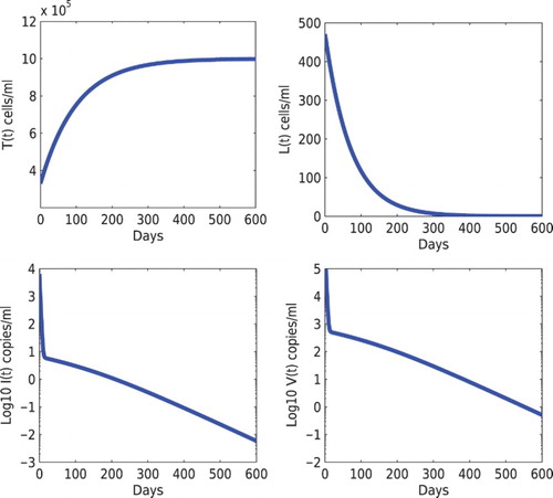
Using these parameters, the basic reproductive number was calculated to be $R_0=3.0>1$. By Theorems 2.3 and 4.2, the infected steady-state $E^{\ast }=(3.3\times {10}^5,471,6.5\times {10}^3,5.7\times {10}^5)$ is locally and also globally asymptotically stable (Figure 1). Under treatment that reduces the infection rates, we assumed the infection rates to be $\beta =2.4\times {10}^{-10}\mathrm{cells}{\mathrm{ml}}^{-1}{\mathrm{day}}^{-1}$ and $k=8\times {10}^{-7}\mathrm{cells}{\mathrm{ml}}^{-1}{\mathrm{day}}^{-1}$. The effective reproductive number under treatment becomes $R_0=0.8<1$. It follows from Theorems 2.2 and 4.1 that the infection-free steady-state $E_0=(1.0\times {10}^6,0,0,0)$ is locally and globally asymptotically stable. Numerical simulation using the steady state obtained from Figure 1 as the initial condition was shown in Figure 2.

Figure 1. Stability of the infected steady state of model (1(1) $\begin{array}{rl}\frac{\mathrm{d}T\left(t\right)}{\mathrm{d}t}& =s-d_{T}T\left(t\right)-\beta T\left(t\right)V\left(t\right)-kT\left(t\right)I\left(t\right),\\ \frac{\mathrm{d}L\left(t\right)}{\mathrm{d}t}& =f\beta T(t-{\tau }_1)V(t-{\tau }_1){\mathrm{e}}^{-{\delta }_1{\tau }_1}+\eta kT(t-{\tau }_1)I(t-{\tau }_1){\mathrm{e}}^{-{\delta }_1{\tau }_1}\\ & -(\alpha +{\delta }_L)L\left(t\right),\\ \frac{\mathrm{d}I\left(t\right)}{\mathrm{d}t}& =(1-f)\beta T(t-{\tau }_2)V(t-{\tau }_2){\mathrm{e}}^{-{\delta }_1{\tau }_2}+(1-\eta )kT(t-{\tau }_2)I(t-{\tau }_2){\mathrm{e}}^{-{\delta }_1{\tau }_2}\\ & -\delta I\left(t\right)+\alpha L\left(t\right),\\ \frac{\mathrm{d}V\left(t\right)}{\mathrm{d}t}& =N\delta I\left(t\right)-cV\left(t\right),\end{array}$(1) ). The initial condition is $(1.0\times {10}^6,0,0,1.0\times {10}^{-3})$. When the infection rates are chosen to be $\beta =2.4\times {10}^{-8}\mathrm{ml}{\mathrm{day}}^{-1}$ and $k=1\times {10}^{-6}\mathrm{ml}{\mathrm{day}}^{-1}$, the basic reproduction number is $R_0=3.0>1$. The solution converges to the infected steady-state $E^{\ast }=(3.3\times {10}^5,471,6.5\times {10}^3,5.7\times {10}^5)$. The other parameters are given in Section 5.

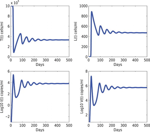
Figure 2. Stability of the infection-free steady state of model (1(1) $\begin{array}{rl}\frac{\mathrm{d}T\left(t\right)}{\mathrm{d}t}& =s-d_{T}T\left(t\right)-\beta T\left(t\right)V\left(t\right)-kT\left(t\right)I\left(t\right),\\ \frac{\mathrm{d}L\left(t\right)}{\mathrm{d}t}& =f\beta T(t-{\tau }_1)V(t-{\tau }_1){\mathrm{e}}^{-{\delta }_1{\tau }_1}+\eta kT(t-{\tau }_1)I(t-{\tau }_1){\mathrm{e}}^{-{\delta }_1{\tau }_1}\\ & -(\alpha +{\delta }_L)L\left(t\right),\\ \frac{\mathrm{d}I\left(t\right)}{\mathrm{d}t}& =(1-f)\beta T(t-{\tau }_2)V(t-{\tau }_2){\mathrm{e}}^{-{\delta }_1{\tau }_2}+(1-\eta )kT(t-{\tau }_2)I(t-{\tau }_2){\mathrm{e}}^{-{\delta }_1{\tau }_2}\\ & -\delta I\left(t\right)+\alpha L\left(t\right),\\ \frac{\mathrm{d}V\left(t\right)}{\mathrm{d}t}& =N\delta I\left(t\right)-cV\left(t\right),\end{array}$(1) ). The initial condition was chosen to be the infected steady state shown in Figure 1. When the infection rates under treatment become $\beta =2.4\times {10}^{-10}\mathrm{ml}{\mathrm{day}}^{-1}$ and $k=8\times {10}^{-7}\mathrm{ml}{\mathrm{day}}^{-1}$, the basic reproduction number is $R_0=0.8<1$. The solution converges to the infection-free steady state $E_0=(1.0\times {10}^6,0,0,1.0\times {10}^{-3})$. The other parameters are given in Section 5.

5.2. Effects of time delays and fractions of infection leading to latency

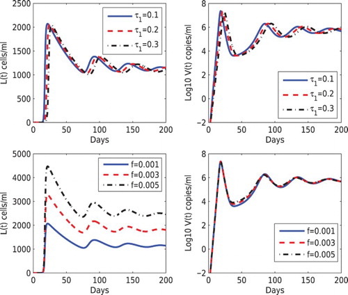
To study the influence of time delays ${\tau }_1,{\tau }_2$ on the dynamics of the latent reservoir and the viral load, we increased ${\tau }_1$ from 0.1 days to 0.3 days but fixed ${\tau }_2=0.5$ days (notice that ${\tau }_2>{\tau }_1$) and other parameter values in the upper panel of Figure 3. As ${\tau }_1$ increases, the time to reach the peak levels of the latent reservoir and the viral load also increases but the magnitude of the peak levels decreases. There is almost no change in the steady states. In the lower panel of Figure 3, we evaluated the influence of the fraction of infection that leads to latency on the dynamics. We fixed the fraction leading to latency via the cell-to-cell transmission ($\eta =0.005$) but increased the latency fraction via the virus-to-cell infection (f) from 0.001 to 0.005. As f increases, the latent reservoir size also increases. However, there is almost no change in the viral load dynamics. This shows that the contribution to the viral replication from latent infection is relatively small.

Figure 3. Effects of different values of the delay $\left({\tau }_1\right)$ and the fraction leading to latency via virus-to-cell infection (f) on the dynamics of latently infected cells and the viral load. Top panel: ${\tau }_1$ was chosen to be 0.1, 0.2, 0.3 days, and ${\tau }_2=0.5$ days was fixed. Bottom panel: f was chosen to be 0.001, 0.003, 0.005, and $\eta =0.005$ was fixed. The other parameter values are the same as those in Figure 1.

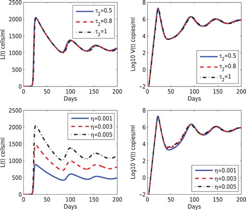
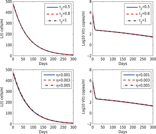
In Figure 4, we performed the simulation using different values of ${\tau }_2$ and η. In the upper panel, we fixed ${\tau }_1=0.25$ days but varied ${\tau }_2$ between 0.5 and 1 days. We found no difference in the latent reservoir and the viral load as ${\tau }_2$ changes. In the lower panel of Figure 4, we increased the fraction that leads to latency via the cell-to-cell transmission ($\eta =0.001$, 0.003, and 0.005) but fixed f=0.001. Similar to the prediction in Figure 3, the latent reservoir increases as η increases but the vial load change is not affected.

Figure 4. Effects of different values of the delay $\left({\tau }_2\right)$ and the fraction leading to latency via cell-to-cell transmission (η) on the dynamics of latently infected cells and the viral load. Top panel: ${\tau }_2$ was chosen to be 0.5, 0.8, 1 days, and ${\tau }_1=0.25$ days was fixed. Bottom panel: η was chosen to be 0.001, 0.003, 0.005, and f=0.001 was fixed. The other parameter values are the same as those in Figure 1.

Figures 3 and 4 showed the sensitivity of modelling prediction to the time delay and latency fraction parameters when the basic reproductive number is greater than 1. In parallel, we conducted simulations with $R_0<1$ using the reduced infection rates β and k as in Figure 2. Figures 5 and 6 showed the simulations with $R_0<1$ using different time delays (${\tau }_1$ and ${\tau }_2$) and different fractions that lead to latent infection (f and η). We found that there is almost no difference in the dynamics of the latent reservoir and the viral load. Therefore, although the time delay and the fraction leading to latency may affect the dynamics during primary infection before treatment, they have no influence on the decay dynamics of the latent reservoir and the viral load under suppressive therapy.

Figure 5. Effects of different values of $\left({\tau }_1\right)$ and f on the dynamics of latently infected cells and the viral load under suppressive therapy. The infection rates β and k are the same as those in Figure 2. The other parameters are the same as those in Figure 3.

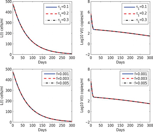
Figure 6. Effects of different values of $\left({\tau }_2\right)$ and η on the dynamics of latently infected cells and the viral load under suppressive therapy. The infection rates β and k are the same as those in Figure 2. The other parameters are the same as those in Figure 4.

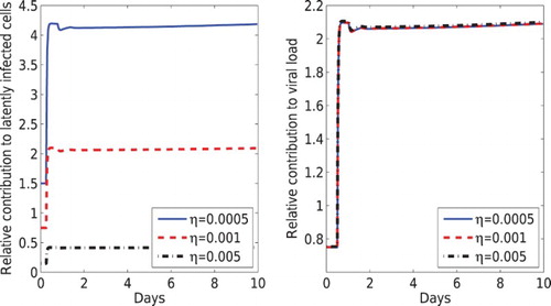
5.3. Relative contribution from the two modes of viral transmission

A critical question is the relative contribution to the latent reservoir and the viral load from the two modes of viral transmission. We used the following fraction $C_L$ to quantify the relative contribution to the latent reservoir from the virus-to-cell and the cell-to-cell viral transmission, and $C_V$ to quantify the relative contribution to the viral load from the two transmission modes: (34) $C_L=\frac{f\beta T(t-{\tau }_1)V(t-{\tau }_1){\mathrm{e}}^{-{\delta }_1{\tau }_1}}{\eta kT(t-{\tau }_1)I(t-{\tau }_1){\mathrm{e}}^{-{\delta }_1{\tau }_1}}$(34) and (35) $C_V=\frac{(1-f)\beta T(t-{\tau }_2)V(t-{\tau }_2){\mathrm{e}}^{-{\delta }_1{\tau }_2}+f\beta T(t-{\tau }_1)V(t-{\tau }_1){\mathrm{e}}^{-{\delta }_1{\tau }_1}\cdot \frac{\alpha }{\alpha +{\delta }_L}}{(1-\eta )kT(t-{\tau }_2)I(t-{\tau }_2)e^{-{\delta }_1{\tau }_2}+\eta kT(t-{\tau }_1)I(t-{\tau }_1){\mathrm{e}}^{-{\delta }_1{\tau }_1}\cdot \frac{\alpha }{\alpha +{\delta }_L}}.$(35) In the expression of $C_V$, the second terms in the numerator and denominator represent the contribution to viral production from the activation of latently infected cells via the virus-to-cell and cell-to-cell transmission, respectively.

Because of the very small fractions (f and η) of infection that lead to latency and the quasi-steady-state assumption (the viral load is proportional to the level of productively infected cells, that is, $V\left(t\right)=N\delta I\left(t\right)/c$), we simplified $C_V$ as $C_V\approx \frac{\beta T(t-{\tau }_2)V(t-{\tau }_2){\mathrm{e}}^{-{\delta }_1{\tau }_2}}{kT(t-{\tau }_2)I(t-{\tau }_2){\mathrm{e}}^{-{\delta }_1{\tau }_2}}\approx \frac{\beta N\delta }{kc}.$ Under the quasi-steady-state assumption, we also had $C_L\approx \frac{f}{\eta }\cdot \frac{\beta N\delta }{kc}.$ Thus, $C_L\approx \frac{f}{\eta }\cdot C_V.$ Recall that $R_{01}=\frac{N\beta s}{c{d}_T}\left(\frac{\alpha f}{\alpha +{\delta }_L}{\mathrm{e}}^{-{\delta }_1{\tau }_1}+(1-f){\mathrm{e}}^{-{\delta }_1{\tau }_2}\right)$ and $R_{02}=\frac{ks}{\delta d_T}\left(\frac{\alpha \eta }{\alpha +{\delta }_L}{\mathrm{e}}^{-{\delta }_1{\tau }_1}+(1-\eta ){\mathrm{e}}^{-{\delta }_1{\tau }_2}\right)$ are the contribution to the basic reproductive number $R_0$ from the virus-to-cell and cell-to-cell transmission, respectively. We called $R_{01}$ the basic reproductive number from the virus-to-cell infection and $R_{02}$ the basic reproductive number from the cell-to-cell viral transmission. Because the fractions f and η are very small, we had $\frac{R_{01}}{R_{02}}\approx \frac{\beta N\delta }{kc}.$ Therefore, we obtained the estimates of the relative contributions to the viral load and the latent reservoir from the two transmission modes (36) $C_V\approx \frac{R_{01}}{R_{02}},C_L\approx \frac{f}{\eta }\cdot \frac{R_{01}}{R_{02}}.$(36)

In Figure 7, we plotted the relative contribution to the latent reservoir and the viral load according to Equations (34) and (35), respectively. We found that the relative contributions agree with the estimates in Equation (36) after a very short time. From the estimates (36), the relative contribution to the viral load from the two transmission modes is the same as the ratio of the two basic reproductive numbers $R_{01}$ and $R_{02}$. The fractions of infection that lead to latency have a negligible effect on the relative contribution to the viral load. However, the relative contribution to the latent reservoir is highly dependent on the fractions that lead to HIV latency via these two modes of viral transmission.

Figure 7. The relative contribution from the virus-to-cell and cell-to-cell transmission to the latent reservoir (left) and to the viral load (right). Different values of the latency fraction η were used (0.005, 0.001 and 0.0005) and f=0.001 was fixed. The other parameter values are the same as those in Figure 1.

6. Conclusion and discussion

Both in vitro and in vivo experiments have showed that HIV can infect cells via two types of strategies: one is the virus-to-cell infection and the other is the cell-to-cell viral transmission [28, 45]. Many existing mathematical models of HIV infection studied virus dynamics with only the virus-to-cell infection. In this paper, we developed a model including both two modes of virus transmission and studied their contributions to the latent reservoir and the viral load. Time delays between viral entry and the establishment of latent infection or virus production were also included in the model. We obtained the basic reproductive number for the model, which consists of two parts: one is the contribution from the virus-to-cell infection and the other is the contribution from the cell-to-cell transmission. Similar to many within-host or between-host virus dynamic models, the basic reproductive number provides a threshold value for determining when the virus is predicted to die out and when the chronic infection is established.

Numerical simulations showed that time delays between viral entry and DNA integration or viral production don't have a significant impact on the virus and the latent reservoir dynamics. Although the fractions of infection that lead to viral latency via the two transmission modes can affect the latent reservoir size during primary and chronic infection, they have a very minor effect on the decay dynamics of the virus and the latent reservoir in patients under suppressive therapy. We also obtained the estimates for the relative contributions from the two transmission modes to the latent reservoir and the viral load. The relative contribution to the viral load is approximately the ratio of the basic reproductive numbers via the two transmission modes (i.e. $R_{01}$/$R_{02}$). The fractions of infection leading to latency have a minor effect on this relative contribution. However, the relative contribution to the latent reservoir depends heavily on these fractions of latency, as well as the ratio of the two basic reproductive numbers.

Our analysis provides a theoretical estimate of the relative contribution to the virus population from the two transmission modes. However, the relative contribution remains unknown because of unknown parameter values. Different estimates of the relative contribution from the two modes to the viral replication have been obtained in the references [18, 19]. Komarova et al. [19] estimated that the two transmission modes contributed approximately equally to the viral population . Sourisseau et al. [50] found that mildly shaking the cell culture can prevent the cell-to-cell infection. Iwami et al. [18] used this experimental method, combined with mathematical model to fit the data, to estimate that the cell-to-cell infection may account for approximately 60% of viral infection. The cell-to-cell transmission was also predicted to shorten the generation time of virus. Whether the shaking condition of cell culture can completely prevent cell-to-cell infection and whether the prediction from the in vitro cell culture can be applied to in vivo studies are unclear. More comparison of these two transmission modes remain to be further investigated.

Antiretroviral therapy was assumed to reduce the infection rates of both transmission strategies. However, the model is sensitive to the treatment effectiveness. Once the drug efficacy is beyond a threshold value (such that the basic reproductive number $R_0$ is less than 1), the infection is predicted to die out. The cell-to-cell transmission can transfer multiple virions to the target cell simultaneously. Thus, antiretroviral drugs may not be effective in blocking the infection of all virions and thus are less effective in inhibiting the cell-to-cell transmission than the virus-to-cell infection [49]. However, some other studies have shown that the cell-to-cell spread of HIV between cells can be effectively blocked by highly active antiretroviral drugs [1, 28, 37, 51]. Extending our model by including multiple infection and considering how the cell-to-cell transmission affects the efficacy of drugs in interfering with the viral replication cycle [11, 20] will improve the understanding of the dynamics of the latent reservoir and the viral load in patients receiving long-term combination therapy.

Disclosure statement

No potential conflict of interest was reported by the authors.

Additional information

Funding

X. Wang is supported by the NSFC [No.11301453] and Nanhu Scholar Program for Young Scholars of XYNU, the Program for Science and Technology Innovation Talents in Universities of Henan Province [17HASTIT011], Postdoctoral Science Foundation of China [2014M562366], Postdoctoral Science Foundation of Shaanxi Province [2014010], the Universities Young Teachers Program of Henan Province [2014GGJS-093]. L. Rong is supported by the NSF grant DMS-1349939.

References

- L.M. Agosto, P. Zhong, J. Munro, and W. Mothes, Highly active antiretroviral therapies are effective against HIV-1 cell-to-cell transmission, PLoS Pathog. 10 (2014), pp. e1003982. doi: 10.1371/journal.ppat.1003982
- A. Alshorman, X. Wang, J. Meyer, and L. Rong, Analysis of HIV models with two time delays, J. Biol. Dyn. (2016), DOI: 10.1080/17513758.2016.1148202.
- R.A. Alvarez, M.I. Barria, and B.K. Chen, Unique features of HIV-1 spread through T cell virological synapses, PLoS Pathog. 10 (2014), pp. e1004513. doi: 10.1371/journal.ppat.1004513
- E. Beretta and Y. Kuang, Geometric stability switch criteria in delay differential systems with delay dependent parameters, SIAM J.Math. Anal. 33 (2002), pp. 1144–1165. doi: 10.1137/S0036141000376086
- J.M. Carr, H. Hocking, P. Li, and C.J. Burrell, Rapid and efficient cell-to-cell transmission of human immunodeficiency virus infection from monocyte-derived macrophages to peripheral blood lymphocytes, Virology 265 (1999), pp. 319–329. doi: 10.1006/viro.1999.0047
- P. Chen, W. Hubner, M. A. Spinelli, and B. K. Chen, Predominant mode of human immunodeficiency virus transfer between T cells is mediated by sustained Env-dependent neutralization-resistant virological synapses, J. Virol. 81 (2007), pp. 12582–12595. doi: 10.1128/JVI.00381-07
- T.-W. Chun, L. Stuyver, S. B. Mizell, L. A. Ehler, J. A. M. Mican, M. Baseler, A. L. Lloyd, M. A. Nowak, and A. S. Fauci, Presence of an inducible HIV-1 latent reservoir during highly active antiretroviral therapy, Proc. Natl. Acad. Sci. 94 (1997), pp. 13193–13197. doi: 10.1073/pnas.94.24.13193
- R.V. Culshaw and S. Ruan, A delay-differential equation model of HIV infection of CD4+ T-cells, Math. Biosci. 165 (2000), pp. 27–39. doi: 10.1016/S0025-5564(00)00006-7
- R.V. Culshaw, S. Ruan, and G. Webb, A mathematical model of cell-to-cell spread of HIV-1 that includes a time delay, J. Math. Biol. 46 (2003), pp. 425–444. doi: 10.1007/s00285-002-0191-5
- O. Diekmann, J.A.P. Heesterbeek, and J.A.J. Metz, On the definition and the computation of the basic reproduction ratio R0 in models for infectious diseases in heterogeneous populations, J. Math. Biol. 28 (1990), pp. 365–382. doi: 10.1007/BF00178324
- N.M. Dixit and A.S. Perelson, Multiplicity of human immunodeficiency virus infections in lymphoid tissue, J. Virol. 78 (2004), pp. 8942–8945. doi: 10.1128/JVI.78.16.8942-8945.2004
- F. Graw and A.S. Perelson, Modeling Viral Spread, Annu. Rev. Virol. (2016), DOI: 10.1146/annurev-virology-110615-042249.
- J.K. Hale and J. Kato, Phase space for retarded equations with infinite delay, Funkcial. Ekvac. 21 (1978), pp. 11–41.
- J.K. Hale and S.M. Verduyn Lunel, Introduction to Functional Differential Equations, Springer Verlag, New York, 1993.
- J.K. Hale and P. Waltman, Persistence in infinite-dimensional systems, SIAM J. Math. Anal. 20 (1989), pp. 388–395. doi: 10.1137/0520025
- G. Huang, Y. Takeuchi, and W. Ma, Lyapunov functionals for delay differential equations model of viral infections, SIAM J. Appl. Math. 70 (2010), pp. 2693–2708. doi: 10.1137/090780821
- W. Hubner, G. P. McNerney, P. Chen, B.M. Dale, R.E. Gordon, F.Y.S. Chuang, X.-. Li, D.M. Asmuth, T. Huser, and B. K. Chen, Quantitative 3D video microscopy of HIV transfer across T cell virological synapses, Science 323 (2009), pp. 1743–1747. doi: 10.1126/science.1167525
- S. Iwami, J. S. Takeuchi, S. Nakaoka, F. Mammano, François Clavel, H. Inaba, T. Kobayashi, N. Misawa, K. Aihara, Y. Koyanagi, and K. Sato, Cell-to-cell infection by HIV contributes over half of virus infection, Elife 4 (2015), pp. e08150. doi: 10.7554/eLife.08150
- N.L. Komarova, D. Anghelina, I. Voznesensky, B. Trinité, D.N. Levy, and D. Wodarz, Relative contribution of free-virus and synaptic transmission to the spread of HIV-1 through target cell populations, Biol. Lett. 9 (2012), DOI: 10.1098/rsbl.2012.1049.
- N.L. Komarova, D.N. Levy, and D. Wodarz, Synaptic transmission and the susceptibility of HIV infection to anti-viral drugs, Sci. Rep. 3 (2013), DOI: 10.1038/srep02103.
- N. L. Komarova, D. N. Levy, D. Wodarz, and A.J. Yates, Effect of synaptic transmission on viral fitness in HIV infection, PLoS One 7 (2012), pp. e48361. doi: 10.1371/journal.pone.0048361
- N.L. Komarova and D. Wodarz, Virus dynamics in the presence of synaptic transmission, Math. Biosci. 242 (2013), pp. 161–171. doi: 10.1016/j.mbs.2013.01.003
- Y. Kuang, Delay Differential Equations: With Applications in Population Dynamics, Academic Press, Boston, 1993.
- X. Lai and X. Zou, Modeling HIV-1 virus dynamics with both virus-to-cell infection and cell-to-cell transmission, SIAM J. Appl. Math. 74 (2014), pp. 898–917. doi: 10.1137/130930145
- X. Lai and X. Zou, Modeling cell-to-cell spread of HIV-1 with logistic target cell growth, J. Math. Anal. Appl. 426 (2015), pp. 563–584. doi: 10.1016/j.jmaa.2014.10.086
- M. Marsh and A. Helenius, Virus entry: Open sesame, Cell 124 (2006), pp. 729–740. doi: 10.1016/j.cell.2006.02.007
- N. Martin and Q. Sattentau, Cell-to-cell HIV-1 spread and its implications for immune evasion, Curr. Opin. HIV AIDS 4 (2009), pp. 143–149. doi: 10.1097/COH.0b013e328322f94a
- N. Martin, S. Welsch, C. Jolly, J.A.G. Briggs, D. Vaux, and Q.J. Sattentau, Virological synapse-mediated spread of human immunodeficiency virus type 1 between T cells is sensitive to entry inhibition, J. Virol. 84 (2010), pp. 3516–3527. doi: 10.1128/JVI.02651-09
- B. Monel, E. Beaumont, D. Vendrame, O. Schwartz, D. Brand, and F. Mammano, HIV cell-to-cell transmission requires the production of infectious virus particles and does not proceed through env-mediated fusion pores, J. Virol. 86 (2012), pp. 3924–3933. doi: 10.1128/JVI.06478-11
- W. Mothes, N. M. Sherer, J. Jin, and P. Zhong, Virus cell-to-cell transmission, J. Virol. 84 (2010), pp. 8360–8368. doi: 10.1128/JVI.00443-10
- M.A. Nowak and C.R.M. Bangham, Population dynamics of immune responses to persistent viruses, Science 272 (1996), pp. 74–79. doi: 10.1126/science.272.5258.74
- P.W. Nelson and A.S. Perelson, Mathematical analysis of delay differential equation models of HIV-1 infection, Math. Biosci. 179 (2002), pp. 73–94. doi: 10.1016/S0025-5564(02)00099-8
- A.S. Perelson, Modelling viral and immune system dynamics, Nat. Rev. Immunol. 2 (2002), pp. 28–36. doi: 10.1038/nri700
- A. S. Perelson, P. Essunger, Y. Cao, M. Vesanen, A. Hurley, K. Saksela, M. Markowitz, and D. D. Ho, Decay characteristics of HIV-1-infected compartments during combination therapy, Nature 387 (1997), pp. 188–191. doi: 10.1038/387188a0
- A.S. Perelson and P.W. Nelson, Mathematical analysis of HIV-1 dynamics in vivo, SIAM Rev. 41 (1999), pp. 3–44. doi: 10.1137/S0036144598335107
- A. S. Perelson, A. U. Neumann, M. Markowitz, J. M. Leonard, and D. D. Ho, HIV-1 dynamics in vivo: Virion clearance rate, infected cell life-span, and viral generation time, Science 271 (1996), pp. 1582–1586. doi: 10.1126/science.271.5255.1582
- M. Permanyer, E. Ballana, A. Ruiz, R. Badia, E. Riveira-Munoz, E. Gonzalo, B. Clotet, and José A. Esté, Antiretroviral agents effectively block HIV replication after cell-to-cell transfer, J. Virol. 86 (2012), pp. 8773–8780. doi: 10.1128/JVI.01044-12
- D.M. Phillips, The role of cell-to-cell transmission in HIV infection, AIDS 8 (1994), pp. 719–732. doi: 10.1097/00002030-199406000-00001
- H. Pourbashash, S. S. Pilyugin, P. D. Leenheer, and C. McCluskey, Global analysis of within host virus models with cell-to-cell viral transmission, Discrete Contin. Dyn. Syst. Ser. B 19 (2014), pp. 3341–3357. doi: 10.3934/dcdsb.2014.19.3341
- L. Rong, Z. Feng, and A.S. Perelson, Mathematical analysis of age-structured HIV-1 dynamics with combination antiretroviral therapy, SIAM J. Appl. Math. 67 (2007), pp. 731–756. doi: 10.1137/060663945
- L. Rong, Z. Feng, and A.S. Perelson, Emergence of HIV-1 drug resistance during antiretroviral treatment, Bull. Math. Biol. 69 (2007), pp. 2027–2060. doi: 10.1007/s11538-007-9203-3
- L. Rong and A.S. Perelson, Modeling HIV persistence, the latent reservoir, and viral blips, J. Theoret. Biol. 260 (2009), pp. 308–331. doi: 10.1016/j.jtbi.2009.06.011
- L. Rong and A.S. Perelson, Modeling latently infected cell activation: Viral and latent reservoir persistence, and viral blips in HIV-infected patients on potent therapy, PLoS Comput. Biol. 5 (2009), pp. e1000533. doi: 10.1371/journal.pcbi.1000533
- L. Rong and A.S. Perelson, Asymmetric division of activated latently infected cells may explain the decay kinetics of the HIV-1 latent reservoir and intermittent viral blips, Math. Biosci. 217 (2009), pp. 77–87. doi: 10.1016/j.mbs.2008.10.006
- Q.J. Sattentau, Avoiding the void: Cell-to-cell spread of human viruses, Nat. Rev. Microbiol. 6 (2008), pp. 815–826. doi: 10.1038/nrmicro1972
- Q.J. Sattentau, Cell-to-cell spread of retroviruses, Viruses 2 (2010), pp. 1306–1321. doi: 10.3390/v2061306
- Q.J. Sattentau, The direct passage of animal viruses between cells, Curr. Opin. Virol. 1 (2011), pp. 396–402. doi: 10.1016/j.coviro.2011.09.004
- N.M. Sherer, M.J. Lehmann, L.F. Jimenez-Soto, C. Horensavitz, M. Pypaert, and W. Mothes, Retroviruses can establish filopodial bridges for efficient cell-to-cell transmission, Nat. Cell Biol. 9 (2007), pp. 310–315. doi: 10.1038/ncb1544
- A. Sigal, J.T. Kim, A.B. Balazs, E. Dekel, A. Mayo, R. Milo, and D. Baltimore, Cell-to-cell spread of HIV permits ongoing replication despite antiretroviral therapy, Nature 477 (2011), pp. 95–98. doi: 10.1038/nature10347
- M. Sourisseau, N. Sol-Foulon, F. Porrot, F. Blanchet, and O. Schwartz, Inefficient human immunodeficiency virus replication in mobile lymphocytes, J. Virol. 81 (2007), pp. 1000–1012. doi: 10.1128/JVI.01629-06
- B.K. Titanji, M. Aasa-Chapman, D. Pillay, and C. Jolly, Protease inhibitors effectively block cell-to-cell spread of HIV-1 between T cells, Retrovirology 10 (2013), doi: 10.1186/1742-4690-10-161.
- P. van den Driessche and J. Watmough, Reproduction numbers and sub-threshold endemic equilibria for compartmental models of disease transmission, Math. Biosci. 180 (2002), pp. 29–48. doi: 10.1016/S0025-5564(02)00108-6
- X. Wang, A. Elaiw, and X. Song, Global properties of a delayed HIV infection model with CTL immune response, Appl. Math. Comput. 218 (2012), pp. 9405–9414.
- X. Wang, X. Song, S. Tang, and L. Rong, Dynamics of an HIV model with multiple infection stages and treatment with different drug classes, Bull. Math. Biol. 78 (2016), pp. 1–28. doi: 10.1007/s11538-015-0134-0
- X. Wang, Y. Tao, and X. Song, A delayed HIV-1 infection model with Beddington-DeAngelis functional response, Nonlinear Dyn. 62 (2010), pp. 67–72. doi: 10.1007/s11071-010-9699-1
- J. K. Wong, M. Hezareh, H.F. Gunthard, D.V. Havlir, C.C. Ignacio, C.A. Spina, and D.D. Richman, Recovery of replication-competent HIV despite prolonged suppression of plasma viremia, Science 278 (1997), pp. 1291–1295. doi: 10.1126/science.278.5341.1291
- A. Yakimovich, H. Gumpert, C.J. Burckhardt, V.A. Lutschg, A. Jurgeit, I.F. Sbalzarini, and U.F. Greber, Cell-free transmission of human adenovirus by passive mass transfer in cell culture simulated in a computer model, J. Virol. 86 (2012), pp. 10123–10137. doi: 10.1128/JVI.01102-12
- Y. Yang, L. Zou, and S. Ruan, Global dynamics of a delayed within-host viral infection model with both virus-to-cell and cell-to-cell transmissions, Math. Biosci. 270 (2015), pp. 183–191. doi: 10.1016/j.mbs.2015.05.001
- P. Zhong, L. M. Agosto, A. Ilinskaya, B. Dorjbal, R. Truong, D. Derse, P. D. Uchil, G. Heidecker, W. Mothes, and F. Mammano, Cell-to-cell transmission can overcome multiple donor and target cell barriers imposed on cell-free HIV, PLoS One 8 (2013), pp. e53138. doi: 10.1371/journal.pone.0053138
- P. Zhong, L. M. Agosto, J. B. Munro, and W. Mothes, Cell-to-cell transmission of viruses, Curr. Opin. Virol. 3 (2013), pp. 44–50. doi: 10.1016/j.coviro.2012.11.004