
 ?Mathematical formulae have been encoded as MathML and are displayed in this HTML version using MathJax in order to improve their display. Uncheck the box to turn MathJax off. This feature requires Javascript. Click on a formula to zoom.
ABSTRACT
Oscillators are essential to fuel autonomous behaviours in molecular systems. Artificial oscillators built with programmable biological molecules such as DNA and RNA are generally easy to build and tune, and can serve as timers for biological computation and regulation. We describe a new artificial nucleic acid biochemical reaction network, and we demonstrate its capacity to exhibit oscillatory solutions. This network can be built in vitro using nucleic acids and three bacteriophage enzymes, and has the potential to be implemented in cells. Numerical simulations suggest that oscillations occur in a realistic range of reaction rates and concentrations.
1. Introduction
All organisms require timing circuits to orchestrate processes related to their life cycle, such as cell growth, metabolism, and division [Citation36]. By building molecular timers from the bottom up, we have an opportunity to understand the design requirements to programme periodic biochemical behaviours. In addition, synthetic oscillators are useful components to direct autonomous molecular operations in vivo and in vitro [Citation11,Citation13,Citation30,Citation33,Citation35].
In vitro nucleic acid oscillators can be built with a small number of parts, and their behaviour is quantitatively predictable [Citation15,Citation16,Citation19,Citation22,Citation35]. Nucleic acids have become molecular building blocks for a variety of logic and dynamic circuits, because their thermodynamic and kinetic interactions can be programmed by choosing their sequence content with rational optimization algorithms. Existing nucleic acid oscillators however cannot be ported to the cellular environment, because they rely on the presence of multiple single-stranded or partially single-stranded DNA species, which are incompatible with the cellular machinery [Citation15,Citation16,Citation19,Citation22]. Here we describe a new nucleic acid oscillator architecture that has the potential to overcome this limitation, as it does not require single-stranded DNA molecules. A particularly interesting aspect of our circuit is that all regulatory interactions are non-cooperative. Therefore, the corresponding model does not include Hill-type nonlinearities, present in the majority of models for molecular non-equilibrium circuits.
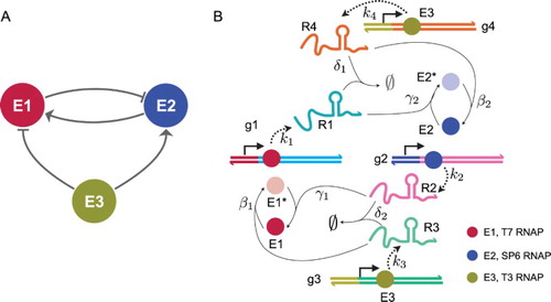
Our oscillator comprises three polymerases, two of which mutually regulate each other (Figure (a )). The interactions among enzymes are defined by four synthetic genes and four RNA species (Figure (b )). The activity of two of the enzymes is modulated by RNA species that serve as inhibitors or activators. The third enzyme species controls the baseline production of two of the RNA species, and has a net effect of counteracting the mutual regulation of the other two enzymes. For instance, let us consider the pathway by which enzyme is inhibited by enzyme
and activated by enzyme
.
produces RNA species
by transcribing gene
;
binds to and inhibits enzyme
, converting it to inactive enzyme
(a reaction experimentally demonstrated, for instance, in [Citation23, Citation24]). RNA species
(transcribed by
) counteracts this pathway and causes reactivation of
(conversion of
to
), because it is designed to displace
bound to
, and to titrate free
as well. Similar reactions generate inhibition and activation pathways for
(due to
and to
, respectively). Overall, these interactions contribute to creating a negative feedback loop. This system can be experimentally implemented using T7, T3, and SP6 bacteriophage RNA polymerases [Citation20,Citation21,Citation31], which can be purchased off-the-shelf from many vendors. RNA sequences (known as aptamers [Citation12]) that bind to bacteriophage RNA polymerases and work as inhibitors have been experimentally characterized [Citation23,Citation24]. RNA activators can be designed as strands whose sequences are complementary to the sequences of the inhibitors via the mechanism of strand displacement and strand titration [Citation18,Citation37].
Figure 1. (a) Architecture of the three-node oscillator: enzymes and
mutually regulate their concentration (arrows indicate activation, flat arrows indicate repression) generating a negative feedback loop; enzyme
counteracts the loop regulation.(b) Schematic of the chemical reactions underlying the oscillator architecture. Different enzyme species are indicated as circles of different colour ; bright colour indicates active enzyme, and dim colour indicates inactive enzyme. RNA species are transcribed (dashed arrows) from synthetic genes present at constant concentration; enzymes are activated or inhibited by a given RNA species according to the illustrated reactions and corresponding rates. The full set of reactions is listed in Section 2, and result in ODE systems (Equation1
(1)
(1) ) and (Equation2
(2)
(2) ).
We describe this system by means of ordinary differential equations (ODEs) built using the law of mass action, starting from a list of chemical reactions reported in Section 2. We demonstrate that the system is a candidate oscillator due to the sign pattern of its Jacobian matrix [Citation4, Citation5]; in particular we show that the system admits transitions to instability that are exclusively oscillatory.
Our analysis relies on monotone systems theory (background is provided in Section 3) and the theory of invariant sets. In Section 4 we study the capacity of this dynamical system to structurally exhibit sustained oscillations whenever it becomes unstable, in view of its particular Jacobian structure; this approach can be applied to a variety of chemical reaction networks, as we have shown, for instance, in the context of other titration-based regulatory networks [Citation9]. Structural (namely, parameter-free) results can greatly help unravel the functioning of biological systems, which are affected by intrinsic uncertainties and variabilities in their parameters, but can nonetheless exhibit an extraordinary robustness and resilience [Citation3]. We conclude with a numerical bifurcation analysis and study of period and amplitude as a function of variations in individual parameters, showing that for realistic reaction rates the system exhibits oscillatory behaviours (Section 5). We previously described a two-enzyme oscillator relying on RNA aptamers [Citation2,Citation10]; we claim that a three-enzyme system is more tunable, and simulation results indicate that in a certain region of parameter space its amplitude can be modulated independently of the period.
2. A three-enzyme oscillator regulated by first- and second-order reactions
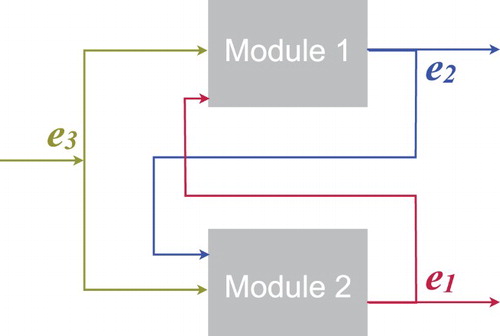
In the following, capital letters represent chemical species and the corresponding lowercase letters represent species concentrations (e.g. species A has concentration a). Our three-node oscillator is described by the biochemical reactions below. Reactions are grouped in two sets corresponding to functional modules (Figure ), whose common external input is . For simplicity we assume a common degradation rate for all products
.
Figure 2. Schematic of the interconnections between reaction Modules 1 and 2, with enzyme concentrations as inputs and outputs.
The differential equations describing Module 1 are:
(1)
(1)
The differential equations describing Module 2 are:
(2)
(2)
The total concentration of and
is assumed to be constant, and equal to
and
, respectively; hence, mass conservation laws yield
and
. The two modules are interconnected and form a feedback loop: Module 1 (associated with variables
,
and
) receives input
from Module 2; in turn, Module 2 (associated with variables
,
and
) receives input
from Module 1. Both modules receive input
, which we assume is constant (Figure ); we assume that the timescale at which
binds to a gene and transcribes RNA is fast relative to the other timescales in the system, so that its dynamics can be neglected; this assumption is sensible for short transcripts (30–60 bases). In the next sections we demonstrate that transitions to instability in this system can occur exclusively due to a pair of complex conjugate eigenvalues crossing the imaginary axis, hence sustained oscillations necessarily arise whenever the system is driven to instability. From numerical simulations it is apparent that the system can actually be destabilized, for suitable parameter choices, and is therefore a good candidate oscillator.
3. Background
We summarize several background notions that are required to introduce our main results in Section 4. Additional information can be found in references [Citation4,Citation5]. Consider a system:
(3)
(3) where μ is a real-valued parameter and
is a sufficiently smooth function, continuous in μ, satisfying the following Assumptions for every admissible value of μ.
Assumption 1.
All the solutions of (Equation3(3)
(3) ) are globally uniformly asymptotically bounded in the compact set
.
Hence, system (Equation3(3)
(3) ) admits an equilibrium
in
[Citation25,Citation26,Citation29].
Assumption 2.
is either always positive, always negative, or always null in the considered domain.
Assumption 3.
For all i, that is, the system is non-autocatalytic.
Due to the monotonicity of with respect to each argument
, the Jacobian matrix
of system (Equation3
(3)
(3) ) is sign definite.
Definition 3.1.
Given a system with a sign-definite Jacobian , its structure is the sign pattern matrix
.
The structure Σ of system (Equation3(3)
(3) ) is assumed to be invariant with respect to μ. Assumption 1 ensures that an equilibrium exists; all the following definitions refer to this equilibrium, which is, in general, a function of μ:
. We assume that
depends continuously on μ. Note that a suitable change of coordinates always allows us to shift the equilibrium to the origin, without affecting our analysis.
Definition 3.2.
System (Equation3(3)
(3) ) undergoes a transition to instability
TI
at
iff its Jacobian matrix
is asymptotically stable in a left neighbourhood of
, and unstable in a right neighbourhood.Footnote1 A TI is simple if at most a single real eigenvalue or a single pair of complex conjugate eigenvalues crosses the imaginary axis.
Definition 3.3.
System (Equation3(3)
(3) ) undergoes an oscillatory transition to instability
OTI
at
iff its Jacobian matrix
has a single pair of pure imaginary eigenvalues, while all the other eigenvalues have negative real part:
with
for k>2 and
for k=1,2 in a right neighbourhood of
.
We now provide general definitions for candidate oscillatory and multistationary systems. We consider system (Equation3(3)
(3) ), with its given structure Σ (invariant with respect to μ), under Assumptions 1, 2 and 3.
Definition 3.4.
A system of the form (Equation3(3)
(3) ), with structure Σ, is structurally a candidate
oscillator in the weak sense iff it admits an OTI for some
;
oscillator in the strong sense iff every simple TI (if any) is an OTI;
Necessary and sufficient conditions characterizing strong and weak oscillators/ multistationary systems are provided in [Citation4] in terms of cycles in the structure graph. We associate matrix Σ with a directed n-node graph, whose arcs are positive (), negative (
), or zero depending on the sign of the corresponding matrix entries.
Definition 3.5.
Given a graph, a cycle is an oriented, closed sequence of distinct nodes connected by distinct directed arcs. A cycle is negative (positive) if the number of negative arcs is odd (even). The order of a cycle is the number of arcs involved in the cycle. We say a system is critical when all negative cycles (if any) are of order two.
Proposition 3.6.
A non-critical system is a candidate oscillator in the weak sense if and only if its structure has at least one negative cycle necessarily of order greater than two
.
Proposition 3.7.
A non-critical system is a candidate oscillator in the strong sense if and only if its structure has only negative cycles.
Proofs for Propositions 3.6 and 3.7 can be found in [Citation4].
Remark 1.
The results above are verified as well if we drop Assumption 1 and we restrict our analysis to solutions that belong to a compact positively invariant set , with a non-empty interior and with no equilibrium points on the boundary.
The graph-based results in [Citation4] have been generalized in [Citation5] to the case of systems that are the sign definite interconnection of subsystems that are either monotone or anti-monotone (as in the case of our system). We provide below the definitions of monotone and anti-monotone system.
Definition 3.8.
A system
(4)
(4) where
is a scalar, time varying input, is input-to-state monotone if, denoting as
and
the solutions of the system corresponding to inputs
and
, the fact that
and
for t>0 implies that
for t>0, where inequalities are intended to hold componentwise. The system is input-to-state anti-monotone if the input has the opposite effect on the state, that is, if
and
for t>0, then
for t>0. If the system includes an output
, the system is input–output monotone (anti-monotone) if it is input-to-state monotone (anti-monotone) and if
implies
A simple characterization of input-to-state monotonicity and anti-monotonicity [Citation1, Citation28] can be provided by exploiting the concept of Metzler matrix: a matrix is Metzler if its elements satisfy ,
such that
.
Theorem 3.9.
System (Equation4(4)
(4) ) is input-to-state monotone if its Jacobian matrix
is a Metzler matrix and
componentwise. Conversely, system
is input-to-state anti-monotone if its Jacobian matrix
is a Metzler matrix and
componentwise.
A more general concept, which we will use in the following, is given by monotonicity (or anti-monotonicity) with respect to a given signature tuple , where
or
for all i [Citation14]: this amounts to requiring that, after changing the sign of the state variables as
for all i, the system becomes monotone (or anti-monotone). Hence, Theorem 3.9 applies to the system in the new coordinates.
4. Analytical results
4.1. Existence of equilibria
First, we show that this system always admits a steady state (equilibrium).
Proposition 4.1.
Consider the interconnection of systems (Equation1(1)
(1) ) and (Equation2
(2)
(2) ). For any constant
there exists a suitably large
such that the compact set
is positively invariant. Moreover, all of the solutions of the system are globally uniformly asymptotically bounded in
hence the interconnection of systems
and
satisfies Assumption 1.
Proof.
The inequalities and
are always satisfied by construction. Consider the constraint
and assume that at some point
. Then
for ρ large enough:
. Hence, the constraint
cannot be violated. Analogously, the constraint
cannot be violated because, if at some point
, then
for
. Then, any value
ensures that
is positively invariant. Also, since
is negative whenever
and
is negative whenever
, any trajectory of the system is uniformly asymptotically bounded in
(indeed,
and
can be taken as Lyapunov-like functions for modules 1 and 2, respectively, to show that all the trajectories of the system are uniformly ultimately bounded in the compact set
[Citation6]).
Proposition 4.2.
The dynamical system defined by the interconnection of systems (Equation1(1)
(1) ) and (Equation2
(2)
(2) ) always admits the existence of a steady-state.
Proof.
The existence of the compact invariant set where the solutions of the system are globally uniformly asymptotically bounded (Proposition 4.1) implies the existence of a steady-state [Citation25,Citation26,Citation29].
We later demonstrate that this steady state is unique.
Remark 2.
The presence of degradation reactions (at rate ) is essential to have structural boundedness. In fact, if we set
and we consider the function
, we have
which may grow unbounded for a large value of
.
4.2. Monotonicity properties and uniqueness of equilibrium point
Now we show that the overall system is the feedback interconnection of two subsystem, corresponding to the modules defined earlier, that are, respectively, anti-monotone and monotone. This property further implies that the system admits a unique equilibrium.
We individually linearize subsystems (Equation1(1)
(1) ) and (Equation2
(2)
(2) ) around an equilibrium point (which is guaranteed to exist), and we begin by studying each subsystem in isolation.
(6)
(6)
(6)
(6)
where the linearized state variables of each subsystems are
and
. We denote equilibrium values of each variable with a
symbol (e.g.
is the equilibrium of
). The linearized dynamics are defined by matrices:
and
The two linearized subsystems are stable, and the matrices defining their dynamics (Jacobian matrices of the nonlinear systems) are Metzler up to changes in the sign of some variables. This can be easily shown by changing sign to the first component of z and to the second component of w:
and
. This is equivalent to changing sign to
and
, where
and
are variables of the original system, and provides matrices:
(7)
(7) and
(8)
(8)
Remark 3.
We have applied a local change of variables, since and
are variables of the linearized system. This is equivalent to applying the linear transformations
and
, with
and
. This leads to the transformed state matrices
and
, and to the transformed input matrices
and
.
Proposition 4.3.
Matrices in Equation
and
in Equation
are Metzler and are Hurwitz stable. Moreover, their inverse matrices are
element-wise
negative.
Proof.
Consider systems (Equation5(6)
(6) ) and (Equation6
(6)
(6) ), which after the sign change have matrices (Equation7
(6)
(6) ) and (Equation8
(7)
(7) ). Since all of their off-diagonal entries are non-negative,
and
are Metzler matrices. They are also irreducible.Footnote2 Hurwitz stability (all the eigenvalues of the Jacobian
have a negative real part) immediately follows from the fact that
and
are Metzler and diagonally dominant, with negative diagonal entries (this is a consequence of Gershgorin's circle theorem). Finally, any stable and irreducible Metzler matrix has an element-wise negative inverse (see [Citation6] for details).
We are now ready to demonstrate the monotonicity properties of the two nonlinear modules.
Proposition 4.4.
Systems and
are, respectively, input-to-state anti-monotone and monotone after the sign change in the relative variables:
(9)
(9)
Proof.
This follows from Theorem 3.9, since the state matrices and
are Metzler, while the input matrices
and
are, respectively, non-positive and non-negative.
Monotonicity and stability have important consequences on the static input-state and input–output characteristics (input–output equilibrium conditions) and on uniqueness of the equilibrium point. Indeed, the feedback of two systems that are either monotone or anti-monotone always admits a single equilibrium point (if any).
We have shown in Proposition 4.2 that an equilibrium always exists; we prove below, for completeness, that the static input–output characteristics of the two modules are monotonic, hence such an equilibrium point is unique.
Proposition 4.5.
We assume that inputs and
in systems
and
are constant. Then, the steady-state values of the modules,
and
depend monotonically on the inputs. Precisely,
and
monotonically increase as a function of
while
and
monotonically decrease as a function of
.
Proof.
We recall that, for a generic system , the steady-state characteristic
is implicitly defined by
We can apply the implicit function theorem to find its derivative:
Consider Module 1, after the sign change in the variables in Equation (Equation9
(8)
(8) ):
The inequality holds componentwise (Proposition 4.3), hence after the sign change equilibria
,
and
are monotonically decreasing functions of
.
As for Module 2, after the sign change in Equation (Equation9(8)
(8) ):
componentwise, hence after the sign change
,
and
are monotonically increasing functions of input
.
Proposition 4.6.
The interconnection of systems (Equation1(1)
(1) ) and (Equation2
(2)
(2) ) admits a unique equilibrium.
Proof.
The system always admits a steady state, as shown in Proposition 4.2. Due to Proposition 4.5, is a decreasing function and
is an increasing function. Thus, the system of equations:
has a unique solution.
It is possible to demonstrate that this unique equilibrium is strictly positive, and there cannot be equilibria with zero components. This claim can be proved by showing that the two equilibrium equations intersect for positive values of and
. Then, we can show that all other variables have a positive steady-state from their equilibrium conditions, which are all derived analytically in the appendix.
4.3. The interconnected system admits exclusively oscillatory transitions to instability
Based on the properties demonstrated in the previous sections, we establish that our three-enzyme network has the appropriate structure to exhibit sustained oscillations, whenever it is driven to instability. More precisely, the network admits exclusively oscillatory transitions to instability.
Proposition 4.7.
The interconnection of systems and
is a strong candidate oscillator.
Proof.
The Jacobian of the overall system, with variables ordered as (,
,
,
,
,
) and with the variable sign change
and
, highlights that the system is the negative feedback interconnection of two monotone subsystems:
 Due to Proposition 4.1, the system satisfies Assumption 1. By inspecting the Jacobian matrix, it is apparent that Assumptions 2 and 3 are also satisfied. Therefore, the system is a strong candidate oscillator [Citation4,Citation5]. This means that the system can transition to instability exclusively due to a pair of complex conjugate eigenvalues crossing the imaginary axis (OTI) and yielding oscillatory dynamics.
5. Numerical analysis
Model (Equation1(1)
(1) )–(Equation2
(2)
(2) ) was integrated using the MATLAB routine ode23. Bifurcation analysis, period and amplitude computation was also done writing MATLAB scripts ad hoc.
In the numerical analysis that follows, we choose nominal parameters (Table ) that are compatible with reaction rates measured in nucleic acid strand displacement reactions and in vitro transcription. An example solution trajectory for Model (Equation1(1)
(1) )–(Equation2
(2)
(2) ), integrated with the nominal parameters, is shown in Figure .
Figure 3. Left: Time evolution of and
when parameters are chosen as in Table . Right: Trajectories in the plane
–
(black) and equilibrium conditions (red and blue).
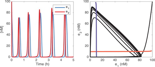
Table 1. Nominal simulation parameters.
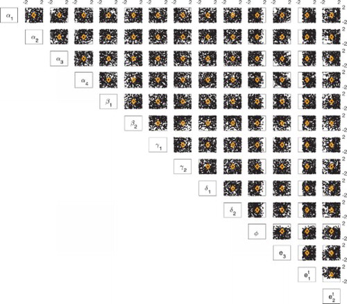
5.1. Randomized parameter sampling
First, we selected random values for the parameters sampling from a uniform distribution in the interval to
times the nominal parameter value (Table ). We locate peaks and wells of the oscillations and compute period and amplitude as averaged over all the measured peaks and wells. A trajectory is classified as oscillatory if at least three oscillations are measured, if the period of the trajectory is between 0.5 and 40 h, and its amplitude is larger than 1 nM. This plot highlights that high degradation rates and low concentrations of
and
are associated with loss of oscillations ().
Figure 4. We randomly choose parameters in the interval to
times their nominal value (listed in Table ). Each black dot in this plot indicates that the (randomly) chosen parameter vector results in oscillations. Axes are in log scale. Orange diamonds represent the nominal value of each parameter (Table ).
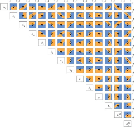
5.2. Bifurcation analysis
Using analytical equilibrium conditions (expressions (EquationA.1(A.1)
(A.1) ) and (EquationA.2
(A.2)
(A.2) ) reported in the appendix), we find equilibria numerically and compute the eigenvalues of Jacobian (Equation10
(A.1)
(A.1) ) at the equilibria. If at least one pair of complex conjugate eigenvalues with non-negative real part is found, the equilibrium is classified as oscillatory. We vary two parameters simultaneously, while all others are kept constant as in Table . Oscillatory regions are shown in orange in Figure , while stable regions are shown in blue.
Figure 5. Log plots showing how varying pairs of parameters influences the stability of the equilibrium. Each parameter was varied between one tenth to 10 times its nominal value (black diamond; nominal values listed in Table ). Orange regions indicate oscillatory behaviour; blue regions indicate a single stable equilibrium.
5.3. Period and amplitude
We focus on the influence of reaction rates and total concentrations of on the period and amplitude. Parameters
,
,
,
,
,
and
are particularly relevant because they are experimentally easy to change (Figure(b)):
,
, are transcription rates, which can be tuned by mutating the promoter region;
,
and
can be chosen by the experimenter.
We compute the period and amplitude from integrated solutions to the ODEs. As explained in Section 5.1, we locate peaks and wells of the oscillations and compute period and amplitude as averaged over all the measured peaks and wells. A trajectory is classified as oscillatory if its period is between 0.5 and 40 h, and its amplitude is larger than 1 nM. The results are shown in Figures and , where each individual parameter is varied in the range of one tenth to 10 times its nominal value, while other parameters are held fixed at their nominal value (Table ). Correlation between period and amplitude is shown in Figure . To discriminate between damped and sustained oscillations, we check the sign of the real part of complex conjugate eigenvalues of the Jacobian matrix (evaluated at the considered combination of parameters). In Figures –, damped oscillations are marked by blue circles, and sustained oscillations are marked by red circles.
Figure 6. Period (h) as a function of each parameter (x axis in log scale). The period was computed numerically for damped and sustained oscillations. We classify a solution as oscillatory (damped or sustained) as long as the period is between 0.5 and 40 h, and the amplitude is larger than 1 nM. Blue circles indicate when the Jacobian has at least one pair of complex eigenvalues with negative real part (damped oscillations). Red circles indicate when the Jacobian has at least one pair of complex eigenvalues with positive real part (sustained oscillations). The parameters were changed in the range of one tenth to 10 times their nominal values.
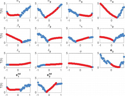
Figure 7. Amplitude (nM) as a function of each parameter (x axis in log scale). We computed numerically the amplitude of the solutions, as long as they classify as damped or sustained oscillations (period between 0.5 and 40 h and amplitude larger than 1 nM). Blue circles indicate when the Jacobian has at least one pair of complex eigenvalues with negative real part (damped oscillations). Red circles indicate when the Jacobian has at least one pair of complex eigenvalue with positive real part (sustained oscillations). The parameters were changed in the range of one tenth to 10 times their nominal values.
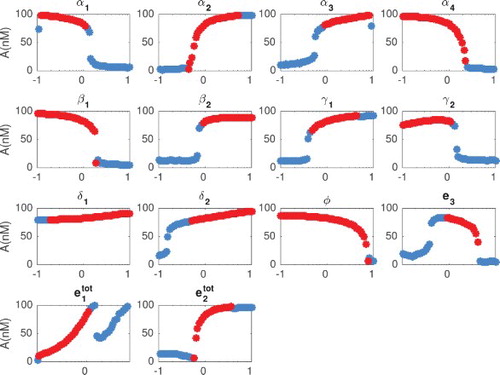
Figure 8. Period (h) and amplitude (nM) correlation. This figure combines the results plotted in Figures and . Amplitude and period of the solutions were computed numerically for both damped and sustained oscillations (period between 0.5 and 40 h and amplitude larger than 1 nM). Blue circles indicate when the Jacobian has at least one pair of complex eigenvalues with negative real part (damped oscillations). Red circles indicate when the Jacobian has at least one pair of complex eigenvalues with positive real part (sustained oscillations). Parameters were changed in the range of 0.1–10 times their nominal values.
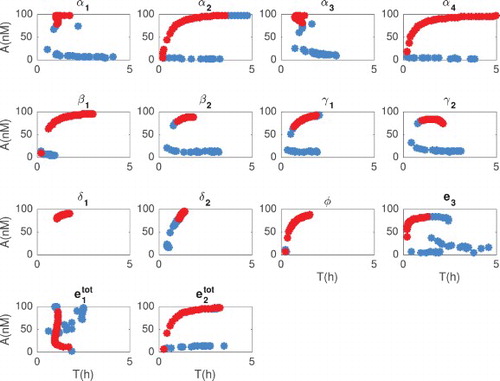
From Figures and we observe that the period can be tuned from 0 to 5 hours. Also, the parameters related to the kinetics rate can change the period up to 3 hours in the range of one tenth to 10 times their nominal value.
These plots show that when varying in a range between 0.1 and 10 times its nominal value, the period remains flat. In that same range, amplitude varies significantly. We also observe that varying
between 0.1 and 10 times its nominal value, amplitudes stays flat while the period varies between 0 and 3 h. It is worth noting that the titration rates
and
do not affect drastically neither amplitude nor period, which indicates that the system performance is robust relative to variations in the titration rates.
We observe that there is a range in which parameters and
could be varied to tune exclusively the period, while the amplitude remains nearly constant. Alternatively, there is a range in which parameters
and
could be varied to modulate exclusively the amplitude, keeping the period nearly unchanged (and slow).
6. Conclusion
We have described an artificial three-enzyme biochemical network that has the capacity to oscillate. The network is designed for in vitro implementation with nucleic acid components and bacteriophage RNA polymerases, but has the potential to be implemented in vivo as well. The polymerases transcribe synthetic genes whose RNA transcripts in turn regulate enzyme activity, generating a negative feedback loop that is necessary for oscillations (the famous Thomas' conjecture [Citation27,Citation32]). We analytically demonstrate that this architecture can exclusively undergo oscillatory transitions to instability, due to the structure of its Jacobian matrix. Numerical analysis shows that in a range of realistic parameters the system oscillates; simulations are useful to direct the experimental implementation of this circuit, which is currently being pursued.
Disclosure statement
No potential conflict of interest was reported by the authors.
Additional information
Funding
Notes
1 The definition holds as well for systems transitioning to instability from the right to the left neighbourhood of : just take
as the bifurcation parameter.
2 A matrix is irreducible if there does not exist a permutation of its rows or columns that transforms it into a block triangular matrix.
References
- D. Angeli and E. Sontag, Monotone control systems, IEEE Trans. Automat. Control 48 (2003), pp. 1684–1698. doi: 10.1109/TAC.2003.817920
- F. Blanchini, C. Cuba Samaniego, E. Franco, and G. Giordano, Design of a molecular clock with RNA-mediated regulation, Proceedings of the IEEE Conference on Decision and Control, 2014, pp. 4611–4616.
- F. Blanchini and E. Franco, Structurally robust biological networks, BMC Syst. Biol. 5 (2011), p. 74. doi: 10.1186/1752-0509-5-74
- F. Blanchini, E. Franco, and G. Giordano, A structural classification of candidate oscillatory and multistationary biochemical systems, Bull. Math. Biol. 76 (2014), pp. 2542–2569. doi: 10.1007/s11538-014-0023-y
- F. Blanchini, E. Franco, and G. Giordano, Structural conditions for oscillations and multistationarity in aggregate monotone systems, Proceedings of the IEEE Conference on Decision and Control, Osaka, Japan, 2015, pp. 609–614.
- F. Blanchini and S. Miani, Set-Theoretic Methods in Control, Systems & Control: Foundations & Applications, Birkhäuser, Basel, 2015.
- N.E. Buchler and M. Louis, Molecular titration and ultrasensitivity in regulatory networks, J. Mol. Biol. 384 (2008), pp. 1106–1119. doi: 10.1016/j.jmb.2008.09.079
- H. Chen, K. Shiroguchi, H. Ge, and X.S. Xie, Genome-wide study of mRNA degradation and transcript elongation in Escherichia coli, Mol. Syst. Biol. 11 (2015), p. 781. doi: 10.15252/msb.20145794
- C. Cuba Samaniego, G. Giordano, J. Kim, F. Blanchini, and E. Franco, Molecular titration promotes oscillations and bistability in minimal network models with monomeric regulators, ACS Synth. Biol. 5 (2016), pp. 321–333. doi: 10.1021/acssynbio.5b00176
- C. Cuba Samaniego, S. Kitada, and E. Franco, Design and analysis of a synthetic aptamer-based oscillator, in American Control Conference (ACC), 2015, 2015, pp. 2655–2660.
- T. Danino, O. Mondragon-Palomino, L. Tsimring, and J. Hasty, A synchronized quorum of genetic clocks, Nature 463 (2010), pp. 326–330. doi: 10.1038/nature08753
- A.D. Ellington and J.W. Szostak, In vitro selection of RNA molecules that bind specific ligands, Nature 346 (1990), pp. 818–822. doi: 10.1038/346818a0
- M.B. Elowitz and S. Leibler, A synthetic oscillatory network of transcriptional regulators, Nature 403 (2000), pp. 335–338. doi: 10.1038/35002125
- G.A. Enciso, Monotone input/output systems, and applications to biological systems, Ph.D. thesis, Graduate School – New Brunswick, Rutgers, The State University of New Jersey, 2005.
- E. Franco, E. Friedrichs, J. Kim, R. Jungmann, R. Murray, E. Winfree, and F.C. Simmel, Timing molecular motion and production with a synthetic transcriptional clock, Proc. Natl. Acad. Sci. 108 (2011), pp. E784–E793. doi: 10.1073/pnas.1100060108
- T. Fujii and Y. Rondelez, Predator–prey molecular ecosystems, ACS nano 7 (2012), pp. 27–34. doi: 10.1021/nn3043572
- J. Kim and R.M. Murray, Analysis and design of a synthetic transcriptional network for exact adaptation, in Biomedical Circuits and Systems Conference (BioCAS), 2011, pp. 345–348.
- J. Kim, K.S. White, and E. Winfree, Construction of an in vitro bistable circuit from synthetic transcriptional switches, Mol. Syst. Biol. 2 (2006), p. 68. doi: 10.1038/msb4100099
- J. Kim and E. Winfree, Synthetic in vitro transcriptional oscillators, Mol. Syst. Biol. 7 (2011), p. 465. doi: 10.1038/msb.2010.119
- P.A. Krieg and D. Melton, In vitro RNA synthesis with SP6 RNA polymerase, Methods Enzymol. 155 (1987), pp. 397–415. doi: 10.1016/0076-6879(87)55027-3
- W.T. McAllister, H. Küpper, and E.K. Bautz, Kinetics of transcription by the bacteriophage-T3 RNA polymerase in vitro, Eur. J. Biochem. 34 (1973), pp. 489–501. doi: 10.1111/j.1432-1033.1973.tb02785.x
- K. Montagne, R. Plasson, Y. Sakai, T. Fujii, and Y. Rondelez, Programming an in vitro DNA oscillator using a molecular networking strategy, Mol. Syst. Biol. 7 (2011), p. 466. doi: 10.1038/msb.2010.120
- Y. Mori, Y. Nakamura, and S. Ohuchi, Inhibitory RNA aptamer against SP6 RNA polymerase, Biochem. Biophys. Res. Commun. 420 (2012), pp. 440–443. doi: 10.1016/j.bbrc.2012.03.014
- S. Ohuchi, Y. Mori, and Y. Nakamura, Evolution of an inhibitory RNA aptamer against T7 RNA polymerase, FEBS Open Bio. 2 (2012), pp. 203–207.
- D. Richeson and J. Wiseman, A fixed point theorem for bounded dynamical systems, Illinois J. Math. 46 (2002), pp. 491–495.
- D. Richeson and J. Wiseman, Addendum to: ‘A fixed point theorem for bounded dynamical systems’ [Illinois J. Math. 46(2):491–495, 2002], Illinois J. Math. 48 (2004), pp. 1079–1080.
- E. Snoussi, Necessary conditions for multistationarity and stable periodicity, J. Biol. Syst. 6 (1998), pp. 3–9. doi: 10.1142/S0218339098000042
- E. Sontag, Molecolar systems biology and control, Eur. J. Control 11 (2005), pp. 396–435. doi: 10.3166/ejc.11.396-435
- R. Srzednicki, On rest points of dynamical systems, Fund. Math. 126 (1985), pp. 69–81.
- J. Stricker, S. Cookson, M.R. Bennett, W.H. Mather, L.S. Tsimring, and J. Hasty, A fast, robust and tunable synthetic gene oscillator, Nature 456 (2008), pp. 516–519. doi: 10.1038/nature07389
- S. Tabor and C.C. Richardson, A bacteriophage T7 RNA polymerase/promoter system for controlled exclusive expression of specific genes, Proc. Natl. Acad. Sci. 82 (1985), pp. 1074–1078. doi: 10.1073/pnas.82.4.1074
- R. Thomas, On the Relation Between the Logical Structure of Systems and their Ability to Generate Multiple Steady States or Sustained Oscillations, Vol. 9, Springer-Verlag, Berlin, Heidelberg, 1981.
- M. Tigges, T.T. Marquez-Lago, J. Stelling and M. Fussenegger, A tunable synthetic mammalian oscillator, Nature 457 (2009), pp. 309–312. doi: 10.1038/nature07616
- U. Vogel and K.F. Jensen, The RNA chain elongation rate in Escherichia coli depends on the growth rate, J. Bacteriol. 176 (1994), pp. 2807–2813. doi: 10.1128/jb.176.10.2807-2813.1994
- M. Weitz, J. Kim, K. Kapsner, E. Winfree, E. Franco, and F.C. Simmel, Diversity in the dynamical behaviour of a compartmentalized programmable biochemical oscillator, Nat. Chem. 6 (2014), pp. 295–302. doi: 10.1038/nchem.1869
- A.T. Winfree, The Geometry of Biological Time, Springer-Verlag, New York, NY, 1980.
- B. Yurke and A.P. Mills, Using DNA to power nanostructures, Genet. Program. Evol. Mach. 4 (2003), pp. 111–122. doi: 10.1023/A:1023928811651
- D.Y. Zhang, A.J. Turberfield, B. Yurke, and E. Winfree, Engineering entropy-driven reactions and networks catalyzed by DNA, Science 318 (2007), pp. 1121–1125. doi: 10.1126/science.1148532
Appendix 1. Equilibrium conditions
Here we derive equilibrium conditions for Modules Equation1(1)
(1) and Equation2
(2)
(2) . From
and
, we obtain:
From
and
(
), we obtain:
From
and
,
We obtain the quadratic equation
, where
Then we find
(the equilibrium value of
) as a function of
and
:
(A.1)
(A.1) Moreover, from
and
,
We obtain the quadratic equation
, where
Finally, we find
(the equilibrium value of
) as a function of
, and
.
(A.2)
(A.2)