Modeling the within-host dynamics of cholera: bacterial–viral interaction

ABSTRACT

Novel deterministic and stochastic models are proposed in this paper for the within-host dynamics of cholera, with a focus on the bacterial–viral interaction. The deterministic model is a system of differential equations describing the interaction among the two types of vibrios and the viruses. The stochastic model is a system of Markov jump processes that is derived based on the dynamics of the deterministic model. The multitype branching process approximation is applied to estimate the extinction probability of bacteria and viruses within a human host during the early stage of the bacterial–viral infection. Accordingly, a closed-form expression is derived for the disease extinction probability, and analytic estimates are validated with numerical simulations. The local and global dynamics of the bacterial–viral interaction are analysed using the deterministic model, and the result indicates that there is a sharp disease threshold characterized by the basic reproduction number $R_0$: if $R_0<1$, vibrios ingested from the environment into human body will not cause cholera infection; if $R_0>1$, vibrios will grow with increased toxicity and persist within the host, leading to human cholera. In contrast, the stochastic model indicates, more realistically, that there is always a positive probability of disease extinction within the human host.

KEYWORDS:

• Cholera models
• within-host dynamics

2010 MATHEMATICS SUBJECT CLASSIFICATION:

• 92D30
• 37N25
• 91B70

1. Introduction

Cholera, an ancient disease, has re-emerged as a major health threat to developing countries and caused several major outbreaks in recent years, including those in Haiti from 2010 to 2012 and in Zimbabwe from 2008 to 2009, with widespread infections and high morbidity (and, in some cases, mortality) levels. Cholera is caused by the bacterium Vibrio cholerae; it can be transmitted from the environment to people ingesting the contaminated water, or between human hosts through direct/indirect contact with infected individuals (e.g. hugging, shaking hands, and eating food prepared by dirty hands).

Many mathematical epidemiological models have been published to investigate the transmission dynamics of cholera at the between-host level; see, e.g. [5, 6, 11, 15, 16, 18–20, 23, 27, 29]. These models generally incorporate an environmental pathogen component (typically, the concentration of the vibrios) into an SIR (susceptible–infected–recovered) epidemic framework. Some of these models only considered the environment-to-human transmission route (e.g. [11, 16]), whereas other models have included both the environment-to-human and human-to-human transmission pathways (e.g. [15, 19, 20, 23]). Models involving general incidence and environmental pathogen representations have also been proposed and analysed [18, 21, 22, 26, 31, 32].

In contrast to the large number of between-host cholera models, very little effort has been devoted to the within-host dynamics of cholera, partly due to the complication of the biochemical and genetic interactions that occur within the human body. Recently, a coupled between-host and within-host cholera model was proposed [28], but the within-host dynamics in that work take a very simple form, represented by one single equation characterizing the increased toxicity of the vibrios inside the human body.

When the vibrios are ingested from the environment and reach the small intestine within the human body, complex biological interaction, chemical reaction, and genetic transduction take place that lead to human cholera [7, 9]. Among these the bacterial–viral interaction is of key importance. The virus (typically, the cholera-toxin phage) plays a critical role in the pathogenesis of the vibrios. Such a virus attaches itself to the surface of the bacteria and inject its DNA into the bacterial cells, causing lateral gene transfer of the vibrios and forming cholera toxin, the major virulence factor of cholera. The transduced vibrios have an infectivity much higher (up to 700-fold) than the original vibrios ingested from the environment [17]. These highly toxic vibrios then cause human cholera symptoms, most commonly seen as severe diarrhoea. Subsequently, these vibrios are shed out of human body, but they remain at the highly infectious state for several hours, during which time they can be transmitted to other human hosts.

To make a distinction between the two types of vibrios involved in this study, we use the term ‘environmental vibrios’ to refer to those bacteria originated from the environment which usually have a low infectivity, and ‘human vibrios’ for those bacteria generated within the human body, typically through the interaction between the virus and the ingested environmental vibrios, which have a much higher infectivity.

The present paper aims to mathematically model and understand the within-host dynamics of cholera. To that end, we first construct a deterministic differential equation system to investigate the interaction between the environmental and human vibrios and the virus. We conduct careful equilibrium analysis on this model, with a focus on the disease threshold dynamics. The deterministic model, however, may not reflect the reality well in cases where the bacterial and viral population sizes are not sufficiently large and where the randomness plays a role. Thus, we also propose and analyse a stochastic Markov jump process (MJP) model to complement the deterministic dynamics. In particular, we estimate the probability of disease extinction from our stochastic model using the branching process approximations.

We organize the remainder of the paper as follows. In Section 2, we present the deterministic model, analyse the equilibria, and conduct both local and global stability analyses. In Section 3, we construct the stochastic model and derive the disease extinction probability. In Section 4, we conduct numerical simulation of both models and compare the results; we also numerically verify the disease extinction probability based on the stochastic model. Finally, we conclude the paper in Section 5 with some discussion.

2. Deterministic model

2.1. Model formulation

We consider the bacterial–viral interaction taking place in the small intestine, where the vibrios initially enter the human body from the contaminated environment by ingestion. Through the interaction with the virus (phage), the environmental vibrios are transformed into highly toxic human vibrios by phage transduction. We assume that the bacterial–viral interaction is subject to saturation in terms of the environmental vibrios. Our deterministic model representing the within-host cholera dynamics is formulated as the following system of ordinary differential equations: (1) $\begin{array}{rl}\frac{\mathrm{d}B}{\mathrm{d}t}& =\mathrm{\Lambda }-\alpha \frac{B}{\kappa +B}V-{\delta }_{1}B,\\ \frac{\mathrm{d}Z}{\mathrm{d}t}& =g\left(Z\right)+{\theta }_1\alpha \frac{B}{\kappa +B}V-{\delta }_{2}Z,\\ \frac{\mathrm{d}V}{\mathrm{d}t}& =h\left(V\right)+{\theta }_2\alpha \frac{B}{\kappa +B}V-{\delta }_{3}V,\end{array}$(1) where B and Z represent the concentrations of the environmental vibrios and human vibrios, respectively, and V refers to the concentration of the virus. Λ is the influx rate of the ingested environmental vibrios, α is the contact rate between the environmental vibrios and the virus. ${\delta }_i(i=1,2,3)$ denotes the per capita death rate of each compartment. ${\theta }_1$ and ${\theta }_2$ are rescaled coefficients that capture the generation rates of Z and V through bacterial–viral interactions, respectively. Meanwhile, we introduce two functions $g\left(Z\right)$ and $h\left(V\right)$ to account for the intrinsic growth of Z and V , respectively, in the course of the biochemical and genomic interactions.

We note that the intrinsic growth of microorganisms inside the human body may depend on several factors of the host such as the health condition and the immunity level, and may vary for different individuals. Thus, we intend to keep these functions as general as possible, subject to a few biologically feasible conditions. Specifically, we assume:

• (H1) (a) $g\left(0\right)=0$; (b) $g^{\prime }\left(Z_g\right)<{\delta }_2$ for some $Z_g\ge 0$; (c) $g^{″}\left(Z\right)\le 0;$

• (H2) (a) $h\left(0\right)=0$; (b) $h^{\prime }\left(V_h\right)<{\delta }_3$ for some $V_h\ge 0$; (c) $h^{″}\left(V\right)\le 0$.

The assumptions (H1) and (H2) state that the intrinsic growth is subject to saturation and when the bacterial/viral concentration is sufficiently high, the intrinsic growth will be outcompeted by the natural death/removal. We also note that in most cases, $h\left(v\right)=0$ could be used in the representation of viral dynamics, though we intend to treat it as a special case of our general formulation.

2.2. Analysis of the deterministic model

2.2.1. The basic reproduction number

An important disease threshold is the basic reproduction number $R_0$ [3]. It is apparent that the model (1(1) $\begin{array}{rl}\frac{\mathrm{d}B}{\mathrm{d}t}& =\mathrm{\Lambda }-\alpha \frac{B}{\kappa +B}V-{\delta }_{1}B,\\ \frac{\mathrm{d}Z}{\mathrm{d}t}& =g\left(Z\right)+{\theta }_1\alpha \frac{B}{\kappa +B}V-{\delta }_{2}Z,\\ \frac{\mathrm{d}V}{\mathrm{d}t}& =h\left(V\right)+{\theta }_2\alpha \frac{B}{\kappa +B}V-{\delta }_{3}V,\end{array}$(1) ) always admits the invasion-free equilibrium (IFE), $(B,Z,V)=(B_0,0,0)$, for which $B_0=\mathrm{\Lambda }/{\delta }_1$. Furthermore, the disease components in this model are Z and V , and the new infection matrix $\mathcal{F}$ and the transition matrix $\mathcal{V}$ are (2) $\mathcal{F}=\left[\begin{array}{cc}{g}_Z& {\theta }_1\alpha B_0/(B_0+\kappa )\\ 0& h_V+{\theta }_2\alpha B_0/(B_0+\kappa )\end{array}\right]$(2) and (3) $\mathcal{V}=\left[\begin{array}{cc}{\delta }_2& 0\\ 0& {\delta }_3\end{array}\right],$(3) where (4) $g_Z=g^{\prime }\left(0\right),h_V=h^{\prime }\left(0\right).$(4) By the next-generation matrix method [24], the basic reproduction number is defined as the spectral radius of the next-generation matrix $\mathcal{K}=\mathcal{F}{\mathcal{V}}^{-1}$; i.e. (5) $R_0=\rho \left(\mathcal{K}\right)=max\{R_{0Z},R_{0V}\},$(5) where $R_{0Z}=\frac{g_Z}{{\delta }_2}\text{and}{R}_{0V}=\frac{h_V}{{\delta }_3}+\frac{{\theta }_2\alpha B_0}{{\delta }_3(B_0+\kappa )}.$ The terms $R_{0Z}$ and $R_{0V}$, respectively, correspond to the expected numbers of secondary infections caused by one human vibrio and one virus during its lifetime in the human host. The basic reproduction number $R_0$ here denotes the average number of secondary infections produced by one infectious microorganism over the course of its infectious period in an otherwise uninfected population. The expression (5(5) $R_0=\rho \left(\mathcal{K}\right)=max\{R_{0Z},R_{0V}\},$(5) ) shows that $R_0$ is the maximum of $R_{0V}$ and $R_{0Z}$, indicating that the within-host cholera infection risk depends on the dynamics of both the human vibrios and the viruses.

2.2.2. Equilibrium analysis

In this section, we will study the nontrivial equilibrium solution, $X^{\ast }=(B^{\ast },Z^{\ast },V^{\ast })$, of model (1(1) $\begin{array}{rl}\frac{\mathrm{d}B}{\mathrm{d}t}& =\mathrm{\Lambda }-\alpha \frac{B}{\kappa +B}V-{\delta }_{1}B,\\ \frac{\mathrm{d}Z}{\mathrm{d}t}& =g\left(Z\right)+{\theta }_1\alpha \frac{B}{\kappa +B}V-{\delta }_{2}Z,\\ \frac{\mathrm{d}V}{\mathrm{d}t}& =h\left(V\right)+{\theta }_2\alpha \frac{B}{\kappa +B}V-{\delta }_{3}V,\end{array}$(1) ), where by a nontrivial equilibrium, we mean an equilibrium that is not the IFE. Its components must satisfy (6) $\begin{array}{rl}& \mathrm{\Lambda }-\alpha \frac{B^{\ast }}{\kappa +B^{\ast }}{V}^{\ast }-{\delta }_1{B}^{\ast }=0,\\ & g\left(Z^{\ast }\right)+{\theta }_1\alpha \frac{B^{\ast }}{\kappa +B^{\ast }}{V}^{\ast }-{\delta }_2{Z}^{\ast }=0,\\ & h\left(V^{\ast }\right)+{\theta }_2\alpha \frac{B^{\ast }}{\kappa +B^{\ast }}{V}^{\ast }-{\delta }_3{V}^{\ast }=0.\end{array}$(6) Solving Equation (6(6) $\begin{array}{rl}& \mathrm{\Lambda }-\alpha \frac{B^{\ast }}{\kappa +B^{\ast }}{V}^{\ast }-{\delta }_1{B}^{\ast }=0,\\ & g\left(Z^{\ast }\right)+{\theta }_1\alpha \frac{B^{\ast }}{\kappa +B^{\ast }}{V}^{\ast }-{\delta }_2{Z}^{\ast }=0,\\ & h\left(V^{\ast }\right)+{\theta }_2\alpha \frac{B^{\ast }}{\kappa +B^{\ast }}{V}^{\ast }-{\delta }_3{V}^{\ast }=0.\end{array}$(6) ) yields (7) $\begin{array}{rl}{B}^{\ast }& =\frac{1}{{\delta }_1}(\mathrm{\Lambda }-\frac{{\delta }_2{Z}^{\ast }-g\left(Z^{\ast }\right)}{{\theta }_1}),\\ B^{\ast }& =\phi \left(V^{\ast }\right),\\ V^{\ast }& =\psi \left(B^{\ast }\right),\end{array}$(7) with (8) $\begin{array}{rl}\phi \left(V\right)& :=\frac{1}{{\delta }_1}(\mathrm{\Lambda }-\frac{{\delta }_{3}V-h\left(V\right)}{{\theta }_2}),\\ \psi \left(B\right)& :=\frac{(\mathrm{\Lambda }-{\delta }_{1}B)(\kappa +B)}{\alpha B}.\end{array}$(8) First, let us consider the intersection of the graphs $B=\phi \left(V\right)$ and $V=\psi \left(B\right)$ on the V – B plane. Note that ${\psi }^{\prime }\left(B\right)=-(\mathrm{\Lambda }\kappa +B^2{\delta }_1)/\alpha B^2<0$, ${\psi }^{″}\left(B\right)=2\mathrm{\Lambda }\kappa /\alpha B^3>0$, ${\phi }^{\prime }\left(V\right)=\left(h^{\prime }\right(V)-{\delta }_3)/{\delta }_1{\theta }_2$, and ${\phi }^{″}\left(V\right)=h^{″}\left(V\right)/{\delta }_1{\theta }_2$. By assumption (H2), ${\phi }^{\prime }\left(V\right)<0$ for $V\ge V_h$ and ${\phi }^{″}\left(V\right)\le 0.$ Hence, $B=\phi \left(V\right)$ is always concave down and strictly decreasing when V is sufficiently large, whereas $V=\psi \left(B\right)$ is strictly decreasing and concave up. Meanwhile, we notice that these two curves have a unique intersection $(V,B)=(0,B_0)$ on the boundary of ${\mathbb{R}}_2^{+}$ and $\underset{B\to 0^{+}}{lim}\psi \left(B\right)=\mathrm{\infty }$. This implies that these graphs admit at most two intersections in ${\mathbb{R}}_2^{+}$. Furthermore, the existence of the intersection $(V_e,B_e)$ in the interior of ${\mathbb{R}}_2^{+}$ depends on the slopes of these curves at $(V,B)=(0,B_0)$. Specifically, these two graphs intersect in the interior of ${\mathbb{R}}_2^{+}\iff$ ${\phi }^{\prime }\left(0\right)>{\psi }^{\prime }(B_0{)}^{-1}$ (see Figure 1). One can verify by direct calculation that (9) ${\phi }^{\prime }\left(0\right)>{\psi }^{\prime }(B_0{)}^{-1}\iff R_{0V}=\frac{h_V+{\theta }_2\alpha B_0/(B_0+\kappa )}{{\delta }_3}>1.$(9) Additionally, such an intersection point $(V_e,B_e)$ if it exists must satisfy $0<B_e<B_0$ and $V_e>0$.

Figure 1. The graphs of functions $B=\phi \left(v\right)$ and $V=\psi \left(B\right)$.

Second, we consider (10) $B=\mathrm{\Pi }\left(Z\right):=\frac{1}{{\delta }_1}(\mathrm{\Lambda }-\frac{{\delta }_{2}Z-g\left(Z\right)}{{\theta }_1}).$(10) Since ${\mathrm{\Pi }}^{\prime }\left(Z\right)=\left(g^{\prime }\right(Z)-{\delta }_2)/{\delta }_1{\theta }_1$ and ${\mathrm{\Pi }}^{″}\left(Z\right)=g^{″}\left(Z\right)/{\delta }_1{\theta }_1\le 0$, assumption (H1) implies that ${\mathrm{\Pi }}^{\prime }\left(Z\right)<0$ for all $Z\ge Z_g$. Thus, for each $0<B_e<B_0$, there always exists a unique $Z_e>0$ such that $\mathrm{\Pi }\left(Z_e\right)=B_e$; for $B=B_0$, $B_0=\mathrm{\Pi }\left(Z\right)$ always has a trivial solution Z=0 and the unique positive solution $Z=Z_0>0$ exists provided $R_{0Z}>1$ (see Figure 2). This shows that the IFE always exists. When $R_0>1$, the system (1(1) $\begin{array}{rl}\frac{\mathrm{d}B}{\mathrm{d}t}& =\mathrm{\Lambda }-\alpha \frac{B}{\kappa +B}V-{\delta }_{1}B,\\ \frac{\mathrm{d}Z}{\mathrm{d}t}& =g\left(Z\right)+{\theta }_1\alpha \frac{B}{\kappa +B}V-{\delta }_{2}Z,\\ \frac{\mathrm{d}V}{\mathrm{d}t}& =h\left(V\right)+{\theta }_2\alpha \frac{B}{\kappa +B}V-{\delta }_{3}V,\end{array}$(1) ) admits at most two feasible nontrivial equilibria which depends on the values of $R_{0Z}$ and $R_{0V}$. Specifically, the result for the nontrivial equilibrium solutions of the system (1(1) $\begin{array}{rl}\frac{\mathrm{d}B}{\mathrm{d}t}& =\mathrm{\Lambda }-\alpha \frac{B}{\kappa +B}V-{\delta }_{1}B,\\ \frac{\mathrm{d}Z}{\mathrm{d}t}& =g\left(Z\right)+{\theta }_1\alpha \frac{B}{\kappa +B}V-{\delta }_{2}Z,\\ \frac{\mathrm{d}V}{\mathrm{d}t}& =h\left(V\right)+{\theta }_2\alpha \frac{B}{\kappa +B}V-{\delta }_{3}V,\end{array}$(1) ) is summarized in the following theorem.

Figure 2. The graphs of functions $B=\mathrm{\Pi }\left(Z\right)$ and $B=\mathrm{constant}$.

Theorem 2.1

1. If $R_{0Z}>1$ and $R_{0V}\le 1,$ the system has a unique nontrivial virus-free equilibrium $($VFE$)$ $(B_0,Z_0,0);$

2. if $R_{0Z}\le 1$ and $R_{0V}>1,$ the system has a unique endemic equilibrium $($EE$)$ $(B_e,Z_e,V_e);$

3. if $R_{0Z}>1$ and $R_{0V}>1,$ two nontrivial equilibria coexist, the VFE and EE.

Theorem 2.1 implies that the system (1(1) $\begin{array}{rl}\frac{\mathrm{d}B}{\mathrm{d}t}& =\mathrm{\Lambda }-\alpha \frac{B}{\kappa +B}V-{\delta }_{1}B,\\ \frac{\mathrm{d}Z}{\mathrm{d}t}& =g\left(Z\right)+{\theta }_1\alpha \frac{B}{\kappa +B}V-{\delta }_{2}Z,\\ \frac{\mathrm{d}V}{\mathrm{d}t}& =h\left(V\right)+{\theta }_2\alpha \frac{B}{\kappa +B}V-{\delta }_{3}V,\end{array}$(1) ) has a unique EE if $R_{0V}>1$, and there is no EE if $R_{0V}\le 1$.

The local stability of the IFE can be obtained by Theorem 2 of van Den Driessche and Watmough [24]: the IFE is locally asymptotically stable when $R_0<1$ and unstable when $R_0>1$. The following result establishes local asymptotic stability of the unique EE when it exists.

Theorem 2.2

If $R_{0V}>1,$ the EE of the system (1(1) $\begin{array}{rl}\frac{\mathrm{d}B}{\mathrm{d}t}& =\mathrm{\Lambda }-\alpha \frac{B}{\kappa +B}V-{\delta }_{1}B,\\ \frac{\mathrm{d}Z}{\mathrm{d}t}& =g\left(Z\right)+{\theta }_1\alpha \frac{B}{\kappa +B}V-{\delta }_{2}Z,\\ \frac{\mathrm{d}V}{\mathrm{d}t}& =h\left(V\right)+{\theta }_2\alpha \frac{B}{\kappa +B}V-{\delta }_{3}V,\end{array}$(1) ) is locally asymptotically stable.

Proof.

The Jacobian matrix of the system (1(1) $\begin{array}{rl}\frac{\mathrm{d}B}{\mathrm{d}t}& =\mathrm{\Lambda }-\alpha \frac{B}{\kappa +B}V-{\delta }_{1}B,\\ \frac{\mathrm{d}Z}{\mathrm{d}t}& =g\left(Z\right)+{\theta }_1\alpha \frac{B}{\kappa +B}V-{\delta }_{2}Z,\\ \frac{\mathrm{d}V}{\mathrm{d}t}& =h\left(V\right)+{\theta }_2\alpha \frac{B}{\kappa +B}V-{\delta }_{3}V,\end{array}$(1) ) at EE, $(B,Z,V)=(B_e,Z_e,V_e)$, is given by (11) $\mathcal{J}=\left[\begin{array}{ccc}a& 0& b\\ {\theta }_1\alpha \frac{\kappa }{(\kappa +B_e{)}^2}{V}_e& g^{\prime }\left(Z_e\right)-{\delta }_2& {\theta }_1\alpha \frac{B_e}{\kappa +B_e}\\ c& 0& d\end{array}\right],$(11) where (12) $\begin{array}{rl}a& =-\alpha \frac{\kappa }{(\kappa +B_e{)}^2}{V}_e-{\delta }_1,\\ b& =-\alpha \frac{B_e}{\kappa +B_e},\\ c& ={\theta }_2\alpha \frac{\kappa }{(\kappa +B_e{)}^2}{V}_e,\\ d& =h^{\prime }\left(V_e\right)+{\theta }_2\alpha \frac{B_e}{\kappa +B_e}-{\delta }_3.\end{array}$(12)

In view of $B_e>0,Z_e>0$ and $V_e\ge 0$, it is clear that a<0, b<0 and c>0. By direct calculation, we find that the eigenvalues of $\mathcal{J}$ are (13) $\begin{array}{rl}{\lambda }_1& =g^{\prime }\left(Z_e\right)-{\delta }_2,\\ {\lambda }_2& =\frac{1}{2}(a+d+\sqrt{(a-d{)}^2+4bc}),\\ {\lambda }_3& =\frac{1}{2}(a+d-\sqrt{(a-d{)}^2+4bc}).\end{array}$(13)

We now claim that (1) $g^{\prime }\left(Z_e\right)-{\delta }_2<0$; (2) d<0. If this claim holds, then ${\lambda }_1<0$, ${\lambda }_2+{\lambda }_3=a+d<0$ and ${\lambda }_2{\lambda }_3=ad-bc>0$, and hence all the eigenvalues are negative. Thus, to show that the EE is locally asymptotically stable, it suffices to prove that the claim is satisfied. Consider $f\left(Z\right):=\mathrm{\Pi }\left(Z\right)-B_e$, where $\mathrm{\Pi }\left(Z\right)$ is defined in Equation (10(10) $B=\mathrm{\Pi }\left(Z\right):=\frac{1}{{\delta }_1}(\mathrm{\Lambda }-\frac{{\delta }_{2}Z-g\left(Z\right)}{{\theta }_1}).$(10) ). By the properties of Π and $Z_e$, there exists r>0 such that (i) $f\left(Z\right)>0$ for $Z\in (Z_e-r,Z_e)$, (ii) $f\left(Z\right)<0$ for $Z\in (Z_e,Z_e+r)$, and (iii) $f^{″}\left(Z\right)\le 0$. This implies that $f^{\prime }\left(Z_e\right)<0$. Hence, $g^{\prime }\left(Z_e\right)-{\delta }_2<0$. Similarly, using another function $\phi \left(V\right)-{\psi }^{-1}\left(V\right)$ (where ${\psi }^{-1}$ is the inverse function of $V=\psi \left(B\right)$), one can verify that ${\phi }^{\prime }\left(V_e\right)<\left({\psi }^{-1}{)}^{\prime }\right(V_e)$, and this gives d<0. This completes the proof.

By the similar argument as that in the proof of Theorem 2.2, one can obtain the result below regarding the local asymptotic stability of the VFE.

Theorem 2.3

1. If $R_{0Z}>1$ and $R_{0V}\le 1,$ the VFE of the system (1(1) $\begin{array}{rl}\frac{\mathrm{d}B}{\mathrm{d}t}& =\mathrm{\Lambda }-\alpha \frac{B}{\kappa +B}V-{\delta }_{1}B,\\ \frac{\mathrm{d}Z}{\mathrm{d}t}& =g\left(Z\right)+{\theta }_1\alpha \frac{B}{\kappa +B}V-{\delta }_{2}Z,\\ \frac{\mathrm{d}V}{\mathrm{d}t}& =h\left(V\right)+{\theta }_2\alpha \frac{B}{\kappa +B}V-{\delta }_{3}V,\end{array}$(1) ) is locally asymptotically stable.

2. If $R_{0Z}>1$ and $R_{0V}>1,$ the VFE of the system (1(1) $\begin{array}{rl}\frac{\mathrm{d}B}{\mathrm{d}t}& =\mathrm{\Lambda }-\alpha \frac{B}{\kappa +B}V-{\delta }_{1}B,\\ \frac{\mathrm{d}Z}{\mathrm{d}t}& =g\left(Z\right)+{\theta }_1\alpha \frac{B}{\kappa +B}V-{\delta }_{2}Z,\\ \frac{\mathrm{d}V}{\mathrm{d}t}& =h\left(V\right)+{\theta }_2\alpha \frac{B}{\kappa +B}V-{\delta }_{3}V,\end{array}$(1) ) is unstable.

In what follows, we will focus on the global stability of the equilibrium solutions of model (1(1) $\begin{array}{rl}\frac{\mathrm{d}B}{\mathrm{d}t}& =\mathrm{\Lambda }-\alpha \frac{B}{\kappa +B}V-{\delta }_{1}B,\\ \frac{\mathrm{d}Z}{\mathrm{d}t}& =g\left(Z\right)+{\theta }_1\alpha \frac{B}{\kappa +B}V-{\delta }_{2}Z,\\ \frac{\mathrm{d}V}{\mathrm{d}t}& =h\left(V\right)+{\theta }_2\alpha \frac{B}{\kappa +B}V-{\delta }_{3}V,\end{array}$(1) ). By the first equation in Equation (1(1) $\begin{array}{rl}\frac{\mathrm{d}B}{\mathrm{d}t}& =\mathrm{\Lambda }-\alpha \frac{B}{\kappa +B}V-{\delta }_{1}B,\\ \frac{\mathrm{d}Z}{\mathrm{d}t}& =g\left(Z\right)+{\theta }_1\alpha \frac{B}{\kappa +B}V-{\delta }_{2}Z,\\ \frac{\mathrm{d}V}{\mathrm{d}t}& =h\left(V\right)+{\theta }_2\alpha \frac{B}{\kappa +B}V-{\delta }_{3}V,\end{array}$(1) ), $\frac{\mathrm{d}B}{\mathrm{d}t}\le \mathrm{\Lambda }-\frac{B}{{\delta }_1}.$ Hence, $\underset{t\to \mathrm{\infty }}{lim sup}B\left(t\right)\le B_0$. Thus, a biologically feasible region is given by (14) $\mathrm{\Omega }=\left\{\right(B,Z,V):0\le B\le B_0,Z\ge 0,V\ge 0\}.$(14)

It is easy to verify that this region is positively invariant. The following result summarizes the global stability of the IFE.

Theorem 2.4

If $R_0<1,$ the IFE is globally asymptotically stable in Ω.

Proof.

Since ${\mathcal{V}}^{-1}$ and $\mathcal{F}$ are nonnegative (see Equations (2(2) $\mathcal{F}=\left[\begin{array}{cc}{g}_Z& {\theta }_1\alpha B_0/(B_0+\kappa )\\ 0& h_V+{\theta }_2\alpha B_0/(B_0+\kappa )\end{array}\right]$(2) ) and (3(3) $\mathcal{V}=\left[\begin{array}{cc}{\delta }_2& 0\\ 0& {\delta }_3\end{array}\right],$(3) )), thePerron–Frobenius theorem implies that the nonnegative matrix ${\mathcal{V}}^{-1}\mathcal{F}$ has a nonnegative left eigenvector u corresponding to the eigenvalue $R_0=\rho \left(\mathcal{F}{\mathcal{V}}^{-1}\right)=\rho \left({\mathcal{V}}^{-1}\mathcal{F}\right)$; that is, $u^{\mathrm{T}}{\mathcal{V}}^{-1}\mathcal{F}=u^{\mathrm{T}}{R}_0$. Write $\mathcal{X}=(Z,V{)}^{\mathrm{T}}$. One can verify that (15) $\frac{\mathrm{d}\mathcal{X}}{\mathrm{d}t}\le (\mathcal{F}-\mathcal{V})\mathcal{X}.$(15) Motivated by Shuai and van den Driessche [21], we construct a Lyapunov function $\mathcal{L}=u^{\mathrm{T}}{\mathcal{V}}^{-1}\mathcal{X}.$ Differentiating $\mathcal{L}$ along the solutions of Equation (1(1) $\begin{array}{rl}\frac{\mathrm{d}B}{\mathrm{d}t}& =\mathrm{\Lambda }-\alpha \frac{B}{\kappa +B}V-{\delta }_{1}B,\\ \frac{\mathrm{d}Z}{\mathrm{d}t}& =g\left(Z\right)+{\theta }_1\alpha \frac{B}{\kappa +B}V-{\delta }_{2}Z,\\ \frac{\mathrm{d}V}{\mathrm{d}t}& =h\left(V\right)+{\theta }_2\alpha \frac{B}{\kappa +B}V-{\delta }_{3}V,\end{array}$(1) ) yields (16) ${\mathcal{L}}^{\prime }=u^{\mathrm{T}}{\mathcal{V}}^{-1}{\mathcal{X}}^{\prime }\le u^{\mathrm{T}}{\mathcal{V}}^{-1}(\mathcal{F}-\mathcal{V})\mathcal{X}=u^{\mathrm{T}}(R_0-1)\mathcal{X}.$(16)

Thus, if $R_0<1$, ${\mathcal{L}}^{\prime }=0$ implies $u^{\mathrm{T}}\mathcal{X}=0$. It gives Z=0 or V =0. When $R_0<1$, Equation (1(1) $\begin{array}{rl}\frac{\mathrm{d}B}{\mathrm{d}t}& =\mathrm{\Lambda }-\alpha \frac{B}{\kappa +B}V-{\delta }_{1}B,\\ \frac{\mathrm{d}Z}{\mathrm{d}t}& =g\left(Z\right)+{\theta }_1\alpha \frac{B}{\kappa +B}V-{\delta }_{2}Z,\\ \frac{\mathrm{d}V}{\mathrm{d}t}& =h\left(V\right)+{\theta }_2\alpha \frac{B}{\kappa +B}V-{\delta }_{3}V,\end{array}$(1) ) and assumption (H1) yield $B=B_0$ and V =Z=0. Therefore, the invariant set on which ${\mathcal{L}}^{\prime }=0$ contains only one point $(B_0,0,0)$. Applying LaSalle's invariant principle [14], we see that the IFE is globally asymptotically stable in Ω if $R_0<1$.

Theorem 2.5

Assume that $R_0>1$.

1. If $R_{0V}>1,$ then the EE is globally asymptotically stable in ${\mathbb{R}}_{+}^3$.

2. If $R_{0Z}>1$ and $R_{0V}\le 1,$ then the VFE is globally asymptotically stable in ${\mathbb{R}}_{+}^3$.

Proof.

Note that model (1(1) $\begin{array}{rl}\frac{\mathrm{d}B}{\mathrm{d}t}& =\mathrm{\Lambda }-\alpha \frac{B}{\kappa +B}V-{\delta }_{1}B,\\ \frac{\mathrm{d}Z}{\mathrm{d}t}& =g\left(Z\right)+{\theta }_1\alpha \frac{B}{\kappa +B}V-{\delta }_{2}Z,\\ \frac{\mathrm{d}V}{\mathrm{d}t}& =h\left(V\right)+{\theta }_2\alpha \frac{B}{\kappa +B}V-{\delta }_{3}V,\end{array}$(1) ) can be decoupled as follows: (17) $\begin{array}{rl}\frac{\mathrm{d}B}{\mathrm{d}t}& =\mathrm{\Lambda }-\alpha \frac{B}{\kappa +B}V-{\delta }_{1}B,\\ \frac{\mathrm{d}V}{\mathrm{d}t}& =h\left(V\right)+{\theta }_2\alpha \frac{B}{\kappa +B}V-{\delta }_{3}V\end{array}$(17) and (18) $\frac{\mathrm{d}Z}{\mathrm{d}t}=g\left(Z\right)+{\theta }_1\alpha \frac{B}{\kappa +B}V-{\delta }_{2}Z.$(18)

If $R_0>1$, there are two scenarios; that is, Case 1: $R_{0V}>1$; Case 2: $R_{0V}\le 1$ and $R_{0Z}>1$.

For illustration, let us consider Case 1. Model (1(1) $\begin{array}{rl}\frac{\mathrm{d}B}{\mathrm{d}t}& =\mathrm{\Lambda }-\alpha \frac{B}{\kappa +B}V-{\delta }_{1}B,\\ \frac{\mathrm{d}Z}{\mathrm{d}t}& =g\left(Z\right)+{\theta }_1\alpha \frac{B}{\kappa +B}V-{\delta }_{2}Z,\\ \frac{\mathrm{d}V}{\mathrm{d}t}& =h\left(V\right)+{\theta }_2\alpha \frac{B}{\kappa +B}V-{\delta }_{3}V,\end{array}$(1) ) has two equilibria when $R_{0Z}\le 1$ or three equilibria when $R_{0Z}>1$. First, let us restrict our discussion to the B– V plane and consider the two-dimensional system (17(17) $\begin{array}{rl}\frac{\mathrm{d}B}{\mathrm{d}t}& =\mathrm{\Lambda }-\alpha \frac{B}{\kappa +B}V-{\delta }_{1}B,\\ \frac{\mathrm{d}V}{\mathrm{d}t}& =h\left(V\right)+{\theta }_2\alpha \frac{B}{\kappa +B}V-{\delta }_{3}V\end{array}$(17) ). When $R_{0Z}\le 1$, the two equilibria of Equation (17(17) $\begin{array}{rl}\frac{\mathrm{d}B}{\mathrm{d}t}& =\mathrm{\Lambda }-\alpha \frac{B}{\kappa +B}V-{\delta }_{1}B,\\ \frac{\mathrm{d}V}{\mathrm{d}t}& =h\left(V\right)+{\theta }_2\alpha \frac{B}{\kappa +B}V-{\delta }_{3}V\end{array}$(17) ) are $(B_0,0)$ and $(B_e,V_e)$. The former is the projection of the IFE onto the B– V plane, and the latter is that of the EE. We want to show that $p_e:=(B_e,V_e)$ is globally asymptotically stable in $D=\left\{\right(B,V):B\ge 0,V\ge 0\}$. Clearly, no closed orbit can touch the boundary B=0 or V =0. Moreover, one can rule out closed orbits enclosing $p_e$ in D. Let $\stackrel{\circ }{D}$ be the interior of D, $w(B,V)=1/V\in C^1\left(\stackrel{\circ }{D}\right)$, and $f=(f_1,f_2{)}^{\mathrm{T}}$ denote the vector field of Equation (17(17) $\begin{array}{rl}\frac{\mathrm{d}B}{\mathrm{d}t}& =\mathrm{\Lambda }-\alpha \frac{B}{\kappa +B}V-{\delta }_{1}B,\\ \frac{\mathrm{d}V}{\mathrm{d}t}& =h\left(V\right)+{\theta }_2\alpha \frac{B}{\kappa +B}V-{\delta }_{3}V\end{array}$(17) ). The expression $\text{div}(w\cdot f):=(w{f}_1{)}_B+(w{f}_2{)}_V=-\alpha \left(\kappa /(\kappa +B{)}^2\right)-{\delta }_1/V+\left(h^{\prime }\right(V)V-h(V\left)\right)/V^2<0$ is of one sign in $\stackrel{\circ }{D}$, for which $h^{\prime }\left(V\right)V-h\left(V\right)\le 0$ follows from the assumption (H2). So the Dulac criterion [30] implies that there is no closed orbit in D. Additionally, we can rule out homoclinic and heteroclinic orbits in D. Since $p_0:=(B_0,0)$ is a saddle with stable manifold on the boundary of D and unstable manifold in D, the subsystem (17(17) $\begin{array}{rl}\frac{\mathrm{d}B}{\mathrm{d}t}& =\mathrm{\Lambda }-\alpha \frac{B}{\kappa +B}V-{\delta }_{1}B,\\ \frac{\mathrm{d}V}{\mathrm{d}t}& =h\left(V\right)+{\theta }_2\alpha \frac{B}{\kappa +B}V-{\delta }_{3}V\end{array}$(17) ) cannot allow any homoclinic and heteroclinic orbits. Besides, $p_e$ is locally asymptotically stable. By the Poincaré–Bendixson theorem, $p_e$ is globally asymptotically stable in D. To establish the global stability of the EE in ${\mathbb{R}}_{+}^3$, it suffices to consider Equation (18(18) $\frac{\mathrm{d}Z}{\mathrm{d}t}=g\left(Z\right)+{\theta }_1\alpha \frac{B}{\kappa +B}V-{\delta }_{2}Z.$(18) ) with $(B,V)=(B_e,V_e)$, namely, $\frac{\mathrm{d}Z}{\mathrm{d}t}=g\left(Z\right)+{\theta }_1\alpha \frac{B_e}{\kappa +B_e}{V}_e-{\delta }_{2}Z.$

In view of $R_{0Z}\le 1$ and $0<B_e<B_0$, based on our equilibrium analysis on the EE, we obtain $\underset{t\to \mathrm{\infty }}{lim}Z\left(t\right)=Z_e$. This proves that the EE is globally asymptotically stable in ${\mathbb{R}}_{+}^3$.

Using similar analysis, we can show the global stability of the EE in ${\mathbb{R}}_{+}^3$ when $R_{0V}>1$ and $R_{0Z}>1$, and the global stability of the VFE when $R_{0Z}>1$ and $R_{0V}\le 1$.

3. Stochastic model

3.1. MJP model

If the number of human vibrios or virus is not sufficiently large, homogeneous mixing at the beginning of the disease epidemic usually is not an appropriate assumption and the randomness should be carefully accounted. So we use an MJP, which is continuous in time and discrete in the state space, to model the bacterial–viral interaction in a more realistic way.

Let $B\left(t\right),Z\left(t\right)$, and $V\left(t\right)$ be discrete-valued random variables representing the number of environmental vibrios, human vibrios, and virus, respectively. It is worth to mention that, in realistic bacterial–viral interaction, each cell after lysis will lead to multiple human vibrios and viruses generated and released. Thus, we will assume ${\theta }_1>1$ and ${\theta }_2>1$ in what follows. Following the definition of the events and transition rates summarized in Table 1, we obtain the following MJP model: (19) $\begin{array}{rl}B\left(t\right)& =B\left(0\right)+{\mathit{N}}_1\left({\int }_0^t\mathrm{\Lambda }\mathrm{d}u\right)-{\mathit{N}}_2\left({\int }_0^t\alpha \frac{B\left(u\right)}{\kappa +B\left(u\right)}V\right(u\left)\mathrm{d}u\right)-{\mathit{N}}_3\left({\int }_0^t{\delta }_{1}B\right(u\left)\mathrm{d}u\right),\\ Z\left(t\right)& =Z\left(0\right)+{\mathit{N}}_4\left({\int }_0^{t}g\right(Z\left(u\right)\left)\mathrm{d}u\right)+{\mathit{N}}_2\left({\int }_0^t\alpha \frac{B\left(u\right)}{\kappa +B\left(u\right)}V\right(u\left)\mathrm{d}u\right)\\ & +{\mathit{N}}_5\left({\int }_0^t\right({\theta }_1-1\left)\alpha \frac{B\left(u\right)}{\kappa +B\left(u\right)}V\right(u\left)\mathrm{d}u\right)-{\mathit{N}}_6\left({\int }_0^t{\delta }_{2}Z\right(u\left)\mathrm{d}u\right),\\ V\left(t\right)& =V\left(0\right)+{\mathit{N}}_7\left({\int }_0^{t}h\right(V\left(u\right)\left)\mathrm{d}u\right)+{\mathit{N}}_2\left({\int }_0^t\alpha \frac{B\left(u\right)}{\kappa +B\left(u\right)}V\right(u\left)\mathrm{d}u\right)\\ & +{\mathit{N}}_8\left({\int }_0^t\right({\theta }_2-1\left)\alpha \frac{B\left(u\right)}{\kappa +B\left(u\right)}V\right(u\left)\mathrm{d}u\right)-{\mathit{N}}_9\left({\int }_0^t{\delta }_{3}V\right(u\left)\mathrm{d}u\right),\end{array}$(19) where $\{{\mathit{N}}_i{\}}_{i=1}^9$ are a sequence of independent scalar Poisson process with rate 1.

Table 1. MJP model with Poisson rates $r_i\mathrm{\Delta }t+o\left(\mathrm{\Delta }t\right)$.

Event	Description	Change	Rate, $r_i$
1	Recruitment of B from the environment	$B\to B+1$	Λ
		$B\to B-1$
2	Bacterial–viral interaction	$Z\to Z+1$	$\alpha {\displaystyle \frac{B}{\kappa +B}}V$
		$V\to V+1$
3	Death of B	$B\to B-1$	${\delta }_{1}B$
4	Replication of Z	$Z\to Z+1$	$g\left(Z\right)$
5	Production of Z due to bacterial–viral interaction	$Z\to Z+1$	$({\theta }_1-1)\alpha {\displaystyle \frac{B}{\kappa +B}}V$
6	Death of Z	$Z\to Z-1$	${\delta }_{2}Z$
7	Viral growth	$V\to V+1$	$h\left(V\right)$
8	Production of V due to bacterial–viral interaction	$V\to V+1$	$({\theta }_2-1)\alpha {\displaystyle \frac{B}{\kappa +B}}V$
9	Death of V	$V\to V-1$	${\delta }_{3}V$

3.2. Disease extinction probability

We will now approximate the dynamics of the nonlinear MJP (19(19) $\begin{array}{rl}B\left(t\right)& =B\left(0\right)+{\mathit{N}}_1\left({\int }_0^t\mathrm{\Lambda }\mathrm{d}u\right)-{\mathit{N}}_2\left({\int }_0^t\alpha \frac{B\left(u\right)}{\kappa +B\left(u\right)}V\right(u\left)\mathrm{d}u\right)-{\mathit{N}}_3\left({\int }_0^t{\delta }_{1}B\right(u\left)\mathrm{d}u\right),\\ Z\left(t\right)& =Z\left(0\right)+{\mathit{N}}_4\left({\int }_0^{t}g\right(Z\left(u\right)\left)\mathrm{d}u\right)+{\mathit{N}}_2\left({\int }_0^t\alpha \frac{B\left(u\right)}{\kappa +B\left(u\right)}V\right(u\left)\mathrm{d}u\right)\\ & +{\mathit{N}}_5\left({\int }_0^t\right({\theta }_1-1\left)\alpha \frac{B\left(u\right)}{\kappa +B\left(u\right)}V\right(u\left)\mathrm{d}u\right)-{\mathit{N}}_6\left({\int }_0^t{\delta }_{2}Z\right(u\left)\mathrm{d}u\right),\\ V\left(t\right)& =V\left(0\right)+{\mathit{N}}_7\left({\int }_0^{t}h\right(V\left(u\right)\left)\mathrm{d}u\right)+{\mathit{N}}_2\left({\int }_0^t\alpha \frac{B\left(u\right)}{\kappa +B\left(u\right)}V\right(u\left)\mathrm{d}u\right)\\ & +{\mathit{N}}_8\left({\int }_0^t\right({\theta }_2-1\left)\alpha \frac{B\left(u\right)}{\kappa +B\left(u\right)}V\right(u\left)\mathrm{d}u\right)-{\mathit{N}}_9\left({\int }_0^t{\delta }_{3}V\right(u\left)\mathrm{d}u\right),\end{array}$(19) ) and estimate the extinction probability of the disease near the IFE by using a Galton–Watson multitype branching process (BGWbp) [1, 8, 10, 13]. Since the disease groups are human vibrios and virus, the branching process approximation is applied to these two groups at the IFE and the environmental vibrios are assumed to sufficiently close to $B_0=\mathrm{\Lambda }/{\delta }_1$.

In general, given $x_i\left(0\right)=1$ and $x_j\left(0\right)=0$ $(j\ne i)$, the offspring probability generating function (pgf) $f_i:[0,1{]}^n\to [0,1{]}^n$ is defined as (20) $f_i(x_1,x_2,\dots ,x_n)=\sum _{k_1=1}^{\mathrm{\infty }}\cdots \sum _{k_n=1}^{\mathrm{\infty }}{P}_i(k_1,\dots ,k_n)x_1^{k_1}\cdots x_n^{k_n},$(20) where $P_i(k_1,\dots ,k_n)$ is the probability that one type i individual gives ‘birth’ to $k_j$ individuals of type j. For our model, the offspring pgf for Z, given $Z\left(0\right)=1$ and $V\left(0\right)=0$, is (21) $f_1(x_1,x_2)=\frac{g_Z{x}_1^2+{\delta }_2}{g_Z+{\delta }_2};$(21) the offspring pgf for V , given $Z\left(0\right)=0$ and $V\left(0\right)=1$, is (22) $f_2(x_1,x_2)=\frac{(h_V+{\theta }_2\alpha \frac{B_0}{\kappa +B_0})x_2^2+{\theta }_1\alpha \frac{B_0}{\kappa +B_0}{x}_1{x}_2+{\delta }_3}{h_V+({\theta }_1+{\theta }_2)\alpha \frac{B_0}{\kappa +B_0}+{\delta }_3},$(22) for which we have linearly approximated $g\left(Z\right)\doteq g_{Z}Z$ and $h\left(V\right)\doteq h_{V}V$, as Z and V are close to zero and $g\left(0\right)=h\left(0\right)=0$. Hence, the expectation matrix $\mathbb{M}=\left(m_{ij}\right)$ can be written as (23) $\mathbb{M}=\left[\begin{array}{cc}\frac{2g_Z}{g_Z+{\delta }_2}& 0\\ \frac{{\theta }_1\alpha \frac{B_0}{\kappa +B_0}}{h_V+({\theta }_1+{\theta }_2)\alpha \frac{B_0}{\kappa +B_0}+{\delta }_3}& \frac{2(h_V+{\theta }_2\alpha \frac{B_0}{\kappa +B_0})+{\theta }_1\alpha \frac{B_0}{\kappa +B_0}}{h_V+({\theta }_1+{\theta }_2)\alpha \frac{B_0}{\kappa +B_0}+{\delta }_3}\end{array}\right],$(23) for which $m_{ij}=\mathrm{\partial }{f}_i/\mathrm{\partial }{x}_j{|}_{(x_1,x_2)=(1,1)}$ ($1\le i,j\le 2$). The branching process is supercritical (resp. critical, subcritical) when $\rho \left(\mathbb{M}\right)>1$ (resp. =1, <1). It follows from direct calculation that (24) $\rho \left(\mathbb{M}\right)=max\{m_{11},m_{22}\}=max\{\frac{2R_{0Z}}{R_{0Z}+1},\frac{2R_{0V}+c}{R_{0V}+1+c}\},$(24) where $c=\left({\theta }_1\alpha \right(B_0/(\kappa +B_0)\left)\right)/{\delta }_3$. Since $\mathbb{M}$ is reducible, one cannot apply the threshold theorem in [2] to obtain the relationship between the stochastic threshold $\rho \left(\mathbb{M}\right)$ and the deterministic threshold $R_0$. Fortunately, by direct calculation, one can verify that the threshold theorem also holds for our case, i.e. (25) $\rho \left(\mathbb{M}\right)<1(=1,>1)\iff R_0<1(=1,>1).$(25)

The following theorem summarizes the result on the ultimate extinction probability of the BGWbp.

Theorem 3.1

Let $P_0(z_0,v_0)=\underset{t\to \mathrm{\infty }}{lim}\mathbb{P}\left(Z\right(t)=V(t)=0|Z(0)=z_0,V(0)=v_0)$ denote ultimate extinction probability within a human host. Let $P_0^{\mathrm{ext}}=P_0^{\mathrm{ext}}(z_0,v_0)$ denote the branching process estimate of the extinction probability $P_0(z_0,v_0)$.

1. If $R_0<1,$ then $P_0^{\mathrm{ext}}=1$.

2. Assume $R_0>1$.

   1. If $R_{0Z}\le 1$ and $R_{0V}>1,$ then $P_0^{\mathrm{ext}}=(1/R_{0V}{)}^{v_0},$

   2. If $R_{0Z}>1$ and $R_{0V}\le 1,$ then $P_0^{\mathrm{ext}}=(1/R_{0Z}{)}^{z_0},$

   3. If $R_{0Z}>1$ and $R_{0V}>1,$ then $P_0^{\mathrm{ext}}=\left(1/(R_{0Z}{)}^{z_0}\right)({\hat{q}}_2^{\ast }{)}^{v_0}$,

where ${\hat{q}}_2^{\ast }=\frac{1}{2}(1+\frac{1}{R_{0V}}+\frac{1}{R_E}-\sqrt{{(1-\frac{1}{R_{0V}}+\frac{1}{R_E})}^2+4\frac{1}{R_{0V}{R}_E}}),$ with $R_E=\left[h_V/\right(\alpha \left(B_0/(\kappa +B_0)\right))+{\theta }_2]/\left[{\theta }_1\right(1-1/R_{0V}\left)\right]$.

Proof.

The minimal fixed point $(q_1,q_2)$ of (26) $f_i(x_1,x_2)=x_i(i=1,2)$(26) on $[0,1{]}^2$ determines the extinction probability of the infection; that is $P_0^{\mathrm{ext}}=q_1^{z_0}{q}_2^{v_0}$. By the theory of branching process [1, 4, 8, 10, 12] and the relationship in Equation (25(25) $\rho \left(\mathbb{M}\right)<1(=1,>1)\iff R_0<1(=1,>1).$(25) ), part 1 follows immediately and it remains to prove part 2. Suppose $R_0>1$. Note that $(1,1)$ is always a fixed point and no fixed point satisfies $q_1{q}_2=0$. It suffices to show that Equation (26(26) $f_i(x_1,x_2)=x_i(i=1,2)$(26) ) has a unique fixed point in $(0,1{]}^2-\{(1,1)\}$. Since the matrix $\mathbb{M}$ is reducible, there is not necessarily a unique fixed point in $(0,1{)}^2$ in the supercritical case [4, 10]. Solving Equation (26(26) $f_i(x_1,x_2)=x_i(i=1,2)$(26) ), we find that indeed there are four fixed points $(1,1),(q_1^{\ast },1),(1,q_2^{\ast })$ and $(q_1^{\ast },{\hat{q}}_2^{\ast })$, where $q_1^{\ast },q_2^{\ast }$ and ${\hat{q}}_2^{\ast }$ are defined as (27) $\begin{array}{rl}{q}_1^{\ast }& =\frac{{\delta }_2}{g_Z}=\frac{1}{R_{0Z}},\\ q_2^{\ast }& =\frac{{\delta }_3}{h_V+{\theta }_2\alpha \frac{B_0}{\kappa +B_0}}=\frac{1}{R_{0V}},\\ {\hat{q}}_2^{\ast }& =\frac{1}{2}(1+\frac{1}{R_{0V}}+\frac{1}{R_E}-\sqrt{{(1-\frac{1}{R_{0V}}+\frac{1}{R_E})}^2+4\frac{1}{R_{0V}{R}_E}}),\end{array}$(27) with $R_E=\left(h_V/\right(\alpha \left(B_0/(\kappa +B_0)\right))+{\theta }_2)/{\theta }_1(1-1/R_{0V})$.

Thus, when $R_0>1$, we can conclude the existence of a unique fixed point $(q_1,q_2)$ in $(0,1{]}^2-\{(1,1)\}$ by considering the following three cases: (a) if $R_{0Z}\le 1$ and $R_{0V}>1$, $(q_1,q_2)=(1,q_2^{\ast })$; (b) if $R_{0Z}>1$ and $R_{0V}\le 1$, $(q_1,q_2)=(q_1^{\ast },1)$; (c) if $min\{R_{0Z},R_{0V}\}>1$, $(q_1,q_2)=(q_1^{\ast },{\hat{q}}_2^{\ast })\in (0,1{)}^2$. By Equation (27(27) $\begin{array}{rl}{q}_1^{\ast }& =\frac{{\delta }_2}{g_Z}=\frac{1}{R_{0Z}},\\ q_2^{\ast }& =\frac{{\delta }_3}{h_V+{\theta }_2\alpha \frac{B_0}{\kappa +B_0}}=\frac{1}{R_{0V}},\\ {\hat{q}}_2^{\ast }& =\frac{1}{2}(1+\frac{1}{R_{0V}}+\frac{1}{R_E}-\sqrt{{(1-\frac{1}{R_{0V}}+\frac{1}{R_E})}^2+4\frac{1}{R_{0V}{R}_E}}),\end{array}$(27) ), the result follows.

Remark

Any event other than disease extinction can be loosely regarded as an infection outbreak [1, 2, 25]. Let $P_{\mathrm{out}}$ denote the branching process estimate of the probability of a disease outbreak. Thus, Theorem 3.1 implies that

1. If $R_{0Z}\le 1$ and $R_{0V}>1$, then $P_{\mathrm{out}}=1-(1/R_{0V}{)}^{v_0}$.

2. If $R_{0Z}>1$ and $R_{0V}\le 1$, then $P_{\mathrm{out}}=1-(1/R_{0Z}{)}^{z_0}$.

3. If $R_{0Z}>1$ and $R_{0V}>1$, then $P_{\mathrm{out}}=1-\left(1/(R_{0Z}{)}^{z_0}\right)({\hat{q}}_2^{\ast }{)}^{v_0}$.

This shows that the probability of a cholera infection outbreak depends not only on the initial numbers of bacteria and/or viruses, but also on the risk factors due to the intrinsic growth of human vibrios and/or the bacterial–viral interaction.

4. Numerical simulations

In this section, we numerically solve the ordinary differential equation (ODE) model (1(1) $\begin{array}{rl}\frac{\mathrm{d}B}{\mathrm{d}t}& =\mathrm{\Lambda }-\alpha \frac{B}{\kappa +B}V-{\delta }_{1}B,\\ \frac{\mathrm{d}Z}{\mathrm{d}t}& =g\left(Z\right)+{\theta }_1\alpha \frac{B}{\kappa +B}V-{\delta }_{2}Z,\\ \frac{\mathrm{d}V}{\mathrm{d}t}& =h\left(V\right)+{\theta }_2\alpha \frac{B}{\kappa +B}V-{\delta }_{3}V,\end{array}$(1) ) and stochastic model (19(19) $\begin{array}{rl}B\left(t\right)& =B\left(0\right)+{\mathit{N}}_1\left({\int }_0^t\mathrm{\Lambda }\mathrm{d}u\right)-{\mathit{N}}_2\left({\int }_0^t\alpha \frac{B\left(u\right)}{\kappa +B\left(u\right)}V\right(u\left)\mathrm{d}u\right)-{\mathit{N}}_3\left({\int }_0^t{\delta }_{1}B\right(u\left)\mathrm{d}u\right),\\ Z\left(t\right)& =Z\left(0\right)+{\mathit{N}}_4\left({\int }_0^{t}g\right(Z\left(u\right)\left)\mathrm{d}u\right)+{\mathit{N}}_2\left({\int }_0^t\alpha \frac{B\left(u\right)}{\kappa +B\left(u\right)}V\right(u\left)\mathrm{d}u\right)\\ & +{\mathit{N}}_5\left({\int }_0^t\right({\theta }_1-1\left)\alpha \frac{B\left(u\right)}{\kappa +B\left(u\right)}V\right(u\left)\mathrm{d}u\right)-{\mathit{N}}_6\left({\int }_0^t{\delta }_{2}Z\right(u\left)\mathrm{d}u\right),\\ V\left(t\right)& =V\left(0\right)+{\mathit{N}}_7\left({\int }_0^{t}h\right(V\left(u\right)\left)\mathrm{d}u\right)+{\mathit{N}}_2\left({\int }_0^t\alpha \frac{B\left(u\right)}{\kappa +B\left(u\right)}V\right(u\left)\mathrm{d}u\right)\\ & +{\mathit{N}}_8\left({\int }_0^t\right({\theta }_2-1\left)\alpha \frac{B\left(u\right)}{\kappa +B\left(u\right)}V\right(u\left)\mathrm{d}u\right)-{\mathit{N}}_9\left({\int }_0^t{\delta }_{3}V\right(u\left)\mathrm{d}u\right),\end{array}$(19) ), where the parameter values for the environmental vibrios are obtained from the literature (e.g. see [27] and the reference therein). On the other hand, we have not been able to find useful quantitative measurements regarding the bacterial–viral dynamics within the human body and, thus, the parameter values associated with the bacterial–viral interaction are assumed in our simulation. Our numerical results, presented below, could serve as a theoretical means to justify that our assumptions are biologically feasible. Figures 3 and 4 illustrate the dynamics of our ODE model (1(1) $\begin{array}{rl}\frac{\mathrm{d}B}{\mathrm{d}t}& =\mathrm{\Lambda }-\alpha \frac{B}{\kappa +B}V-{\delta }_{1}B,\\ \frac{\mathrm{d}Z}{\mathrm{d}t}& =g\left(Z\right)+{\theta }_1\alpha \frac{B}{\kappa +B}V-{\delta }_{2}Z,\\ \frac{\mathrm{d}V}{\mathrm{d}t}& =h\left(V\right)+{\theta }_2\alpha \frac{B}{\kappa +B}V-{\delta }_{3}V,\end{array}$(1) ) and stochastic model (19(19) $\begin{array}{rl}B\left(t\right)& =B\left(0\right)+{\mathit{N}}_1\left({\int }_0^t\mathrm{\Lambda }\mathrm{d}u\right)-{\mathit{N}}_2\left({\int }_0^t\alpha \frac{B\left(u\right)}{\kappa +B\left(u\right)}V\right(u\left)\mathrm{d}u\right)-{\mathit{N}}_3\left({\int }_0^t{\delta }_{1}B\right(u\left)\mathrm{d}u\right),\\ Z\left(t\right)& =Z\left(0\right)+{\mathit{N}}_4\left({\int }_0^{t}g\right(Z\left(u\right)\left)\mathrm{d}u\right)+{\mathit{N}}_2\left({\int }_0^t\alpha \frac{B\left(u\right)}{\kappa +B\left(u\right)}V\right(u\left)\mathrm{d}u\right)\\ & +{\mathit{N}}_5\left({\int }_0^t\right({\theta }_1-1\left)\alpha \frac{B\left(u\right)}{\kappa +B\left(u\right)}V\right(u\left)\mathrm{d}u\right)-{\mathit{N}}_6\left({\int }_0^t{\delta }_{2}Z\right(u\left)\mathrm{d}u\right),\\ V\left(t\right)& =V\left(0\right)+{\mathit{N}}_7\left({\int }_0^{t}h\right(V\left(u\right)\left)\mathrm{d}u\right)+{\mathit{N}}_2\left({\int }_0^t\alpha \frac{B\left(u\right)}{\kappa +B\left(u\right)}V\right(u\left)\mathrm{d}u\right)\\ & +{\mathit{N}}_8\left({\int }_0^t\right({\theta }_2-1\left)\alpha \frac{B\left(u\right)}{\kappa +B\left(u\right)}V\right(u\left)\mathrm{d}u\right)-{\mathit{N}}_9\left({\int }_0^t{\delta }_{3}V\right(u\left)\mathrm{d}u\right),\end{array}$(19) ). In both figures, the dashed and solid curves represent the solution of the deterministic model and an associated stochastic sample path, respectively. Particularly, Figure 3 demonstrates that Monte Carlo simulation of stochastic model (19(19) $\begin{array}{rl}B\left(t\right)& =B\left(0\right)+{\mathit{N}}_1\left({\int }_0^t\mathrm{\Lambda }\mathrm{d}u\right)-{\mathit{N}}_2\left({\int }_0^t\alpha \frac{B\left(u\right)}{\kappa +B\left(u\right)}V\right(u\left)\mathrm{d}u\right)-{\mathit{N}}_3\left({\int }_0^t{\delta }_{1}B\right(u\left)\mathrm{d}u\right),\\ Z\left(t\right)& =Z\left(0\right)+{\mathit{N}}_4\left({\int }_0^{t}g\right(Z\left(u\right)\left)\mathrm{d}u\right)+{\mathit{N}}_2\left({\int }_0^t\alpha \frac{B\left(u\right)}{\kappa +B\left(u\right)}V\right(u\left)\mathrm{d}u\right)\\ & +{\mathit{N}}_5\left({\int }_0^t\right({\theta }_1-1\left)\alpha \frac{B\left(u\right)}{\kappa +B\left(u\right)}V\right(u\left)\mathrm{d}u\right)-{\mathit{N}}_6\left({\int }_0^t{\delta }_{2}Z\right(u\left)\mathrm{d}u\right),\\ V\left(t\right)& =V\left(0\right)+{\mathit{N}}_7\left({\int }_0^{t}h\right(V\left(u\right)\left)\mathrm{d}u\right)+{\mathit{N}}_2\left({\int }_0^t\alpha \frac{B\left(u\right)}{\kappa +B\left(u\right)}V\right(u\left)\mathrm{d}u\right)\\ & +{\mathit{N}}_8\left({\int }_0^t\right({\theta }_2-1\left)\alpha \frac{B\left(u\right)}{\kappa +B\left(u\right)}V\right(u\left)\mathrm{d}u\right)-{\mathit{N}}_9\left({\int }_0^t{\delta }_{3}V\right(u\left)\mathrm{d}u\right),\end{array}$(19) ) can be close to the corresponding ODE solution in all of the four scenarios; Figure 4 illustrates the occurrence of disease extinction whereas the ODE model indicates global stability of the VFE/EE.

Figure 3. A sample path of the stochastic model (19(19) $\begin{array}{rl}B\left(t\right)& =B\left(0\right)+{\mathit{N}}_1\left({\int }_0^t\mathrm{\Lambda }\mathrm{d}u\right)-{\mathit{N}}_2\left({\int }_0^t\alpha \frac{B\left(u\right)}{\kappa +B\left(u\right)}V\right(u\left)\mathrm{d}u\right)-{\mathit{N}}_3\left({\int }_0^t{\delta }_{1}B\right(u\left)\mathrm{d}u\right),\\ Z\left(t\right)& =Z\left(0\right)+{\mathit{N}}_4\left({\int }_0^{t}g\right(Z\left(u\right)\left)\mathrm{d}u\right)+{\mathit{N}}_2\left({\int }_0^t\alpha \frac{B\left(u\right)}{\kappa +B\left(u\right)}V\right(u\left)\mathrm{d}u\right)\\ & +{\mathit{N}}_5\left({\int }_0^t\right({\theta }_1-1\left)\alpha \frac{B\left(u\right)}{\kappa +B\left(u\right)}V\right(u\left)\mathrm{d}u\right)-{\mathit{N}}_6\left({\int }_0^t{\delta }_{2}Z\right(u\left)\mathrm{d}u\right),\\ V\left(t\right)& =V\left(0\right)+{\mathit{N}}_7\left({\int }_0^{t}h\right(V\left(u\right)\left)\mathrm{d}u\right)+{\mathit{N}}_2\left({\int }_0^t\alpha \frac{B\left(u\right)}{\kappa +B\left(u\right)}V\right(u\left)\mathrm{d}u\right)\\ & +{\mathit{N}}_8\left({\int }_0^t\right({\theta }_2-1\left)\alpha \frac{B\left(u\right)}{\kappa +B\left(u\right)}V\right(u\left)\mathrm{d}u\right)-{\mathit{N}}_9\left({\int }_0^t{\delta }_{3}V\right(u\left)\mathrm{d}u\right),\end{array}$(19) ) (displayed in solid curves) vs. the associated solution of the ODE model (1(1) $\begin{array}{rl}\frac{\mathrm{d}B}{\mathrm{d}t}& =\mathrm{\Lambda }-\alpha \frac{B}{\kappa +B}V-{\delta }_{1}B,\\ \frac{\mathrm{d}Z}{\mathrm{d}t}& =g\left(Z\right)+{\theta }_1\alpha \frac{B}{\kappa +B}V-{\delta }_{2}Z,\\ \frac{\mathrm{d}V}{\mathrm{d}t}& =h\left(V\right)+{\theta }_2\alpha \frac{B}{\kappa +B}V-{\delta }_{3}V,\end{array}$(1) ) (displayed in dashed curves). In this example, we take the logistic growth to depict the intrinsic growth of Z and V . More specifically, $g\left(Z\right)=g_{0}Z(1-Z/{\kappa }_Z)$ and $h\left(V\right)=h_{0}V(1-V/{\kappa }_V)$. The values of parameters are: $\lambda ={10}^5{\text{cells ml}}^{-1}$ h⁻¹, $\kappa ={10}^6{\text{cells ml}}^{-1}$, ${\kappa }_Z=2\times {10}^6{\text{cells ml}}^{-1}$, ${\kappa }_V={10}^8{\text{cells ml}}^{-1}$, ${\delta }_1={\delta }_2=7/30{\text{h}}^{-1}$, ${\delta }_3=7/3{\text{h}}^{-1}$, $\alpha =1{\text{h}}^{-1}$, ${\theta }_1=1$; (a) ${\theta }_2=2,g_0=0.15,h_0=0.6$; (b) ${\theta }_2=2,g_0=0.5{\text{h}}^{-1},h_0=0.6{\text{h}}^{-1}$ ; (c) ${\theta }_2=15,g_0=0.15{\text{h}}^{-1},h_0=1{\text{h}}^{-1}$; (d) ${\theta }_2=2,g_0=0.3{\text{h}}^{-1},h_0=2{\text{h}}^{-1}$.

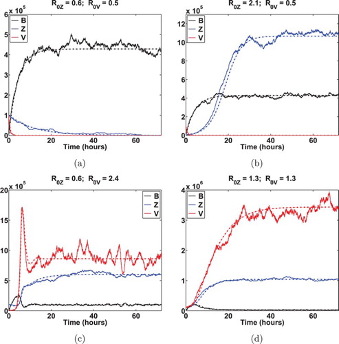
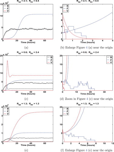
Figure 4. Illustration of disease extinction by displaying a sample path of the stochastic model (19(19) $\begin{array}{rl}B\left(t\right)& =B\left(0\right)+{\mathit{N}}_1\left({\int }_0^t\mathrm{\Lambda }\mathrm{d}u\right)-{\mathit{N}}_2\left({\int }_0^t\alpha \frac{B\left(u\right)}{\kappa +B\left(u\right)}V\right(u\left)\mathrm{d}u\right)-{\mathit{N}}_3\left({\int }_0^t{\delta }_{1}B\right(u\left)\mathrm{d}u\right),\\ Z\left(t\right)& =Z\left(0\right)+{\mathit{N}}_4\left({\int }_0^{t}g\right(Z\left(u\right)\left)\mathrm{d}u\right)+{\mathit{N}}_2\left({\int }_0^t\alpha \frac{B\left(u\right)}{\kappa +B\left(u\right)}V\right(u\left)\mathrm{d}u\right)\\ & +{\mathit{N}}_5\left({\int }_0^t\right({\theta }_1-1\left)\alpha \frac{B\left(u\right)}{\kappa +B\left(u\right)}V\right(u\left)\mathrm{d}u\right)-{\mathit{N}}_6\left({\int }_0^t{\delta }_{2}Z\right(u\left)\mathrm{d}u\right),\\ V\left(t\right)& =V\left(0\right)+{\mathit{N}}_7\left({\int }_0^{t}h\right(V\left(u\right)\left)\mathrm{d}u\right)+{\mathit{N}}_2\left({\int }_0^t\alpha \frac{B\left(u\right)}{\kappa +B\left(u\right)}V\right(u\left)\mathrm{d}u\right)\\ & +{\mathit{N}}_8\left({\int }_0^t\right({\theta }_2-1\left)\alpha \frac{B\left(u\right)}{\kappa +B\left(u\right)}V\right(u\left)\mathrm{d}u\right)-{\mathit{N}}_9\left({\int }_0^t{\delta }_{3}V\right(u\left)\mathrm{d}u\right),\end{array}$(19) ) as compared to the corresponding solution of ordinary differential equation (ODE) (1(1) $\begin{array}{rl}\frac{\mathrm{d}B}{\mathrm{d}t}& =\mathrm{\Lambda }-\alpha \frac{B}{\kappa +B}V-{\delta }_{1}B,\\ \frac{\mathrm{d}Z}{\mathrm{d}t}& =g\left(Z\right)+{\theta }_1\alpha \frac{B}{\kappa +B}V-{\delta }_{2}Z,\\ \frac{\mathrm{d}V}{\mathrm{d}t}& =h\left(V\right)+{\theta }_2\alpha \frac{B}{\kappa +B}V-{\delta }_{3}V,\end{array}$(1) ). Here, the solid and dashed curves represent a sample path of the stochastic model and the associated ODE model, respectively. It shows that the ODE solution approaches the VFE (see the top panel) or EE (see the middle and bottom panels), whereas the corresponding sample path of the stochastic model can go to extinction (see the panel on the right). The parameter values are the same as that of Figure 3. Initial conditions: (a) $(B,Z,V)\left(0\right)=(2\times {10}^4,8,2)$; (b) and (c) $(B,Z,V)\left(0\right)=(2\times {10}^4,5,5)$.

Case 1: $R_{0Z}<1$ and $R_{0V}<1$. This is illustrated in Figure 3(a), and $R_{0Z}=0.6$ and $R_{0V}=0.5$ in the displayed example. It shows that sample paths of our stochastic model are very likely to be close to the associated deterministic solution, and both deterministic and stochastic models indicate the disease extinction. Moreover, in this case, for every set of parameter values within biologically feasible ranges, and for initial conditions that are near the IFE, we have numerically confirmed that the disease extinction probability is very close to one. Here, extinction probability is estimated by computing the proportion of 10,000 sample paths that hit zero. When initial conditions are not close to the IFE, for instance, $(B,Z,V)\left(0\right)=(6\times {10}^3,{10}^5,{10}^5)$, sample paths of stochastic model are still likely to fluctuate around the associated ODE solution. Meanwhile, we see from this example that the virus population decays exponentially and approaches to zero in about 5 h, and human vibrios population decreases linearly and goes to zero after 66 h or so. This sample path indicates that disease extinction within a human host occurs in about 66 h.

Case 2: $R_{0Z}>1$ and $R_{0V}<1$. As one can see from Figure 3(b), the ODE solution converges to the VFE and hence the deterministic model indicates the persistence of environmental and human bacteria. In contrast, the stochastic model shows that bacterium populations can either persist (displayed in Figure 3(b)), or go extinct (displayed in Figure 4(a, b)). Case 3: $R_{0Z}<1$ and $R_{0V}>1$ and Case 4: $R_{0Z}>1$ and $R_{0V}>1$. In both scenarios, deterministic dynamics indicate the occurrence of an outbreak, which is illustrated in Figures 3(c, d), and 4(c, e). However, the stochastic model, more realistically, shows that disease can go extinct within the human host (illustrated in Figure 4(c–f)). Indeed, Theorem 3.1 demonstrates that this extinction has a positive probability.

Let $P_0^{\mathrm{ext}}$ denote the probability of disease extinction computed from the branching process approximation. Let $P_0^{\mathrm{MC}}$ be an estimate obtained from the fraction of sample paths (out of 10,000) in which both $Z\left(t\right)$ and $V\left(t\right)$ hit zero before reaching VFE/EE levels. Applying Theorem 3.1, we calculate explicit estimate $P_0^{\mathrm{ext}}$ and then compare to the corresponding estimate $P_0^{\mathrm{MC}}$ obtained from Monte Carlo simulation. A summary of results for various initial conditions in Cases 2–4 is displayed in Table 2. It shows that $P_0^{\mathrm{ext}}$ is a good estimate of the disease extinction probability. For instance, in the first example, $R_{0Z}=0.64<1$, $R_{0V}=2.36>1$, and $V\left(0\right)=v_0=1$. By Theorem 3.1, $P_0^{\mathrm{ext}}=(1/R_{0V}{)}^{v_0}=0.4242$. Comparing this with $P_0^{\mathrm{MC}}=0.4236$, we see that the theoretical approximation $P_0^{\mathrm{ext}}$ is very close to its numerical approximation $P_0^{\mathrm{MC}}$ based on sample paths.

Table 2. Disease extinction probability estimated by using the branching process approximation, $P_0^{\mathrm{ext}}$, vs. the associated estimate based on Monte Carlo simulations of 10,000 sample paths of (19(19) $\begin{array}{rl}B\left(t\right)& =B\left(0\right)+{\mathit{N}}_1\left({\int }_0^t\mathrm{\Lambda }\mathrm{d}u\right)-{\mathit{N}}_2\left({\int }_0^t\alpha \frac{B\left(u\right)}{\kappa +B\left(u\right)}V\right(u\left)\mathrm{d}u\right)-{\mathit{N}}_3\left({\int }_0^t{\delta }_{1}B\right(u\left)\mathrm{d}u\right),\\ Z\left(t\right)& =Z\left(0\right)+{\mathit{N}}_4\left({\int }_0^{t}g\right(Z\left(u\right)\left)\mathrm{d}u\right)+{\mathit{N}}_2\left({\int }_0^t\alpha \frac{B\left(u\right)}{\kappa +B\left(u\right)}V\right(u\left)\mathrm{d}u\right)\\ & +{\mathit{N}}_5\left({\int }_0^t\right({\theta }_1-1\left)\alpha \frac{B\left(u\right)}{\kappa +B\left(u\right)}V\right(u\left)\mathrm{d}u\right)-{\mathit{N}}_6\left({\int }_0^t{\delta }_{2}Z\right(u\left)\mathrm{d}u\right),\\ V\left(t\right)& =V\left(0\right)+{\mathit{N}}_7\left({\int }_0^{t}h\right(V\left(u\right)\left)\mathrm{d}u\right)+{\mathit{N}}_2\left({\int }_0^t\alpha \frac{B\left(u\right)}{\kappa +B\left(u\right)}V\right(u\left)\mathrm{d}u\right)\\ & +{\mathit{N}}_8\left({\int }_0^t\right({\theta }_2-1\left)\alpha \frac{B\left(u\right)}{\kappa +B\left(u\right)}V\right(u\left)\mathrm{d}u\right)-{\mathit{N}}_9\left({\int }_0^t{\delta }_{3}V\right(u\left)\mathrm{d}u\right),\end{array}$(19) ), $P_0^{\mathrm{MC}}$.

Scenario	$z_0$	$v_0$	$P_0^{\mathrm{ext}}$	$P_0^{\mathrm{MC}}$
$R_{0Z}=0.64,R_{0V}=2.36$	1	1	0.4242	0.4236
	1	2	0.1800	0.1782
	2	1	0.4242	0.4291
$R_{0Z}=2.14,R_{0V}=0.51$	1	1	0.4667	0.4653
	1	2	0.4667	0.4601
	2	1	0.2178	0.2209
$R_{0Z}=1.29,R_{0V}=1.29$	1	1	0.6508	0.6523
	1	2	0.5446	0.5429
	2	1	0.5062	0.5107

Note: The parameter values are the same as that of Figure 3.

5. Discussion

We have proposed a new modelling framework for the within-host dynamics of cholera, using both deterministic and stochastic formulations. Our focus is the interaction of environmental vibrios (with low infectivity), human vibrios (with high infectivity), and the virus (which causes the transformation from environmental vibrios to human vibrios) within a human host. Such an interaction is critical in shaping the evolution of the pathogen within human body and directly contributes to the epidemiology of cholera at the population level, since the human vibrios shed out of human body will remain highly infectious for a certain period of time and can be transmitted among human hosts.

For our deterministic model, we have calculated the basic reproduction number, $R_0$, which consists of two components: one represents the intrinsic growth of the human vibrios and the other accounts for the viral–bacterial interaction. We have established the basic reproduction number as a sharp threshold for disease dynamics: when $R_0<1$, the highly infectious vibrios will not grow within the human host and the environmental vibrios ingested into human body will not cause cholera infection; when $R_0>1$, the human vibrios will grow and persist, leading to human cholera. We have found that while there is only one equilibrium (the IFE) when $R_0<1$, there can be two or three equilibria when $R_0>1$ that include the IFE and one or both the VFE and EE. The existence and stabilities of these equilibria characterize the essential dynamics of the model, and we have conducted both local and global stability analysis for each equilibrium.

For our stochastic model, based on the MJP, we have focused our attention on the probability of disease extinction within a human host which provides an estimate of the disease risk under some realistic conditions (e.g. small amount of initial infection, small number of bacteria or virus). We have derived an explicit expression for the probability of disease extinction, and verified the result through careful numerical simulation involving a large number of sample paths. We have also carefully compared the numerical simulation results from the deterministic model and the stochastic model.

As can be expected, analysis of our deterministic model can provide more detailed information regarding the disease dynamics, and a single quantity, $R_0$, can be used as a disease threshold. Nevertheless, the stochastic model can provide an important estimate of the disease risk under situations where the assumption of homogeneous mixing of bacteria or virus does not hold and where the randomness should be taken into account. Hence, both models are useful in studying cholera and, together, they could give us a more complete picture toward understanding the within-host dynamics of cholera.

Our future plan is to couple this within-host modelling framework with an epidemiological cholera model, linking the within-host and between-host dynamics of cholera in a more biologically meaningful way. Using such an integrated model, we will carefully investigate the bacterial–viral interaction within human host, the human–human and human–environment interaction at the population level, and their impacts to each other toward shaping the complex, multi-scale dynamics of cholera. We will again explore both deterministic and stochastic formulations, and compare and integrate the findings from each approach.

Acknowledgements

The authors would like to thank the anonymous reviewers and the editor for their suggestions that have improved this paper.

Disclosure statement

No potential conflict of interest was reported by the authors.

Additional information

Funding

This work was partially supported by a grant from the http://dx.doi.org/10.13039/100000893 Simons Foundation (#317047 to Xueying Wang). Jin Wang was partially supported by the http://dx.doi.org/10.13039/100000001 National Science Foundation [grant numbers 1412826, 1520672, and 1557739].

References

- L.J.S. Allen and G.E. Lahodny Jr., Extinction thresholds in deterministic and stochastic epidemic models, J. Biol. Dyn. 6 (2012), pp. 590–611. doi: 10.1080/17513758.2012.665502
- L.J.S. Allen and P. van den Driessche, Relations between deterministic and stochastic thresholds for disease extinction in continuous- and discrete-time infectious disease models, Math. Biosci. 243 (2013), pp. 99–108. doi: 10.1016/j.mbs.2013.02.006
- R.M. Anderson and R.M. May, Infectious Diseases of Humans: Dynamics and Control, Oxford University Press, Oxford, UK, 1991.
- K.B. Athreya and P.E. Ney, Branching Processes, Springer, New York, 1972.
- V. Capasso and S.L. Paveri-Fontana, A mathematical model for the 1973 cholera epidemic in the European Mediterranean region, Rev. Epidemiol. Sante 27(2) (1979), pp. 121–132.
- A. Carpenter, Behavior in the time of cholera: Evidence from the 2008–2009 cholera outbreak in Zimbabwe, in Social Computing, Behavioral-Cultural Modeling and Prediction, Vol. 8393, W.G. Kennedy, N. Agarwal, and S.J. Yang, eds., Lecture Notes in Computer Science, Springer, Berlin, pp. 237–244.
- R.R. Colwell, A global and historical perspective of the genus Vibrio, in The Biology of Vibrios, F.L. Thompson, B. Austin, and J. Swings, eds., ASM Press, Washington, DC, 2006.
- K.S. Dorman, J.S. Sinsheimer, and K. Lange, In the garden of branching processes, SIAM Rev. 46 (2004), pp. 202–229. doi: 10.1137/S0036144502417843
- S.M. Faruque and G.B. Nair, Vibrio cholerae: Genomics and Molecular Biology, Caister Academic Press, Norfolk, UK, 2008.
- T.E. Harris, The Theory of Branching Processes, Springer, Berlin, 1963.
- D.M. Hartley, J.G. Morris, and D.L. Smith, Hyperinfectivity: A critical element in the ability of V. cholerae to cause epidemics?, PLoS Med. 3 (2006), pp. 0063–0069. doi: 10.1371/journal.pmed.0030063
- P. Jagers, Branching Processes with Biological Applications, John, London, 1975.
- S.T. Karlin and H.M. Taylor, A First Course in Stochastic Processes, 2nd ed., Academic Press, San Diego, CA, 1975.
- J.P. LaSalle, The Stability of Dynamical Systems, Regional Conference Series in Applied Mathematics, SIAM, Philadelphia, PA, 1976.
- Z. Mukandavire, S. Liao, J. Wang, H. Gaff, D.L. Smith, and J.G. Morris, Estimating the reproductive numbers for the 2008–2009 cholera outbreaks in Zimbabwe, Proc. Nat. Acad. Sci. USA 108 (2011), pp. 8767–8772. doi: 10.1073/pnas.1019712108
- R.L.M. Neilan, E. Schaefer, H. Gaff, K.R. Fister, and S. Lenhart, Modeling optimal intervention strategies for cholera, Bull. Math. Biol. 72 (2010), pp. 2004–2018. doi: 10.1007/s11538-010-9521-8
- E.J. Nelson, J.B. Harris, J.G. Morris, S.B. Calderwood, and A. Camilli, Cholera transmission: The host, pathogen and bacteriophage dynamics, Nat. Rev. Microbiol. 7 (2009), pp. 693–702. doi: 10.1038/nrmicro2204
- D. Posny and J. Wang, Modelling cholera in periodic environments, J. Biol. Dyn. 8(1) (2014), pp. 1–19. doi: 10.1080/17513758.2014.896482
- D. Posny, J. Wang, Z. Mukandavire, and C. Modnak, Analyzing transmission dynamics of cholera with public health interventions, Math. Biosci. 264 (2015), pp. 38–53. doi: 10.1016/j.mbs.2015.03.006
- Z. Shuai and P. van den Driessche, Global dynamics of cholera models with differential infectivity, Math. Biosci. 234(2) (2011), pp. 118–126. doi: 10.1016/j.mbs.2011.09.003
- Z. Shuai and P. van den Driessche, Global stability of infectious disease models using Lyapunov functions, SIAM J. Appl. Math. 73(4) (2013), pp. 1513–1532. doi: 10.1137/120876642
- J.P. Tian and J. Wang, Global stability for cholera epidemic models, Math. Biosci. 232(1) (2011), pp. 31–41. doi: 10.1016/j.mbs.2011.04.001
- J.H. Tien and D.J.D. Earn, Multiple transmission pathways and disease dynamics in a waterborne pathogen model, B. Math. Biol. 72(6) (2010), pp. 1506–1533. doi: 10.1007/s11538-010-9507-6
- P. van den Driessche and J. Watmough, Reproduction numbers and sub-threshold endemic equilibria for compartmental models of disease transmission, Math. Biosci. 180 (2002), pp. 29–48. doi: 10.1016/S0025-5564(02)00108-6
- O.A. van Herwaarden and J. Grasman, Stochastic epidemics: Major outbreaks and the duration of the endemic period, J. Math. Biol. 33 (1995), pp. 581–601. doi: 10.1007/BF00298644
- J. Wang and S. Liao, A generalized cholera model and epidemic-endemic analysis, J. Biol. Dyn. 6(2) (2012), pp. 568–589. doi: 10.1080/17513758.2012.658089
- X. Wang and J. Wang, Analysis of cholera epidemics with bacterial growth and spatial movement, J. Biol. Dyn. 9(1) (2015), pp. 233–261. doi: 10.1080/17513758.2014.974696
- X. Wang and J. Wang, Disease dynamics in a coupled cholera model linking within-host and between-host interactions, J. Biol. Dyn., doi:10.1080/17513758.2016.1231850
- X. Wang, D. Gao, and J. Wang, Influence of human behavior on cholera dynamics, Math. Biosci. 267 (2015), pp. 41–52. doi: 10.1016/j.mbs.2015.06.009
- S. Wiggins, Introduction to Applied Nonlinear Dynamical Systems and Chaos, 2nd ed., Springer, New York, 2003.
- K. Yamazaki and X. Wang, Global well-posedness and asymptotic behavior of solutions to a reaction-convection-diffusion cholera epidemic model, Discrete Contin. Dyn. Syst. Ser. B 21 (2016), pp. 1297–1316. doi: 10.3934/dcdsb.2016.21.1297
- K. Yamazaki and X. Wang, Global stability and uniform persistence of the reaction-convection-diffusion cholera epidemic model, Math. Biosci. Eng. 14(2) (2017), pp. 559–579.