The travelling wave of Gray-Scott systems – existence, multiplicity and stability

ABSTRACT

This article studies existence and stability of travelling wave of unstirred Gray-Scott system in biological pattern formation which models an isothermal chemical reaction $A+2B\to 3B$ involving two chemical species, a reactant A and an auto-catalyst B, and a linear decay $B\to C$, where C is an inert product. Our result shows a new and very distinctive feature of Gray-Scott type of models in generating rich and structurally different travelling pulses than related models in the literature. In particular, the existence of multiple travelling waves which have distinctive number of local maxima is proved. Furthermore, the stability of travelling wave of the reaction–diffusion system of isothermal diffusion system $A+2B\to 3B$, is also studied.

KEYWORDS:

• Gray-Scott model
• travelling wave
• multi-peak waves
• stability
• spreading of local disturbance

AMS SUBJECT CLASSIFICATIONS:

• 34C20
• 34C25
• 92E20

1. Introduction

In this paper, we consider $\left(\mathrm{I}\right)\{\begin{array}{l}\frac{\mathrm{\partial }u}{\mathrm{\partial }t}=\frac{{\mathrm{\partial }}^{2}u}{\mathrm{\partial }{x}^2}-u{v}^m,\\ \frac{\mathrm{\partial }v}{\mathrm{\partial }t}=D\frac{{\mathrm{\partial }}^{2}v}{\mathrm{\partial }{x}^2}+u{v}^m-k{v}^l.\end{array}$

It models chemical reaction of the form $A+mB\to (m+1)B\text{with rate }u{v}^m\text{ and }B\to C$ with C being an inert chemical species. Here, D, a positive constant, is the ratio of diffusion coefficients of chemical species B to that of A, $m\ge 1$ is a positive constant not necessarily an integer, and $k{v}^l$ describes the rate of $B\to C$, with k and $l\ge 1$ both positive constants. We assume throughout that $1\le l<m$.

Many models in mathematical biology take the form of system (I), see [10, 14, 17]. In particular, m=2 and l=1 is the famous Gray-Scott model in biological pattern formation, one of the popular models proposed for replicating experiment results in early 1990s, see [13, 14]. The most exciting feature of the diffusive Gray-Scott system with feeding is self-replicating travelling pulse (travelling wave). It has been extensively studied, see [7, 8, 11] by formal analysis and numerical computation, but the phenomenon and underlying mechanism is not completely understood. In particular, rigorous analysis of Gray-Scott is badly needed.

Our main concern is the existence and stability of travelling wave to (I) and a related system (II) below. A travelling wave solution for (I) links one equilibrium point to another. Since any equilibrium point of (I) is of the form $(a,0)$, $a\in \mathbb{R}$, the travelling wave problem takes the from (1) $\begin{array}{rl}{u}^{″}+c{u}^{\prime }& =u{v}^m,u^{\prime }>0\text{in}\mathbb{R},\\ D{v}^{″}+c{v}^{\prime }& =k{v}^l-u{v}^m,v>0\text{in}\mathbb{R},\\ u(-\mathrm{\infty })& =u_0>0,v(-\mathrm{\infty })=0,v\left(\mathrm{\infty }\right)=0,u\left(\mathrm{\infty }\right)<\mathrm{\infty }.\end{array}$(1)

It is easy to show that the travelling wave solution to (I) exists only when $m\ge l$. This is because with $u_0>0$ we need $k{v}^m\ge u{v}^l$ for all x close to $-\mathrm{\infty }$ to make v positive for all x close to $-\mathrm{\infty }$. In case of l>m, it is proved in [9] that (I) has a travelling wave solution when $u_0=0$. The dynamics of that model is very different from our case.

The travelling wave problem (1(1) $\begin{array}{rl}{u}^{″}+c{u}^{\prime }& =u{v}^m,u^{\prime }>0\text{in}\mathbb{R},\\ D{v}^{″}+c{v}^{\prime }& =k{v}^l-u{v}^m,v>0\text{in}\mathbb{R},\\ u(-\mathrm{\infty })& =u_0>0,v(-\mathrm{\infty })=0,v\left(\mathrm{\infty }\right)=0,u\left(\mathrm{\infty }\right)<\mathrm{\infty }.\end{array}$(1) ) with m>l, is very different from any of the main types of scalar equation as well as other related models such as the case of l=m, see [6] for more details or the system (II) below of isothermal diffusion system without decay. In particular, for l=m or system (II), the travelling wave problem is of the mono-stable case of scalar equation, but our case is not.

For simplicity, we shall only treat the case of l=1, m>1 in details in this work. For the case of m>l>1, we refer the reader to [20]. By a simple scaling, we can scale out k, and hence, we assume k=1 here and in Section 2.

The following result is proved in [6] which shows a complete different and unique feature of Gray-Scott type of models.

Theorem A

Let $D>0,$ $m>1,$ $k=l=1,$ and $u_0>0$ be given constants. There exists a positive constant c such that (1(1) $\begin{array}{rl}{u}^{″}+c{u}^{\prime }& =u{v}^m,u^{\prime }>0\text{in}\mathbb{R},\\ D{v}^{″}+c{v}^{\prime }& =k{v}^l-u{v}^m,v>0\text{in}\mathbb{R},\\ u(-\mathrm{\infty })& =u_0>0,v(-\mathrm{\infty })=0,v\left(\mathrm{\infty }\right)=0,u\left(\mathrm{\infty }\right)<\mathrm{\infty }.\end{array}$(1) ) admits a solution. In addition, the set of speeds for existence lies in a bounded interval for a given value of $u_0>0$. Furthermore, the speed c must satisfy $c^2<2D[max(1,D){\left(\frac{m+1}{2u_0}\right)}^{m/(m-1)}\frac{m+1}{m-1}+m-1].$

That is, our travelling wave problem is not mono-stable type, nor the bistable type as our main result below shows.

Perhaps, the most exciting and surprising result is the one which shows when $u_0\gg 1$, there exists a large number of travelling wave solutions, each with fixed number of local maxima for $w=u{v}^{m-1}$ and with different speed. For this, we re-cast (1(1) $\begin{array}{rl}{u}^{″}+c{u}^{\prime }& =u{v}^m,u^{\prime }>0\text{in}\mathbb{R},\\ D{v}^{″}+c{v}^{\prime }& =k{v}^l-u{v}^m,v>0\text{in}\mathbb{R},\\ u(-\mathrm{\infty })& =u_0>0,v(-\mathrm{\infty })=0,v\left(\mathrm{\infty }\right)=0,u\left(\mathrm{\infty }\right)<\mathrm{\infty }.\end{array}$(1) ), after simple scaling, as (2) $\begin{array}{rl}d{u}^{″}+c{u}^{\prime }& =u{v}^m,u^{\prime }>0\text{in}\mathbb{R},\\ v^{″}+c{v}^{\prime }& =v-u{v}^m,v>0\text{in}\mathbb{R},\\ u(-\mathrm{\infty })& =h,v(-\mathrm{\infty })=0,v\left(\mathrm{\infty }\right)=0,u\left(\mathrm{\infty }\right)<\mathrm{\infty },\end{array}$(2) where $d=D^{-1}$. We make the following change of scale and variables: $\epsilon =h^{-m/(m-1)},u=[1+\epsilon u^{\ast }]h,v=h^{-1/(n-1)}{v}^{\ast },c=c^{\ast }\epsilon .$

Then (1(1) $\begin{array}{rl}{u}^{″}+c{u}^{\prime }& =u{v}^m,u^{\prime }>0\text{in}\mathbb{R},\\ D{v}^{″}+c{v}^{\prime }& =k{v}^l-u{v}^m,v>0\text{in}\mathbb{R},\\ u(-\mathrm{\infty })& =u_0>0,v(-\mathrm{\infty })=0,v\left(\mathrm{\infty }\right)=0,u\left(\mathrm{\infty }\right)<\mathrm{\infty }.\end{array}$(1) ) is equivalent to finding $(u^{\ast },v^{\ast },c^{\ast })\in C^2\left(\mathbb{R}\right)\times C^2\left(\mathbb{R}\right)\times (0,\mathrm{\infty })$ which satisfy, after dropping ‘${}^{\ast }$’, (3) $\begin{array}{rl}d{u}^{″}+c\epsilon u^{\prime }& =[1+\epsilon u]v^m,u^{\prime }>0\text{in}\mathbb{R},\\ v^{″}+c\epsilon v^{\prime }& =v-[1+\epsilon u]v^m,v>0\text{in}\mathbb{R},\\ u(-\mathrm{\infty })& =0,v(-\mathrm{\infty })=0,v\left(\mathrm{\infty }\right)=0,u\left(\mathrm{\infty }\right)<\mathrm{\infty }.\end{array}$(3)

Define (4) $\begin{array}{rl}G\left(s\right)& =s^2-\frac{2s_{+}^{m+1}}{m+1},\alpha =\frac{1}{m-1},M={\left(\frac{m+1}{2}\right)}^{\alpha },\\ \sigma & =4{\int }_0^M\sqrt{G\left(s\right)}\mathrm{d}s,\gamma =\frac{2\alpha }{D}{\int }_0^M\frac{s^m\mathrm{d}s}{\sqrt{G\left(s\right)}},\end{array}$(4) $s_{+}=max\{s,0\}$. Our main result on travelling wave of (I) is the following theorem.

Theorem 1.1

Let m>1 and D>0 be given constants.

1. There exist positive constants $M_1,$ $M_2,$ and $M_3$ that depend only on m and D such that for each $\epsilon >0,$ Equation (3(3) $\begin{array}{rl}d{u}^{″}+c\epsilon u^{\prime }& =[1+\epsilon u]v^m,u^{\prime }>0\text{in}\mathbb{R},\\ v^{″}+c\epsilon v^{\prime }& =v-[1+\epsilon u]v^m,v>0\text{in}\mathbb{R},\\ u(-\mathrm{\infty })& =0,v(-\mathrm{\infty })=0,v\left(\mathrm{\infty }\right)=0,u\left(\mathrm{\infty }\right)<\mathrm{\infty }.\end{array}$(3) ) admits no solution if $c⩾max\{\sqrt{M_1/\epsilon },M_2\}$ or if $c⩽\gamma -M_3\epsilon$.

2. For each sufficiently small positive $\epsilon$ and each integer L satisfying $1⩽L⩽{\epsilon }^{-1/4},$ there exists a constant $c_L=L\gamma [1+O(\epsilon +[L-1{]}^2\epsilon |\ln \epsilon |)]$ such that when $c=c_L,$ the system (3(3) $\begin{array}{rl}d{u}^{″}+c\epsilon u^{\prime }& =[1+\epsilon u]v^m,u^{\prime }>0\text{in}\mathbb{R},\\ v^{″}+c\epsilon v^{\prime }& =v-[1+\epsilon u]v^m,v>0\text{in}\mathbb{R},\\ u(-\mathrm{\infty })& =0,v(-\mathrm{\infty })=0,v\left(\mathrm{\infty }\right)=0,u\left(\mathrm{\infty }\right)<\mathrm{\infty }.\end{array}$(3) ) admits a solution, unique up to a translation. The solution is an L-hump solution in the sense that $w:=[1+\epsilon u]v^{m-1}$ admits exactly L local maxima and L−1 interior local minima. In addition, if denote the interior points of local minima of w by $\{a_i{\}}_{i=2}^{L-1}$ and points of local maxima by $\{b_i{\}}_{i=1}^L$ with $-\mathrm{\infty }=a_1<b_1<a_2<b_2<\cdots <b_L<a_{L+1}=\mathrm{\infty },$ then $\begin{array}{rl}w\left(b_i\right)& =M+O\left(i\right[L+1-i\left]\epsilon \right),\\ G\left(w\right(a_{i+1}\left)\right)& =i(L-i)\sigma \gamma \epsilon +O\left(i^2{L}^2{\epsilon }^2|\ln \epsilon |\right)\mathrm{\forall }i=1,\dots ,L.\end{array}$

   Furthermore, $\parallel w^{\prime 2}-G\left(w\right){\parallel }_{L^{\mathrm{\infty }}\left(\mathbb{R}\right)}=O\left(L^2\epsilon \right)$ and $\underset{\epsilon \searrow 0}{lim}w(b_i+z)=\underset{\epsilon \searrow 0}{lim}v(b_i+z)=W\left(z\right)$ uniformly in $i=1,\dots ,L$ and locally uniformly in $z\in \mathbb{R},$ where W is the unique solution of (5) $W^{″}=W-W^m\mathrm{in}\mathbb{R},W\left(0\right)=M,W^{\prime }\left(0\right)=0.$(5)

Remark 1.1

It is clear that since u is strictly increasing, the L-hump solution must have at least L local maxima for v, thus a travelling wave solution with a large number of oscillations. As a matter of fact, it should be clear from our proof that as $\epsilon \to 0$, v has exactly L-hump.

In addition, the solution W of Equation (5(5) $W^{″}=W-W^m\mathrm{in}\mathbb{R},W\left(0\right)=M,W^{\prime }\left(0\right)=0.$(5) ) is a closed orbit, our result can be explained as that v is a small perturbation of W when $\epsilon$ is small. But, since our system does not admit any close orbit, v has to decay to zero exponentially with a rate uniquely determined by the corresponding travelling wave speed.

Another reaction–diffusion system, we would like to pursue models the following simple isothermal chemical reaction: $A+mB\to (m+1)B\text{with rate}ka{b}^m\text{and }m=1,2$ between two chemical species A and B, where k>0 is the rate constant. It appears in many chemical wave models of excitable media ranging from the idealized Brusselator to real-world clock reactions such as Belousov–Zhabotinsky reaction, the Briggs–Rauscher reaction, the Bray–Liebhafsky reaction and the iodine clock reaction. In those setting, its importance was recognized pretty early, [10, 18].

In this work, we study the travelling wave problem of autocatalytic chemical reaction $A+mB\to (m+1)B$, which, after simple non-dimensionalization, results in the reaction–diffusion system, $\left(\mathrm{II}\right)\{\begin{array}{l}\frac{\mathrm{\partial }u}{\mathrm{\partial }t}=\frac{{\mathrm{\partial }}^{2}u}{\mathrm{\partial }{x}^2}-u{v}^m,\\ \frac{\mathrm{\partial }v}{\mathrm{\partial }t}=D\frac{{\mathrm{\partial }}^{2}v}{\mathrm{\partial }{x}^2}+u{v}^m.\end{array}$

For a travelling wave solution to (II), $u(x,t)=u\left(z\right),v(x,t)=v\left(z\right)$, where z=x−ct, the governing ODE system is (6) $u^{″}+c{u}^{\prime }-u{v}^m=0,D{v}^{″}+c{v}^{\prime }+u{v}^m=0,$(6) where c>0 is a constant. Assuming $\underset{z\to -\mathrm{\infty }}{lim}(u,v)=(0,a),a>0,$

It is easy to prove that for a travelling wave solution, $\underset{z\to \mathrm{\infty }}{lim}(u,v)=(a,0)$. By a simple scaling, we only need to consider a=1, the travelling wave problem of (II) is the following: (7) $\begin{array}{rl}{u}^{″}+c{u}^{\prime }& =u{v}^m,u^{\prime }⩾0\mathrm{\forall }z\in \mathbb{R},\\ D{v}^{″}+c{v}^{\prime }& =-u{v}^m,v⩾0\mathrm{\forall }z\in \mathbb{R},\\ \underset{z\to \mathrm{\infty }}{lim}(u,v)& =(1,0),\underset{z\to -\mathrm{\infty }}{lim}(u,v)=(0,1).\end{array}$(7)

It turns out the travelling wave problem of (II) is of the mono-stable type for scalar equation with a minimum positive speed. The main effort is then to prove sharp bound on minimum speed, because the minimum speed travelling wave is the most stable one. The following two results are proved in [4, 5].

Theorem B

Suppose D<1 and m>1. There exists no travelling wave of Equation (7(7) $\begin{array}{rl}{u}^{″}+c{u}^{\prime }& =u{v}^m,u^{\prime }⩾0\mathrm{\forall }z\in \mathbb{R},\\ D{v}^{″}+c{v}^{\prime }& =-u{v}^m,v⩾0\mathrm{\forall }z\in \mathbb{R},\\ \underset{z\to \mathrm{\infty }}{lim}(u,v)& =(1,0),\underset{z\to -\mathrm{\infty }}{lim}(u,v)=(0,1).\end{array}$(7) ) if $c⩽\sqrt{\frac{D}{K\left(m\right)}}\frac{1}{\sqrt{1-(1-\frac{1}{D})\frac{\sqrt{4K\left(m\right)+1}-1}{\sqrt{4K\left(m\right)+1}+1}}}.$ where $K\left(m\right)$ is a constant which depends on m only and is an increasing function of m. In particular, $K\left(1\right)=1/4,$ $K\left(2\right)=2$. For existence, we have the following results.

1. If $m⩾2,$ a unique $($up to translation$)$ travelling wave solution exists for (7(7) $\begin{array}{rl}{u}^{″}+c{u}^{\prime }& =u{v}^m,u^{\prime }⩾0\mathrm{\forall }z\in \mathbb{R},\\ D{v}^{″}+c{v}^{\prime }& =-u{v}^m,v⩾0\mathrm{\forall }z\in \mathbb{R},\\ \underset{z\to \mathrm{\infty }}{lim}(u,v)& =(1,0),\underset{z\to -\mathrm{\infty }}{lim}(u,v)=(0,1).\end{array}$(7) ) for each $c\ge 4D/\sqrt{1+4D}.$

2. If $1<m<2,$ a unique $($up to translation$)$ travelling wave solution exists for Equation (7(7) $\begin{array}{rl}{u}^{″}+c{u}^{\prime }& =u{v}^m,u^{\prime }⩾0\mathrm{\forall }z\in \mathbb{R},\\ D{v}^{″}+c{v}^{\prime }& =-u{v}^m,v⩾0\mathrm{\forall }z\in \mathbb{R},\\ \underset{z\to \mathrm{\infty }}{lim}(u,v)& =(1,0),\underset{z\to -\mathrm{\infty }}{lim}(u,v)=(0,1).\end{array}$(7) ) for each $c\ge \frac{2D}{(-D^2+{\nu }^2{)}^{1/2}},\mathrm{where}\nu =\frac{m-1+\sqrt{(m-1{)}^2+8(3-m)D+16D^2}}{4}.$

Theorem C

Suppose $D⩾1$ and $m⩾1$. There exists a positive constant $c_{min}$ such that Equation (7(7) $\begin{array}{rl}{u}^{″}+c{u}^{\prime }& =u{v}^m,u^{\prime }⩾0\mathrm{\forall }z\in \mathbb{R},\\ D{v}^{″}+c{v}^{\prime }& =-u{v}^m,v⩾0\mathrm{\forall }z\in \mathbb{R},\\ \underset{z\to \mathrm{\infty }}{lim}(u,v)& =(1,0),\underset{z\to -\mathrm{\infty }}{lim}(u,v)=(0,1).\end{array}$(7) ) has a travelling wave if and only if $c⩾c_{min}$. In addition, $c_{min}$ is bounded by $\sqrt{\frac{D}{K\left(m\right)}}⩽c_{min}⩽\sqrt{\frac{D}{K\left(m\right)}}\frac{1}{\sqrt{1-(1-\frac{1}{D})\frac{\sqrt{4K\left(m\right)+1}-1}{\sqrt{4K\left(m\right)+1}+1}}},$ where $K\left(m\right)$ is the same constant as in above theorem.

It is clear from the above two results that $c_{min}$ is of order $O\left(D\right)$ if $0<D\ll 1$, but $O\left(\sqrt{D}\right)$ if $D\gg 1$.

Our main focus on (II) is to study stability of travelling waves using combination of rigorous analysis and numerical computation. Our results on (II) are stated and proved in Section 3.

For related works on existence, stability and global dynamics of (I) or (II), we refer the reader to [3, 12, 16, 19, 21].

The organization of the paper is as follows. In Section 2, we study the system (3(3) $\begin{array}{rl}d{u}^{″}+c\epsilon u^{\prime }& =[1+\epsilon u]v^m,u^{\prime }>0\text{in}\mathbb{R},\\ v^{″}+c\epsilon v^{\prime }& =v-[1+\epsilon u]v^m,v>0\text{in}\mathbb{R},\\ u(-\mathrm{\infty })& =0,v(-\mathrm{\infty })=0,v\left(\mathrm{\infty }\right)=0,u\left(\mathrm{\infty }\right)<\mathrm{\infty }.\end{array}$(3) ) and prove the existence of multiple travelling waves to system (I), and in Section 3 we analyse the stability of travelling waves of system (II).

2. Existence of multiple travelling waves

In this section we study (3(3) $\begin{array}{rl}d{u}^{″}+c\epsilon u^{\prime }& =[1+\epsilon u]v^m,u^{\prime }>0\text{in}\mathbb{R},\\ v^{″}+c\epsilon v^{\prime }& =v-[1+\epsilon u]v^m,v>0\text{in}\mathbb{R},\\ u(-\mathrm{\infty })& =0,v(-\mathrm{\infty })=0,v\left(\mathrm{\infty }\right)=0,u\left(\mathrm{\infty }\right)<\mathrm{\infty }.\end{array}$(3) ) and prove Theorems 1.1. Due to limited space, we present only key steps of the proof and a more detailed presentation will appear later in [15].

2.1. Preliminary

For each constant $c⩾0$, we consider the initial value problem, for $(u,v)=\left(u\right(x),v(x\left)\right)$, (8) $\begin{array}{rl}d{u}^{″}+c\epsilon u^{\prime }& =[1+\epsilon u]v_{+}^m\text{in}\mathbb{R},\\ v^{″}+c\epsilon v^{\prime }& =v-[1+\epsilon u]v_{+}^m\text{in}\mathbb{R},\\ [v,v^{\prime },u,u^{\prime }]& =[1,\lambda ,0,0]{\mathrm{e}}^{\lambda x}+O\left(1\right){\mathrm{e}}^{m\lambda x}\text{as}x\to -\mathrm{\infty },\end{array}$(8) where λ is the positive root of ${\lambda }^2+c\epsilon \lambda =1$ and $v_{+}:=max\{v,0\}$.

Lemma 2.1

For each $c⩾0,$ problem (8(8) $\begin{array}{rl}d{u}^{″}+c\epsilon u^{\prime }& =[1+\epsilon u]v_{+}^m\text{in}\mathbb{R},\\ v^{″}+c\epsilon v^{\prime }& =v-[1+\epsilon u]v_{+}^m\text{in}\mathbb{R},\\ [v,v^{\prime },u,u^{\prime }]& =[1,\lambda ,0,0]{\mathrm{e}}^{\lambda x}+O\left(1\right){\mathrm{e}}^{m\lambda x}\text{as}x\to -\mathrm{\infty },\end{array}$(8) ), with $\lambda =\sqrt{1+{\epsilon }^2{c}^2/4}-c\epsilon /2,$ admits a unique solution and the solution satisfies $u^{\prime }>0$ in $\mathbb{R}$. In addition, if $(u,v)$ is a solution of Equation (3(3) $\begin{array}{rl}d{u}^{″}+c\epsilon u^{\prime }& =[1+\epsilon u]v^m,u^{\prime }>0\text{in}\mathbb{R},\\ v^{″}+c\epsilon v^{\prime }& =v-[1+\epsilon u]v^m,v>0\text{in}\mathbb{R},\\ u(-\mathrm{\infty })& =0,v(-\mathrm{\infty })=0,v\left(\mathrm{\infty }\right)=0,u\left(\mathrm{\infty }\right)<\mathrm{\infty }.\end{array}$(3) ), then up to a translation, it is the unique solution of Equation (8(8) $\begin{array}{rl}d{u}^{″}+c\epsilon u^{\prime }& =[1+\epsilon u]v_{+}^m\text{in}\mathbb{R},\\ v^{″}+c\epsilon v^{\prime }& =v-[1+\epsilon u]v_{+}^m\text{in}\mathbb{R},\\ [v,v^{\prime },u,u^{\prime }]& =[1,\lambda ,0,0]{\mathrm{e}}^{\lambda x}+O\left(1\right){\mathrm{e}}^{m\lambda x}\text{as}x\to -\mathrm{\infty },\end{array}$(8) ).

The proof is standard and we omit the details. We refer the interested reader to [6].

In the sequel, $(u,v)$ refers to the solution of Equation (8(8) $\begin{array}{rl}d{u}^{″}+c\epsilon u^{\prime }& =[1+\epsilon u]v_{+}^m\text{in}\mathbb{R},\\ v^{″}+c\epsilon v^{\prime }& =v-[1+\epsilon u]v_{+}^m\text{in}\mathbb{R},\\ [v,v^{\prime },u,u^{\prime }]& =[1,\lambda ,0,0]{\mathrm{e}}^{\lambda x}+O\left(1\right){\mathrm{e}}^{m\lambda x}\text{as}x\to -\mathrm{\infty },\end{array}$(8) ) with $(\epsilon ,c)$ dependence suppressed. We use $I=(-\mathrm{\infty },X)$ to represent the interval on which v>0. It is easy to rule out the possibility of $u+v$ tending to ∞ at a finite x. Because if it does, then we must have v tending to ∞ at a finite x. But, this is impossible because of the negative sign of the nonlinear term $[1+\epsilon u]v_{+}^m$. It is clear that if $X<\mathrm{\infty }$, then on $[X,\mathrm{\infty })$, $v^{\prime }<0$ and $(u,v)$ is the solution of the linear system $v^{″}+c\epsilon v^{\prime }-v=0,D{u}^{″}+c{u}^{\prime }=0$.

For estimates of v, first we investigate all critical points and possible oscillatory nature of v.

Lemma 2.2

Suppose $z\in \mathbb{R}$ and $v^{\prime }\left(z\right)=0$. Then v>0 in $(-\mathrm{\infty },z]$ and exactly one of the following holds:

1. $v^{″}\left(z\right)>0,$ so z is a point of local positive minimum;

2. $v^{″}\left(z\right)<0,$ so z is a point of local positive maximum;

3. $v^{″}\left(z\right)=0$ and $v^{‴}\left(z\right)<0,$ so v is strictly decreasing near z.

As a consequence, the set $\{z\in \mathbb{R}:v^{\prime }(z)=0,v^{″}(z)\ne 0\}$ can be arranged from small to large by $\{z_i{\}}_{i=1}^n,$ where either $n=\mathrm{\infty }$ or n is a positive integer. For the latter case, set $z_0=-\mathrm{\infty }$ and $z_{n+1}=\mathrm{\infty }$. Then for each integer i satisfying $0⩽i⩽n/2,$ $v^{\prime }>0$ in $(z_{2i},z_{2i+1})$ and $v^{\prime }⩽0$ on $[z_{2i+1},z_{2i+2}]$. Also $(-1{)}^i{v}^{″}(z_i)>0$ for $i=1,\dots ,n$.

Proof.

The proof is straight forward.

Next, we establish an explicit upper bound of v.

Lemma 2.3

Suppose $z\in [-\mathrm{\infty },\mathrm{\infty })$ is a point of local minimum of v. Then $v\left(x\right)<{\left(\frac{m+1}{2[1+\epsilon u(z\left)\right]}\right)}^{1/(m-1)}\mathrm{\forall }x>z.$

In particular, taking $z=-\mathrm{\infty }$ we have $v\left(x\right)<M$ for all $x\in \mathbb{R},$ where $M$ is as in Equation (4(4) $\begin{array}{rl}G\left(s\right)& =s^2-\frac{2s_{+}^{m+1}}{m+1},\alpha =\frac{1}{m-1},M={\left(\frac{m+1}{2}\right)}^{\alpha },\\ \sigma & =4{\int }_0^M\sqrt{G\left(s\right)}\mathrm{d}s,\gamma =\frac{2\alpha }{D}{\int }_0^M\frac{s^m\mathrm{d}s}{\sqrt{G\left(s\right)}},\end{array}$(4) ).

The proof is given in [6].

Next, we introduce the function $\rho =u^{\prime }/[1+\epsilon u]$.

Lemma 2.4

Let $\rho =u^{\prime }/[1+\epsilon u]$ and $\overline{\rho }$ be the positive root of $\epsilon (D{\overline{\rho }}^2+c\overline{\rho })=M^m$. Then (9) $D{\rho }^{\prime }+\epsilon (D{\rho }^2+c\rho )=v_{+}^m\mathrm{in}\mathbb{R},$(9) (10) $0<\rho <\overline{\rho }⩽\sqrt{\frac{M^m}{\epsilon D}},-\frac{M^m}{D}⩽{\rho }^{\prime }⩽\frac{v_{+}^m}{D}\mathrm{in}\mathbb{R}.$(10)

Proof.

The differential equation for ρ follows from differentiation and the equation for u. Since $\rho (-\mathrm{\infty })=0$ and 0 and $\overline{\rho }$ are sub and super solutions, respectively, we find that $0<\rho <\overline{\rho }$. This completes the proof.

The Function $w=[1+\epsilon u{]}^{\alpha }v$ is the most important for our analysis.

Let $\alpha =1/(m-1)$ and consider the function $w=[1+\epsilon u{]}^{\alpha }v$. Direct differentiation gives (11) $w^{″}+w_{+}^m-w={\eta }_1{w}^{\prime }+{\eta }_{2}w\text{in}\mathbb{R},$(11) where (12) ${\eta }_1=(2\alpha \rho -c)\epsilon ,{\eta }_2=\frac{\alpha v_{+}^m}{D}\epsilon +\{(1-\frac{1}{D})c\rho -(\alpha +1\left){\rho }^2\right\}\alpha {\epsilon }^2.$(12)

Lemma 2.5

Let $\alpha =1/(m-1)$ and $w=[1+\epsilon u{]}^{\alpha }v$. Then w satisfies Equation (11(11) $w^{″}+w_{+}^m-w={\eta }_1{w}^{\prime }+{\eta }_{2}w\text{in}\mathbb{R},$(11) ) with ${\eta }_1,{\eta }_2$ given in Equation (12(12) ${\eta }_1=(2\alpha \rho -c)\epsilon ,{\eta }_2=\frac{\alpha v_{+}^m}{D}\epsilon +\{(1-\frac{1}{D})c\rho -(\alpha +1\left){\rho }^2\right\}\alpha {\epsilon }^2.$(12) ). In addition, by $v⩽M$ and $0<\rho ⩽\overline{\rho }<\sqrt{M^n/\epsilon D}$ in $\mathbb{R}$ and $\epsilon (D{\overline{\rho }}^2+c\overline{\rho })=M^n,$ there hold the estimates (13) $-c\epsilon ⩽{\eta }_1⩽2\alpha \sqrt{\frac{M^n\epsilon }{D}},-\frac{\alpha (\alpha +1)M^m}{D}\epsilon ⩽{\eta }_2⩽\alpha M^{m}max\{\frac{1}{D},1\}\epsilon .$(13)

2.2. An Upper Bound of c

We now show that there is no travelling wave of fast speed.

Theorem 2.1

There exist positive constants $M_1$ and $M_2$ that depend only on m and D such that for every $\epsilon >0,$ if $c⩾max\{\sqrt{M_1/\epsilon },M_2\},$ then the solution of Equation (8(8) $\begin{array}{rl}d{u}^{″}+c\epsilon u^{\prime }& =[1+\epsilon u]v_{+}^m\text{in}\mathbb{R},\\ v^{″}+c\epsilon v^{\prime }& =v-[1+\epsilon u]v_{+}^m\text{in}\mathbb{R},\\ [v,v^{\prime },u,u^{\prime }]& =[1,\lambda ,0,0]{\mathrm{e}}^{\lambda x}+O\left(1\right){\mathrm{e}}^{m\lambda x}\text{as}x\to -\mathrm{\infty },\end{array}$(8) ) satisfies v>0 in $\mathbb{R}$ and $\underset{x\to \mathrm{\infty }}{lim}(u,\rho ,v,w)=(\mathrm{\infty },0,0,1).$

Consequently, Equation (3(3) $\begin{array}{rl}d{u}^{″}+c\epsilon u^{\prime }& =[1+\epsilon u]v^m,u^{\prime }>0\text{in}\mathbb{R},\\ v^{″}+c\epsilon v^{\prime }& =v-[1+\epsilon u]v^m,v>0\text{in}\mathbb{R},\\ u(-\mathrm{\infty })& =0,v(-\mathrm{\infty })=0,v\left(\mathrm{\infty }\right)=0,u\left(\mathrm{\infty }\right)<\mathrm{\infty }.\end{array}$(3) ) admits no solution when $c⩾max\{\sqrt{M_1/\epsilon },M_2\}$.

Proof.

We divide the proof into three steps.

1. A Differential Inequality.

Let c>0 be a constant and $(u,v)$ be the unique solution of Equation (8(8) $\begin{array}{rl}d{u}^{″}+c\epsilon u^{\prime }& =[1+\epsilon u]v_{+}^m\text{in}\mathbb{R},\\ v^{″}+c\epsilon v^{\prime }& =v-[1+\epsilon u]v_{+}^m\text{in}\mathbb{R},\\ [v,v^{\prime },u,u^{\prime }]& =[1,\lambda ,0,0]{\mathrm{e}}^{\lambda x}+O\left(1\right){\mathrm{e}}^{m\lambda x}\text{as}x\to -\mathrm{\infty },\end{array}$(8) ). Set $K:=\underset{x\in \mathbb{R}}{sup}{\eta }_2\left(x\right),E:=\frac{1}{2}{w}^{\prime 2}-\frac{1+K}{2}{w}^2+\frac{w_{+}^{m+1}}{m+1}+\frac{c\epsilon }{m+1}w{w}^{\prime }.$

In view of Equation (13(13) $-c\epsilon ⩽{\eta }_1⩽2\alpha \sqrt{\frac{M^n\epsilon }{D}},-\frac{\alpha (\alpha +1)M^m}{D}\epsilon ⩽{\eta }_2⩽\alpha M^{m}max\{\frac{1}{D},1\}\epsilon .$(13) ), we see that K is finite, so E is well-defined. Using Equations (11(11) $w^{″}+w_{+}^m-w={\eta }_1{w}^{\prime }+{\eta }_{2}w\text{in}\mathbb{R},$(11) ) and (12(12) ${\eta }_1=(2\alpha \rho -c)\epsilon ,{\eta }_2=\frac{\alpha v_{+}^m}{D}\epsilon +\{(1-\frac{1}{D})c\rho -(\alpha +1\left){\rho }^2\right\}\alpha {\epsilon }^2.$(12) ), we derive that $\begin{array}{rl}{E}^{\prime }+c\epsilon E& =\epsilon w^{\prime 2}[2\alpha \rho -\frac{(m-1)c}{2(m+1)}]+w{w}^{\prime }[\frac{2\alpha \rho c{\epsilon }^2}{m+1}+{\eta }_2-K]\\ & -\frac{c\epsilon w^2}{2}[\frac{m-1}{m+1}+K-\frac{2{\eta }_2}{m+1}].\end{array}$

Assume that (14) $2\alpha \rho ⩽\frac{(m-1)c}{4(m+1)},2\alpha \rho ⩽\frac{(m-1)}{4\epsilon },K-{\eta }_2⩽\frac{(m-1)c\epsilon }{4(m+1)}\text{in}\mathbb{R}.$(14)

Then we obtain $E^{\prime }+cE⩽\frac{(m-1)c\epsilon }{4(m+1)}\{-w^{\prime 2}+|w{w}^{\prime }|-2w^2\}<0\text{in}\mathbb{R}.$

2. A Necessary Condition for Equation (14(14) $2\alpha \rho ⩽\frac{(m-1)c}{4(m+1)},2\alpha \rho ⩽\frac{(m-1)}{4\epsilon },K-{\eta }_2⩽\frac{(m-1)c\epsilon }{4(m+1)}\text{in}\mathbb{R}.$(14) ).

First of all, since $0<\rho ⩽\overline{\rho }$ where $\overline{\rho }$ is the positive root of $\epsilon (D{\overline{\rho }}^2+c\overline{\rho })=M^m$, we have $0<2\alpha \rho <\frac{2\alpha }{c}[c\overline{\rho }+D{\overline{\rho }}^2]=\frac{2\alpha M^m}{c\epsilon }.$

Thus, the first and second inequalities in Equation (14(14) $2\alpha \rho ⩽\frac{(m-1)c}{4(m+1)},2\alpha \rho ⩽\frac{(m-1)}{4\epsilon },K-{\eta }_2⩽\frac{(m-1)c\epsilon }{4(m+1)}\text{in}\mathbb{R}.$(14) ) hold if we have $c^2⩾\frac{8(m+1)\alpha M^m}{(m-1)\epsilon }\text{and}c⩾\frac{8\alpha M^m}{m-1}.$

Next, we derive from Equation (13(13) $-c\epsilon ⩽{\eta }_1⩽2\alpha \sqrt{\frac{M^n\epsilon }{D}},-\frac{\alpha (\alpha +1)M^m}{D}\epsilon ⩽{\eta }_2⩽\alpha M^{m}max\{\frac{1}{D},1\}\epsilon .$(13) ) that $0⩽K-{\eta }_2⩽max\{1,\frac{1}{D}\}\alpha (\alpha +2)\epsilon M^m.$

Thus, the third inequality in Equation (14(14) $2\alpha \rho ⩽\frac{(m-1)c}{4(m+1)},2\alpha \rho ⩽\frac{(m-1)}{4\epsilon },K-{\eta }_2⩽\frac{(m-1)c\epsilon }{4(m+1)}\text{in}\mathbb{R}.$(14) ) holds if $c⩾\frac{4(m+1)\alpha (\alpha +2)M^m}{m-1}max\{1,\frac{1}{D}\}.$

In summary, the assumption (14(14) $2\alpha \rho ⩽\frac{(m-1)c}{4(m+1)},2\alpha \rho ⩽\frac{(m-1)}{4\epsilon },K-{\eta }_2⩽\frac{(m-1)c\epsilon }{4(m+1)}\text{in}\mathbb{R}.$(14) ) holds if $c⩾max\{\sqrt{M_1/\epsilon },M_2\}$ where $\begin{array}{rl}{M}_1& =\frac{8(m+1)}{(m-1{)}^2}{\left(\frac{m+1}{2}\right)}^{m/(m-1)},\\ M_2& =\frac{4(m+1)(2m-1)}{(m-1{)}^3}{\left(\frac{m+1}{2}\right)}^{m/(m-1)}max\{1,\frac{1}{D}\}.\end{array}$

3. Asymptotic Behaviour as $x\to \mathrm{\infty }$.

Now assume that $c⩾max\{\sqrt{M_1/\epsilon },M_2\}$. Then $E^{\prime }+c\epsilon E<0$ in $\mathbb{R}$. Consequently, E<0 in $\mathbb{R}$. Since $X<\mathrm{\infty }$ would imply $E\left(X\right)>0$, we must have $X=\mathrm{\infty }$, i.e. w>0 in $\mathbb{R}$. In addition, from E<0 in $\mathbb{R}$ and m>0, we derive that both w and $w^{\prime }$ are bounded.

As $x\to \mathrm{\infty }$, there are only two possibilities: (i) $u\left(x\right)\to \mathrm{\infty }$ or (ii) $u\left(x\right)\to u\left(\mathrm{\infty }\right)<\mathrm{\infty }$.

1. Suppose $\underset{x\to \mathrm{\infty }}{lim}u\left(x\right)=\mathrm{\infty }$. Then $v=[1+\epsilon u{]}^{-\alpha }w\to 0$ as $x\to \mathrm{\infty }$. Consequently, from the equation $D{\rho }^{\prime }+\epsilon [D\rho +c]\rho =v^m$ we derive that $\underset{x\to \mathrm{\infty }}{lim}\rho \left(x\right)=0$.

2. Suppose $\underset{x\to \mathrm{\infty }}{lim}u\left(x\right)<\mathrm{\infty }$. Then from $u^{\prime }>0$ and the equation $D{u}^{″}+c\epsilon u^{\prime }=[1+\epsilon u]v^m$ we derive that $\underset{x\to \mathrm{\infty }}{lim}{u}^{\prime }\left(x\right)=0$, $\underset{x\to \mathrm{\infty }}{lim}\rho \left(x\right)=0$, and $\underset{x\to \mathrm{\infty }}{lim}v\left(x\right)=0$.

Hence, in any case we have $\underset{x\to \mathrm{\infty }}{lim}\left(\rho \right(x),v(x\left)\right)=(0,0)$. Consequently, as $x\to \mathrm{\infty }$, $w^{″}+c\epsilon w^{\prime }-w+w^m=2\alpha \epsilon \rho w^{\prime }+{\eta }_{2}w⟶0.$

Since c>0 and w is bounded, there are only two possibilities: (1) $\underset{x\to \mathrm{\infty }}{lim}w\left(x\right)=0$, (2) $\underset{x\to \mathrm{\infty }}{lim}w\left(x\right)=1$.

Suppose $\underset{x\to \mathrm{\infty }}{lim}w\left(x\right)=0$. Then using $w-w^{\prime }$ phase plane analysis for the saddle point $(0,0)$, we find that $\underset{x\to \mathrm{\infty }}{lim}\frac{w^{\prime }}{w}=\mu :=\frac{-c\epsilon -\sqrt{(c\epsilon {)}^2+4}}{2}<-c\epsilon .$

This implies that as $x\to \mathrm{\infty }$, $w+|w^{\prime }|=O\left(1\right){\mathrm{e}}^{[1+o(1\left)\right]\mu x}$ and $|E|=O\left(1\right){\mathrm{e}}^{[2\mu +o(1\left)\right]x}$. However, from $({\mathrm{e}}^{c\epsilon x}E{)}^{\prime }={\mathrm{e}}^{c\epsilon x}(E^{\prime }+c\epsilon E)<0$, we derive that, for x>0, $E\left(x\right){\mathrm{e}}^{c\epsilon x}<E\left(0\right)<0$, i.e. $|E\left(x\right)|>|E\left(0\right)|{\mathrm{e}}^{-c\epsilon x}$, contradicting $|E|=O\left(1\right){\mathrm{e}}^{[2\mu +o(1\left)\right]x}$ since $2\mu <-c\epsilon$.

Thus, $\underset{x\to \mathrm{\infty }}{lim}w\left(x\right)=0$ is impossible, so we must have $\underset{x\to \mathrm{\infty }}{lim}w\left(x\right)=1$. As we already know that $\underset{x\to \mathrm{\infty }}{lim}v\left(x\right)=0$, we must have $\underset{x\to \mathrm{\infty }}{lim}u\left(x\right)=\underset{x\to \mathrm{\infty }}{lim}(w/v{)}^{1/\alpha }=\mathrm{\infty }$. This completes the proof.

2.3. Existence of multiple travelling waves for small $\epsilon$

In the sequel, we always assume that $\epsilon$ and c are parameters satisfying (15) $0<\epsilon \ll 1,0⩽c<max\{\sqrt{M_1/\epsilon },M_2\}=\sqrt{M_1/\epsilon }.$(15)

We denote by $(u,v)$ the solution of Equation (8(8) $\begin{array}{rl}d{u}^{″}+c\epsilon u^{\prime }& =[1+\epsilon u]v_{+}^m\text{in}\mathbb{R},\\ v^{″}+c\epsilon v^{\prime }& =v-[1+\epsilon u]v_{+}^m\text{in}\mathbb{R},\\ [v,v^{\prime },u,u^{\prime }]& =[1,\lambda ,0,0]{\mathrm{e}}^{\lambda x}+O\left(1\right){\mathrm{e}}^{m\lambda x}\text{as}x\to -\mathrm{\infty },\end{array}$(8) ) and by $I=(-\mathrm{\infty },X)$ the maximal interval on which v>0. On the w-$w^{\prime }$ phase plane, we call the trajectory between two neighbouring local minima of w a loop.

Note that the function G is concave on $[0,\mathrm{\infty })$ with maximum attained at s=1. Also $G\left(M\right)=0$. Hence, for each $s\in [0,1]$, there is a unique $s^{\ast }\in [1,M]$ such that $G\left(s^{\ast }\right)=G\left(s\right)$. We thus define $s^{\ast }$ by the relation $G\left(s^{\ast }\right)=G\left(s\right),s\in [0,1],s^{\ast }\in [1,M].$

The next result describe the behaviour of solution in an arbitrary loop.

Lemma 2.6

Suppose $a\in (-\mathrm{\infty },X)$ is a point such that $w^{\prime }\left(a\right)=0$ and $w\left(a\right)\in [0,1/2]$. Then a is a local minimum of w and there exist $z,b,\hat{z},\hat{a}$ such that $\begin{array}{rl}& a<z<b<\hat{z}<\hat{a}⩽X,w\left(z\right)=1,w^{\prime }>0\mathrm{in}(a,b),\\ & w\left(\hat{z}\right)=1,w^{\prime }<0<w\mathrm{in}(b,\hat{a}),w\left(\hat{a}\right)w^{\prime }\left(\hat{a}\right)=0.\end{array}$

In addition, setting (16) $r=w\left(a\right),R=w\left(b\right),\hat{r}=w\left(\hat{a}\right),\varsigma =(1+c+\parallel \rho {\parallel }_{L^{\mathrm{\infty }}\left(\right(-\mathrm{\infty },\hat{a}\left]\right)})\epsilon ,$(16) we have $\varsigma =O\left(\sqrt{\epsilon }\right),$ and $\begin{array}{rl}{w}^{\prime 2}& =\{\begin{array}{ll}(1+O(\varsigma \left)\right)\left[G\right(w)-G(r\left)\right]& \mathrm{in}[a,z],\\ (1+O(\varsigma \left)\right)\left[G\right(w)-G(R\left)\right]& \mathrm{in}[z,\hat{z}],\\ (1+O(\varsigma \left)\right)\left[G\right(w)-G(\hat{r})+w^{\prime 2}(\hat{a}\left)\right]& \mathrm{in}[\hat{z},\hat{a}],\end{array}\\ G\left(R\right)& =G\left(r\right)+O\left(\varsigma \right),G\left(\hat{r}\right)=G\left(r\right)+O\left(\varsigma \right),v^{\prime 2}\left(\hat{a}\right)=O\left(\varsigma \right),\\ R& =r^{\ast }+O\left(\varsigma \right),\hat{r}=r+O\left(\sqrt{\varsigma }\right),{\int }_a^{\hat{a}}w\left(y\right)\mathrm{d}y=O\left(1\right).\end{array}$

Furthermore, exactly one of the following holds:

1. $w\left(\hat{a}\right)>0=w^{\prime }\left(\hat{a}\right)$. In this case $\hat{a}$ is a local positive minimum of w;

2. $w\left(\hat{a}\right)=0>w^{\prime }\left(\hat{a}\right)$. In this case, $\hat{a}=X<\mathrm{\infty }$ and w<0 in $[X,\mathrm{\infty });$

3. $w\left(\hat{a}\right)=w^{\prime }\left(\hat{a}\right)=0$. In this case, $\hat{a}=X=\mathrm{\infty }$ and the solution of Equation (8(8) $\begin{array}{rl}d{u}^{″}+c\epsilon u^{\prime }& =[1+\epsilon u]v_{+}^m\text{in}\mathbb{R},\\ v^{″}+c\epsilon v^{\prime }& =v-[1+\epsilon u]v_{+}^m\text{in}\mathbb{R},\\ [v,v^{\prime },u,u^{\prime }]& =[1,\lambda ,0,0]{\mathrm{e}}^{\lambda x}+O\left(1\right){\mathrm{e}}^{m\lambda x}\text{as}x\to -\mathrm{\infty },\end{array}$(8) ) is a solution (3(3) $\begin{array}{rl}d{u}^{″}+c\epsilon u^{\prime }& =[1+\epsilon u]v^m,u^{\prime }>0\text{in}\mathbb{R},\\ v^{″}+c\epsilon v^{\prime }& =v-[1+\epsilon u]v^m,v>0\text{in}\mathbb{R},\\ u(-\mathrm{\infty })& =0,v(-\mathrm{\infty })=0,v\left(\mathrm{\infty }\right)=0,u\left(\mathrm{\infty }\right)<\mathrm{\infty }.\end{array}$(3) ).

For detailed proof, we refer the reader to [15].

We define an energy functional by $\mathbf{E}:=w^{\prime 2}-G\left(w\right)-\frac{2\alpha \epsilon w_{+}^{m+2}}{(m+2)[1+\epsilon u{]}^{m\alpha }D}-{\epsilon }^2{w}^2[\alpha c\rho (1-\frac{1}{D})-\alpha (\alpha +1\left){\rho }^2\right].$

Note that $\mathbf{E}=w^{\prime 2}-G\left(w\right)+O\left(\epsilon \right)w^2$ and when $0⩽w⩽1$, (17) $\mathbf{E}=w^{\prime 2}-[1+O(\epsilon \left)\right]G\left(w\right).$(17)

Direct differentiation together with the differential equation for w gives (18) ${\mathbf{E}}^{\prime }=2(2\alpha \rho -c)w^{\prime 2}\epsilon +[\frac{2{\alpha }^{2}m\rho v_{+}^m}{(m+2)D}-\alpha c(1-\frac{1}{D}){\rho }^{\prime }+2\alpha (\alpha +1\left)\rho {\rho }^{\prime }\right]w^2{\epsilon }^2.$(18)

Let $a_1=-\mathrm{\infty }$ be the ‘first local minimum’ of w and $b_1$ be the first local maximum. We set $r_1=w\left(a_1\right)=w(-\mathrm{\infty })=0$ and $R_1=w\left(b_1\right)$. Then by Lemma 2.6, $w^{\prime }>0$ in $(a_1,b_1)$ and $R_1=M+O\left(\varsigma \right)$.

Let $i=O\left(1\right)/\sqrt{\epsilon }$ be a positive integer and assume that w has at least i local minima attained, from small to large, at $a_1,a_2,\dots ,a_i$, satisfying $r_j:=w\left(a_j\right)\in [0,1/2]$ for $j=1,\dots ,i$. Then by Lemma 2.6, there exist i local maxima, attained, from small to large, at $b_1,b_2,\dots ,b_i$ with $R_j=w\left(b_j\right)=r_j^{\ast }+O\left({\varsigma }_j\right)$, where ${\varsigma }_j=\epsilon [1+c+\parallel \rho {\parallel }_{L^{\mathrm{\infty }}\left(\right(-\mathrm{\infty },a_{j+1}\left)\right)}]$ and $(b_i,a_{i+1})$ is the maximal interval on which $w^{\prime }<0<w$. Set $r_{i+1}=w\left(a_{i+1}\right)$. By Lemma 2.6, we have $G\left(r_{i+1}\right)=G\left(r_i\right)+O\left({\varsigma }_i\right)$. We call ${\gamma }_i:=\left\{\right(w\left(x\right),w^{\prime }\left(x\right)):x\in (a_i,a_{i+1}\left)\right\}$ the ith loop of the trajectory on the $w-w^{\prime }$ phase plane. We observe the following:

1. If $\mathbf{E}\left(a_{i+1}\right)=0$, then $w\left(a_{i+1}\right)=0$ and $w^{\prime }\left(a_{i+1}\right)=0$ so we have a solution of Equation (8(8) $\begin{array}{rl}d{u}^{″}+c\epsilon u^{\prime }& =[1+\epsilon u]v_{+}^m\text{in}\mathbb{R},\\ v^{″}+c\epsilon v^{\prime }& =v-[1+\epsilon u]v_{+}^m\text{in}\mathbb{R},\\ [v,v^{\prime },u,u^{\prime }]& =[1,\lambda ,0,0]{\mathrm{e}}^{\lambda x}+O\left(1\right){\mathrm{e}}^{m\lambda x}\text{as}x\to -\mathrm{\infty },\end{array}$(8) ) with i loops.

2. If $\mathbf{E}\left(a_{i+1}\right)>0$, then $w\left(a_{i+1}\right)=0$ and $w^{\prime }\left(a_{i+1}\right)<0$. Consequently, $X=a_{i+1}<\mathrm{\infty }$.

3. If $\mathbf{E}\left(a_{i+1}\right)<0$, then $w^{\prime }\left(a_{i+1}\right)=0$ and $r_{i+1}:=w\left(a_{i+1}\right)\in (0,1/2+O(\sqrt{\epsilon }\left)\right]$. Hence, $w\left(a_{i+1}\right)$ is a local minimum of w and the trajectory has at least i+1 loops on the phase plane.

In the sequel, we evaluate $\mathbf{E}\left(a_{i+1}\right)$ in terms of $\mathbf{E}\left(a_i\right)$. For each positive integer n not too large, we shall find an appropriate $c=c_n>0$ such that $\mathbf{E}\left(a_{i+1}\right)<0$ for $1⩽i<n$ and $\mathbf{E}\left(a_{n+1}\right)=0$, i.e. the solution of Equation (8(8) $\begin{array}{rl}d{u}^{″}+c\epsilon u^{\prime }& =[1+\epsilon u]v_{+}^m\text{in}\mathbb{R},\\ v^{″}+c\epsilon v^{\prime }& =v-[1+\epsilon u]v_{+}^m\text{in}\mathbb{R},\\ [v,v^{\prime },u,u^{\prime }]& =[1,\lambda ,0,0]{\mathrm{e}}^{\lambda x}+O\left(1\right){\mathrm{e}}^{m\lambda x}\text{as}x\to -\mathrm{\infty },\end{array}$(8) ) is a solution of Equation (3(3) $\begin{array}{rl}d{u}^{″}+c\epsilon u^{\prime }& =[1+\epsilon u]v^m,u^{\prime }>0\text{in}\mathbb{R},\\ v^{″}+c\epsilon v^{\prime }& =v-[1+\epsilon u]v^m,v>0\text{in}\mathbb{R},\\ u(-\mathrm{\infty })& =0,v(-\mathrm{\infty })=0,v\left(\mathrm{\infty }\right)=0,u\left(\mathrm{\infty }\right)<\mathrm{\infty }.\end{array}$(3) ) with exactly n loops; as a consequence, we obtain an n-hump travelling wave.

Integrating Equation (18(18) ${\mathbf{E}}^{\prime }=2(2\alpha \rho -c)w^{\prime 2}\epsilon +[\frac{2{\alpha }^{2}m\rho v_{+}^m}{(m+2)D}-\alpha c(1-\frac{1}{D}){\rho }^{\prime }+2\alpha (\alpha +1\left)\rho {\rho }^{\prime }\right]w^2{\epsilon }^2.$(18) ) over $(a_i,a_{i+1})$, we find that $\mathbf{E}\left(a_{i+1}\right)-\mathbf{E}\left(a_i\right)=\left\{\right[2\alpha \rho \left(b_i\right)-c]{\sigma }_i+K_i+L_i\}\epsilon ,$ where $\begin{array}{rl}{\sigma }_i& :=2{\int }_{a_i}^{a_{i+1}}{w}^{\prime 2}\left(y\right)\mathrm{d}y,\\ K_i& :=4\alpha {\int }_{a_i}^{a_{i+1}}\left[\rho \right(y)-\rho (b_i\left)\right]w^{\prime }{}^2\left(y\right)\mathrm{d}y,\\ L_i& :=\alpha \epsilon {\int }_{a_i}^{a_{i+1}}[\frac{2\alpha m\rho v^m}{D(m+2)}-c(1-\frac{1}{D}){\rho }^{\prime }+2(\alpha +1\left)\rho {\rho }^{\prime }\right]w^2\left(y\right)\mathrm{d}y.\end{array}$

Through very tedious computation, we can prove the following:

Lemma 2.7

Suppose $a_i$ is the ith local minimum of w, $w\left(a_i\right)\in [0,1/2],$ and $b_i$ is the ith local maximum. Let $r_i=w\left(a_i\right)$ and $(b_i,a_{i+1})$ be the maximum interval on which $w^{\prime }<0<w$. Then $\mathbf{E}\left(a_{i+1}\right)-\mathbf{E}\left(a_i\right)=\left\{\right(2\alpha \rho \left(b_i\right)-c\left)\right(\mathbf{A}\left(r_i\right)+O\left(\right[c+i\left]\epsilon |\ln \epsilon |\right))+O([c+i]\epsilon |\ln \epsilon |\left)\right\}\epsilon .$

where (19) $\mathbf{A}\left(r\right):=4{\int }_r^{r^{\ast }}\sqrt{G\left(s\right)-G\left(r\right)}\mathrm{d}s\mathrm{\forall }r\in [0,1].$(19)

We now evaluate $\rho \left(b_1\right)$ and the minimal speed wave. Note that $a_1=-\mathrm{\infty }$, $r_1=0$, and $R_1=M+O\left(\right[c+1\left]\epsilon \right)$. For $x\in (-\mathrm{\infty },b_1]$, integrating $D{\rho }^{\prime }<w^m$ over $(-\mathrm{\infty },x]$ we obtain, when $x⩽b_1$, $\begin{array}{rl}0<\rho \left(x\right)& <{\int }_{-\mathrm{\infty }}^x\frac{w^m\left(y\right)}{D}\mathrm{d}y=O\left(1\right){\int }_0^{min\left\{w\right(x),M\}}\frac{s^m\mathrm{d}s}{\sqrt{G\left(s\right)}}=O\left(1\right)w^m\left(x\right),\\ {\int }_{-\mathrm{\infty }}^x\rho \left(y\right)\mathrm{d}y& =O\left(1\right){\int }_{-\mathrm{\infty }}^x{w}^m\left(y\right)\mathrm{d}y=O\left(1\right),\\ {\int }_{-\mathrm{\infty }}^x[D{\rho }^2+c\rho ]\mathrm{d}y& =O(1+c){\int }_{-\mathrm{\infty }}^x\rho \left(y\right)\mathrm{d}y=O(1+c).\end{array}$

Consequently, since ${\rho }^{\prime }=u^{\prime }/(1+\epsilon u)$, we have, for $x\in (-\mathrm{\infty },b_1)$, $\epsilon u\left(x\right)={\mathrm{e}}^{\epsilon {\int }_{-\mathrm{\infty }}^x\rho \left(y\right)\mathrm{d}y}-1={\mathrm{e}}^{O\left(\epsilon \right)}-1=O\left(\epsilon \right);$

Hence, integrating $D{\rho }^{\prime }=v^m-\epsilon [D{\rho }^2+c\rho ]$, we obtain $\begin{array}{rl}\rho \left(b_1\right)& ={\int }_{-\mathrm{\infty }}^{b_1}\frac{w^m\left(y\right)}{D[1+\epsilon u{]}^{m\alpha }}\mathrm{d}y-\epsilon {\int }_{-\mathrm{\infty }}^{b_1}[{\rho }^2+\frac{c}{D}\rho ]\mathrm{d}y\\ & ={\int }_{-\mathrm{\infty }}^{b_1}\frac{w^m\left(y\right)}{D}\mathrm{d}y+O\left(\epsilon \right[1+c\left]\right)\\ & =[1+O({\varsigma }_1\left)\right]{\int }_0^M\frac{s^m}{D\sqrt{G\left(s\right)}}\mathrm{d}s+O\left(\epsilon \right[1+c\left]\right)\\ & =\frac{\gamma }{2\alpha }+O\left(\right[c+1\left]\epsilon \right),\\ \mathbf{A}\left(r_1\right)& =\mathbf{A}\left(0\right)=4{\int }_0^M\sqrt{G\left(s\right)}\mathrm{d}s=\sigma .\end{array}$

Thus, we have the following:

Lemma 2.8

Let σ and γ be as in Equation (4(4) $\begin{array}{rl}G\left(s\right)& =s^2-\frac{2s_{+}^{m+1}}{m+1},\alpha =\frac{1}{m-1},M={\left(\frac{m+1}{2}\right)}^{\alpha },\\ \sigma & =4{\int }_0^M\sqrt{G\left(s\right)}\mathrm{d}s,\gamma =\frac{2\alpha }{D}{\int }_0^M\frac{s^m\mathrm{d}s}{\sqrt{G\left(s\right)}},\end{array}$(4) ). Then (20) $\mathbf{E}\left(a_2\right)=\left\{\right(\gamma -c\left)\right(\sigma +O\left(\right[c+1\left]\epsilon |\ln \epsilon |\right))+4\alpha [q_2\left(b_1\right)-q_1\left(b_1\right)]+O([c+1]\epsilon \left)\right\}\epsilon .$(20)

Now we are ready to prove the following:

Theorem 2.2

Assume that $0<\epsilon \ll 1$. Then there exists $c_1=\gamma +O\left(\epsilon \right)$ such that (3(3) $\begin{array}{rl}d{u}^{″}+c\epsilon u^{\prime }& =[1+\epsilon u]v^m,u^{\prime }>0\text{in}\mathbb{R},\\ v^{″}+c\epsilon v^{\prime }& =v-[1+\epsilon u]v^m,v>0\text{in}\mathbb{R},\\ u(-\mathrm{\infty })& =0,v(-\mathrm{\infty })=0,v\left(\mathrm{\infty }\right)=0,u\left(\mathrm{\infty }\right)<\mathrm{\infty }.\end{array}$(3) ) admits a (one hump) solution when $c=c_1$. In addition, if Equation (3(3) $\begin{array}{rl}d{u}^{″}+c\epsilon u^{\prime }& =[1+\epsilon u]v^m,u^{\prime }>0\text{in}\mathbb{R},\\ v^{″}+c\epsilon v^{\prime }& =v-[1+\epsilon u]v^m,v>0\text{in}\mathbb{R},\\ u(-\mathrm{\infty })& =0,v(-\mathrm{\infty })=0,v\left(\mathrm{\infty }\right)=0,u\left(\mathrm{\infty }\right)<\mathrm{\infty }.\end{array}$(3) ) admits a solution, then $c>\gamma +O\left(\epsilon \right)$. Consequently, the minimal wave speed of Equation (3(3) $\begin{array}{rl}d{u}^{″}+c\epsilon u^{\prime }& =[1+\epsilon u]v^m,u^{\prime }>0\text{in}\mathbb{R},\\ v^{″}+c\epsilon v^{\prime }& =v-[1+\epsilon u]v^m,v>0\text{in}\mathbb{R},\\ u(-\mathrm{\infty })& =0,v(-\mathrm{\infty })=0,v\left(\mathrm{\infty }\right)=0,u\left(\mathrm{\infty }\right)<\mathrm{\infty }.\end{array}$(3) ) is $\gamma +O\left(\epsilon \right)$.

Proof.

We know that $q_1\left(b_1\right)-q_2\left(b_1\right)=O\left(\epsilon |\ln \epsilon |\right)$. By Equation (20(20) $\mathbf{E}\left(a_2\right)=\left\{\right(\gamma -c\left)\right(\sigma +O\left(\right[c+1\left]\epsilon |\ln \epsilon |\right))+4\alpha [q_2\left(b_1\right)-q_1\left(b_1\right)]+O([c+1]\epsilon \left)\right\}\epsilon .$(20) ), we see that there exist positive constants K and ${\epsilon }_0$ which depend only on m and D such that when $0<\epsilon <{\epsilon }_0$, the following holds:

1. By continuity and intermediate value theorem, there exists $c_1=\gamma +O\left(\epsilon |\ln \epsilon |\right)$ such that $\mathbf{E}\left(a_2\right)=0$; this implies that the solution of Equation (8(8) $\begin{array}{rl}d{u}^{″}+c\epsilon u^{\prime }& =[1+\epsilon u]v_{+}^m\text{in}\mathbb{R},\\ v^{″}+c\epsilon v^{\prime }& =v-[1+\epsilon u]v_{+}^m\text{in}\mathbb{R},\\ [v,v^{\prime },u,u^{\prime }]& =[1,\lambda ,0,0]{\mathrm{e}}^{\lambda x}+O\left(1\right){\mathrm{e}}^{m\lambda x}\text{as}x\to -\mathrm{\infty },\end{array}$(8) ) is a solution of Equation (3(3) $\begin{array}{rl}d{u}^{″}+c\epsilon u^{\prime }& =[1+\epsilon u]v^m,u^{\prime }>0\text{in}\mathbb{R},\\ v^{″}+c\epsilon v^{\prime }& =v-[1+\epsilon u]v^m,v>0\text{in}\mathbb{R},\\ u(-\mathrm{\infty })& =0,v(-\mathrm{\infty })=0,v\left(\mathrm{\infty }\right)=0,u\left(\mathrm{\infty }\right)<\mathrm{\infty }.\end{array}$(3) ) when $c=c_1$. Upon noting that $\mathbf{E}\left(a_2\right)=0$ implies that $r_1=r_2=0$, so $q_1\left(b_1\right)-q_2\left(b_1\right)=O\left(\epsilon \right)$. It then follows from Equation (20(20) $\mathbf{E}\left(a_2\right)=\left\{\right(\gamma -c\left)\right(\sigma +O\left(\right[c+1\left]\epsilon |\ln \epsilon |\right))+4\alpha [q_2\left(b_1\right)-q_1\left(b_1\right)]+O([c+1]\epsilon \left)\right\}\epsilon .$(20) ) with $\mathbf{E}\left(a_2\right)=0$ that $c_1=\gamma +O\left(\epsilon \right)$.

2. If $\sqrt{M_1/\epsilon }⩾c>\gamma +K\epsilon$, then $\mathbf{E}\left[a_2\right]⩽|O\left({\epsilon }^2|\ln \epsilon |\right)|$, which implies that $B=G\left(r_2\right)-w^{\prime 2}\left(r_2\right)>-|O\left({\epsilon }^2|\ln \epsilon |\right)|$, so $q\left(r_2\right)-q\left(r_1\right)<|O\left({\epsilon }^2|\ln \epsilon |\right)|$. Consequently, $\mathbf{E}\left(a_2\right)<-\sigma \gamma K{\epsilon }^2/2<0$. Thus, $w^{\prime }\left(a_2\right)=0$ and $w\left(a_2\right)>0$, so the trajectory admits at least two loops.

3. If $0⩽c<\gamma -K\epsilon$, then $\mathbf{E}\left(a_2\right)⩾-|O\left({\epsilon }^2|\ln \epsilon |\right)|$, which implies that $q\left(b_2\right)-q\left(b_1\right)⩾-|O\left({\epsilon }^2|\ln \epsilon |\right)|$. It then implies that $\mathbf{E}\left(a_i\right)⩾\sigma K\gamma {\epsilon }^2/2$. Hence, $w\left(a_2\right)=0$ and $w^{\prime }\left(a_2\right)<0$. This means that there is no travelling wave solution of Equation (3(3) $\begin{array}{rl}d{u}^{″}+c\epsilon u^{\prime }& =[1+\epsilon u]v^m,u^{\prime }>0\text{in}\mathbb{R},\\ v^{″}+c\epsilon v^{\prime }& =v-[1+\epsilon u]v^m,v>0\text{in}\mathbb{R},\\ u(-\mathrm{\infty })& =0,v(-\mathrm{\infty })=0,v\left(\mathrm{\infty }\right)=0,u\left(\mathrm{\infty }\right)<\mathrm{\infty }.\end{array}$(3) ) with speed $c\in [0,\gamma -K\epsilon ]$.

This completes the proof of Theorem 2.2.

Remark 2.1

Taking $M_3=max\{K,{\epsilon }_0/\gamma \}$ we see that Equation (3(3) $\begin{array}{rl}d{u}^{″}+c\epsilon u^{\prime }& =[1+\epsilon u]v^m,u^{\prime }>0\text{in}\mathbb{R},\\ v^{″}+c\epsilon v^{\prime }& =v-[1+\epsilon u]v^m,v>0\text{in}\mathbb{R},\\ u(-\mathrm{\infty })& =0,v(-\mathrm{\infty })=0,v\left(\mathrm{\infty }\right)=0,u\left(\mathrm{\infty }\right)<\mathrm{\infty }.\end{array}$(3) ) admits no solution if $c⩽\gamma -M_3\epsilon$, since when $\epsilon ⩾{\epsilon }_0$, $\gamma -M_2\epsilon ⩽0$ and Equation (3(3) $\begin{array}{rl}d{u}^{″}+c\epsilon u^{\prime }& =[1+\epsilon u]v^m,u^{\prime }>0\text{in}\mathbb{R},\\ v^{″}+c\epsilon v^{\prime }& =v-[1+\epsilon u]v^m,v>0\text{in}\mathbb{R},\\ u(-\mathrm{\infty })& =0,v(-\mathrm{\infty })=0,v\left(\mathrm{\infty }\right)=0,u\left(\mathrm{\infty }\right)<\mathrm{\infty }.\end{array}$(3) ) admits no solution when $c⩽0$.

Next, we prove the existence of two-hump solution. Assume that $c\in [\frac{3}{2}\gamma ,\frac{5}{2}\gamma ]$ and $0<\epsilon \ll 1$. We see from Equation (20(20) $\mathbf{E}\left(a_2\right)=\left\{\right(\gamma -c\left)\right(\sigma +O\left(\right[c+1\left]\epsilon |\ln \epsilon |\right))+4\alpha [q_2\left(b_1\right)-q_1\left(b_1\right)]+O([c+1]\epsilon \left)\right\}\epsilon .$(20) ) that $\mathbf{E}\left(a_2\right)<-\sigma \gamma \epsilon /3$. This implies that $w^{\prime }\left(a_2\right)=0$. By (17(17) $\mathbf{E}=w^{\prime 2}-[1+O(\epsilon \left)\right]G\left(w\right).$(17) ), we find that $G\left(r_2\right)=-[1+O(\epsilon \left)\right]\mathbf{E}\left(a_2\right)>\sigma \gamma \epsilon /4$ so $r_2:=w\left(a_2\right)>\sqrt{\sigma \gamma \epsilon /5}$. Consequently, by Lemma 2.6, with $R_1=G\left(b_1\right)$ and $R_2=G\left(b_2\right)$, $\begin{array}{rl}{b}_2-b_1& ={\int }_{b_1}^{a_2}\frac{\mathrm{d}w\left(y\right)}{w^{\prime }\left(y\right)}+{\int }_{a_2}^{b_2}\frac{\mathrm{d}w\left(y\right)}{w^{\prime }\left(y\right)}\\ & ={\int }_{r_2^{\ast }}^{R_1}\frac{\mathrm{d}s}{w^{\prime }\left(s\right)}+2{\int }_{r_2}^{r_2^{\ast }}\frac{\mathrm{d}s}{w^{\prime }\left(s\right)}+{\int }_{r_2^{\ast }}^{R_2}\frac{\mathrm{d}s}{w^{\prime }\left(s\right)}\\ & =O\left(1\right)+O\left(1\right){\int }_{r_2}^{r_2^{\ast }}\frac{\mathrm{d}s}{\sqrt{G\left(s\right)-G\left(r_2\right)}}=O\left(1\right)|\ln \epsilon |,\\ \epsilon u\left(b_2\right)& ={\mathrm{e}}^{\epsilon {\int }_{-\mathrm{\infty }}^{b_1}\rho \left(y\right)\mathrm{d}y+\epsilon {\int }_{b_1}^{b_2}\rho \left(y\right)\mathrm{d}y}-1={\mathrm{e}}^{O\left(\epsilon \right)+O\left(\epsilon \right[b_2-b_1\left]\right)}-1=O\left(\epsilon |\ln \epsilon |\right).\end{array}$

Also, using $G\left(r_2\right)=-[1+O(\epsilon \left)\right]\mathbf{E}\left(a_2\right)=\left[\sigma \right(c-\gamma )+O(\epsilon \left)\right]\epsilon$, we find that $\begin{array}{rl}\rho \left(b_2\right)-\rho \left(b_1\right)& ={\int }_{b_1}^{b_2}\frac{w^m}{D[1+\epsilon u{]}^{m\alpha }}\mathrm{d}y-\epsilon {\int }_{b_1}^{b_2}[{\rho }^2+\frac{c}{D}\rho ]\mathrm{d}y\\ & =\frac{1+O\left(\epsilon |\ln \epsilon |\right)}{D}{\int }_{b_1}^{b_2}{w}^m\left(y\right)\mathrm{d}y+O(\epsilon |b_2-b_1|)\\ & =\frac{2+O\left(\epsilon |\ln \epsilon |\right)}{D}{\int }_{r_2}^{r_2^{\ast }}\frac{s^m\mathrm{d}s}{\sqrt{G\left(s\right)-G\left(r_2\right)}}+O\left(\epsilon |\ln \epsilon |\right)\\ & =\frac{2}{D}{\int }_0^M\frac{s^m}{\sqrt{G\left(s\right)}}\mathrm{d}s+O\left(\epsilon |\ln \epsilon |\right)=\frac{\gamma }{\alpha }+O\left(\epsilon |\ln \epsilon |\right),\\ \mathbf{A}\left(r_2\right)& =\mathbf{A}\left(0\right)+O\left(G\right(r_2)|\ln \epsilon |=\sigma +O(\epsilon |\ln \epsilon |).\end{array}$

It then follows that $\begin{array}{rl}\mathbf{E}\left(a_3\right)& =\left\{\right[2\alpha \rho \left(b_2\right)-c\left]\right[\mathbf{A}\left(r_2\right)+O\left(\epsilon |\ln \epsilon |\right)]\\ & +\left[2\alpha \rho \right(b_1)-c]\left[\mathbf{A}\right(r_1+O\left(\epsilon \right)]+O(\epsilon |\ln \epsilon |\left)\right\}\epsilon \\ & =\left\{\right(4\gamma -2c)\sigma +O(\epsilon |\ln \epsilon |\left)\right\}\epsilon ,\end{array}$

By using the same analysis as above, we then obtain the following:

Lemma 2.9

When $0<\epsilon \ll 1,$ there exists $c_2=2\gamma +O\left(\epsilon |\ln \epsilon |\right)$ such that when $c=c_2,$ $\mathbf{E}\left(a_2\right)<0$ and $\mathbf{E}\left(a_3\right)=0$. Consequently, when $c=c_2,$ Equation (3(3) $\begin{array}{rl}d{u}^{″}+c\epsilon u^{\prime }& =[1+\epsilon u]v^m,u^{\prime }>0\text{in}\mathbb{R},\\ v^{″}+c\epsilon v^{\prime }& =v-[1+\epsilon u]v^m,v>0\text{in}\mathbb{R},\\ u(-\mathrm{\infty })& =0,v(-\mathrm{\infty })=0,v\left(\mathrm{\infty }\right)=0,u\left(\mathrm{\infty }\right)<\mathrm{\infty }.\end{array}$(3) ) admits a two-hump solution in the sense that w admits exactly two local maxima. In addition, if $c\in [\frac{5}{2}\gamma ,{\epsilon }^{-1/2}],$ then $\mathbf{E}\left(a_2\right)<0$ and $\mathbf{E}\left(a_3\right)<0$.

Proof of Theorem 1.1.

Let n be an integer satisfying $3⩽n⩽{\epsilon }^{-1/4}$. Assume that $c\in \left[\right(n-\frac{1}{2})\gamma ,(n+\frac{1}{2}\left)\gamma \right]$. We then know that $\rho \left(b_1\right)=\frac{\gamma }{2\alpha }+O\left(c\epsilon \right),\mathbf{E}\left(a_2\right)=\left\{\right(\gamma -c)\sigma +O(c^2\epsilon |\ln \epsilon |\left)\right\}\epsilon .$

For induction, we assume that $i\in [1,n-1]$ is an integer and there hold the estimates (21) $\rho \left(b_i\right)=\frac{(2i-1)\gamma }{2\alpha }+O\left(i{c}^2\epsilon |\ln \epsilon |\right),-\mathbf{E}\left(a_{i+1}\right)=i\left[\right(i\gamma -c)\sigma +O(i{c}^2\epsilon |\ln \epsilon |\left)\right]\epsilon .$(21)

Then $w^{\prime }\left(a_{i+1}\right)=0$ and $G\left(r_{i+1}\right)=-[1+O(\epsilon \left)\right]\mathbf{E}\left(a_{i+1}\right)>\sigma \gamma \epsilon /4$. Hence, $\begin{array}{rl}{b}_{i+1}-b_i& =O\left(1\right){\int }_{r_{i+1}}^{r_{i+1}^{\ast }}\frac{\mathrm{d}s}{\sqrt{G\left(s\right)-G\left(r_{i+1}\right)}}=O\left(|\ln \epsilon |\right),\\ {\int }_{-\mathrm{\infty }}^{b_{i+1}}\rho \left(y\right)\mathrm{d}y& ={\int }_{-\mathrm{\infty }}^{b_1}\rho \left(y\right)\mathrm{d}y+O\left(1\right)\sum _{j=1}^{i}j[b_{j+1}-b_j]=O\left(1\right)i^2|\ln \epsilon |,\\ \epsilon u\left(b_{i+1}\right)& ={\mathrm{e}}^{\epsilon {\int }_{-\mathrm{\infty }}^{b_{i+1}}\rho \left(y\right)\mathrm{d}y}-1=O\left(i^2\epsilon |\ln \epsilon |\right)=O\left(c^2\epsilon |\ln \epsilon |\right),\\ \rho \left(b_{i+1}\right)-\rho \left(b_i\right)& ={\int }_{b_i}^{b_{i+1}}\frac{w^m\left(y\right)\mathrm{d}y}{D[1+\epsilon u{]}^{m\alpha }}-\epsilon {\int }_{b_i}^{b_{i+1}}[{\rho }^2+\frac{c}{D}\rho ]\mathrm{d}y\\ & =O\left(c^2\epsilon |\ln \epsilon |\right)+{\int }_{r_{i+1}}^{r_{i+1}^{\ast }}\frac{2s^m}{\sqrt{G\left(s\right)-G\left(r_{i+1}\right)}}\mathrm{d}s\\ & =O\left(c^2\epsilon |\ln \epsilon |\right)+\frac{\gamma }{\alpha }+O\left(1\right)G\left(r_{i+1}\right)\ln G\left(r_{i+1}\right)\\ & =\frac{\gamma }{\alpha }+O\left(c^2\epsilon |\ln \epsilon |\right),\end{array}$ where we use the fact that $G\left(a_{i+1}\right)=-[1+O(\epsilon \left)\right]\mathbf{E}\left(a_{i+1}\right)=O\left(ci\epsilon \right)=O\left(c^2\epsilon \right)$. Hence, $\begin{array}{rl}\rho \left(b_{i+1}\right)& =\frac{(2i-1)\gamma }{2\alpha }+O\left(i{c}^2\epsilon |\ln \epsilon |\right)+\frac{\gamma }{\alpha }+O\left(c^2\epsilon |\ln \epsilon |\right)\\ & =\frac{(2i+1)\gamma }{2\alpha }+O\left(\right[i+1\left]c^2\epsilon |\ln \epsilon |\right),\\ \mathbf{A}\left(r_{i+1}\right)& =\mathbf{A}\left(0\right)+O\left(1\right)G\left(r_{i+1}\right)|\ln \epsilon |=\sigma +O\left(ci\epsilon |\ln \epsilon |\right).\end{array}$

Consequently, $\begin{array}{rl}\mathbf{E}\left(a_{i+2}\right)& =\mathbf{E}\left(a_{i+1}\right)+\left\{\right[2\alpha \rho \left(b_{i+1}\right)-c\left]\right(\mathbf{A}\left(r_{i+1}\right)+O\left(c\epsilon |\ln \epsilon |\right))+O(c\epsilon |\ln \epsilon |\left)\right\}\epsilon \\ & =\mathbf{E}\left(a_{i+1}\right)+\left\{\right[(2i+1)\gamma -c\left)\right]\sigma +O\left(\right[2i+1\left]c^2\epsilon |\ln \epsilon |\right)\}\epsilon \\ & =\left[\right[\{i^2+2i+1\}\gamma -(i+1)c]\sigma +O(\{i^2+2i+1\}{c}^2\epsilon |\ln \epsilon |\left)\right]\epsilon \\ & =[i+1]\left\{\right([i+1]\gamma -c\left]\right)\sigma +O\left(\right[i+1\left]c^2\epsilon |\ln \epsilon |\right)\}\epsilon .\end{array}$

Thus, by mathematical induction, (21(21) $\rho \left(b_i\right)=\frac{(2i-1)\gamma }{2\alpha }+O\left(i{c}^2\epsilon |\ln \epsilon |\right),-\mathbf{E}\left(a_{i+1}\right)=i\left[\right(i\gamma -c)\sigma +O(i{c}^2\epsilon |\ln \epsilon |\left)\right]\epsilon .$(21) ) holds for $i=1,\dots ,n$. Consequently, there exists $c_n=n\gamma [1+O(n^2\epsilon |\ln \epsilon |\left)\right]$ such that $\mathbf{E}\left(a_{i+1}\right)<0$ for $i=1,\dots ,n-1$ and $\mathbf{E}\left(a_{n+1}\right)=0$. That is, when $c=c_n$, Equation (3(3) $\begin{array}{rl}d{u}^{″}+c\epsilon u^{\prime }& =[1+\epsilon u]v^m,u^{\prime }>0\text{in}\mathbb{R},\\ v^{″}+c\epsilon v^{\prime }& =v-[1+\epsilon u]v^m,v>0\text{in}\mathbb{R},\\ u(-\mathrm{\infty })& =0,v(-\mathrm{\infty })=0,v\left(\mathrm{\infty }\right)=0,u\left(\mathrm{\infty }\right)<\mathrm{\infty }.\end{array}$(3) ) admits a solution with n humps. This completes the proof of Theorem 1.1.

3. The stability of travelling waves

In this section, we study the stability of travelling wave solutions to (II) in $\mathbb{R}$.

3.1. Analytical results

In spite of the apparent importance and close relation to the classical Fisher-KPP scalar equation, there are very few analytical results on (II) with m>1. For some of the most recent development, see [5, 12]. For convenience, we do a change of variables, $\tilde{u}(x,t)=D^{-1/m}u(x,D^{-1}t),\tilde{v}(x,t)=D^{-1/m}v(x,D^{-1}t),$ and after dropping ‘${}^{\sim }$ ’, we have $\left(\mathrm{III}\right)\{\begin{array}{l}\frac{\mathrm{\partial }u}{\mathrm{\partial }t}=d\frac{{\mathrm{\partial }}^{2}u}{\mathrm{\partial }{x}^2}-u{v}^m,(x,t)\in \mathbb{R}\times (0,\mathrm{\infty }),\\ \frac{\mathrm{\partial }v}{\mathrm{\partial }t}=\frac{{\mathrm{\partial }}^{2}v}{\mathrm{\partial }{x}^2}+u{v}^m,(x,t)\in \mathbb{R}\times (0,\mathrm{\infty }),\\ u(x,0)=u_0\left(x\right)\ge 0,v(x,0)=v_0\left(x\right)\ge 0,x\in \mathbb{R}.\end{array}$

The very important issue for (II), in light of the experiment [18], is how fast the spreading of local disturbance of v under the laboratory initial conditions of $u_0\left(x\right)\equiv 1$ and $v_0\left(x\right)$ has a compact support. Our main analytical result is the following theorem.

Theorem 3.1

Suppose $0<d\le 1,$ $u_0\left(x\right)\equiv 1$ and $v_0$ has a compact support. Let $c_{min}$ be the minimum speed of travelling wave problem of Equation (22(22) ${\mathrm{\Phi }}_t-{\mathrm{\Phi }}_{xx}={\mathrm{\Phi }}^m(1-\mathrm{\Phi })\mathrm{in}\mathbb{R}\times (0,\mathrm{\infty }),\mathrm{\Phi }(x,0)=v_0\left(d^{(n-1)/4}x\right)\mathrm{in}\mathbb{R}.$(22) ) below. Then, for any $c\in (0,c_{min})$ and $x\in [-ct,ct],$ $\underset{t\to \mathrm{\infty }}{lim}u(x,t)=0\mathrm{uniformly}\mathrm{and}\underset{t\to \mathrm{\infty }}{lim}v(x,t)\ge k>0,$ where k is a positive constant.

Lemma 3.1

Let $m>1,$ $0<d\le 1,$ $u_0\left(x\right)\ge 0,$ $v_0\left(x\right)\ge 0$ and $u_0\left(x\right)+v_0\left(x\right)\ge 1$ for all $x\in \mathbb{R}$. Then, for the solution of (III), $v(x,t)\ge \sqrt{d}\mathrm{\Phi }(d^{(m-1)/4}x,d^{(m-1)/2}t)\mathrm{in}\mathbb{R}\times (0,\mathrm{\infty }),$ where Φ is the solution of IVP of the generalized Fisher-KPP equation (22) ${\mathrm{\Phi }}_t-{\mathrm{\Phi }}_{xx}={\mathrm{\Phi }}^m(1-\mathrm{\Phi })\mathrm{in}\mathbb{R}\times (0,\mathrm{\infty }),\mathrm{\Phi }(x,0)=v_0\left(d^{(n-1)/4}x\right)\mathrm{in}\mathbb{R}.$(22)

Proof.

Following exactly the proof of Lemma 2.1 in [5], we can prove that ${\left(\frac{v}{\sqrt{d}}\right)}_t-{\left(\frac{v}{\sqrt{d}}\right)}_{xx}\ge (1-\frac{v}{\sqrt{d}})\frac{v^n}{\sqrt{d}}.$

Hence, $w(x,t)=v(d^{(m-1)/4}x,d^{(m-1)/2}t)/\sqrt{d}$ satisfies $w_t-w_{xx}\ge (1-w)w^m.$

The conclusion follows from comparison principle.

Next, we cite a classical result by Aronson and Weinberger [1]. Let $c_{min}>0$ the minimum speed of travelling wave problem $\begin{array}{rl}& {\mathrm{\Psi }}^{″}+c{\mathrm{\Psi }}^{\prime }+{\mathrm{\Psi }}^m(1-\mathrm{\Psi })=0,\\ & \mathrm{\Psi }(-\mathrm{\infty })=1,\mathrm{\Psi }\left(\mathrm{\infty }\right)=0,\end{array}$ where c>0 is the travelling speed and Φ be the solution of Equation (22(22) ${\mathrm{\Phi }}_t-{\mathrm{\Phi }}_{xx}={\mathrm{\Phi }}^m(1-\mathrm{\Phi })\mathrm{in}\mathbb{R}\times (0,\mathrm{\infty }),\mathrm{\Phi }(x,0)=v_0\left(d^{(n-1)/4}x\right)\mathrm{in}\mathbb{R}.$(22) ). Then, (23) $\underset{t\to \mathrm{\infty }}{lim}{\text{sup}}_{|x|<\underset{\_}{c}t}\mathrm{\Phi }(x,t)=1$(23) uniformly for any $0<\underset{\_}{c}<c_{min}$.

Proof

Proof of Theorem 3.1.

Let $0<\underset{\_}{c}<c_{min}$. We first show there exists a positive constant k such that $v>k\text{in}\mathrm{\Omega }=\left\{\right(x,t)|t>0,|x|<\underset{\_}{c}t\}.$

This is a direct consequence of Lemma 3.1 and Equation (23(23) $\underset{t\to \mathrm{\infty }}{lim}{\text{sup}}_{|x|<\underset{\_}{c}t}\mathrm{\Phi }(x,t)=1$(23) ). Next, we prove (24) $u(x,t)\le \overline{u}(x,t)={\mathrm{e}}^{\eta (x-\underset{\_}{c}t)}+{\mathrm{e}}^{-\eta (x+\underset{\_}{c}t),}$(24) where $\eta =(\sqrt{1+k^{m}d}-1)/d$. Since $u\le 1$, we only need to show Equation (24(24) $u(x,t)\le \overline{u}(x,t)={\mathrm{e}}^{\eta (x-\underset{\_}{c}t)}+{\mathrm{e}}^{-\eta (x+\underset{\_}{c}t),}$(24) ) in Ω. By using $v\ge k$, ${\overline{u}}_t-d{\overline{u}}_{xx}+v^m\overline{u}\ge \overline{u}(k^m-d{\eta }^2-2\eta )=0\text{in }\mathrm{\Omega }.$

This, and $\overline{u}\ge 1$ on $\mathrm{\partial \Omega }$, validates Equation (24(24) $u(x,t)\le \overline{u}(x,t)={\mathrm{e}}^{\eta (x-\underset{\_}{c}t)}+{\mathrm{e}}^{-\eta (x+\underset{\_}{c}t),}$(24) ). This completes the proof of theorem.

3.2. The computational approach

In this part, we present some computational results on (II) with two special cases m=1 and $m=2$, and the diffusion coefficient D either in $(0,1)$ or in $(1,\mathrm{\infty })$. The purpose is two folds. On the one hand, computation can verify and confirm analytical results, in particular, whether the spreading of local disturbance of v is of order $O\left(\sqrt{D}\right)$ when D>1. On the other hand, it can help us to gain insight into the complex interaction of diffusion and nonlinear reaction terms and how their interaction determines the behaviour of solutions. This is very important in our study of the stability of travelling waves and the limiting profiles of solution as $t\to \mathrm{\infty }$.

In all examples of computation, the initial conditions are $u(x,0)=1$ and $v(x,0)$ has a compact support. We take the spatial domain to be a large interval centred at zero and use periodic boundary conditions.

Figure 1 is the result of computation of m=1, D=2 with initial condition of v to be $v(x,0)=1$ in $[-1,1]$, and zero otherwise. The spatial domain is $[-40,40]$. The reaction starts from the central region and spread out with the speed c, which is approximately $2\sqrt{D}$, the minimum speed, before v becomes very flat, approaching 1. This is in agreement with the theoretical result of [5].

Figure 1. System (II) with m=1, D=2 and travelling speed c=2.

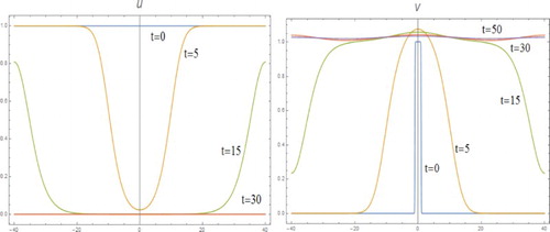
Figure 2 is the result of computation of m=2 with the other conditions same as the above case. The reaction again starts from the central region and spread out with the estimated speed of $2.5\sqrt{D}/3$, before v becomes very flat, approaching 1 as time $t\gg 1$.

Figure 2. System (II) with m=2 and D=2.

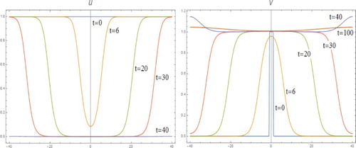
Figure 3 is the result of computation of m=2 and D=4 with other conditions same as the above case. The reaction again starts from the central region and spread out with the estimated speed of $2.5\sqrt{D}/3$, before v becomes very flat, approaching 1 as time $t\gg 1$.

Figure 3. System (II) with m=2 and D=4.

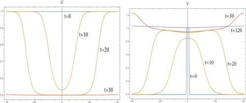
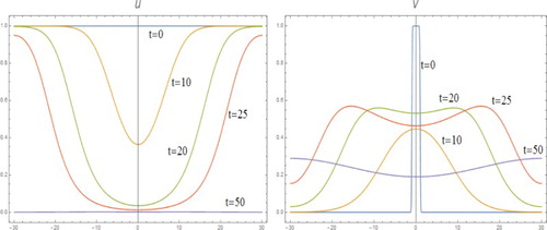
Figure 4 is the result of computation of m=1 and D=3 with initial condition of v to be $v(x,0)=\frac{\pi }{2}\sin \left(\frac{\pi }{100}\right(50+x\left)\right),-50<x<50$ and the spatial domain is $[-50,50]$. The reaction again starts from the central region and spread out with the estimated speed of in the range of $7\sqrt{D}/12<c<3\sqrt{D}/4$, (with other values of D>1 also computed to confirm the range). But instead of converging to 1, v converges to a fixed bell-shaped profile as time $t\gg 1$. In addition, u becomes two-hump from the initial one-hump and keep the same profile with diminished height as t increases before eventually tending to zero.

Figure 4. System (II) with m=1 and D=3.

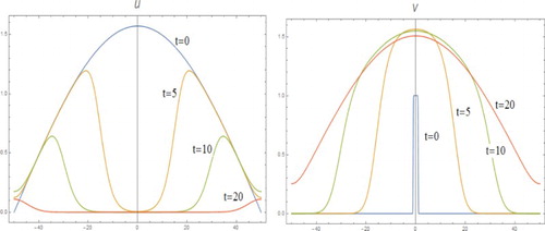
Figure 5 is the result of computation of m=2 and D=3 with other conditions same as the above case. The solutions demonstrate the same kind of qualitative behaviour as the above case except the speed range is in $7\sqrt{D}/12<c<5\sqrt{D}/6$.

Figure 5. System (II) with m=2 and D=3.

We also did some computation on (I) with the results shown in the figures below.

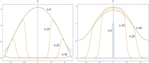
In Figures 6– 8, we present some computational results on (I) with m=2, l=1, D=4 and the same initial conditions as for various cases of (II). They show that when $k=1$ and k=0.2, the decay is very strong and v tends to zero very fast before any pattern to form effectively. But, for k=0.05, v undergoes some very interesting evolution before decay to zero eventually.

Figure 6. System (I) with m=2, l=1, D=4 and k=1.

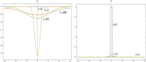
Figure 7. System (I) with m=2, l=1, D=4 and k=0.2.

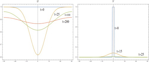
Figure 8. System (I) with m=2, l=1, D=4 and k=0.05.

Acknowledgments

The authors thank Junping Shi and Xiaoqiang Zhao for stimulating discussions.

Disclosure statement

No potential conflict of interest was reported by the authors.

References

- D.G. Aronson and H.F. Weinberger, Multidimensional nonlinear diffusion arising in population genetics, Adv. Math. 30 (1978), pp. 33–76. doi: 10.1016/0001-8708(78)90130-5
- P.W. Bates, P.C. Fife, X.F. Ren, and X.F. Wang, Traveling waves in a convolution model for phase transitions, Arch. Rational Mech. Anal. 138 (1997), pp. 105–136. doi: 10.1007/s002050050037
- J. Bricmont, A. Kupiainen, and J. Xin, Global large time self-similarity of a thermal-diffusiive combustion system with critical nonlinearity, J. Differ. Equ. 130 (1996), pp. 9–35. doi: 10.1006/jdeq.1996.0130
- X. Chen and Y. Qi, Sharp estimates on minimum travelling wave speed of reaction diffusion systems modelling autocatalysis, SIAM J. Math. Anal. 39 (2007), pp. 437–448. doi: 10.1137/060665749
- X. Chen and Y. Qi, Propagation of local disturbances in reaction diffusion systems modeling quadratic autocatalysis, SIAM J. Appl. Math. 69 (2008), pp. 273–282. doi: 10.1137/07070276X
- X. Chen, Y. Qi, and Y. Zhang, Existence of traveling waves of auto-catalytic systems with decay, J. Differ. Equ. 260 (2016), pp. 7982–7999. doi: 10.1016/j.jde.2016.02.009
- A. Doelman, R.A. Gardner, and T.J. Kaper, Stability analysis of singular patterns in the 1-D Gray-Scott model: A matched asymptotics approach, Phys. D 122 (1998), pp. 1–36. doi: 10.1016/S0167-2789(98)00180-8
- A. Doelman, W. Eckhaus, and T.J. Kaper, Slowly modulated two-pulse solutions in the Gray-Scott model II: Geometric theory, bifurcations, and splitting dynamics, SIAM J. Appl. Math. 61 (2001), pp. 2036–2062. doi: 10.1137/S0036139900372429
- S.-C . Fu and J.-C . Tsai, The evolution of traveling waves in a simple isothermal chemical system modeling quadratic autocatalysis with strong decay, J. Differ. Equ. 256 (2014), pp. 3335–3364. doi: 10.1016/j.jde.2014.02.009
- P. Gray and S.K. Scott, Autocatalytic reactions in the isothermal, continuous stirred tank reactor: Oscillations and instabilities in the system A+2B→3B, B→C, Chem. Eng. Sci. 39 (1984), pp. 1087–1097. doi: 10.1016/0009-2509(84)87017-7
- T. Kolokolnikov, M.J. Ward, and J.C. Wei, The existence and stability of spike equilibria in the one-dimensional Gray-Scott model: The pulse-splitting regime, Phys. D 202 (2005), pp. 258–293. doi: 10.1016/j.physd.2005.02.009
- Y. Li and Y.P. Wu, Stability of traveling front solutions with algebraic spatial decay for some autocatalytic chemical reaction systems, SIAM J. Math. Anal 44 (2012), pp. 1474–1521. doi: 10.1137/100814974
- K.-J. Lin, W.D. McCormick, J.E. Pearson, and H.L. Swinney, Experimental observation of self-replicating spots in a reaction-diffusion system, Nature 369 (1994), pp. 215–218. doi: 10.1038/369215a0
- J.E. Pearson, Complex patterns in a simple system, Science 261 (1993), pp. 189–192. doi: 10.1126/science.261.5118.189
- Y. Qi, et al., Multiple-Peak Traveling Waves of the Gray-Scott Model, in preparation.
- J. Shi and X. Wang, Hair-triggered instability of radial steady states, spread and extinction in semilinear heat equations, J. Differ. Equ. 231 (2006), pp. 235–251. doi: 10.1016/j.jde.2006.06.008
- H.L. Smith and X.-Q . Zhao, Dynamics of a periodically pulsed bio-reactor model, J. Differ. Equ. 155 (1999), pp. 368–404. doi: 10.1006/jdeq.1998.3587
- A.N. Zaikin and A.M. Zhabotinskii, Concentration wave propagation in two-dimensional liquid-phase self-organising systems, Nature 225 (1970), pp. 535–537. doi: 10.1038/225535b0
- Y. Zhao, Y. Wang, and J. Shi, Steady states and dynamics of an autocatalytic chemical reaction model with decay, J. Differ. Equ. 253 (2012), pp. 533–552. doi: 10.1016/j.jde.2012.03.018
- Z. Zheng, X. Chen, Y. Qi, and S. Zhou, Existence of Traveling Waves of General Gray-Scott Models, preprint.
- J. Zhou and J. Shi, Qualitative analysis of an autocatalytic chemical reaction model with decay, Proc. R. Soc. Edinburgh Sect. A 144 (2014), pp. 427–446. doi: 10.1017/S0308210512001667