Existence and uniqueness for a coupled PDE model for motor-induced microtubule organization

ABSTRACT

Microtubules (MTs) are protein filaments that provide structure to the cytoskeleton of cells and a platform for the movement of intracellular substances. The spatial organization of MTs is crucial for a cell's form and function. MTs interact with a class of proteins called motor proteins that can transport and position individual filaments, thus contributing to overall organization. In this paper, we study the mathematical properties of a coupled partial differential equation (PDE) model, introduced by White et al. in 2015, that describes the motor-induced organization of MTs. The model consists of a nonlinear coupling of a hyperbolic PDE for bound motor proteins, a parabolic PDE for unbound motor proteins, and a transport equation for MT dynamics. We locally smooth the motor drift velocity in the equation for bound motor proteins. The mollification is not only critical for the analysis of the model, but also adds biological realism. We then use a Banach Fixed Point argument to show local existence and uniqueness of mild solutions. We highlight the applicability of the model by showing numerical simulations that are consistent with in vitro experiments.

KEYWORDS:

• Microtubule asters
• vortices
• mitotic spindle
• transport equations
• reaction-diffusion systems

AMS SUBJECT CLASSIFICATION:

• 92B05
• 35M10
• 35Q92

1. Introduction

All eukaryotic cells contain a cytoskeleton. The cytoskeleton is comprised of three main protein filaments: microtubules (MTs), actin, and intermediate filaments (IFs). The cytoskeleton, as the name suggests, acts as the skeleton for a cell. The filaments of the cytoskeleton are similar between various cell types. However, the structure, function, and overall organization of the cytoskeleton are different depending on cell type, as well as cell-cycle stage. One of the primary roles of the cytoskeleton is to help cells maintain shape and internal organization, providing mechanical support that enables cells to carry out essential functions, like division and movement. However, the mechanism of organization for the protein filaments that make up the cytoskeleton is not completely understood, and so an in-depth study of the spatial patterning of such filaments is important.

In this paper, we focus on the mathematical properties of the model of White et al. [35], which was developed to study the qualitative and quantitative features of patterns formed by one of the three main cytoskeletal components, MTs. In particular, we give a novel existence and uniqueness result for the model. The model consists of a nonlinear coupling of three partial differential equations (PDEs). The first equation is of hyperbolic type (Equation (1a(1b) $\begin{array}{rl}\frac{\mathrm{\partial }{m}_{\mathrm{u}}}{\mathrm{\partial }t}-D_{\mathrm{u}}{\mathrm{\Delta }}_{\mathrm{x}}{m}_{\mathrm{u}}& =-k_{\mathrm{on}}\left(\tilde{p}\right)m_{\mathrm{u}}+k_{\mathrm{off}}{m}_{\mathrm{b}}.\end{array}$(1b) )), the second equation is parabolic (Equation (1b(2) $\frac{\mathrm{\partial }p}{\mathrm{\partial }t}+\gamma \theta \cdot {\mathrm{\nabla }}_{\mathrm{x}}p=-\lambda \left(m_{\mathrm{b}}\right)p+\lambda \left(m_{\mathrm{b}}\right){\int }_{{\mathbb{S}}^{n-1}}k(m_{\mathrm{b}},\theta ,\tilde{\theta })p(x,t,\tilde{\theta })\mathrm{d}\tilde{\theta }.$(2) )), and the third is a transport equation (Equation (2(3) ${\mathbf{\text{v}}}_{\mathbf{\text{b}}}\left(p\right)=v_{{\mathrm{b}}_{\max }}{\int }_{{\mathbb{S}}^{n-1}}\theta p(x,t,\theta )\mathrm{d}\theta .$(3) )). Each type of equation has its specific properties. For example, hyperbolic models transport discontinuities and they can form shocks [3], parabolic models regularize [4], and transport equations are also hyperbolic but they regularize moments [5]. Together they form a complex mathematical model, and the formulation of a suitable solution theory is not trivial.

For completeness, we first give a brief introduction of the other two main cytoskeletal components, actin, and IFs, in Section 1.1. Here we suggest that, in some cases, actin can be modelled in a similar fashion as MTs. Then, in Section 1.2, we give a detailed description of the components involved in MT organization and we briefly review other mathematical models for MT patterning. Lastly, in Section 1.3, we give a brief outline of the main components of the paper.

1.1. A brief introduction to cytoskeletal filaments: MTs, Actin, and IFs

MTs, which form cylindrical structures comprised of tubulin subunits, are the largest of the three protein filaments (approximately 25 nm in diameter). MTs are important in providing structural stability for the cell, as well as aiding in cell division and cell movement. Actin filaments, which are formed from actin monomers, are the smallest of the three filament types (approximately 6 nm in diameter). Actin is generally located directly under the cortex of cells, providing the mechanical scaffold needed to produce a cleavage furrow during cell division, and aiding in muscle contraction. IFs have an intermediate size (approximately 10 nm in diameter), and are comprised of various protein types. Unlike MTs and actin, the function of IFs is not as well understood, however, it is known that their disruption can have serious consequences for normal cell development.

Both MTs and actin are similar in that they are polar, meaning that subunits preferentially associate with one end of the filament and dissociate from the other. MTs and actin both undergo a type of dynamics referred to as treadmilling [17, 31]. MT treadmilling is a chemical process that is defined as the steady-state unidirectional flux of subunits through a polymer as a result of continuous net assembly at the front end of a polymer and continuous net disassembly at the back end. The result is the directed (constant) motion of a MT towards its front end. The front and back ends of MTs are called plus and minus ends and for actin are called pointed and barbed ends. IFs are known to be very stable structures and have not been found to treadmill.

MTs and actin are also similar in that they interact with a class of proteins called motor proteins. Motor proteins are ATPases, and so are driven by the hydrolysis of adenosine triphosphate (ATP). By transforming chemical energy into work, they are able to perform a number of important functions [7]. Certain types of motor proteins can walk along either MTs or actin, and when connected to two filaments simultaneously, the motors can provide pushing and pulling forces that help to organize the filaments into various configurations. Motor proteins are, in general, polymer specific, and will walk along only one type of filament. MTs and actin can also be transported along a directed path by sliding. Sliding occurs when the cargo domain of a motor is attached to a non-moving substrate (e.g. motors that are adsorbed (stuck) to a cover-slip [27, 29]), while the motile part (the motor domain) walks along a filament. The result is the directed transport of a filament along its axis. Unlike MTs and actin, there is no consistent data to suggest that IFs associate with motor proteins. However, they do interact with many other proteins, and this interaction helps to contribute to their overall spatial organization within a cell.

The dynamic interactions between MTs and motor proteins are similar to those between actin filaments and motor proteins. The class of motor proteins that interact with actin filaments are referred to as myosin-type motors. Such actin/myosin systems have been studied both experimentally and theoretically [8, 15, 16, 22, 25]. Actin can take on many complex organizations, and such organization is crucial for normal cell function. For example, actin forms tight parallel bundles, called filopodia, at the front of fibroblasts, allowing them to migrate in the direction of a wound. Also, during muscle contraction, actin fibres form tight anti-parallel bundles. Theoretical models have been developed to better understand the patterns formed by the interactions of myosin and actin alone. For example, in [16], the authors use a Monte Carlo modelling approach to model actin movement. They consider both actin rotation (as a result of myosin II motors traversing filament pairs) as well as polymerization and depolymerization of filaments. They find that optimal motor speeds (high speeds) result in alignment of filaments, whereas depolymerization results in disorganized actin structures. Theoretical models developed to describe actin and myosin dynamics have provided useful insight into the possible mechanisms involved in actin organization. Our modelling framework for the interaction of MTs and motor proteins will incorporate some of the mechanisms from the actin-myosin models (e.g. filament rotation due to interaction with motors, as well as the effect of motor speed on filament organization).

1.2. MTs and motor proteins

MTs are dynamic protein polymers formed through the self-assembly of α-, β-tubulin dimers [11, 30]. They grow through the addition of GTP (guanosine triphosphate) -bound tubulin dimers, generally at the plus- end of the MT (the end where β-tubulin is located), and shrink through dissociation of GDP (guanosine diphosphate) -bound tubulin at this end. The minus end of the MT (the end where α-tubulin is located) is generally more stable, being capped by stabilizing proteins. Two primary types of dynamic movement that individual MTs undergo are treadmilling (as described in Section 1.1) and dynamic instability [13, 32]. Dynamic instability refers to slow growth of a MT at its plus-end, followed by fast depolymerization.

There are two main classes of MT associated motor proteins: plus-end directed kinesin motors and minus end directed dynein motors. These motor proteins have many important functions. One role is that they are able to walk along MTs (either towards their plus- end or minus end), carrying cargo (like proteins and vesicles) with them, and distributing the cargo to the appropriate locations within cells. Also, motor proteins affect MT organization by helping to align MTs parallel with one another as they cross-link adjacent MTs [18, 19, 26]. As motors walk along the cross-linked MTs simultaneously, they produce pushing and pulling forces that help to reorient the MTs. Finally, as stated in Section 1.1, motors immobilized at their cargo domains can attach to a single MT and slide it along a directed path.

Similar to actin, MTs can take on many different organizations within a cell, where each particular organization is directly connected to the cellular processes that a cell is carrying out. For example, during cell division, MTs form two asters centred at the replicated centrosomes of a cell, separated by a tight anti-parallel bundle of MTs at the cell's centre, called the mitotic spindle (examples of these patterns are shown in Figure 1). Other examples of cellular processes, where MT organization plays a key role, are cell motility and cell polarization. For these processes to be carried out, many other cellular components besides motor proteins contribute to MT organization. However, when MTs interact with only motor proteins in vitro, they form a variety of patterns, including asters, vortices, and bundles (see Figure 1) [18, 19, 26]. Theoretical modelling of MT/motor systems has provided insight into the particular mechanisms required for MT pattern formation [1, 9, 12, 14, 34, 35]. In particular, such studies have shown that motor speed, directionality, processivity, as well as density, contribute to the types of MT patterns that can form.

Figure 1. Schematic of examples of MT organization in vivo and in vitro. In vivo organizations include (a) an aster with minus ends at the centre (typical of a centrosomal configuration found in non-dividing cells and moving cells), (b) an anti-parallel bundle (similar to the mitotic spindle of typical dividing cell), (c) parallel bundles (similar to those found along the axon of a neuron), and (d) mixed polarity bundles (similar to those found in plant cells). In vitro examples include those described in (a), (b), (c), and (d), but also include (e) vortices, and (f) an aster with plus-ends at the centre. Figure modified from [35].

Some of the previous models of MT organization are local-type models and include coupled reaction-diffusion equations to describe the dynamic interactions between motors and MTs [12, 14]. Such models have been studied extensively and a theoretical framework for existence and uniqueness is well established [23]. Also, under certain simplified assumptions, explicit solutions to such models exist [14]. In this study, we analyse the model for MT/motor dynamics as described in [33, 35], where MT movement is modelled using a non-local transport equation, and motor protein interaction is accounted for by coupling the transport equation to a system of reaction-diffusion equations. A non-local model describing MT movement, which implicitly incorporates motor protein movement, has been analysed using energy methods [1, 2]. Also, a simplification of the model studied here (where motor proteins are fixed in space) was analysed in [34]. For such a simplified system, semi-group methods can be applied to prove existence and uniqueness [21].

1.3. Outline of main results

In Section 2, we introduce our MT model given by Equations (1(1b) $\begin{array}{rl}\frac{\mathrm{\partial }{m}_{\mathrm{u}}}{\mathrm{\partial }t}-D_{\mathrm{u}}{\mathrm{\Delta }}_{\mathrm{x}}{m}_{\mathrm{u}}& =-k_{\mathrm{on}}\left(\tilde{p}\right)m_{\mathrm{u}}+k_{\mathrm{off}}{m}_{\mathrm{b}}.\end{array}$(1b) a), (1b(2) $\frac{\mathrm{\partial }p}{\mathrm{\partial }t}+\gamma \theta \cdot {\mathrm{\nabla }}_{\mathrm{x}}p=-\lambda \left(m_{\mathrm{b}}\right)p+\lambda \left(m_{\mathrm{b}}\right){\int }_{{\mathbb{S}}^{n-1}}k(m_{\mathrm{b}},\theta ,\tilde{\theta })p(x,t,\tilde{\theta })\mathrm{d}\tilde{\theta }.$(2) ), and (2(3) ${\mathbf{\text{v}}}_{\mathbf{\text{b}}}\left(p\right)=v_{{\mathrm{b}}_{\max }}{\int }_{{\mathbb{S}}^{n-1}}\theta p(x,t,\theta )\mathrm{d}\theta .$(3) ). The main existence and uniqueness result of the paper is developed in Section 3. Here we define the notion of a mild solution (Definition 3.1) for this system of mixed PDEs and we use a Banach Fixed Point argument to prove local existence and uniqueness of mild solutions. The mathematical analysis necessitates a regularizing assumption which we include as spatial averaging of the motor drift velocity ${\mathbf{\text{v}}}_{\mathbf{\text{b}}}$ in (5(6) $\frac{\mathrm{d}x\left(s\right)}{\mathrm{d}s}={\mathbf{\text{v}}}_b^{\epsilon }\left(p\right(x\left(s\right),s,\theta \left)\right).$(6) ). This assumption is not only critical for the mathematical analysis, it also adds realism to the model. The model describes motor densities and filament densities, hence local irregularities in the average filament orientation are averaged by the presence of many motors and many filaments. Thus an averaged velocity is biologically reasonable. In Section 4, we show numerical simulations that describe the formation of various MT patterns that are consistent with in vitro experiments [19]. We close with a discussion about biological significance and mathematical challenges.

2. A continuous model of MT dynamics

In this section, we develop our model of MT dynamics, which is based on a model originally described in [33, 35]. The primary difference in the model discussed in this paper is the definition of motor movement along MTs. In [33, 35], the direction of motor movement was assumed to be only along the average direction of MTs. Here we make the more biologically reasonable assumption that the direction of motor movement can take on a range of values, according to a normal distribution centred about the mean MT direction. Since it is likely that some MTs will be pointed away from the mean orientation and not perfectly aligned, we allow bound motor proteins to travel in directions other than the mean orientation.

We incorporate the following basic assumptions in the construction of the model: (i) motors bound to MTs move along them at some constant speed, (ii) motors can detach from MTs at some constant rate and then freely diffuse, and (iii) MTs undergo directed transport by treadmilling (although sliding can be an alternate mechanism for directed transport), and MTs are realigned to the local mean MT orientation in the presence of attached motors. We track the dynamics of the following variables in space ($x\in {\mathbb{R}}^n$), time (t>0), and orientation ($\theta \in {\mathbb{S}}^{n-1}$): $\begin{array}{rlrl}& & m_b(x,t)\text{[mass/volume]}& \text{Bound motor density};\\ & & m_u(x,t)\text{[mass/volume]}& \text{Unbound motor density};\\ & & p(x,t,\theta )\text{[mass/volume]}& \text{MT density of plus ends}.\end{array}$

2.1. Equations for motor protein dynamics

The equations for motor proteins are as follows: (1a) $\begin{array}{rl}\frac{\mathrm{\partial }{m}_{\mathrm{b}}}{\mathrm{\partial }t}+{\mathrm{\nabla }}_x\cdot \left({\mathbf{\text{v}}}_{\mathbf{\text{b}}}^{\epsilon }{m}_{\mathrm{b}}\right)& =k_{\mathrm{on}}\left(\tilde{p}\right)m_{\mathrm{u}}-k_{\mathrm{off}}{m}_{\mathrm{b}},\end{array}$(1a) (1b) $\begin{array}{rl}\frac{\mathrm{\partial }{m}_{\mathrm{u}}}{\mathrm{\partial }t}-D_{\mathrm{u}}{\mathrm{\Delta }}_{\mathrm{x}}{m}_{\mathrm{u}}& =-k_{\mathrm{on}}\left(\tilde{p}\right)m_{\mathrm{u}}+k_{\mathrm{off}}{m}_{\mathrm{b}}.\end{array}$(1b) Motor proteins exchange between a bound state $m_{\mathrm{b}}$, in which they move along MTs with velocity ${\mathbf{\text{v}}}_{\mathbf{\text{b}}}^{\epsilon }$ (defined in (5(6) $\frac{\mathrm{d}x\left(s\right)}{\mathrm{d}s}={\mathbf{\text{v}}}_b^{\epsilon }\left(p\right(x\left(s\right),s,\theta \left)\right).$(6) ) below), and an unbound state $m_{\mathrm{u}}$, in which they diffuse freely in the cytoplasm at the rate $D_{\mathrm{u}}$. Bound motors dissociate from MTs at the rate $k_{\mathrm{off}}$ while unbound motors bind to MTs at the rate $k_{\mathrm{on}}\left(\tilde{p}\right)$, where $\tilde{p}$ is the total MT density at each point in space and time (for details, see Assumptions (A1) in Section 3).

2.2. Equation for MT dynamics

We model MT dynamics with a transport equation: (2) $\frac{\mathrm{\partial }p}{\mathrm{\partial }t}+\gamma \theta \cdot {\mathrm{\nabla }}_{\mathrm{x}}p=-\lambda \left(m_{\mathrm{b}}\right)p+\lambda \left(m_{\mathrm{b}}\right){\int }_{{\mathbb{S}}^{n-1}}k(m_{\mathrm{b}},\theta ,\tilde{\theta })p(x,t,\tilde{\theta })\mathrm{d}\tilde{\theta }.$(2) The second term on the left-hand side of Equation (2(3) ${\mathbf{\text{v}}}_{\mathbf{\text{b}}}\left(p\right)=v_{{\mathrm{b}}_{\max }}{\int }_{{\mathbb{S}}^{n-1}}\theta p(x,t,\theta )\mathrm{d}\theta .$(3) ) describes treadmilling. In particular, it describes directed transport of MTs along their axis θ at a constant speed γ. The term on the right-hand side of Equation (2(3) ${\mathbf{\text{v}}}_{\mathbf{\text{b}}}\left(p\right)=v_{{\mathrm{b}}_{\max }}{\int }_{{\mathbb{S}}^{n-1}}\theta p(x,t,\theta )\mathrm{d}\theta .$(3) ) describes a velocity jump process for reorientation of MTs in the presence of motor proteins. The first term on the right-hand side of Equation (2(3) ${\mathbf{\text{v}}}_{\mathbf{\text{b}}}\left(p\right)=v_{{\mathrm{b}}_{\max }}{\int }_{{\mathbb{S}}^{n-1}}\theta p(x,t,\theta )\mathrm{d}\theta .$(3) ) represents MT reorientation away from angle θ, while the second term represents MT reorientation towards angle θ. The function $\lambda \left(m_{\mathrm{b}}\right)$ describes the rate of MT switching and the integral kernel $k(m_{\mathrm{b}},\theta ,\tilde{\theta })$ denotes the probability density of a directional switch from $\tilde{\theta }$ to θ according to a Poisson process (for details, see Assumptions (A1) in Section 3).

2.3. Equation for bound motor velocity ${\mathbf{\text{v}}}_{\mathrm{b}}^{\epsilon }$

The definition of bound motor velocity ${\mathbf{\text{v}}}_{\mathrm{b}}^{\epsilon }$ chosen here extends the choice made in the original model in [33, 35]. There it was assumed that bound motors follow the mean direction of filaments at each location, (3) ${\mathbf{\text{v}}}_{\mathbf{\text{b}}}\left(p\right)=v_{{\mathrm{b}}_{\max }}{\int }_{{\mathbb{S}}^{n-1}}\theta p(x,t,\theta )\mathrm{d}\theta .$(3) However, the mean direction of filaments can change drastically from one space point to another leading to erratic movement of individual bound motor proteins. Moreover, $m_{\mathrm{b}}$ describes a motor protein density, hence the movement velocity is an average over all individual motor velocities. To account for that, we choose a local spatial averaging over the microtubule orientations. We define the function (4) ${\varphi }_{\epsilon }\left(x\right)={\epsilon }^{-n}\varphi \left(\frac{x}{\epsilon }\right),$(4) such that $\varphi \in C^{\mathrm{\infty }}$ with compact support $[-1,1]$ and $\underset{\epsilon \to 0}{lim}{\varphi }_{\epsilon }\left(x\right)={\delta }_0\left(x\right).$ We then define the following velocity for motor proteins that takes into account variable MT orientation: (5) ${\mathbf{\text{v}}}_{\mathbf{\text{b}}}^{\epsilon }={\varphi }_{\epsilon }\ast {\mathbf{\text{v}}}_{\mathbf{\text{b}}}.$(5) In other words, bound motor proteins do not move exactly along the mean orientation as specified by ${\mathbf{\text{v}}}_{\mathbf{\text{b}}}$; for small $\epsilon$, they move in directions that are close to the mean orientation (see the discussion section for details on the role of the parameter $\epsilon$ in the existence proof).

3. Existence and uniqueness result

In this section, we describe an existence and uniqueness result for the full model given by Equations (1a(1b) $\begin{array}{rl}\frac{\mathrm{\partial }{m}_{\mathrm{u}}}{\mathrm{\partial }t}-D_{\mathrm{u}}{\mathrm{\Delta }}_{\mathrm{x}}{m}_{\mathrm{u}}& =-k_{\mathrm{on}}\left(\tilde{p}\right)m_{\mathrm{u}}+k_{\mathrm{off}}{m}_{\mathrm{b}}.\end{array}$(1b) ), (1b(2) $\frac{\mathrm{\partial }p}{\mathrm{\partial }t}+\gamma \theta \cdot {\mathrm{\nabla }}_{\mathrm{x}}p=-\lambda \left(m_{\mathrm{b}}\right)p+\lambda \left(m_{\mathrm{b}}\right){\int }_{{\mathbb{S}}^{n-1}}k(m_{\mathrm{b}},\theta ,\tilde{\theta })p(x,t,\tilde{\theta })\mathrm{d}\tilde{\theta }.$(2) ), and (2(3) ${\mathbf{\text{v}}}_{\mathbf{\text{b}}}\left(p\right)=v_{{\mathrm{b}}_{\max }}{\int }_{{\mathbb{S}}^{n-1}}\theta p(x,t,\theta )\mathrm{d}\theta .$(3) ), where we make the following assumptions on the parameter functions.

Assumptions (A1):

1. The density-dependent attachment rate $k_{\mathrm{on}}\left(\tilde{p}\right)$ is assumed to be non-negative and Lipschitz continuous with Lipschitz constant $L_{{\mathrm{k}}_{\mathrm{on}}}$. Our standard example is to use a second-order Hill function $k_{\mathrm{on}}\left(\tilde{p}\right)=k_{\mathrm{on}}^{\max }\left(\tilde{p}/(1+\tilde{p})\right)$, where $k_{\mathrm{on}}^{\max }>0$ is the maximum attachment rate and $\tilde{p}(x,t)={\int }_{{\mathbb{S}}^{n-1}}p(x,t,\theta )\mathrm{d}\theta ,$ is the total MT density at each point in space x at time t. Here, ${\mathbb{S}}^{n-1}$ denotes the $(n-1)$-dimensional unit sphere in ${\mathbb{R}}^n$. Such a description for the attachment rate suggests that motor proteins can only bind when MTs are present (i.e. $k_{\mathrm{on}}\left(0\right)=0$). Also, the association rate saturates to some finite value (i.e. $k_{\mathrm{on}}(\tilde{p}$) → $k_{\mathrm{on}}^{\max }$ as $\tilde{p}$ → ∞). Here, we assume that the saturation is due to steric interactions.

2. The turning rate $\lambda \left(m_{\mathrm{b}}\right)$ is assumed to be a non-negative and Lipschitz continuous function of the bound motor density with Lipschitz constant $L_{\lambda }$. Our standard example is $\lambda \left(m_{\mathrm{b}}\right)={\lambda }_{\max }\left(m_{\mathrm{b}}/(1+m_{\mathrm{b}})\right)$ where ${\lambda }_{\max }>0$ is the maximum switching rate. Our choice in $\lambda \left(m_{\mathrm{b}}\right)$ means that there is no switching if no bound motors are present. Also, the switching rate saturates to some maximum value ${\lambda }_{\max }$, which we assume happens due to over-crowding of motors.

3. The integral kernel $k(m_{\mathrm{b}},\theta ,\tilde{\theta })$ is a bounded, non-negative and integrable kernel that depends Lipschitz continuously on $m_{\mathrm{b}}$ with Lipschitz constant $L_k$ and it satisfies ${\int }_{{\mathbb{S}}^{n-1}}k(m_{\mathrm{b}},\theta ,\tilde{\theta })\mathrm{d}\theta =1.$ We further assume that $k(m_{\mathrm{b}},\theta ,\tilde{\theta })$ does not depend on the incoming orientation $\tilde{\theta }$, since we assume that microtubule orientation is dominated by the surrounding influences, and not by the previous orientation. This assumption could be generalized in further studies. For this choice in the integral kernel, there is a non-zero probability of orientation from any angle. A biologically realistic example for this kernel is described in Equation (33) in Section 4.

4. The constant $k_{\mathrm{off}}>0$ is the detachment rate of motors from MTs, $D_{\mathrm{u}}>0$ is the diffusion rate of unbound motors, and $\gamma >0$ is the constant treadmilling rate. For biological realism, these values must be positive.

5. For the existence result, we consider a spatial square domain Ω with periodic boundary conditions. In this case we can identify the domain with an n-dimensional torus, which we denote as ${\mathbb{T}}^n$. For a fixed time $\tau >0$, we use the notations $\mathrm{\Omega }={\mathbb{T}}^n\text{and}{Q}_{\tau }:=\mathrm{\Omega }\times [0,\tau ].$

6. We define the Banach spaces $X=L^{\mathrm{\infty }}\left(Q_{\tau }\right)\text{and}Z=L^{\mathrm{\infty }}(Q_{\tau };L^1({\mathbb{S}}^{n-1}\left)\right),$ and we consider given initial conditions $m_{\mathrm{b}}(x,0)=b\left(x\right)\in L^{\mathrm{\infty }}\left(\mathrm{\Omega }\right),m_{\mathrm{u}}(x,0)=u\left(x\right)\in L^{\mathrm{\infty }}\left(\mathrm{\Omega }\right),$ and $b\left(x\right)$ is uniformly Lipschitz continuous with constant $L_{\mathrm{b}}$ and $p(x,0,\theta )=q(x,\theta )\in L^{\mathrm{\infty }}(\mathrm{\Omega },L^1({\mathbb{S}}^{n-1}\left)\right).$

To state the main result on existence and uniqueness, we define a notion of mild solutions below. To obtain the mild solutions, we use the method of characteristics for the two hyperbolic equations (1a(1b) $\begin{array}{rl}\frac{\mathrm{\partial }{m}_{\mathrm{u}}}{\mathrm{\partial }t}-D_{\mathrm{u}}{\mathrm{\Delta }}_{\mathrm{x}}{m}_{\mathrm{u}}& =-k_{\mathrm{on}}\left(\tilde{p}\right)m_{\mathrm{u}}+k_{\mathrm{off}}{m}_{\mathrm{b}}.\end{array}$(1b) ) and (2(3) ${\mathbf{\text{v}}}_{\mathbf{\text{b}}}\left(p\right)=v_{{\mathrm{b}}_{\max }}{\int }_{{\mathbb{S}}^{n-1}}\theta p(x,t,\theta )\mathrm{d}\theta .$(3) ), and a variation of constants formula for the diffusion equation (1b(2) $\frac{\mathrm{\partial }p}{\mathrm{\partial }t}+\gamma \theta \cdot {\mathrm{\nabla }}_{\mathrm{x}}p=-\lambda \left(m_{\mathrm{b}}\right)p+\lambda \left(m_{\mathrm{b}}\right){\int }_{{\mathbb{S}}^{n-1}}k(m_{\mathrm{b}},\theta ,\tilde{\theta })p(x,t,\tilde{\theta })\mathrm{d}\tilde{\theta }.$(2) ).

For a given function $p(x,t,\theta )$, the characteristic equation of the hyperbolic equation (1a(1b) $\begin{array}{rl}\frac{\mathrm{\partial }{m}_{\mathrm{u}}}{\mathrm{\partial }t}-D_{\mathrm{u}}{\mathrm{\Delta }}_{\mathrm{x}}{m}_{\mathrm{u}}& =-k_{\mathrm{on}}\left(\tilde{p}\right)m_{\mathrm{u}}+k_{\mathrm{off}}{m}_{\mathrm{b}}.\end{array}$(1b) ) is given by (6) $\frac{\mathrm{d}x\left(s\right)}{\mathrm{d}s}={\mathbf{\text{v}}}_b^{\epsilon }\left(p\right(x\left(s\right),s,\theta \left)\right).$(6) We denote the unique solution that goes through $(x,t)$ as (7) $\alpha (s;x,t)\text{such that}\alpha (t;x,t)=x\text{and the anchor point is}{\alpha }_0=\alpha (0;x,t).$(7) Using this characteristic, we define a semigroup that is generated by the shift and decay terms of (1a(1b) $\begin{array}{rl}\frac{\mathrm{\partial }{m}_{\mathrm{u}}}{\mathrm{\partial }t}-D_{\mathrm{u}}{\mathrm{\Delta }}_{\mathrm{x}}{m}_{\mathrm{u}}& =-k_{\mathrm{on}}\left(\tilde{p}\right)m_{\mathrm{u}}+k_{\mathrm{off}}{m}_{\mathrm{b}}.\end{array}$(1b) ): (8) $\mathrm{\Lambda }\left(\alpha \right(\cdot ;x,t),t)=\exp \left(-{\int }_0^t(k_{\mathrm{off}}+\mathrm{\nabla }\cdot {\mathbf{\text{v}}}_{\mathbf{\text{b}}}^{\epsilon }(p\left(\alpha \right(s;x,t),s,\theta ))\mathrm{d}s\right).$(8)

The characteristic of the transport equation (2(3) ${\mathbf{\text{v}}}_{\mathbf{\text{b}}}\left(p\right)=v_{{\mathrm{b}}_{\max }}{\int }_{{\mathbb{S}}^{n-1}}\theta p(x,t,\theta )\mathrm{d}\theta .$(3) ) is given by $\frac{\mathrm{d}x\left(s\right)}{\mathrm{d}s}=\gamma \theta .$ We denote the unique solution that goes through $(x,t)$ with $\beta (s;x,t)\text{such that}\beta (t;x,t)=x\text{and the anchor point is}{\beta }_0=\beta (0;x,t).$ We can explicitly solve for β, namely (9) $\beta (s;x,t)=x-\gamma \theta (t-s),{\beta }_0=x-\gamma \theta t.$(9) Using the loss term in the transport model (2(3) ${\mathbf{\text{v}}}_{\mathbf{\text{b}}}\left(p\right)=v_{{\mathrm{b}}_{\max }}{\int }_{{\mathbb{S}}^{n-1}}\theta p(x,t,\theta )\mathrm{d}\theta .$(3) ), we define a multiplier (10) $\mathrm{\Pi }\left(\beta \right(\cdot ;x,t),t)=\exp \left(-{\int }_0^t\lambda \left(m_b\right(\beta (s;x,t),s\left)\right)\mathrm{d}s\right).$(10) Lastly, we denote the heat equation semigroup as $\exp \left(t{D}_u\mathrm{\Delta }\right)$.

Definition 3.1

A mild solution of the equations (1a(1b) $\begin{array}{rl}\frac{\mathrm{\partial }{m}_{\mathrm{u}}}{\mathrm{\partial }t}-D_{\mathrm{u}}{\mathrm{\Delta }}_{\mathrm{x}}{m}_{\mathrm{u}}& =-k_{\mathrm{on}}\left(\tilde{p}\right)m_{\mathrm{u}}+k_{\mathrm{off}}{m}_{\mathrm{b}}.\end{array}$(1b) ), (1b(2) $\frac{\mathrm{\partial }p}{\mathrm{\partial }t}+\gamma \theta \cdot {\mathrm{\nabla }}_{\mathrm{x}}p=-\lambda \left(m_{\mathrm{b}}\right)p+\lambda \left(m_{\mathrm{b}}\right){\int }_{{\mathbb{S}}^{n-1}}k(m_{\mathrm{b}},\theta ,\tilde{\theta })p(x,t,\tilde{\theta })\mathrm{d}\tilde{\theta }.$(2) ), and (2(3) ${\mathbf{\text{v}}}_{\mathbf{\text{b}}}\left(p\right)=v_{{\mathrm{b}}_{\max }}{\int }_{{\mathbb{S}}^{n-1}}\theta p(x,t,\theta )\mathrm{d}\theta .$(3) ) is a tuple $(m_b,m_u,p)\in X\times X\times Z$ that satisfies the following equations: $\begin{array}{rl}{m}_{\mathrm{b}}(x,t)& =b\left({\alpha }_0\right)\mathrm{\Lambda }\left(\alpha \right(\cdot ;x,t),t)+{\int }_0^t\mathrm{\Lambda }\left(\alpha \right(\cdot ;x,t),t-s)k_{\mathrm{on}}\left(\tilde{p}\right(\alpha (s;x,t),s\left)\right)\\ & \times m_{\mathrm{u}}\left(\alpha \right(s;x,t),s)\mathrm{d}s,\\ m_{\mathrm{u}}(x,t)& =\exp \left(t{D}_{\mathrm{u}}\mathrm{\Delta }\right)u\left(x\right)+{\int }_0^t\exp \left(\right(t-s\left)D_{\mathrm{u}}\mathrm{\Delta }\right)[-k_{\mathrm{on}}(\tilde{p}(x,s)\left)m_{\mathrm{u}}\right(x,s)\\ & +k_{\mathrm{off}}{m}_{\mathrm{b}}(x,s)]\mathrm{d}s\\ p(x,t,\theta )& =\mathrm{\Pi }\left(\beta \right(\cdot ;x,t),t)q(x-\gamma \theta t)+{\int }_0^t\mathrm{\Pi }\left(\beta \right(\cdot ;x,t),t-s)\lambda \left(m_{\mathrm{b}}\right(\beta (s;x,t),s\left)\right)\\ & \times k\left(m_{\mathrm{b}}\right(\beta (s;x,t),s),\theta )\tilde{p}\left(\beta \right(s;x,t),s)\mathrm{d}s,\end{array}$ where $\alpha ,\mathrm{\Lambda },\beta ,\mathrm{\Pi }$ are defined in (7(8) $\mathrm{\Lambda }\left(\alpha \right(\cdot ;x,t),t)=\exp \left(-{\int }_0^t(k_{\mathrm{off}}+\mathrm{\nabla }\cdot {\mathbf{\text{v}}}_{\mathbf{\text{b}}}^{\epsilon }(p\left(\alpha \right(s;x,t),s,\theta ))\mathrm{d}s\right).$(8) ), (8(9) $\beta (s;x,t)=x-\gamma \theta (t-s),{\beta }_0=x-\gamma \theta t.$(9) ), (9(10) $\mathrm{\Pi }\left(\beta \right(\cdot ;x,t),t)=\exp \left(-{\int }_0^t\lambda \left(m_b\right(\beta (s;x,t),s\left)\right)\mathrm{d}s\right).$(10) ), and (10(11) $\frac{\mathrm{\partial }{m}_{\mathrm{b}}^{\ast }(x,t)}{\mathrm{\partial }t}+\mathrm{\nabla }\cdot \left({\mathbf{\text{v}}}_{\mathbf{\text{b}}}^{\epsilon }\right(p\left)m_{\mathrm{b}}^{\ast }\right(x,t\left)\right)=k_{\mathrm{on}}\left(\tilde{p}\right)m_{\mathrm{u}}(x,t)-k_{\mathrm{off}}{m}_{\mathrm{b}}^{\ast }(x,t),$(11) ), respectively.

Theorem 3.2.

Assume the six assumptions in $\left(A1\right)$. There exists a $\tau >0$ such that there exists a unique mild solution $(m_b,m_u,p)$ of (1a(1b) $\begin{array}{rl}\frac{\mathrm{\partial }{m}_{\mathrm{u}}}{\mathrm{\partial }t}-D_{\mathrm{u}}{\mathrm{\Delta }}_{\mathrm{x}}{m}_{\mathrm{u}}& =-k_{\mathrm{on}}\left(\tilde{p}\right)m_{\mathrm{u}}+k_{\mathrm{off}}{m}_{\mathrm{b}}.\end{array}$(1b) ), (1b(2) $\frac{\mathrm{\partial }p}{\mathrm{\partial }t}+\gamma \theta \cdot {\mathrm{\nabla }}_{\mathrm{x}}p=-\lambda \left(m_{\mathrm{b}}\right)p+\lambda \left(m_{\mathrm{b}}\right){\int }_{{\mathbb{S}}^{n-1}}k(m_{\mathrm{b}},\theta ,\tilde{\theta })p(x,t,\tilde{\theta })\mathrm{d}\tilde{\theta }.$(2) ), and (2(3) ${\mathbf{\text{v}}}_{\mathbf{\text{b}}}\left(p\right)=v_{{\mathrm{b}}_{\max }}{\int }_{{\mathbb{S}}^{n-1}}\theta p(x,t,\theta )\mathrm{d}\theta .$(3) ) with $m_b\in X,$ $m_u$ $\in X$, and p $\in Z$.

Proof.

The proof is based on a Banach fixed point argument, and we give a brief outline first. The coupling of a hyperbolic equation (1a(1b) $\begin{array}{rl}\frac{\mathrm{\partial }{m}_{\mathrm{u}}}{\mathrm{\partial }t}-D_{\mathrm{u}}{\mathrm{\Delta }}_{\mathrm{x}}{m}_{\mathrm{u}}& =-k_{\mathrm{on}}\left(\tilde{p}\right)m_{\mathrm{u}}+k_{\mathrm{off}}{m}_{\mathrm{b}}.\end{array}$(1b) ), a parabolic equation (1b(2) $\frac{\mathrm{\partial }p}{\mathrm{\partial }t}+\gamma \theta \cdot {\mathrm{\nabla }}_{\mathrm{x}}p=-\lambda \left(m_{\mathrm{b}}\right)p+\lambda \left(m_{\mathrm{b}}\right){\int }_{{\mathbb{S}}^{n-1}}k(m_{\mathrm{b}},\theta ,\tilde{\theta })p(x,t,\tilde{\theta })\mathrm{d}\tilde{\theta }.$(2) ), and a transport equation (2(3) ${\mathbf{\text{v}}}_{\mathbf{\text{b}}}\left(p\right)=v_{{\mathrm{b}}_{\max }}{\int }_{{\mathbb{S}}^{n-1}}\theta p(x,t,\theta )\mathrm{d}\theta .$(3) ) leads to interesting mathematical challenges. We address those by using the appropriate estimates for each type of equation separately. We define four maps between the Banach spaces X and Z as follows: $\begin{array}{rl}\mathbf{\text{A}}:& X\times Z⟶X\\ & (m_{\mathrm{u}},p)\mapsto m_{\mathrm{b}},\\ \mathbf{\text{B}}:& X\times Z⟶X\\ & (m_{\mathrm{b}},p)\mapsto m_{\mathrm{u}},\\ \mathbf{\text{C}}:& X⟶Z\\ & m_{\mathrm{b}}\mapsto p,\\ \mathbf{\text{T}}:& X⟶X\\ & m_{\mathrm{b}}\mapsto \mathbf{\text{T}}\left(m_{\mathrm{b}}\right)=\mathbf{\text{A}}\left(\mathbf{\text{B}}\right(m_{\mathrm{b}},\mathbf{\text{C}}\left(m_{\mathrm{b}}\right)),\mathbf{\text{C}}(m_{\mathrm{b}}\left)\right).\end{array}$

The goal is to show that $\mathbf{\text{T}}$ is a contraction in X for τ small enough ($\tau >0$). The corresponding unique fixed point of $\mathbf{\text{T}}$ is then a unique mild solution as defined above. The remainder of the proof is divided into subsections, related to the corresponding estimates. For all sections that follow, we use the common symbol c for all bounded time-independent constants that arise in the estimates, and we use an index $c_{\epsilon }$ to keep track of constants that depend on the spatial averaging parameter $\epsilon >0$.

3.1. An estimate for $m_{\mathrm{b}}$

As a first step, we derive an expression for $m_{\mathrm{b}}$. We begin by considering the case where we are given an $m_{\mathrm{u}}\in X$ and $p\in Z$ and we let $m_{\mathrm{b}}^{\ast }$ denote the unique solution to Equation (1a(1b) $\begin{array}{rl}\frac{\mathrm{\partial }{m}_{\mathrm{u}}}{\mathrm{\partial }t}-D_{\mathrm{u}}{\mathrm{\Delta }}_{\mathrm{x}}{m}_{\mathrm{u}}& =-k_{\mathrm{on}}\left(\tilde{p}\right)m_{\mathrm{u}}+k_{\mathrm{off}}{m}_{\mathrm{b}}.\end{array}$(1b) ). In particular, (11) $\frac{\mathrm{\partial }{m}_{\mathrm{b}}^{\ast }(x,t)}{\mathrm{\partial }t}+\mathrm{\nabla }\cdot \left({\mathbf{\text{v}}}_{\mathbf{\text{b}}}^{\epsilon }\right(p\left)m_{\mathrm{b}}^{\ast }\right(x,t\left)\right)=k_{\mathrm{on}}\left(\tilde{p}\right)m_{\mathrm{u}}(x,t)-k_{\mathrm{off}}{m}_{\mathrm{b}}^{\ast }(x,t),$(11) which we can rewrite as (12) $\begin{array}{rl}& \frac{\mathrm{\partial }{m}_{\mathrm{b}}^{\ast }(x,t)}{\mathrm{\partial }t}+{\mathbf{\text{v}}}_{\mathbf{\text{b}}}^{\epsilon }\left(p\right)\cdot \mathrm{\nabla }{m}_{\mathrm{b}}^{\ast }(x,t)\\ & =-(\mathrm{\nabla }\cdot {\mathbf{\text{v}}}_{\mathbf{\text{b}}}^{\epsilon }(p\left)\right)m_{\mathrm{b}}^{\ast }(x,t)+k_{\mathrm{on}}\left(\tilde{p}\right)m_{\mathrm{u}}(x,t)-k_{\mathrm{off}}{m}_{\mathrm{b}}^{\ast }(x,t).\end{array}$(12) The characteristics of (12(13) $\begin{array}{rl}& \frac{\mathrm{d}{m}_{\mathrm{b}}^{\ast }\left(\alpha \right(s;x,t\left)\right)}{\mathrm{d}s}+[k_{\mathrm{off}}+\mathrm{\nabla }\cdot {\mathbf{\text{v}}}_{\mathbf{\text{b}}}^{\epsilon }(p\left(\alpha \right(s;x,t),s,\theta ),s\left)\right]m_{\mathrm{b}}^{\ast }\left(\alpha \right(s;x,t),s)\\ & =k_{\mathrm{on}}\left(\tilde{p}\right(\alpha (s;x,t),s\left)\right)m_{\mathrm{u}}\left(\alpha \right(s;x,t),s).\end{array}$(13) ) are given by (6(7) $\alpha (s;x,t)\text{such that}\alpha (t;x,t)=x\text{and the anchor point is}{\alpha }_0=\alpha (0;x,t).$(7) ) with solution $\alpha (s;x,t)$. Then Equation (12(13) $\begin{array}{rl}& \frac{\mathrm{d}{m}_{\mathrm{b}}^{\ast }\left(\alpha \right(s;x,t\left)\right)}{\mathrm{d}s}+[k_{\mathrm{off}}+\mathrm{\nabla }\cdot {\mathbf{\text{v}}}_{\mathbf{\text{b}}}^{\epsilon }(p\left(\alpha \right(s;x,t),s,\theta ),s\left)\right]m_{\mathrm{b}}^{\ast }\left(\alpha \right(s;x,t),s)\\ & =k_{\mathrm{on}}\left(\tilde{p}\right(\alpha (s;x,t),s\left)\right)m_{\mathrm{u}}\left(\alpha \right(s;x,t),s).\end{array}$(13) ) can be written as on ordinary differential equation along characteristics: (13) $\begin{array}{rl}& \frac{\mathrm{d}{m}_{\mathrm{b}}^{\ast }\left(\alpha \right(s;x,t\left)\right)}{\mathrm{d}s}+[k_{\mathrm{off}}+\mathrm{\nabla }\cdot {\mathbf{\text{v}}}_{\mathbf{\text{b}}}^{\epsilon }(p\left(\alpha \right(s;x,t),s,\theta ),s\left)\right]m_{\mathrm{b}}^{\ast }\left(\alpha \right(s;x,t),s)\\ & =k_{\mathrm{on}}\left(\tilde{p}\right(\alpha (s;x,t),s\left)\right)m_{\mathrm{u}}\left(\alpha \right(s;x,t),s).\end{array}$(13) For given $(x,t)$ we define the anchor point ${\alpha }_0:=\alpha (0;x,t)$, which allows us to find a mild solution of (12(13) $\begin{array}{rl}& \frac{\mathrm{d}{m}_{\mathrm{b}}^{\ast }\left(\alpha \right(s;x,t\left)\right)}{\mathrm{d}s}+[k_{\mathrm{off}}+\mathrm{\nabla }\cdot {\mathbf{\text{v}}}_{\mathbf{\text{b}}}^{\epsilon }(p\left(\alpha \right(s;x,t),s,\theta ),s\left)\right]m_{\mathrm{b}}^{\ast }\left(\alpha \right(s;x,t),s)\\ & =k_{\mathrm{on}}\left(\tilde{p}\right(\alpha (s;x,t),s\left)\right)m_{\mathrm{u}}\left(\alpha \right(s;x,t),s).\end{array}$(13) ) using the integrating factor Λ from (8(9) $\beta (s;x,t)=x-\gamma \theta (t-s),{\beta }_0=x-\gamma \theta t.$(9) ) as (14) $\begin{array}{rl}{m}_{\mathrm{b}}^{\ast }(x,t)& =b\left({\alpha }_0\right)\mathrm{\Lambda }\left(\alpha \right(\cdot ;x,t),t)\\ & +{\int }_0^t\mathrm{\Lambda }\left(\alpha \right(\cdot ;x,t),t-s)k_{\mathrm{on}}\left(\tilde{p}\right(\alpha (s;x,t),s\left)\right)m_{\mathrm{u}}\left(\alpha \right(s;x,t),s)\mathrm{d}s,\end{array}$(14) where $t\in [0,\tau ]$. The velocity ${\mathbf{\text{v}}}_{\mathbf{\text{b}}}^{\epsilon }$ in (5(6) $\frac{\mathrm{d}x\left(s\right)}{\mathrm{d}s}={\mathbf{\text{v}}}_b^{\epsilon }\left(p\right(x\left(s\right),s,\theta \left)\right).$(6) ) is Lipschitz continuous in p and $\mathrm{\nabla }\cdot {\mathbf{\text{v}}}_{\mathbf{\text{b}}}^{\epsilon }\left(p\right)$ is bounded in $L^{\mathrm{\infty }}\left(Q_{\tau }\right)$. The on-rate $k_{\mathrm{on}}\left(\tilde{p}\right)$ is also Lipschitz continuous. If initial conditions for $m_{\mathrm{b}}^{\ast }$ are given as in Definition 3.1 there are constants such that $\Vert m_{\mathrm{b}}^{\ast }{\Vert }_{L^{\mathrm{\infty }}}\le c{e}^{c_{\epsilon }t}(\Vert b{\Vert }_{L^{\mathrm{\infty }}}+\Vert m_{\mathrm{u}}{\Vert }_{L^{\mathrm{\infty }}}).$ Hence for $t\in [0,\tau ]$ (14(15) $\begin{array}{rl}{m}_u^{\left(i\right)}\left(s\right)& =m_u^{\left(i\right)}\left({\alpha }^{\left(i\right)}\right(s;x,t),s)\\ {\tilde{p}}^{\left(i\right)}\left(s\right)& ={\tilde{p}}^{\left(i\right)}\left({\alpha }^{\left(i\right)}\right(s;x,t),s)\\ {\mathrm{\Lambda }}^{\left(i\right)}\left(s\right)& =\mathrm{\Lambda }\left({\alpha }^{\left(i\right)}\right(s;x,t),s)\\ k_{\mathrm{on}}^{\left(i\right)}\left(s\right)& =k_{\mathrm{on}}\left({\alpha }^{\left(i\right)}\right(s;x,t),s),\text{for}i=1,2.\end{array}$(15) ) defines a map $\begin{array}{rl}A:X\times Z& ⟶X\\ (m_{\mathrm{u}},p)& \mapsto m_{\mathrm{b}}^{\ast }.\end{array}$

To show that this map is a contraction, we use the method of characteristics again. We now consider two different inputs $(m_u^{\left(1\right)},p^{\left(1\right)})$ and $(m_u^{\left(2\right)},p^{\left(2\right)})$ and consider the corresponding solutions $m_b^{\ast \left(1\right)}$ and $m_b^{\ast \left(2\right)}$. We abbreviate: (15) $\begin{array}{rl}{m}_u^{\left(i\right)}\left(s\right)& =m_u^{\left(i\right)}\left({\alpha }^{\left(i\right)}\right(s;x,t),s)\\ {\tilde{p}}^{\left(i\right)}\left(s\right)& ={\tilde{p}}^{\left(i\right)}\left({\alpha }^{\left(i\right)}\right(s;x,t),s)\\ {\mathrm{\Lambda }}^{\left(i\right)}\left(s\right)& =\mathrm{\Lambda }\left({\alpha }^{\left(i\right)}\right(s;x,t),s)\\ k_{\mathrm{on}}^{\left(i\right)}\left(s\right)& =k_{\mathrm{on}}\left({\alpha }^{\left(i\right)}\right(s;x,t),s),\text{for}i=1,2.\end{array}$(15)

Notice that, since ${\mathbf{\text{v}}}_{\mathrm{b}}^{\epsilon }$ depends on ${\tilde{p}}^{\left(i\right)}$, the characteristics ${\alpha }^{\left(1\right)}(s;x,t)$ and ${\alpha }^{\left(2\right)}(s;x,t)$ will differ. They have a common point $(x,t)$ and individual anchor points ${\alpha }_0^{\left(i\right)}={\alpha }^{\left(i\right)}(0;x,t)$, i=1,2.

Integrating both sides of the characteristic equation (6(7) $\alpha (s;x,t)\text{such that}\alpha (t;x,t)=x\text{and the anchor point is}{\alpha }_0=\alpha (0;x,t).$(7) ) with respect to s from 0 to t and taking the difference, we see that the anchor points are close for small times (16) $\begin{array}{rl}|{\alpha }_0^{\left(1\right)}-{\alpha }_0^{\left(2\right)}|& \le |{\mathbf{\text{v}}}_{\mathbf{\text{b}}}^{\epsilon }|{\int }_0^t|{\tilde{p}}^{\left(1\right)}\left(s\right)-{\tilde{p}}^{\left(2\right)}\left(s\right)|\mathrm{d}s\\ & \le |{\mathbf{\text{v}}}_{\mathbf{\text{b}}}^{\epsilon }|t\underset{0\le s\le t}{sup}|{\tilde{p}}^{\left(1\right)}\left(s\right)-{\tilde{p}}^{\left(2\right)}\left(s\right)|.\end{array}$(16) Now, we estimate the distance between two solutions $m_{\mathrm{b}}^{\ast \left(1\right)}$ and $m_{\mathrm{b}}^{\ast \left(2\right)}$ given $m_{\mathrm{u}}^{\left(i\right)},{\tilde{p}}^{\left(i\right)}\in X$ for i=1 and 2. The initial conditions $m_{\mathrm{b}}^{\left(1\right)}(x,0)=m_{\mathrm{b}}^{\left(2\right)}(x,0)=b\left(x\right)$ are Lipschitz continuous and bounded, and, using (14) and the abbreviations in (15), the two solutions are (17) $\begin{array}{rl}{m}_{\mathrm{b}}^{\ast \left(1\right)}(x,t)& ={\mathrm{\Lambda }}^{\left(1\right)}\left(t\right)b\left({\alpha }_0^{\left(1\right)}\right)+{\int }_0^t{\mathrm{\Lambda }}^{\left(1\right)}(t-s)k_{\mathrm{on}}^{\left(1\right)}\left(s\right)m_{\mathrm{u}}^{\left(1\right)}\left(s\right)\mathrm{d}s,\end{array}$(17) (18) $\begin{array}{rl}{m}_{\mathrm{b}}^{\ast \left(2\right)}(x,t)& ={\mathrm{\Lambda }}^{\left(2\right)}\left(t\right)b\left({\alpha }_0^{\left(2\right)}\right)+{\int }_0^t{\mathrm{\Lambda }}^{\left(2\right)}(t-s)k_{\mathrm{on}}^{\left(2\right)}\left(s\right)m_{\mathrm{u}}^{\left(2\right)}\left(s\right)\mathrm{d}s.\end{array}$(18)

That is, we estimate $|m_{\mathrm{b}}^{\ast \left(1\right)}(x,t)-m_{\mathrm{b}}^{\ast \left(2\right)}(x,t)|$ as $\begin{array}{rl}& |m_{\mathrm{b}}^{\ast \left(1\right)}(x,t)-m_{\mathrm{b}}^{\ast \left(2\right)}(x,t){|}_{L^{\mathrm{\infty }}}\\ & \le |{\mathrm{\Lambda }}^{\left(1\right)}\left(t\right)b\left({\alpha }_0^{\left(1\right)}\right)-{\mathrm{\Lambda }}^{\left(2\right)}\left(t\right)b\left({\alpha }_0^{\left(2\right)}\right){|}_{L^{\mathrm{\infty }}}\\ & +{\int }_0^t|{\mathrm{\Lambda }}^{\left(1\right)}(t-s)k_{\mathrm{on}}^{\left(1\right)}\left(s\right)m_{\mathrm{u}}^{\left(1\right)}\left(s\right)-{\mathrm{\Lambda }}^{\left(2\right)}(t-s)k_{\mathrm{on}}^{\left(2\right)}\left(s\right)m_{\mathrm{u}}^{\left(2\right)}\left(s\right){|}_{L^{\mathrm{\infty }}}\mathrm{d}s\\ & \le |{\mathrm{\Lambda }}^{\left(1\right)}{|}_{\mathrm{\infty }}|b\left({\alpha }_0^{\left(1\right)}\right)-b\left({\alpha }_0^{\left(2\right)}\right){|}_{\mathrm{\infty }}+|b\left({\alpha }_0^{\left(2\right)}\right){|}_{\mathrm{\infty }}|{\mathrm{\Lambda }}^{\left(1\right)}\left(t\right)-{\mathrm{\Lambda }}^{\left(2\right)}\left(t\right){|}_{\mathrm{\infty }}\\ & +{\int }_0^t|{\mathrm{\Lambda }}^{\left(1\right)}(t-s)-{\mathrm{\Lambda }}^{\left(2\right)}(t-s){|}_{\mathrm{\infty }}|k_{\mathrm{on}}^{\left(1\right)}{m}_{\mathrm{u}}^{\left(1\right)}{|}_{\mathrm{\infty }}+|{\mathrm{\Lambda }}^{\left(2\right)}{|}_{\mathrm{\infty }}|k_{\mathrm{on}}^{\left(1\right)}-k_{\mathrm{on}}^{\left(2\right)}{|}_{\mathrm{\infty }}|m_{\mathrm{u}}^{\left(1\right)}{|}_{\mathrm{\infty }}\\ & +|{\mathrm{\Lambda }}^{\left(2\right)}(t-s)k_{\mathrm{on}}^{\left(2\right)}\left(s\right)||m_{\mathrm{u}}^{\left(1\right)}-m_{\mathrm{u}}^{\left(2\right)}{|}_{\mathrm{\infty }}\mathrm{d}s\\ & \le \underset{\mathbf{\text{I}}}{\underbrace{c{L}_{\mathrm{b}}|{\alpha }_0^{\left(1\right)}-{\alpha }_0^{\left(2\right)}{|}_{\mathrm{\infty }}}}+\underset{\mathbf{\text{II}}}{\underbrace{c|{\mathrm{\Lambda }}^{\left(1\right)}\left(t\right)-{\mathrm{\Lambda }}^{\left(2\right)}\left(t\right){|}_{\mathrm{\infty }}}}\\ & +\underset{\mathbf{\text{{III}}}}{\underbrace{ct(|{\mathrm{\Lambda }}^{\left(1\right)}-{\mathrm{\Lambda }}^{\left(2\right)}{|}_{L^{\mathrm{\infty }}\left(Q_{\tau }\right)}+|k_{\mathrm{on}}^{\left(1\right)}-k_{\mathrm{on}}^{\left(2\right)}{|}_{\mathrm{\infty }}+|m_{\mathrm{u}}^{\left(1\right)}-m_{\mathrm{u}}^{\left(2\right)}{|}_{\mathrm{\infty }})}}.\end{array}$ Simplifying I: Substitution of estimate (16) into I, we obtain (19) $|{\alpha }_0^{\left(1\right)}-{\alpha }_0^{\left(2\right)}|\le |{\mathbf{\text{v}}}_{\mathbf{\text{b}}}^{\epsilon }|t|{\tilde{p}}^{\left(1\right)}-{\tilde{p}}^{\left(2\right)}{|}_{L^{\mathrm{\infty }}}.$(19)

Simplifying II: The term $|{\mathrm{\Lambda }}^{\left(1\right)}\left(t\right)-{\mathrm{\Lambda }}^{\left(2\right)}\left(t\right)|$ from II can be simplified as (20) $\begin{array}{rl}& |{\mathrm{\Lambda }}^{\left(1\right)}\left(t\right)-{\mathrm{\Lambda }}^{\left(2\right)}\left(t\right){|}_{L^{\mathrm{\infty }}}\\ & =\left|\exp \left(-{\int }_0^t[k_{\mathrm{off}}+\mathrm{\nabla }\cdot {{\mathbf{\text{v}}}_{\mathbf{\text{b}}}^{\epsilon }}^{\left(1\right)}({\alpha }^{\left(1\right)}\left(s\right)\left)\right]\mathrm{d}s)-\exp (-{\int }_0^t[k_{\mathrm{off}}+\mathrm{\nabla }\cdot {{\mathbf{\text{v}}}_{\mathbf{\text{b}}}^{\epsilon }}^{\left(2\right)}({\alpha }^{\left(2\right)}\left(s\right)\left)\right]\mathrm{d}s\right)\right|\\ & \le ct|\mathrm{\nabla }\left({{\mathbf{\text{v}}}_{\mathbf{\text{b}}}^{\epsilon }}^{\left(1\right)}\right({\alpha }^{\left(1\right)}\left(s\right))-{{\mathbf{\text{v}}}_{\mathbf{\text{b}}}^{\epsilon }}^{\left(1\right)}({\alpha }^{\left(1\right)}\left(s\right)\left)\right){|}_{L^{\mathrm{\infty }}},\\ & =ct{\left|v_{{\mathrm{b}}_{\max }}\mathrm{\nabla }{\varphi }_{\epsilon }\ast {\int }_{{\mathbb{S}}^{n-1}}\theta \left(p^{\left(1\right)}\right({\alpha }^{\left(1\right)}\left(s\right),s,\theta )-p^{\left(2\right)}({\alpha }^{\left(2\right)}\left(s\right),s,\theta \left)\right)\mathrm{d}\theta \right|}_{\mathrm{\infty }}\\ & =ct{\left|v_{{\mathrm{b}}_{\max }}\mathrm{\nabla }{\varphi }_{\epsilon }\ast {\int }_{{\mathbb{S}}^{n-1}}\theta \left(p^{\left(1\right)}\right({\alpha }^{\left(1\right)}\left(s\right),s,\theta )-p^{\left(1\right)}({\alpha }^{\left(2\right)}\left(s\right),s,\theta \left)\right)\mathrm{d}\theta \right|}_{\mathrm{\infty }}\\ & +{\left|v_{{\mathrm{b}}_{\max }}\mathrm{\nabla }{\varphi }_{\epsilon }\ast {\int }_{{\mathbb{S}}^{n-1}}\theta \left(p^{\left(1\right)}\right({\alpha }^{\left(2\right)}\left(s\right),s,\theta )-p^{\left(2\right)}({\alpha }^{\left(2\right)}\left(s\right),s,\theta \left)\right)\mathrm{d}\theta \right|}_{\mathrm{\infty }}\\ & \le c_{\epsilon }t(|{\alpha }^{\left(1\right)}-{\alpha }^{\left(2\right)}{|}_{\mathrm{\infty }}+|p^{\left(1\right)}-p^{\left(2\right)}{|}_Z),\end{array}$(20) since we know already that the exponents are bounded.

The characteristics ${\alpha }^{\left(1\right)}$ and ${\alpha }^{\left(2\right)}$ have a common point at $(x,t)$, hence we can extend the estimate (16) for each intermediate time $0\le s\le t$ as $|{\alpha }^{\left(1\right)}\left(s\right)-{\alpha }^{\left(2\right)}\left(s\right)|\le |{\mathbf{\text{v}}}_{\mathbf{\text{b}}}^{\epsilon }|(t-s)|{\tilde{p}}^{\left(1\right)}-{\tilde{p}}^{\left(2\right)}{|}_{L^{\mathrm{\infty }}}.$ By the definition of X and Z we also have that for any function $\phi \in Z$ $|\tilde{\phi }{|}_{L^{\mathrm{\infty }}}\le |\phi {|}_Z,$ hence for $t\in [0,\tau ]$, we find (21) $\mathbf{\text{II}}=c|{\mathrm{\Lambda }}^{\left(1\right)}\left(t\right)-{\mathrm{\Lambda }}^{\left(2\right)}\left(t\right){|}_{L^{\mathrm{\infty }}}|\le c_{\epsilon }t|p^{\left(1\right)}-p^{\left(2\right)}{|}_Z.$(21) Simplifying III: Based on the estimates above, we can estimate the third term $\mathbf{\text{III}}$ as $\mathbf{\text{III}}\le ct(c_{\epsilon }t|p^{\left(1\right)}-p^{\left(2\right)}{|}_Z+c{L}_{{\mathrm{k}}_{\mathrm{on}}}t|{\tilde{p}}^{\left(1\right)}-{\tilde{p}}^{\left(2\right)}{|}_X+c|m_{\mathrm{u}}^{\left(1\right)}-m_{\mathrm{u}}^{\left(2\right)}{|}_X).$ Putting $\mathbf{\text{I, II, III}}$ together, we get for $t\in [0,\tau ]$ that (22) $|m_{\mathrm{b}}^{\ast \left(1\right)}(x,t)-m_{\mathrm{b}}^{\ast \left(2\right)}(x,t){|}_{L^{\mathrm{\infty }}}\le c_{\epsilon }t(|p^{\left(1\right)}-p^{\left(2\right)}{|}_Z+|m_{\mathrm{u}}^{\left(1\right)}-m_{\mathrm{u}}^{\left(2\right)}{|}_X).$(22)

3.2. An estimate for $m_{\mathrm{u}}$

Next, we derive an expression for $m_{\mathrm{u}}$. We begin by considering the case where we are given an $m_{\mathrm{b}}\in X$ and $p\in Z$, and assume that $m_{\mathrm{u}}^{\ast }$ satisfies Equation (1b(2) $\frac{\mathrm{\partial }p}{\mathrm{\partial }t}+\gamma \theta \cdot {\mathrm{\nabla }}_{\mathrm{x}}p=-\lambda \left(m_{\mathrm{b}}\right)p+\lambda \left(m_{\mathrm{b}}\right){\int }_{{\mathbb{S}}^{n-1}}k(m_{\mathrm{b}},\theta ,\tilde{\theta })p(x,t,\tilde{\theta })\mathrm{d}\tilde{\theta }.$(2) ), That is, (23) $\frac{\mathrm{\partial }{m}_{\mathrm{u}}^{\ast }(x,t)}{\mathrm{\partial }t}-D_{\mathrm{u}}\mathrm{\Delta }{m}_{\mathrm{u}}^{\ast }(x,t)=-k_{\mathrm{on}}\left(\tilde{p}\right)m_{\mathrm{u}}^{\ast }(x,t)+k_{\mathrm{off}}{m}_{\mathrm{b}}(x,t).$(23) This is a linear parabolic equation and its solution can be written as [28] (24) $\begin{array}{rl}{m}_{\mathrm{u}}^{\ast }(x,t)& =\exp \left(t{D}_{\mathrm{u}}\mathrm{\Delta }\right)m_{\mathrm{u}}^{\ast }(x,0)\\ & +{\int }_0^t\exp \left(\right(t-s\left)D_{\mathrm{u}}\mathrm{\Delta }\right)\left[k_{\mathrm{on}}\right(\tilde{p}(x,s)\left)m_{\mathrm{u}}^{\ast }\right(x,s)+k_{\mathrm{off}}{m}_{\mathrm{b}}(x,s\left)\right]\mathrm{d}s.\end{array}$(24) Again, we estimate the distance between two solutions $m_{\mathrm{u}}^{\ast \left(1\right)}(x,t)$ and $m_{\mathrm{u}}^{\ast \left(2\right)}(x,t)$, for given $m_{\mathrm{b}}^{\left(i\right)}\in X$ and $p^{\left(i\right)}$ $\in Z$, and initial conditions $m_{\mathrm{u}}^{\left(1\right)}(x,0)=m_{\mathrm{u}}^{\left(2\right)}(x,0)=u\left(x\right)$. $\begin{array}{rl}& |m_{\mathrm{u}}^{\ast \left(1\right)}(x,t)-m_{\mathrm{u}}^{\ast \left(2\right)}(x,t){|}_{L^{\mathrm{\infty }}}\\ & =|\exp \left(t{D}_{\mathrm{u}}\mathrm{\Delta }\right)u\left(x\right)-\exp \left(t{D}_{\mathrm{u}}\mathrm{\Delta }\right)u\left(x\right)\\ & +{\int }_0^t\exp \left(\right(t-s\left)D_{\mathrm{u}}\mathrm{\Delta }\right)(k_{\mathrm{on}}^{\left(1\right)}{m}_{\mathrm{u}}^{\ast \left(1\right)}+k_{\mathrm{off}}{m}_{\mathrm{b}}^{\left(1\right)}-k_{\mathrm{on}}^{\left(2\right)}{m}_{\mathrm{u}}^{\ast \left(2\right)}+k_{\mathrm{off}}{m}_{\mathrm{b}}^{\left(2\right)})\mathrm{d}s|\\ & \le {\int }_0^t|\exp \left(\right(t-s\left)D_{\mathrm{u}}\mathrm{\Delta }\right)(k_{\mathrm{on}}^{\left(1\right)}{m}_{\mathrm{u}}^{\ast \left(1\right)}+k_{\mathrm{off}}{m}_{\mathrm{b}}^{\left(1\right)}-k_{\mathrm{on}}^{\left(2\right)}{m}_{\mathrm{u}}^{\ast \left(2\right)}+k_{\mathrm{off}}{m}_{\mathrm{b}}^{\left(2\right)}){|}_{L^{\mathrm{\infty }}}\mathrm{d}s.\end{array}$

The heat equation semigroup is a bounded linear operator on $L^{\mathrm{\infty }}\left(Q_{\tau }\right)$ [28], hence (25) $|\exp \left(t{D}_{\mathrm{u}}\mathrm{\Delta }\right)f{|}_{L^{\mathrm{\infty }}}\le c|f{|}_{L^{\mathrm{\infty }}},$(25) and we obtain $\begin{array}{rl}& |m_{\mathrm{u}}^{\ast \left(1\right)}(x,t)-m_{\mathrm{u}}^{\ast \left(2\right)}(x,t){|}_{L^{\mathrm{\infty }}}\\ & \le c{\int }_0^t(c_1|k_{\mathrm{on}}^{\left(1\right)}-k_{\mathrm{on}}^{\left(2\right)}{|}_{L^{\mathrm{\infty }}}+c_2|m_{\mathrm{u}}^{\ast \left(1\right)}-m_{\mathrm{u}}^{\ast \left(2\right)}{|}_{L^{\mathrm{\infty }}}+c_3{k}_{\mathrm{off}}|m_{\mathrm{b}}^{\left(1\right)}-m_{\mathrm{b}}^{\left(2\right)}{|}_{L^{\mathrm{\infty }}})\mathrm{d}s\\ & \le \underset{k_{\mathrm{on}}\text{is Lipschitz w.r.t}\tilde{p}}{\underbrace{ct{L}_{{\mathrm{k}}_{\mathrm{on}}}|{\tilde{p}}^{\left(1\right)}-{\tilde{p}}^{\left(2\right)}{|}_{L^{\mathrm{\infty }}}}}+ct{k}_{\mathrm{off}}|m_{\mathrm{b}}^{\left(1\right)}-m_{\mathrm{b}}^{\left(2\right)}{|}_{L^{\mathrm{\infty }}}+c{\int }_0^t|m_{\mathrm{u}}^{\ast \left(1\right)}-m_{\mathrm{u}}^{\ast \left(2\right)}{|}_{L^{\mathrm{\infty }}}\mathrm{d}s.\end{array}$ Grønwall's Lemma [23] then implies (26) $\begin{array}{rl}& |m_{\mathrm{u}}^{\ast \left(1\right)}(x,t)-m_{\mathrm{u}}^{\ast \left(2\right)}(x,t){|}_{L^{\mathrm{\infty }}}\\ & \le (ct{L}_{{\mathrm{k}}_{\mathrm{on}}}|{\tilde{p}}^{\left(1\right)}-{\tilde{p}}^{\left(2\right)}{|}_{L^{\mathrm{\infty }}}+ct{k}_{\mathrm{off}}|m_{\mathrm{b}}^{\left(1\right)}-m_{\mathrm{b}}^{\left(2\right)}{|}_{L^{\mathrm{\infty }}})\exp \left(ct\right)\\ & \le (ct{L}_{k_{\mathrm{on}}}|p^{\left(1\right)}-p^{\left(2\right)}{|}_Z+ct{k}_{\mathrm{off}}|m_{\mathrm{b}}^{\left(1\right)}-m_{\mathrm{b}}^{\left(2\right)}{|}_X)\exp \left(ct\right).\end{array}$(26) Thus, we have a continuous mapping $\mathbf{\text{B}}$ defined by $\begin{array}{rl}\mathbf{\text{B}}:X\times Z& ⟶L^{\mathrm{\infty }}\left(Q_{\tau }\right)\\ (m_{\mathrm{b}},p)& \mapsto m_{\mathrm{u}}^{\ast }.\end{array}$

3.3. An estimate for p

We derive an expression for p using Equation (2(3) ${\mathbf{\text{v}}}_{\mathbf{\text{b}}}\left(p\right)=v_{{\mathrm{b}}_{\max }}{\int }_{{\mathbb{S}}^{n-1}}\theta p(x,t,\theta )\mathrm{d}\theta .$(3) ). Here, we follow a similar method to that used by Hillen et al. [6]. Now $m_{\mathrm{u}}\in X$ and $m_{\mathrm{b}}\in X$ are given, and $p^{\ast }$ denotes the unique solution of (27) $\begin{array}{rl}& \frac{\mathrm{\partial }{p}^{\ast }(x,t,\theta )}{\mathrm{\partial }t}+\gamma \theta \cdot {\mathrm{\nabla }}_x{p}^{\ast }(x,t,\theta )\\ & =-\lambda \left(m_{\mathrm{b}}\right)p^{\ast }(x,t,\theta )+\lambda \left(m_{\mathrm{b}}\right){\int }_{{\mathbb{S}}^{n-1}}k(m_{\mathrm{b}},\theta ,\tilde{\theta })p^{\ast }(x,t,\tilde{\theta })\mathrm{d}\tilde{\theta }\\ & =-\lambda \left(m_{\mathrm{b}}\right)p^{\ast }(x,t,\theta )+\lambda \left(m_{\mathrm{b}}\right)k(m_{\mathrm{b}},\theta ){\tilde{p}}^{\ast }(x,t),\end{array}$(27) where we used the fact that the kernel $k(m_{\mathrm{b}},\theta ,\tilde{\theta })$ does not depend on the incoming orientation $\tilde{\theta }$ (see Assumptions (A1)).

This equation is a hyperbolic transport equation, which has well-defined classical solutions (see e.g.  [5, 6]), and so we can use the method of characteristics to determine an expression for p. The unique characteristic through the point $(x,t)$ is given by (9(10) $\mathrm{\Pi }\left(\beta \right(\cdot ;x,t),t)=\exp \left(-{\int }_0^t\lambda \left(m_b\right(\beta (s;x,t),s\left)\right)\mathrm{d}s\right).$(10) ) and we recall it here: (28) $\beta (s;x,t)=x-\gamma \theta (t-s),{\beta }_0=x-\gamma \theta t.$(28)

Substituting the characteristic $\beta (s;x,t)$ into Equation (27) and writing in terms of the material derivative, we arrive at (29) $\begin{array}{rl}& \frac{\mathrm{d}}{\mathrm{d}s}{p}^{\ast }(\beta (s;x,t),s,\theta )+\lambda \left(m_{\mathrm{b}}\right(\beta (s;x,t),s\left)\right)p^{\ast }(\beta (s;x,t),s,\theta )\\ & =\lambda \left(m_{\mathrm{b}}\right(\beta (s;x,t),s\left)\right)k\left(m_{\mathrm{b}}\right(\beta (s;x,t),s),\theta ){\tilde{p}}^{\ast }(\beta (s;x,t),s).\end{array}$(29)

We can solve Equation (29) by using an integrating factor (10(11) $\frac{\mathrm{\partial }{m}_{\mathrm{b}}^{\ast }(x,t)}{\mathrm{\partial }t}+\mathrm{\nabla }\cdot \left({\mathbf{\text{v}}}_{\mathbf{\text{b}}}^{\epsilon }\right(p\left)m_{\mathrm{b}}^{\ast }\right(x,t\left)\right)=k_{\mathrm{on}}\left(\tilde{p}\right)m_{\mathrm{u}}(x,t)-k_{\mathrm{off}}{m}_{\mathrm{b}}^{\ast }(x,t),$(11) ). We rewrite the integrating factor using the explicit form of the characteristics in (28) as $\mathrm{\Pi }(x,t)=\exp (-{\int }_0^t\lambda (m_{\mathrm{b}}(x-\gamma \theta (t-s),s)\left)\mathrm{d}s\right).$ Then (30) $\begin{array}{rl}& p^{\ast }(x,t,\theta )=\mathrm{\Pi }(x,t)q(x-\gamma \theta t,\theta )+{\int }_0^t\mathrm{\Pi }(x,t-s)\lambda \left(m_{\mathrm{b}}\right(x-\gamma \theta (t-s),s\left)\right)\\ & k\left(m_{\mathrm{b}}\right(x-\gamma \theta (t-s),s),\theta )\tilde{p}(x-\gamma \theta (t-s),s)\mathrm{d}s.\end{array}$(30) This equation describes a continuous map $\begin{array}{rl}\mathbf{\text{C}}:L^{\mathrm{\infty }}\left(Q_{\tau }\right)& ⟶L^{\mathrm{\infty }}(Q_{\tau },L^1({\mathbb{S}}^{n-1}\left)\right)\\ m_b& \mapsto p^{\ast }.\end{array}$ Before obtaining a contraction, we estimate the differences between $p^{\ast \left(1\right)}$ and $p^{\ast \left(2\right)}$ for given $m_{\mathrm{b}}^{\left(1\right)}$ and $m_{\mathrm{b}}^{\left(2\right)}\in X$.

We abbreviate (31) $\begin{array}{rl}{m}_{\mathrm{b}}^{\left(i\right)}\left(s\right)& =m_{\mathrm{b}}^{\left(i\right)}(x-\gamma \theta (t-s),s)\\ {\lambda }^{\left(i\right)}\left(s\right)& =\lambda \left(m_{\mathrm{b}}^{\left(i\right)}\right(s\left)\right)\\ {\tilde{p}}^{\left(i\right)}\left(s\right)& =\tilde{p}\left(m_{\mathrm{b}}^{\left(i\right)}\right(s\left)\right)\\ k^{\left(i\right)}(s,\theta )& =k\left(m_{\mathrm{b}}^{\left(i\right)}\right(s),\theta )\\ {\mathrm{\Pi }}^{\left(i\right)}\left(s\right)& =\exp \left(-{\int }_0^s{\lambda }^{\left(i\right)}\left(\sigma \right)d\sigma \right),i=1,2.\end{array}$(31) We estimate $\begin{array}{rl}& |p^{\ast \left(1\right)}-p^{\ast \left(2\right)}{|}_Z\\ & \le \left|{\int }_{{\mathbb{S}}^{n-1}}\left[|p_0{|}_{L^{\mathrm{\infty }}}|{\mathrm{\Pi }}^{\left(1\right)}\left(t\right)-{\mathrm{\Pi }}^{\left(2\right)}\left(t\right)|+{\int }_0^t|{\mathrm{\Pi }}^{\left(1\right)}(t-s){\lambda }^{\left(1\right)}\left(s\right)k^{\left(1\right)}(s,\theta ){\tilde{p}}^{\ast \left(1\right)}\left(s\right)\right.\right.\\ & {\left.\left.\phantom{{\int }^0}-{\mathrm{\Pi }}^{\left(2\right)}(t-s){\lambda }^{\left(2\right)}\left(s\right)k^{\left(2\right)}(s,\theta ){\tilde{p}}^{\ast \left(2\right)}|\mathrm{d}s\right]\mathrm{d}\theta \right|}_{L^{\mathrm{\infty }}}\\ & \le ct|m_b^{\left(1\right)}-m_b^{\left(2\right)}{|}_{L^{\mathrm{\infty }}}+\left|{\int }_{{\mathbb{S}}^{n-1}}{\int }_0^t\left[c|{\mathrm{\Pi }}^{\left(1\right)}\right(t-s)-{\mathrm{\Pi }}^{\left(2\right)}(t-s)|\right.\\ & {\left.+c|{\lambda }^{\left(1\right)}\left(s\right)-{\lambda }^{\left(2\right)}\left(s\right)|+c|k^{\left(1\right)}-k^{\left(2\right)}{|}_{L^{\mathrm{\infty }}}+c|{\tilde{p}}^{\ast \left(1\right)}\left(s\right)-{\tilde{p}}^{\ast \left(2\right)}\left(s\right)|\left]\mathrm{d}s\right]\mathrm{d}\theta \right|}_{L^{\mathrm{\infty }}},\\ & (\text{by repeated insertion and subtraction and the use of bounds for}|{\mathrm{\Pi }}^{\left(i\right)}|,|{\lambda }^{\left(i\right)}|,|k^{\left(i\right)}|)\\ & \le ct|m_{\mathrm{b}}^{\left(1\right)}-m_{\mathrm{b}}^{\left(2\right)}{|}_{L^{\mathrm{\infty }}}+c{\int }_0^t|{\tilde{p}}^{\ast \left(1\right)}\left(s\right)-{\tilde{p}}^{\ast \left(2\right)}\left(s\right){|}_{L^{\mathrm{\infty }}}\mathrm{d}s\\ & \left(\text{using Lipschitz continuity of}\lambda \text{and}k\right)\\ & \le c_{1}t|m_{\mathrm{b}}^{\left(1\right)}-m_{\mathrm{b}}^{\left(2\right)}{|}_X+c_{2}t|p^{\ast \left(1\right)}-p^{\ast \left(2\right)}{|}_Z.\end{array}$ Now we assume that t is small enough such that $c_{2}t<1$. Then (32) $|p^{\ast \left(1\right)}-p^{\ast \left(2\right)}{|}_Z\le \frac{c_{1}t}{1-c_{2}t}|m_{\mathrm{b}}^{\left(1\right)}-m_{\mathrm{b}}^{\left(2\right)}{|}_X.$(32)

3.4. Defining a contraction mapping T

In this section, we define a contraction map $\mathbf{\text{T}}$ using the maps $\mathbf{\text{A}}$, $\mathbf{\text{B}}$, and $\mathbf{\text{C}}$ as follows: $\begin{array}{rl}\mathbf{\text{T}}:& X⟶X\\ m_{\mathrm{b}}& \mapsto \mathbf{\text{T}}\left(m_{\mathrm{b}}\right)=\mathbf{\text{A}}\left(\mathbf{\text{B}}\right(m_{\mathrm{b}},\mathbf{\text{C}}\left(m_{\mathrm{b}}\right)),\mathbf{\text{C}}(m_{\mathrm{b}}\left)\right).\end{array}$

Theorem 3.3.

Assume (A1). For $\tau >0$ small enough, the map $\mathbf{\text{T}}:X\to X$ is a continuous contraction and it has a unique fixed point in X.

Proof.

For two functions $m_{\mathrm{b}}^1,m_{\mathrm{b}}^2\in X$, we estimate the distance of $\mathbf{\text{T}}\left(m_{\mathrm{b}}^1\right)-\mathbf{\text{T}}\left(m_{\mathrm{b}}^2\right)$. We use the estimates of the individual operators, where we use (22) in the first inequality, estimate (26) for the second inequality, and estimate (32) in the third step. All norms are supremum norms and $0<t\le \tau$. $\begin{array}{rl}|\mathbf{\text{T}}{m}_{\mathrm{b}}^{\left(1\right)}-\mathbf{\text{T}}{m}_{\mathrm{b}}^{\left(2\right)}{|}_X& \le c_{\epsilon }t\left(|C\right(m_{\mathrm{b}}^1)-C(m_{\mathrm{b}}^2){|}_Z\\ & +|B(m_{\mathrm{b}}^1,C(m_{\mathrm{b}}^1\left)\right)-B(m_{\mathrm{b}}^2,C(m_{\mathrm{b}}^2\left)\right){|}_X)\\ & \le c_{\epsilon }t\left(|C\right(m_{\mathrm{b}}^1)-C(m_{\mathrm{b}}^2){|}_Z\\ & +\left(ct{L}_{\mathrm{kon}}|C\right(m_{\mathrm{b}}^1)-C(m_{\mathrm{b}}^2){|}_Z+ct{k}_{\mathrm{off}}|m_{\mathrm{b}}^1-m_{\mathrm{b}}^2{|}_X)e^{ct})\\ & \le c_{\epsilon }t\left(1+\frac{c_{1}t}{1-c_{2}t}+e^{ct}\right)|m_{\mathrm{b}}^1-m_{\mathrm{b}}^2{|}_X.\end{array}$

For t small enough, $\mathbf{\text{T}}$ is a contraction on X and it has a unique fixed point $m_{\mathrm{b}}^{\ast }$.

This fixed point defines a mild solution $(m_{\mathrm{b}},m_{\mathrm{u}},p)=(m_{\mathrm{b}}^{\ast },B(m_{\mathrm{b}}^{\ast },C\left(m_{\mathrm{b}}^{\ast }\right)),C(m_{\mathrm{b}}^{\ast }\left)\right)$, which satisfies the equations in Definition 3.1.

4. Numerical simulations

We present numerical simulations of model (1a(1b) $\begin{array}{rl}\frac{\mathrm{\partial }{m}_{\mathrm{u}}}{\mathrm{\partial }t}-D_{\mathrm{u}}{\mathrm{\Delta }}_{\mathrm{x}}{m}_{\mathrm{u}}& =-k_{\mathrm{on}}\left(\tilde{p}\right)m_{\mathrm{u}}+k_{\mathrm{off}}{m}_{\mathrm{b}}.\end{array}$(1b) ), (1b(2) $\frac{\mathrm{\partial }p}{\mathrm{\partial }t}+\gamma \theta \cdot {\mathrm{\nabla }}_{\mathrm{x}}p=-\lambda \left(m_{\mathrm{b}}\right)p+\lambda \left(m_{\mathrm{b}}\right){\int }_{{\mathbb{S}}^{n-1}}k(m_{\mathrm{b}},\theta ,\tilde{\theta })p(x,t,\tilde{\theta })\mathrm{d}\tilde{\theta }.$(2) ), and (2(3) ${\mathbf{\text{v}}}_{\mathbf{\text{b}}}\left(p\right)=v_{{\mathrm{b}}_{\max }}{\int }_{{\mathbb{S}}^{n-1}}\theta p(x,t,\theta )\mathrm{d}\theta .$(3) ) in two dimensions. In Equation (1a), we set $\epsilon =0$, corresponding to the movement of motors along the mean orientation of MTs, which we denote by μ. The simulations shown here are similar to those described by White et al. [35]. For a complete description of the numerical details, and for more examples of numerical simulations, please refer to [35]. For Equations (1a(1b) $\begin{array}{rl}\frac{\mathrm{\partial }{m}_{\mathrm{u}}}{\mathrm{\partial }t}-D_{\mathrm{u}}{\mathrm{\Delta }}_{\mathrm{x}}{m}_{\mathrm{u}}& =-k_{\mathrm{on}}\left(\tilde{p}\right)m_{\mathrm{u}}+k_{\mathrm{off}}{m}_{\mathrm{b}}.\end{array}$(1b) ) and (1b(2) $\frac{\mathrm{\partial }p}{\mathrm{\partial }t}+\gamma \theta \cdot {\mathrm{\nabla }}_{\mathrm{x}}p=-\lambda \left(m_{\mathrm{b}}\right)p+\lambda \left(m_{\mathrm{b}}\right){\int }_{{\mathbb{S}}^{n-1}}k(m_{\mathrm{b}},\theta ,\tilde{\theta })p(x,t,\tilde{\theta })\mathrm{d}\tilde{\theta }.$(2) ), we choose the function $k_{\mathrm{on}}\left(\tilde{p}\right)=k_{\mathrm{on}}^{\max }\left(\tilde{p}/(1+\tilde{p})\right)$ for the attachment rate of unbound motors (i.e. motors bind to MTs in a density dependent way, where this binding saturates for high numbers of MTs). Also, in Equation (2(3) ${\mathbf{\text{v}}}_{\mathbf{\text{b}}}\left(p\right)=v_{{\mathrm{b}}_{\max }}{\int }_{{\mathbb{S}}^{n-1}}\theta p(x,t,\theta )\mathrm{d}\theta .$(3) ), we choose the function $\lambda \left(m_{\mathrm{b}}\right)={\lambda }_{\max }\left(m_{\mathrm{b}}/(1+m_{\mathrm{b}})\right)$ for the switching rate of MTs (i.e. MTs have a higher switching rate when more bound motors are present, but this rate also saturates).

In Equation (2(3) ${\mathbf{\text{v}}}_{\mathbf{\text{b}}}\left(p\right)=v_{{\mathrm{b}}_{\max }}{\int }_{{\mathbb{S}}^{n-1}}\theta p(x,t,\theta )\mathrm{d}\theta .$(3) ), we use the von Mises distribution [10, 20] for the redistribution kernel $k(m_{\mathrm{b}},\theta ,\tilde{\theta })$ and so (33) $k(m_{\mathrm{b}},\theta ,\tilde{\theta })=\frac{1}{2\pi I_0\left(\kappa \right(m_{\mathrm{b}}\left)\right)}\exp \left(\kappa \right(m_{\mathrm{b}})\cos (\theta -\mu \left)\right),$(33) where the function $\kappa \left(m_{\mathrm{b}}\right)=C{m}_{\mathrm{b}}$. As described in detail in [34, 35], we call $\kappa \left(m_{\mathrm{b}}\right)$ the alignment function and C the motor activity parameter (the ability for a motor to cross-link MTs). When the peak of the distribution is high (i.e. when the standard deviation is small), then the value of the alignment function is high. Thus, if many bound motors are present, or if the motor activity C is high, the probability for reorientation close the mean MT orientation μ is high. Alternatively, if the peak of the distribution is low, then the value of the alignment function is low. In this case, there are few motors, or the motor activity C is weak, and so the probability for reorientation close the mean MT orientation μ is low. When C=0, or there are no motors present, the distribution k is uniform, and all angles of reorientation are equally likely.

The choice in the reorientation kernel described in Equation (33) allows for MTs to reorient to any angle, as stated in the assumptions (A1) in Section 3. However, this probability is centred around the mean MT orientation μ, and so MTs (having orientations close to the mean) tend to align towards the mean MT orientation when they undergo reorientation. In particular, the use of such a kernel means that MTs like to cluster together (in the presence of motors). Such a property has been observed experimentally. All parameters used in the simulation of Equations (1a(1b) $\begin{array}{rl}\frac{\mathrm{\partial }{m}_{\mathrm{u}}}{\mathrm{\partial }t}-D_{\mathrm{u}}{\mathrm{\Delta }}_{\mathrm{x}}{m}_{\mathrm{u}}& =-k_{\mathrm{on}}\left(\tilde{p}\right)m_{\mathrm{u}}+k_{\mathrm{off}}{m}_{\mathrm{b}}.\end{array}$(1b) ), (1b(2) $\frac{\mathrm{\partial }p}{\mathrm{\partial }t}+\gamma \theta \cdot {\mathrm{\nabla }}_{\mathrm{x}}p=-\lambda \left(m_{\mathrm{b}}\right)p+\lambda \left(m_{\mathrm{b}}\right){\int }_{{\mathbb{S}}^{n-1}}k(m_{\mathrm{b}},\theta ,\tilde{\theta })p(x,t,\tilde{\theta })\mathrm{d}\tilde{\theta }.$(2) ), and (2(3) ${\mathbf{\text{v}}}_{\mathbf{\text{b}}}\left(p\right)=v_{{\mathrm{b}}_{\max }}{\int }_{{\mathbb{S}}^{n-1}}\theta p(x,t,\theta )\mathrm{d}\theta .$(3) ) are summarized in Table 1.

Table 1. Model parameter values and sources for the full model.

Parameter	Value	Meaning	Source
${\nu }_{{\mathrm{b}}_{\max }}$	0.8 $\text{μ}\mathrm{m}{\mathrm{s}}^{-1}$	Speed of conventional kinesin in vitro	[7, 26]
$k_{\mathrm{on}}^{\max }$ high	$10{\mathrm{s}}^{-1}$	Max attachment rate for
		processive motors	[33, 35]
$k_{\mathrm{off}}$ low	$0.1{\mathrm{s}}^{-1}$	Dissociation rate of processive motors	[33, 35]
$D_{\mathrm{u}}$	$0.2\text{μ}{\mathrm{m}}^2{\mathrm{s}}^{-1}$	Diffusion constant for motors	[35]
γ high	$0.12\text{μ}\mathrm{m}{\mathrm{s}}^{-1}$	Treadmilling speed of
		interphase MTs released from	[24]
		the centrosome of fibroblastic cells in vitro
${\lambda }_{\max }$	$40{\mathrm{s}}^{-1}$	Switching rate of MTs	[35]
C low	0.1	Motor activity parameter	[35]
C moderate	10	Motor activity parameter	This paper

In the following examples, we choose the treadmilling speed γ to be high, and show results of MT patterning under the influence of kinesin-type motors of varying (low and high) motor activity C. In particular, the properties of these motors correspond to those of the kinesin complexes used in [26]. These motors consist of two motor proteins from the kinesin family fused at their cargo domains and with two motor domains. Similar to kinesin-1 motors, these motors are fast and processive, [7] and therefore the maximum speed of the motor ${\nu }_{{\mathrm{b}}_{\max }}$ is high, the maximum attachment rate of unbound motors $k_{\mathrm{on}}^{\max }$ is high, and the detachment rate of bound motors $k_{\mathrm{off}}$ is low. Also, kinesin-1 is a plus-end directed motor and so it moves towards the plus-end of a MT. All parameters mentioned above are outlined in Table 1.

The motor and MT densities have been chosen to reflect realistic in vitro densities, and are similar to those used in the computational/experimental study of [26]. In our simulations we start with a completely homogeneous distribution of motors and MTs and perform simulations in a periodic box of $60\text{μ}\mathrm{m}$ by $60\text{μ}\mathrm{m}$. Figure 2 illustrates the colour bar representative of the MT plus end density and motor densities. Here, red corresponds to high density and blue corresponds to low density. For MTs, the density ranges between approximately 0 and $1.8\text{μ}{\mathrm{m}}^{-2}$, whereas for motors, the values range between 0 and $0.5\text{μ}{\mathrm{m}}^{-2}$. Each simulation in the following figures shows the typical qualitative behaviour of MT/motor systems, and each is consistent with the results of [26].

Figure 2. Colour bar representative of low (blue) to high (red) MTplus-end concentrations and motor concentrations (used for Figures 3 and 4). For MTs, the density ranges between 0 and $1.8\text{μ}{\mathrm{m}}^{-2}$ and for motors the range is between 0 and $0.5\text{μ}{\mathrm{m}}^{-2}$.

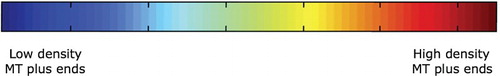
Figure 3. Vortices are obtained with kinesin-1 motors when motor activity C is low (C=1). Top row: MT and motor densities. Here, $k_{\mathrm{on}}^{\max }=10/s$, $k_{\mathrm{off}}=0.1/s$, $\Vert {\mathbf{\text{v}}}_{\mathbf{\text{b}}}\Vert =0.8\text{μ}\mathrm{m}/\mathrm{s}$, and total motor density is low ($0.05\text{μ}{\mathrm{m}}^{-2}$). (a) MT density over $(x-y)$ domain, (b) bound motor density over $(x-y)$ domain, and (c) unbound motor density over $(x-y)$ domain. Bottom row: MT orientations. (d) Orientation of MTs over $(x-y)$ domain. (e) Orientation of MTs over small portion of the $(x-y)$ domain. Vortex pattern highlighted by blue arrows.

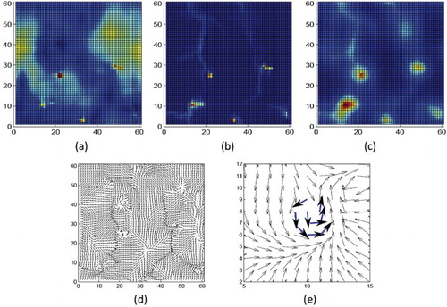
Figure 4. Plus-end focused asters are obtained with kinesin-1 motors when motor activity C is moderate (C=10). Top Row: MT and motor densities. Here, $k_{\mathrm{on}}^{\max }=10/s$, $k_{\mathrm{off}}=0.1/s$, $\Vert {\mathbf{\text{v}}}_{\mathbf{\text{b}}}\Vert =0.8\text{μ}\mathrm{m}/\mathrm{s}$, and total motor density is low ($0.05\text{μ}{\mathrm{m}}^{-2}$). (a) MT density over $(x-y)$ domain, (b) bound motor density over $(x-y)$ domain, and (c) unbound motor density over $(x-y)$ domain. Bottom row: MT orientations. (a) Orientation of MTs over $(x-y)$ domain. (b) Orientation of MTs over small portion of the $(x-y)$ domain. Aster pattern highlighted by blue arrows (arrow head represents the plus-end of a MT).

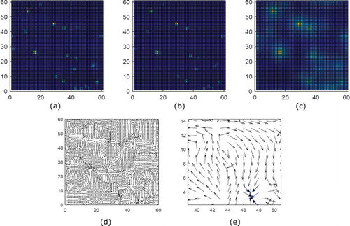
In Figure 3, we show that at high treadmilling speed, and for low motor densities, MTs form vortices when the activity of the motor is low (C is a low value). Here, we define vortex formation as a vector field that clearly shows rotation. In Figure 4, we show that plus-end asters instead of vortices form when motor activity C is increased from low to moderate. We note that motors (both bound and unbound) are primarily located at the centres of either the vortices or the asters.

These results are consistent with the results by Surrey et al. [26]. In their experiments, motors form MTs into vortices at low motor density and plus-end focused asters at higher motor densities. Further, motors were concentrated at the centres of asters and vortices, consistent with experiment [26] (results not shown here). Our experiments are slightly different, since we are increasing the motor activity parameter C and not the motor density. However, a change in C has the same alignment affect as a change in the bound motor density (since the alignment function $\kappa \left(m_{\mathrm{b}}\right)=C{m}_{\mathrm{b}}$). According to our model formulation, the numerical results suggest that vortex formation is a direct result of the crosslinking capability of motors. In particular, if motors strongly crosslink MTs, they will form aster-type patterns. Since motors are only located in the centre of either the vortices or asters, this result is rather intuitive. That is, one would expect MT plus ends to be very close together (like in an aster), if motors are crosslinking MTs there. Alternatively, if the motors are not crosslinking the MTs, the MT minus ends will not be focused (like in a vortex).

5. Conclusion

There is a trend in Mathematical Biology to avoid complicated existence and uniqueness proofs, and instead focus on numerical simulations. Our paper is a reminder that developing existence and uniqueness results is not always an academic exercise, but may lead to important insights. Here we found that the original model, as formulated in [33, 35], needed to be extended to obtain a mathematically well-defined problem. The key assumption is the local smoothing of the motor velocity ${\mathbf{\text{v}}}_{\mathrm{b}}^{\epsilon }$ in (5(6) $\frac{\mathrm{d}x\left(s\right)}{\mathrm{d}s}={\mathbf{\text{v}}}_b^{\epsilon }\left(p\right(x\left(s\right),s,\theta \left)\right).$(6) ). In the analysis, we used an index $c_{\epsilon }$ to keep track of the mollifier parameter $\epsilon >0$. The critical estimate is (20), where we estimate the divergence of ${\mathbf{\text{v}}}_{\mathbf{\text{b}}}^{\epsilon }$. In this estimate, the constant $c_{\epsilon }$ might diverge to ∞ for $\epsilon \to 0$. Hence the existence time τ must be chosen smaller for smaller values of $\epsilon >0$. After careful study of other constructions, we are convinced that the mollification (5(6) $\frac{\mathrm{d}x\left(s\right)}{\mathrm{d}s}={\mathbf{\text{v}}}_b^{\epsilon }\left(p\right(x\left(s\right),s,\theta \left)\right).$(6) ) is necessary to use such a fixed point argument. In fact, Golse et al. [5] showed that by integration of a transport equation, one gains about 1/2-order of regularity. Thus, if $p\in L^2$, then ${\mathbf{\text{v}}}_{\mathbf{\text{b}}}\in W^{1/2,2}$. However, in the first equation we need a derivative of ${\mathbf{\text{v}}}_{\mathbf{\text{b}}}$ which has regularity less than $L^2$. Whether existence can be proved without the use of a mollifier remains an open question.

Without embarking on a full existence theory, it is likely that we would not have discovered that this smoothing step is needed. Also, the smoothing of the motor velocity adds biological realism, since $m_{\mathrm{b}}$ and p describe densities and not individual motors or individual MTs, hence some average behaviour is plausible. A numerical method automatically adds some spatial averaging. Hence for $\epsilon$ small enough, the original and the modified model have the same numerical output.

Simulations of the model (with $\epsilon =0$) yield results similar to in vitro experiments [19]. In particular, simulations of MT dynamics in the presence of motors with properties similar to kinesin-1 show that MTs form vortices at low motor activity and asters at higher motor activity. The patterns determined by simulation are stable (as observed by examining numerical results only), where patterns form over a few minutes. In the experiments of [19], patterns form anywhere between 10 and 20 minutes.

Although simulation results are consistent with experimental results, there are a number of model limitations that should be considered in future work. One such limitation is that we do not take into account MT length, and just the MT ends (in the case of the simulations shown here, we only consider MT plus-ends). In general, motor proteins can attach and detach along the entire length of a MT, and so this consideration is potentially important. Further, MTs generally are very dynamic, undergoing periods of growth and shortening. These dynamics most likely play a role in overall MT organization, and so incorporation of growth dynamics is also an important future consideration.

An interesting feature of our model is that it can be extended to incorporate more than one motor type, by simply adding two more differential equations for a second type of bound and unbound motors. The authors examine this case in  [35] and find that, by using motor properties similar to properties of mitotic motors (motors that aid in mitosis), arrays of anti-parallel MTs form. This result is consistent with in vivo organization, since MTs form anti-parallel bundles (called the mitotic spindle) during cell division. This model is the first mathematical model to predict the mitotic spindle [35].

It would be interesting to extend the result to other domains. If we consider bounded domains, we need to make sure to define boundary conditions only on the inward-pointing part of the boundary. Since the characteristic velocity ${\mathbf{\text{v}}}_{\mathbf{\text{b}}}^{\epsilon }$ varies over space, it can happen that the inward and outward pointing part of a boundary form non-connected subsets of the boundary. It is unclear how to properly define boundary conditions in such a case. In addition, the transport equation would need some form of reflective boundary conditions, which are quite cumbersome to deal with. In this paper we use periodic boundary conditions. However, in the simplified model of White et al. [34], no-flux boundary conditions were implemented by using a bounce-back algorithm, where MTs bounce back inside one grid point and reorient when they have reached the boundary. This method is explained in detail in [33, 34]. The theory can be extended to $Q_{\tau }={\mathbb{R}}^n$, where we then need to use a weighted space and the appropriate solution semigroups on those spaces. We leave this idea for future work.

Disclosure statement

No potential conflict of interest was reported by the authors.

Additional information

Funding

This work was supported by National Science Foundation [DMS-1554896] and the Natural Sciences and Engineering Research Council of Canada (NSERC).

References

- I. Aranson and L. Tsimring, Pattern formation of microtubules and motors: Inelastic interaction of polar rods, Phys. Rev. 71 (2005), pp. 050901.
- I. Aranson and L. Tsimring, Theory of self-assembly of microtubule and motors, Phys. Rev. E74 (2006), pp. 031915. 1–15.
- A. Bressan, Hyperbolic Systems of Conservation Laws, Oxford University Press, Oxford, 2000.
- L.C. Evans, Partial Differential Equations, AMS Press, Rhodes Island, 1998.
- F. Golse, P.L. Lions, B. Perthame, and R. Sentis, Regularity of the moments of the solution of a transport equation, J. Funct. Anal. 76 (1988), pp. 110–125. doi: 10.1016/0022-1236(88)90051-1
- T. Hillen, P. Hinow, and Z. Wang, Mathematical analysis of a kinetic model for cell movement in tissue networks, Discr. Contin. Dyn. Syst. Ser. B 14(3) (2010), pp. 1055–1080. doi: 10.3934/dcdsb.2010.14.1055
- J. Howard, Mechanics of Motor Proteins and the Cytoskeleton, Sinauer Associates Inc., Sunderland, MA, 2001.
- D. Humphrey, C. Duggan, D. Saha, D. Smith, and J. Ka, Active fluidization of polymer networks through molecular motors, Lett. Nat. 416 (2002), pp. 413–416. doi: 10.1038/416413a
- Z. Jia, D. Karpeev, I. Aranson, and P. Bates, Simulation studies of self-organization of microtubules and molecular motors, Phys. Rev. E77 (2008), pp. 051905, 1–8.
- N. Johnson and L. Kotz, Distributions in Statistics-Continuous Univariate Distributions, 2nd ed., John Wiley and Sons, Hoboken, 1970.
- G. Karp, Cell and Molecular Biology, 1st ed., John Wiley and Sons, Inc., Hoboken, 1996.
- J. Kim, Y. Park, B. Kahng, and H. Y. Lee, Self-organized patterns in mixtures of microtubules and motor proteins, J. Kor. Phys. Soc. 42(1) (2003), pp. 162–166.
- M. Kirschner and K. Mitchison, Dynamic instability of microtubule growth, Nature 312 (1984), pp. 237–242. doi: 10.1038/312237a0
- H.Y. Lee, Macroscopic equations for pattern formation in mixtures of microtubules and molecular motors, Phys. Rev. 64 (2001), pp. 056113, 1–8.
- W. Luo, C.H. Yu, Z. Lieu, J. Allard, A. Mogilner, M. Sheetz, and A. Bershadsky, Analysis of the local organization and dynamics of cellular actin networks, J. Cell Biol. 202 (2013), pp. 1057–1073. doi: 10.1083/jcb.201210123
- C. Miller, G. Ermentrout, and L. Davidson, Rotational model for actin filament alignment by myosin, J. Theor. Biol. 300 (2012), pp. 344–359. doi: 10.1016/j.jtbi.2012.01.036
- K. Mitchison and M. Kirschner, Beyond self-assembly: From microtubules to morphogenesis, Cell 45 (1986), pp. 329–342. doi: 10.1016/0092-8674(86)90283-7
- F. Nedelec and T. Surrey, Dynamics of microtubule aster formation by motor complexes, Phys. Scale Cell 4 (2001), pp. 841–847.
- F. Nedelec, T. Surrey, A.C. Maggs, and S. Leibler, Self-organization of microtubules and motors, Nature 389 (1997), pp. 305–308. doi: 10.1038/38532
- H. Othmer, S. Dunbar, and W. Alt, Models of dispersal in biological systems, J. Math. Biol. 26 (1988), pp. 263–298. doi: 10.1007/BF00277392
- A. Pazy, Semigroups of Linear Operators and Applications to Partial Differential Equations, Springer-Verlag, New York, 1983.
- A.C. Reymann, J.L. Martiel, T. Cambier, L. Blanchoin, R. Boujemaa-Paterski, and M. Théry, Nucleation geometry governs ordered actin network structures, Nat. Mater. 9 (2010), pp. 827–832. doi: 10.1038/nmat2855
- J. Robinson, Infinite-Dimensional Dynamical Systems, 1st ed., Ordinary Differential Equations, Cambridge University Press, Cambridge, 2001.
- V. Rodionov, E. Nadezhdina, and G. Borisy, Centrosomal control of microtubule dynamics, Proc. Natl. Acad. Sci. 96 (1999), pp. 115–120. doi: 10.1073/pnas.96.1.115
- D. Smith, F. Ziebert, D. Humphrey, C. Duggan, M. Steinbeck, W. Zimmermann, and J. Ka, Molecular motor-induced instabilities and cross linkers determine biopolymer organization, Biophys. J. 93 (2007), pp. 4445–4452. doi: 10.1529/biophysj.106.095919
- T. Surrey, F. Nedelec, S. Leibler, and E. Karsenti, Physical properties determining self-organization of motors and microtubules, Science 292 (2001), pp. 1167–1171. doi: 10.1126/science.1059758
- L. Tao, A. Mogliner, G. Civelekoglu-Scholey, R. Wollman, J. Evans, H. Stahlberg, and J. Scholey, A homotetrameric kinesin-5, klp61f, bundles microtubules and antagonizes Ncd in motility assays, Curr. Biol. 16 (2006), pp. 2293–2302. doi: 10.1016/j.cub.2006.09.064
- M. Taylor, Partial Differential Equations 3, Springer-Verlag, New York, 1996.
- R. Vale, F. Malik, and D. Brown, Directional instability of microtubule transport in the presence of kinesin and dynein, two opposite polarity motor proteins, J. Cell Biol. 119 (1992), pp. 1589–1596. doi: 10.1083/jcb.119.6.1589
- R.H. Wade, On and around microtubules: an overview, Mol. Biotechnol. 43 (2009), pp. 177–191. doi: 10.1007/s12033-009-9193-5
- C.M. Waterman-Storer and E.D. Salmon, Microtubule dynamics: treadmilling comes around again, Curr. Biol. 7 (1997), pp. 369–372. doi: 10.1016/S0960-9822(06)00177-1
- C.M. Waterman-Storer and E.D. Salmon, Microtubules: strange polymers inside the cell, Bioelectro-Chem. Bioenerget. 48 (1999), pp. 285–295. doi: 10.1016/S0302-4598(99)00011-2
- D. White, Microtubule organization in the presence of motor proteins. Ph.D. thesis, University of Alberta, 2013.
- D. White, G. de Vries, and A. Dawes, Microtubule patterning in the presence of stationary motor distributions, Bull. Math. Biol. 76(8) (2014), pp. 1917–1940. doi: 10.1007/s11538-014-9991-1
- D. White, G. de Vries, J. Martin, and A. Dawes, Microtubule patterning in the presence of moving motors, J. Theor. Biol. 382 (2015), pp. 81–90. doi: 10.1016/j.jtbi.2015.06.040