Modelling the effect of immigration on drinking behaviour

ABSTRACT

A drinking model with immigration is constructed. For the model with problem drinking immigration, the model admits only one problem drinking equilibrium. For the model without problem drinking immigration, the model has two equilibria, one is problem drinking-free equilibrium and the other is problem drinking equilibrium. By employing the method of Lyapunov function, stability of all kinds of equilibria is obtained. Numerical simulations are also provided to illustrate our analytical results. Our results show that alcohol immigrants increase the difficulty of the temperance work of the region.

KEYWORDS:

• Drinking
• immigration
• equilibrium
• global stability
• Lyapunov function

AMS SUBJECT CLASSIFICATION:

• 92D25

1. Introduction

Epidemic models become a subject of concern by the bio-mathematical researchers in the modern society. In order to analyse and predict the spread of infectious disease, many epidemic models are studied in [1, 7, 8, 14, 25, 27, 34, 37]. In recent years, Huo et al.  [6] discussed the global dynamics of a novel HIV/AIDS epidemic model in which they incorporate a new compartment, that is, treatment compartment T. Huo and Zou [12] introduced a tuberculosis model with two kinds of treatment, that is, treatment at home and treatment in hospital. In addition, Zhu et al.  [38] concerned with the travelling waves of a reaction–diffusion SIRQ epidemic model with relapse.

It is well known that excessive drinking can lead to many diseases. In China, the drinking rates of male and female are 84.1% and 29.3%, respectively. Alcohol-caused rates of mortality and disability are 1.3% and 3%, respectively [13].

There are many methods to quit drinking, such as self-discipline, persuading by family and friends, drugs or physical therapy. However, up to 70% or 80% of alcohol abusers relapse after treatment [20, 26]. Thus, how to quit drinking has become a new field for researchers.

Recently, many authors began to discuss the impact of social environment, fiscal taxes, laws, regulations on smoking or drinking behaviour and the impact of drinking on a number of diseases [10, 11, 19, 24, 29, 32, 35]. Lee et al.  [16] introduced a drinking model with two control functions, and analysed the optimal control strategy of the model. In addition, Thomas and Lungu  [30] established a two-sex model and studied the impact of alcohol on AIDS. Mushayabasa and Bhunu  [21] discussed the effect of heavy alcohol consumption on the transmission dynamics of gonorrhea. Temporary abstainers could relapse by many reasons, such as body pain, intractable insomnia and so on. Cintrón-Arias et al.  [3] addressed the role of relapse on drinking dynamics. Xiang et al.  [36] studied a drinking model taking into account the compartment of permanent quitting drinker and relapse, Huo and Song  [9] studied the more realistic two-stage model for binge drinking problem, where the youths with alcohol problems were divided into those who admit to the problem and those who do not admit. They also considered the direct transfer from the class of susceptible individuals towards the class of admitting drinkers.

With the development of economic globalization, there are more and more trade exchanges and tourism activities among the countries. So, the activities of the foreign population also start to impact the economic, politics and culture. In many countries, wine as a kind of culture gradually is accepted by people. The wine is also becoming a necessity of an enhancing friendship in international trade. Custom and drinking behaviour of the different regions are mixing with each other. Due to the immigration of the foreign population, many models with immigration in different environments were studied [4, 17, 18, 39].

The people in the different areas have different living, including drinking behaviour, beliefs and so on. Immigration will bring these habits to the resettlement areas, and transmit these habits to the people around them. On the other hand, we need to persuade immigrants who have problems in drinking to stop drinking. Hence, immigrants who have problems in drinking have an impact on the drinking environment. They make the work of quitting drinking more difficult to do. So it is meaningful to study the model with immigration.

Motivated by the above, we study a quitting drinking model with immigration. Immigrants are divided into three parts, that is, immigrants who enter into the compartment of moderate drinkers, immigrants who enter into the compartment of light alcoholics and immigrants who enter into the compartment of heavy alcoholics. We mainly consider the effect of immigration on drinking behaviour.

The organization of this paper is as follows: in Section 2, the model and some basic properties of the model are derived and proved. In Section 3, the existence and stability of equilibria are proved. Some numerical simulations are also given in Section 4. The paper ends with a discussion in Section 5.

2. The model formulation

2.1. System description

From research group of treatment and rehabilitation of the U.S. National Institute on Alcohol Abuse and Alcoholism (NIAAA), in the United States, one ‘standard’ drink contains roughly 14 g of pure alcohol, which is found in: 12 ounces of regular beer, which is usually about $5\mathrm{\%}$ alcohol; 5 ounces of wine, which is typically about $12\mathrm{\%}$ alcohol; 1.5 ounces of distilled spirits, which is about $40\mathrm{\%}$ alcohol. The daily alcohol consumption for men is no more than four standard drinks, women are no more than three standard drinks. The ceiling of ‘low-risk’ alcohol consumption per week is 14 standard drinks for men, and 7 standard drinks for women [22]. If a person whose alcohol consumption is more than daily or weekly drinking ceiling, he/she most likely develop to ‘abuse alcohol’ or ‘addicted alcohol’. According to the standard of the NIAAA, similar standard can also be found in [2], the total population is divided into four compartments in this paper. The moderate drinkers (P), that is, those who drink within daily and weekly limits. Light alcoholics (L), that is, the drinkers who drink beyond daily or weekly ceiling and drink 4–5 standard drinks per day, heavy alcoholics (S), that is, the drinkers who drink more than daily and weekly limits and drink more than five standard drinks per day. Treatment compartment (Q), that is, the people who have been received treatments by taking pills or other medical interventions after alcoholism.

Modern medical research shows that drinking a little wine and beer is good for one's health. However, drinking liquor more than two cups will increase the risk of the diabetes [28]. So moderate alcohol consumption is not danger for one's health. Hence, in our model we do not consider death rate caused by drinking in $P\left(t\right)$. There are four ways for moderate drinkers to enter into compartment of light alcoholics in our model. First, moderate drinkers increase their own alcohol consumption by themselves ($\epsilon P$). Second, moderate drinkers contact with light alcoholics ($\xi PL$). Third, moderate drinkers contact with heavy alcoholics ($\alpha PS$). Fourth, moderate drinkers contact with alcoholics in treatment compartment ($\beta PQ$). We assume that at any moment time, light alcoholics leave at a rate ω, and enter into compartment of heavy alcoholics or treatment. A proportion p $(0<p<1)$ of these individuals ($p\omega L$) is assumed to be entered into treatment compartment Q and the complementary proportion $(1-p)\omega L$, move to compartment of heavy alcoholics S. The people in Q are the people who have been received treatments by taking pills or other medical interventions after alcoholism. These people may relapse drinking again or quit drinking for ever. For the simplicity, we only consider the one relapse, that is, the people in Q go back into L.

The parameter description and transfer diagram are shown in Table 1 and Figure 1, respectively.

Figure 1. Transfer diagram for the drinking model.

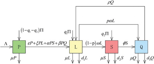
Table 1. State variables and parameters of quit drinking model.

Parameter	Description
$P\left(t\right)$	The number of moderate drinkers at time t
$L\left(t\right)$	The number of light alcoholics at time t
$S\left(t\right)$	The number of heavy alcoholics at time t
$Q\left(t\right)$	The number of the treatment of alcoholics at time t
Λ	The total recruitment rate
Π	The total number of population immigrants
$q_i,i=1,2$	The proportion of Π who enter into light alcoholics and heavy alcoholics, respectively
ρ	Treatment failure rate
ϵ	The rate which moderate drinkers increase their own alcohol consumption
ξ	The rate which moderate drinkers contact with light alcoholics
α	The rate which moderate drinkers contact with heavy alcoholics
β	The rate which moderate drinkers contact with the alcoholics being treated
φ	Treating rate of heavy alcoholics
ω	The departure rate of light alcoholics which enter into compartment of heavy alcoholics or treatment
μ	Per-person departure rate from the drinking environment
$d_i,i=1,2,3$	The drinking-related death rate
p	Treating rate of light alcoholics

From Figure 1, the following drinking model is formulated: (1) $\begin{array}{rl}\frac{\mathrm{d}P}{\mathrm{d}t}& =\mathrm{\Lambda }+(1-q_1-q_2)\mathrm{\Pi }-\epsilon P-\xi PL-\alpha PS-\beta PQ-\mu P,\\ \frac{\mathrm{d}L}{\mathrm{d}t}& =q_1\mathrm{\Pi }+\epsilon P+\xi PL+\alpha PS+\beta PQ+\rho Q-(\mu +d_1+\omega )L,\\ \frac{\mathrm{d}S}{\mathrm{d}t}& =q_2\mathrm{\Pi }+(1-p)\omega L-(\mu +d_2+\phi )S,\\ \frac{\mathrm{d}Q}{\mathrm{d}t}& =p\omega L+\phi S-(\mu +d_3+\rho )Q,\\ N& =P+L+S+Q,\end{array}$(1) where $\epsilon ,\xi ,\alpha$ and β denote the per-capita effective contact rate (transmission rate). μ denotes the per-capita departure rate from the drinking environment. ρ denotes treatment failure rate. ω denotes the departure rate of light alcoholics which enter into compartment of heavy alcoholics or treatment. φ denotes treating rate of heavy alcoholics. Λ denotes the total recruitment rate only by birth. Π represents the total number of population immigrants. Π is divided into three parts, that is, immigrants who enter into the compartment of moderate drinkers, immigrants who enter into the compartment of light alcoholics and immigrants who enter into the compartment of heavy alcoholics. $q_1$ and $q_2$ are the proportion of Π who enter into light alcoholics and heavy alcoholics, respectively. $d_i,i=1,2,3$, are the drinking-related death rate. In addition, light alcoholics are kinds of sensitive people, when they realized the dangers of alcohol, they will choose the treatment quickly; on the contrary, they are more likely to develop into heavy alcoholics or stay in the light alcoholic state. Hence, a proportion p $(0<p<1)$ denotes the treating rate of light alcoholics and the complementary proportion 1−p denote the rate of the light alcoholics develop into heavy alcoholics.

2.2. Positivity and boundedness of solutions

For system (1(1) $\begin{array}{rl}\frac{\mathrm{d}P}{\mathrm{d}t}& =\mathrm{\Lambda }+(1-q_1-q_2)\mathrm{\Pi }-\epsilon P-\xi PL-\alpha PS-\beta PQ-\mu P,\\ \frac{\mathrm{d}L}{\mathrm{d}t}& =q_1\mathrm{\Pi }+\epsilon P+\xi PL+\alpha PS+\beta PQ+\rho Q-(\mu +d_1+\omega )L,\\ \frac{\mathrm{d}S}{\mathrm{d}t}& =q_2\mathrm{\Pi }+(1-p)\omega L-(\mu +d_2+\phi )S,\\ \frac{\mathrm{d}Q}{\mathrm{d}t}& =p\omega L+\phi S-(\mu +d_3+\rho )Q,\\ N& =P+L+S+Q,\end{array}$(1) ), to ensure the solutions of the system with positive initial conditions remain positive for all t>0, it is necessary to prove that all the variables are positive. Since the solutions $\left(P\right(t)$, $L\left(t\right)$, $S\left(t\right)$, $Q\left(t\right))$ of system (1(1) $\begin{array}{rl}\frac{\mathrm{d}P}{\mathrm{d}t}& =\mathrm{\Lambda }+(1-q_1-q_2)\mathrm{\Pi }-\epsilon P-\xi PL-\alpha PS-\beta PQ-\mu P,\\ \frac{\mathrm{d}L}{\mathrm{d}t}& =q_1\mathrm{\Pi }+\epsilon P+\xi PL+\alpha PS+\beta PQ+\rho Q-(\mu +d_1+\omega )L,\\ \frac{\mathrm{d}S}{\mathrm{d}t}& =q_2\mathrm{\Pi }+(1-p)\omega L-(\mu +d_2+\phi )S,\\ \frac{\mathrm{d}Q}{\mathrm{d}t}& =p\omega L+\phi S-(\mu +d_3+\rho )Q,\\ N& =P+L+S+Q,\end{array}$(1) ) with initial data $P\left(0\right)>0,L\left(0\right)>0,S\left(0\right)>0,Q\left(0\right)>0$ are all inward on the boundaries of the feasible domain, we thus have the following lemma.

Lemma 2.1

If $P\left(0\right)>0,L\left(0\right)>0,S\left(0\right)>0,Q\left(0\right)>0,$ then the solution $P\left(t\right),$ $L\left(t\right),$ $S\left(t\right),$ $Q\left(t\right)$ of system (1(1) $\begin{array}{rl}\frac{\mathrm{d}P}{\mathrm{d}t}& =\mathrm{\Lambda }+(1-q_1-q_2)\mathrm{\Pi }-\epsilon P-\xi PL-\alpha PS-\beta PQ-\mu P,\\ \frac{\mathrm{d}L}{\mathrm{d}t}& =q_1\mathrm{\Pi }+\epsilon P+\xi PL+\alpha PS+\beta PQ+\rho Q-(\mu +d_1+\omega )L,\\ \frac{\mathrm{d}S}{\mathrm{d}t}& =q_2\mathrm{\Pi }+(1-p)\omega L-(\mu +d_2+\phi )S,\\ \frac{\mathrm{d}Q}{\mathrm{d}t}& =p\omega L+\phi S-(\mu +d_3+\rho )Q,\\ N& =P+L+S+Q,\end{array}$(1) ) is positive for all t>0.

Lemma 2.2

All feasible solutions of the system (1(1) $\begin{array}{rl}\frac{\mathrm{d}P}{\mathrm{d}t}& =\mathrm{\Lambda }+(1-q_1-q_2)\mathrm{\Pi }-\epsilon P-\xi PL-\alpha PS-\beta PQ-\mu P,\\ \frac{\mathrm{d}L}{\mathrm{d}t}& =q_1\mathrm{\Pi }+\epsilon P+\xi PL+\alpha PS+\beta PQ+\rho Q-(\mu +d_1+\omega )L,\\ \frac{\mathrm{d}S}{\mathrm{d}t}& =q_2\mathrm{\Pi }+(1-p)\omega L-(\mu +d_2+\phi )S,\\ \frac{\mathrm{d}Q}{\mathrm{d}t}& =p\omega L+\phi S-(\mu +d_3+\rho )Q,\\ N& =P+L+S+Q,\end{array}$(1) ) are bounded and enter the region $\mathrm{\Omega }=\left\{(P,L,S,Q)\in R_{+}^4:P+L+S+Q\le \frac{\mathrm{\Lambda }+\mathrm{\Pi }}{\mu }\right\}.$

Proof.

Let $(P,L,S,Q)\in R_{+}^4$ be any solution with positive initial condition, adding the first four equations of Equation (1(1) $\begin{array}{rl}\frac{\mathrm{d}P}{\mathrm{d}t}& =\mathrm{\Lambda }+(1-q_1-q_2)\mathrm{\Pi }-\epsilon P-\xi PL-\alpha PS-\beta PQ-\mu P,\\ \frac{\mathrm{d}L}{\mathrm{d}t}& =q_1\mathrm{\Pi }+\epsilon P+\xi PL+\alpha PS+\beta PQ+\rho Q-(\mu +d_1+\omega )L,\\ \frac{\mathrm{d}S}{\mathrm{d}t}& =q_2\mathrm{\Pi }+(1-p)\omega L-(\mu +d_2+\phi )S,\\ \frac{\mathrm{d}Q}{\mathrm{d}t}& =p\omega L+\phi S-(\mu +d_3+\rho )Q,\\ N& =P+L+S+Q,\end{array}$(1) ), we have $\begin{array}{rl}\frac{\mathrm{d}}{\mathrm{d}t}(P+L+S+Q)& =\mathrm{\Lambda }+\mathrm{\Pi }-\mu P-\mu L-\mu S-\mu Q-d_{1}L-d_{2}S-d_{3}Q\\ & =\mathrm{\Lambda }+\mathrm{\Pi }-\mu (P+L+S+Q)-(d_{1}L+d_{2}S+d_{3}Q)\\ & \le \mathrm{\Lambda }+\mathrm{\Pi }-\mu (P+L+S+Q)\\ & =\mathrm{\Lambda }+\mathrm{\Pi }-\mu N\left(t\right).\end{array}$ It follows that $0\le N\left(t\right)\le \frac{\mathrm{\Lambda }+\mathrm{\Pi }}{\mu }+\left(N\left(0\right)-\frac{\mathrm{\Lambda }+\mathrm{\Pi }}{\mu }\right){\mathrm{e}}^{-\mu t},$ where $N\left(0\right)$ represents initial value of the total population. Thus $0\le N\left(t\right)\le \frac{\mathrm{\Lambda }+\mathrm{\Pi }}{\mu }$, as $t\to \mathrm{\infty }$. Therefore all feasible solutions of system (1(1) $\begin{array}{rl}\frac{\mathrm{d}P}{\mathrm{d}t}& =\mathrm{\Lambda }+(1-q_1-q_2)\mathrm{\Pi }-\epsilon P-\xi PL-\alpha PS-\beta PQ-\mu P,\\ \frac{\mathrm{d}L}{\mathrm{d}t}& =q_1\mathrm{\Pi }+\epsilon P+\xi PL+\alpha PS+\beta PQ+\rho Q-(\mu +d_1+\omega )L,\\ \frac{\mathrm{d}S}{\mathrm{d}t}& =q_2\mathrm{\Pi }+(1-p)\omega L-(\mu +d_2+\phi )S,\\ \frac{\mathrm{d}Q}{\mathrm{d}t}& =p\omega L+\phi S-(\mu +d_3+\rho )Q,\\ N& =P+L+S+Q,\end{array}$(1) ) enter the region $\mathrm{\Omega }=\left\{(P,L,S,Q)\in R_{+}^4:P+L+S+Q\le \frac{\mathrm{\Lambda }+\mathrm{\Pi }}{\mu }\right\}.$ The vector field along the boundary of Ω points inward, so that Ω is forward invariant. Hence, Ω is positively invariant and it is sufficient to consider solutions of system (1(1) $\begin{array}{rl}\frac{\mathrm{d}P}{\mathrm{d}t}& =\mathrm{\Lambda }+(1-q_1-q_2)\mathrm{\Pi }-\epsilon P-\xi PL-\alpha PS-\beta PQ-\mu P,\\ \frac{\mathrm{d}L}{\mathrm{d}t}& =q_1\mathrm{\Pi }+\epsilon P+\xi PL+\alpha PS+\beta PQ+\rho Q-(\mu +d_1+\omega )L,\\ \frac{\mathrm{d}S}{\mathrm{d}t}& =q_2\mathrm{\Pi }+(1-p)\omega L-(\mu +d_2+\phi )S,\\ \frac{\mathrm{d}Q}{\mathrm{d}t}& =p\omega L+\phi S-(\mu +d_3+\rho )Q,\\ N& =P+L+S+Q,\end{array}$(1) ) in Ω. Existence, uniqueness and continuation results for system (1(1) $\begin{array}{rl}\frac{\mathrm{d}P}{\mathrm{d}t}& =\mathrm{\Lambda }+(1-q_1-q_2)\mathrm{\Pi }-\epsilon P-\xi PL-\alpha PS-\beta PQ-\mu P,\\ \frac{\mathrm{d}L}{\mathrm{d}t}& =q_1\mathrm{\Pi }+\epsilon P+\xi PL+\alpha PS+\beta PQ+\rho Q-(\mu +d_1+\omega )L,\\ \frac{\mathrm{d}S}{\mathrm{d}t}& =q_2\mathrm{\Pi }+(1-p)\omega L-(\mu +d_2+\phi )S,\\ \frac{\mathrm{d}Q}{\mathrm{d}t}& =p\omega L+\phi S-(\mu +d_3+\rho )Q,\\ N& =P+L+S+Q,\end{array}$(1) ) hold in this region. It can be shown that $N\left(t\right)$ is bounded and all the solutions which start in Ω approach, enter or stay in Ω.

3. Analysis of the model

In this section, we will analyse the qualitative behaviour of system (1(1) $\begin{array}{rl}\frac{\mathrm{d}P}{\mathrm{d}t}& =\mathrm{\Lambda }+(1-q_1-q_2)\mathrm{\Pi }-\epsilon P-\xi PL-\alpha PS-\beta PQ-\mu P,\\ \frac{\mathrm{d}L}{\mathrm{d}t}& =q_1\mathrm{\Pi }+\epsilon P+\xi PL+\alpha PS+\beta PQ+\rho Q-(\mu +d_1+\omega )L,\\ \frac{\mathrm{d}S}{\mathrm{d}t}& =q_2\mathrm{\Pi }+(1-p)\omega L-(\mu +d_2+\phi )S,\\ \frac{\mathrm{d}Q}{\mathrm{d}t}& =p\omega L+\phi S-(\mu +d_3+\rho )Q,\\ N& =P+L+S+Q,\end{array}$(1) ).

3.1. Existence of equilibria and the basic reproduction number

The equilibrium of system (1(1) $\begin{array}{rl}\frac{\mathrm{d}P}{\mathrm{d}t}& =\mathrm{\Lambda }+(1-q_1-q_2)\mathrm{\Pi }-\epsilon P-\xi PL-\alpha PS-\beta PQ-\mu P,\\ \frac{\mathrm{d}L}{\mathrm{d}t}& =q_1\mathrm{\Pi }+\epsilon P+\xi PL+\alpha PS+\beta PQ+\rho Q-(\mu +d_1+\omega )L,\\ \frac{\mathrm{d}S}{\mathrm{d}t}& =q_2\mathrm{\Pi }+(1-p)\omega L-(\mu +d_2+\phi )S,\\ \frac{\mathrm{d}Q}{\mathrm{d}t}& =p\omega L+\phi S-(\mu +d_3+\rho )Q,\\ N& =P+L+S+Q,\end{array}$(1) ) satisfies the following system of algebraic equation (2) $\begin{array}{rl}\mathrm{\Lambda }+(1-q_1-q_2)\mathrm{\Pi }-\epsilon P-\xi PL-\alpha PS-\beta PQ-\mu P& =0,\\ q_1\mathrm{\Pi }+\epsilon P+\xi PL+\alpha PS+\beta PQ+\rho Q-(\mu +d_1+\omega )L& =0,\\ q_2\mathrm{\Pi }+(1-p)\omega L-(\mu +d_2+\phi )S& =0,\\ p\omega L+\phi S-(\mu +d_3+\rho )Q& =0.\end{array}$(2) Let $\begin{array}{rl}a& =\mu +d_1+\omega ,\\ b& =\mu +d_2+\phi ,\\ c& =\mu +d_3+\rho ,\\ d& =p(\mu +d_2)+\phi ,\\ e& =\epsilon +\mu .\end{array}$ From the first and last two equations in Equation (2(2) $\begin{array}{rl}\mathrm{\Lambda }+(1-q_1-q_2)\mathrm{\Pi }-\epsilon P-\xi PL-\alpha PS-\beta PQ-\mu P& =0,\\ q_1\mathrm{\Pi }+\epsilon P+\xi PL+\alpha PS+\beta PQ+\rho Q-(\mu +d_1+\omega )L& =0,\\ q_2\mathrm{\Pi }+(1-p)\omega L-(\mu +d_2+\phi )S& =0,\\ p\omega L+\phi S-(\mu +d_3+\rho )Q& =0.\end{array}$(2) ), we obtain (3) $\begin{array}{rl}P& =\frac{\mathrm{\Lambda }+(1-q_1-q_2)\mathrm{\Pi }}{\xi L+\alpha [\frac{q_2\mathrm{\Pi }}{b}+\frac{(1-p)\omega }{b}L]+\beta [\frac{\mathrm{d}\omega }{bc}L+\frac{q_2\mathrm{\Pi }\phi }{bc}]+e},\\ S& =\frac{q_2\mathrm{\Pi }}{b}+\frac{(1-p)\omega }{b}L,\\ Q& =\frac{d\omega }{bc}L+\frac{q_2\mathrm{\Pi }\phi }{bc}.\end{array}$(3) Substituting Equation (3(3) $\begin{array}{rl}P& =\frac{\mathrm{\Lambda }+(1-q_1-q_2)\mathrm{\Pi }}{\xi L+\alpha [\frac{q_2\mathrm{\Pi }}{b}+\frac{(1-p)\omega }{b}L]+\beta [\frac{\mathrm{d}\omega }{bc}L+\frac{q_2\mathrm{\Pi }\phi }{bc}]+e},\\ S& =\frac{q_2\mathrm{\Pi }}{b}+\frac{(1-p)\omega }{b}L,\\ Q& =\frac{d\omega }{bc}L+\frac{q_2\mathrm{\Pi }\phi }{bc}.\end{array}$(3) ) into the second equation in Equation (2(2) $\begin{array}{rl}\mathrm{\Lambda }+(1-q_1-q_2)\mathrm{\Pi }-\epsilon P-\xi PL-\alpha PS-\beta PQ-\mu P& =0,\\ q_1\mathrm{\Pi }+\epsilon P+\xi PL+\alpha PS+\beta PQ+\rho Q-(\mu +d_1+\omega )L& =0,\\ q_2\mathrm{\Pi }+(1-p)\omega L-(\mu +d_2+\phi )S& =0,\\ p\omega L+\phi S-(\mu +d_3+\rho )Q& =0.\end{array}$(2) ), we have $\begin{array}{rl}& q_1\mathrm{\Pi }+\epsilon \left[\frac{\mathrm{\Lambda }+(1-q_1-q_2)\mathrm{\Pi }}{\xi L+\alpha [\frac{q_2\mathrm{\Pi }}{b}+\frac{(1-p)\omega }{b}L]+\beta [\frac{\mathrm{d}\omega }{bc}L+\frac{q_2\mathrm{\Pi }\phi }{bc}]+e}\right]\\ & +\xi \left[\frac{\mathrm{\Lambda }+(1-q_1-q_2)\mathrm{\Pi }}{\xi L+\alpha [\frac{q_2\mathrm{\Pi }}{b}+\frac{(1-p)\omega }{b}L]+\beta [\frac{\mathrm{d}\omega }{bc}L+\frac{q_2\mathrm{\Pi }\phi }{bc}]+e}\right]L\\ & +\alpha \left[\frac{\mathrm{\Lambda }+(1-q_1-q_2)\mathrm{\Pi }}{\xi L+\alpha [\frac{q_2\mathrm{\Pi }}{b}+\frac{(1-p)\omega }{b}L]+\beta [\frac{\mathrm{d}\omega }{bc}L+\frac{q_2\mathrm{\Pi }\phi }{bc}]+e}\right]\left[\frac{q_2\mathrm{\Pi }}{b}+\frac{(1-p)\omega }{b}L\right]\\ & +\beta \left[\frac{\mathrm{\Lambda }+(1-q_1-q_2)\mathrm{\Pi }}{\xi L+\alpha [\frac{q_2\mathrm{\Pi }}{b}+\frac{(1-p)\omega }{b}L]+\beta [\frac{\mathrm{d}\omega }{bc}L+\frac{q_2\mathrm{\Pi }\phi }{bc}]+e}\right]\left(\frac{\mathrm{d}\omega }{bc}L+\frac{q_2\mathrm{\Pi }\phi }{bc}\right)\\ & +\rho \left(\frac{\mathrm{d}\omega }{bc}L+\frac{q_2\mathrm{\Pi }\phi }{bc}\right)-aL=0.\end{array}$ Then, we get a quadratic equation for L $f\left(L\right)=f_1{L}^2+f_{2}L+f_3=0,$ where $\begin{array}{rl}{f}_1& =\left(-a+\rho \frac{\mathrm{d}\omega }{bc}\right)\xi +\left(-a+\rho \frac{\mathrm{d}\omega }{bc}\right)\alpha \frac{(1-p)\omega }{b}+\left(-a+\rho \frac{\mathrm{d}\omega }{bc}\right)\beta \frac{\mathrm{d}\omega }{bc},\\ f_2& =q_1\mathrm{\Pi }\xi +\frac{q_1\mathrm{\Pi }\alpha (1-p)\omega }{b}+\frac{q_1\mathrm{\Pi }\beta \mathrm{d}\omega }{bc}+\xi [\mathrm{\Lambda }+(1-q_1-q_2\left)\mathrm{\Pi }\right]+\frac{\alpha \mathrm{\Lambda }(1-p)\omega }{b}\\ & +\alpha (1-q_1-q_2)\mathrm{\Pi }\frac{(1-p)\omega }{b}+\beta \mathrm{\Lambda }\frac{\mathrm{d}\omega }{bc}+\beta (1-q_1-q_2)\mathrm{\Pi }\frac{\mathrm{d}\omega }{bc}\\ & +\rho \frac{\mathrm{d}\omega }{bc}\alpha \frac{q_2\mathrm{\Pi }}{b}+\rho \frac{\mathrm{d}\omega }{bc}\beta \frac{\phi q_2\mathrm{\Pi }}{bc}+\rho \frac{\mathrm{d}\omega }{bc}e+\rho \frac{\phi q_2\mathrm{\Pi }}{bc}\xi +\rho \frac{\phi q_2\mathrm{\Pi }}{bc}\alpha \frac{(1-p)\omega }{b}\\ & +\rho \frac{\phi q_2\mathrm{\Pi }}{bc}\beta \frac{\mathrm{d}\omega }{bc}-a\alpha \frac{q_2\mathrm{\Pi }}{b}-a\beta \frac{\phi q_2\mathrm{\Pi }}{bc}-ae,\\ f_3& =\frac{q_1\mathrm{\Pi }\alpha q_2\mathrm{\Pi }}{b}+\frac{q_1\mathrm{\Pi }\beta \phi q_2\mathrm{\Pi }}{bc}+q_1\mathrm{\Pi }e+\epsilon \left[\mathrm{\Lambda }+(1-q_1-q_2)\mathrm{\Pi }\right]+\frac{\alpha \mathrm{\Lambda }{q}_2\mathrm{\Pi }}{b}\\ & +\alpha (1-q_1-q_2)\mathrm{\Pi }\frac{q_2\mathrm{\Pi }}{b}+\frac{\beta \mathrm{\Lambda }\phi q_2\mathrm{\Pi }}{bc}+\beta (1-q_1-q_2)\mathrm{\Pi }\frac{\phi q_2\mathrm{\Pi }}{bc}\\ & +\rho \frac{\phi q_2\mathrm{\Pi }}{bc}\alpha \frac{q_2\mathrm{\Pi }}{b}+\rho \frac{\phi q_2\mathrm{\Pi }}{bc}\beta \frac{\phi q_2\mathrm{\Pi }}{bc}+\rho \frac{\phi q_2\mathrm{\Pi }}{bc}e>0.\end{array}$ Note that $-a+\rho \frac{\mathrm{d}\omega }{bc}=\frac{\rho (p\mu \omega +p{d}_2\omega +\phi \omega )-(\mu +d_1+\omega )(\mu +d_2+\phi )(\mu +d_3+\rho )}{(\mu +d_2+\phi )(\mu +d_3+\rho )}<0,$ then we get $f_1<0$. The quadratic equation $f\left(L\right)=0$ always has a positive solution $L^{\ast }=\frac{f_2+\sqrt{f_2^2-4f_1{f}_3}}{-2f_1}>0$ in Ω. Substituting this value into Equation (2(2) $\begin{array}{rl}\mathrm{\Lambda }+(1-q_1-q_2)\mathrm{\Pi }-\epsilon P-\xi PL-\alpha PS-\beta PQ-\mu P& =0,\\ q_1\mathrm{\Pi }+\epsilon P+\xi PL+\alpha PS+\beta PQ+\rho Q-(\mu +d_1+\omega )L& =0,\\ q_2\mathrm{\Pi }+(1-p)\omega L-(\mu +d_2+\phi )S& =0,\\ p\omega L+\phi S-(\mu +d_3+\rho )Q& =0.\end{array}$(2) ), we get a problem drinking equilibrium $E^{\ast }(P^{\ast },L^{\ast },S^{\ast },Q^{\ast })$ in Ω, with $P^{\ast }>0,L^{\ast }>0,S^{\ast }>0,Q^{\ast }>0$.

When $q_1=q_2=0$, the model (1(1) $\begin{array}{rl}\frac{\mathrm{d}P}{\mathrm{d}t}& =\mathrm{\Lambda }+(1-q_1-q_2)\mathrm{\Pi }-\epsilon P-\xi PL-\alpha PS-\beta PQ-\mu P,\\ \frac{\mathrm{d}L}{\mathrm{d}t}& =q_1\mathrm{\Pi }+\epsilon P+\xi PL+\alpha PS+\beta PQ+\rho Q-(\mu +d_1+\omega )L,\\ \frac{\mathrm{d}S}{\mathrm{d}t}& =q_2\mathrm{\Pi }+(1-p)\omega L-(\mu +d_2+\phi )S,\\ \frac{\mathrm{d}Q}{\mathrm{d}t}& =p\omega L+\phi S-(\mu +d_3+\rho )Q,\\ N& =P+L+S+Q,\end{array}$(1) ) has no alcohol abuse immigrants. System (1(1) $\begin{array}{rl}\frac{\mathrm{d}P}{\mathrm{d}t}& =\mathrm{\Lambda }+(1-q_1-q_2)\mathrm{\Pi }-\epsilon P-\xi PL-\alpha PS-\beta PQ-\mu P,\\ \frac{\mathrm{d}L}{\mathrm{d}t}& =q_1\mathrm{\Pi }+\epsilon P+\xi PL+\alpha PS+\beta PQ+\rho Q-(\mu +d_1+\omega )L,\\ \frac{\mathrm{d}S}{\mathrm{d}t}& =q_2\mathrm{\Pi }+(1-p)\omega L-(\mu +d_2+\phi )S,\\ \frac{\mathrm{d}Q}{\mathrm{d}t}& =p\omega L+\phi S-(\mu +d_3+\rho )Q,\\ N& =P+L+S+Q,\end{array}$(1) ) becomes (4) $\begin{array}{rl}\frac{\mathrm{d}P}{\mathrm{d}t}& =\mathrm{\Lambda }+\mathrm{\Pi }-\epsilon P-\xi PL-\alpha PS-\beta PQ-\mu P,\\ \frac{\mathrm{d}L}{\mathrm{d}t}& =\epsilon P+\xi PL+\alpha PS+\beta PQ+\rho Q-(\mu +d_1+\omega )L,\\ \frac{\mathrm{d}S}{\mathrm{d}t}& =(1-p)\omega L-(\mu +d_2+\phi )S,\\ \frac{\mathrm{d}Q}{\mathrm{d}t}& =p\omega L+\phi S-(\mu +d_3+\rho )Q.\end{array}$(4) Let L=S=Q=0 in Equation (4(4) $\begin{array}{rl}\frac{\mathrm{d}P}{\mathrm{d}t}& =\mathrm{\Lambda }+\mathrm{\Pi }-\epsilon P-\xi PL-\alpha PS-\beta PQ-\mu P,\\ \frac{\mathrm{d}L}{\mathrm{d}t}& =\epsilon P+\xi PL+\alpha PS+\beta PQ+\rho Q-(\mu +d_1+\omega )L,\\ \frac{\mathrm{d}S}{\mathrm{d}t}& =(1-p)\omega L-(\mu +d_2+\phi )S,\\ \frac{\mathrm{d}Q}{\mathrm{d}t}& =p\omega L+\phi S-(\mu +d_3+\rho )Q.\end{array}$(4) ), we can obtain problem drinking-free equilibrium $E_0=\left(\mathrm{\Lambda }+\mathrm{\Pi }\right)/\mu ,0,0,0$ if $\epsilon =0$. In the following, the basic reproduction number of system (4(4) $\begin{array}{rl}\frac{\mathrm{d}P}{\mathrm{d}t}& =\mathrm{\Lambda }+\mathrm{\Pi }-\epsilon P-\xi PL-\alpha PS-\beta PQ-\mu P,\\ \frac{\mathrm{d}L}{\mathrm{d}t}& =\epsilon P+\xi PL+\alpha PS+\beta PQ+\rho Q-(\mu +d_1+\omega )L,\\ \frac{\mathrm{d}S}{\mathrm{d}t}& =(1-p)\omega L-(\mu +d_2+\phi )S,\\ \frac{\mathrm{d}Q}{\mathrm{d}t}& =p\omega L+\phi S-(\mu +d_3+\rho )Q.\end{array}$(4) ) when $\epsilon =0$ will be obtained by the next generation matrix method formulated in [31].

Let $\epsilon =0$ and $x=(L,S,Q,P{)}^{\mathrm{T}}$, then system (4(4) $\begin{array}{rl}\frac{\mathrm{d}P}{\mathrm{d}t}& =\mathrm{\Lambda }+\mathrm{\Pi }-\epsilon P-\xi PL-\alpha PS-\beta PQ-\mu P,\\ \frac{\mathrm{d}L}{\mathrm{d}t}& =\epsilon P+\xi PL+\alpha PS+\beta PQ+\rho Q-(\mu +d_1+\omega )L,\\ \frac{\mathrm{d}S}{\mathrm{d}t}& =(1-p)\omega L-(\mu +d_2+\phi )S,\\ \frac{\mathrm{d}Q}{\mathrm{d}t}& =p\omega L+\phi S-(\mu +d_3+\rho )Q.\end{array}$(4) ) can be written as $\frac{\mathrm{d}x}{\mathrm{d}t}=\mathcal{F}\left(x\right)-\mathcal{V}\left(x\right),$

where $\mathcal{F}\left(x\right)=\left(\begin{array}{c}\xi PL+\alpha PS+\beta PQ\\ 0\\ 0\\ 0\end{array}\right)$ and $\mathcal{V}\left(x\right)=\left(\begin{array}{c}(\mu +d_1+\omega )L-\rho Q\\ (\mu +d_2+\phi )S-(1-p)\omega L\\ (\mu +d_3+\rho )Q-p\omega L-\phi S\\ \xi PL+\alpha PS+\beta PQ+\mu P-\mathrm{\Lambda }-\mathrm{\Pi }\end{array}\right).$ The Jacobian matrices of $\mathcal{F}\left(x\right)$ and $\mathcal{V}\left(x\right)$ at the problem drinking-free equilibrium $E_0$ are, respectively, $D\mathcal{F}\left(E_0\right)=\left(\begin{array}{cc}{F}_{3\times 3}& 0\\ 0& 0\end{array}\right),D\mathcal{V}\left(E_0\right)=\left(\begin{array}{cc}{V}_{3\times 3}& 0\\ \frac{\xi (\mathrm{\Lambda }+\mathrm{\Pi })}{\mu }\frac{\alpha (\mathrm{\Lambda }+\mathrm{\Pi })}{\mu }\frac{\beta (\mathrm{\Lambda }+\mathrm{\Pi })}{\mu }& \mu \end{array}\right),$ where $\begin{array}{rl}F& =\left(\begin{array}{ccc}\frac{\xi (\mathrm{\Lambda }+\mathrm{\Pi })}{\mu }& \frac{\alpha (\mathrm{\Lambda }+\mathrm{\Pi })}{\mu }& \frac{\beta (\mathrm{\Lambda }+\mathrm{\Pi })}{\mu }\\ 0& 0& 0\\ 0& 0& 0\end{array}\right),\\ V& =\left(\begin{array}{ccc}\mu +d_1+\omega & 0& -\rho \\ -(1-p)\omega & \mu +d_2+\phi & 0\\ -p\omega & -\phi & \mu +d_3+\rho \end{array}\right).\end{array}$ The basic reproduction number, denoted by $R_0$ is thus given by $R_0=\rho \left(F{V}^{-1}\right)=R_1+R_2+R_3,$ where $\begin{array}{rl}{R}_1& =\frac{\xi (\mathrm{\Lambda }+\mathrm{\Pi })}{\mu }\left[\frac{1}{\mu +d_1+\omega }+\frac{\left[p\omega \right(\mu +d_2+\phi )+(1-p\left)\omega \phi \right]\rho }{\begin{array}{l}(\mu +d_1+\omega )\left[\right(\mu +d_1+\omega \left)\right(\mu +d_2+\phi )\\ \times (\mu +d_3+\rho )-\omega \phi \rho -p\omega \rho (\mu +d_2)]\end{array}}\right],\\ R_2& =\frac{\alpha (\mathrm{\Lambda }+\mathrm{\Pi })}{\mu }\\ & \times \left[\frac{(1-p)\omega }{(\mu +d_1+\omega )(\mu +d_2+\phi )}+\frac{\left[p\omega \right(\mu +d_2+\phi )+(1-p\left)\omega \phi \right](1-p)\omega \rho }{\begin{array}{l}(\mu +d_1+\omega )\left[\right(\mu +d_1+\omega \left)\right(\mu +d_2+\phi )\\ \times (\mu +d_3+\rho )-\omega \phi \rho -p\omega \rho (\mu +d_2)]\end{array}}\right],\\ R_3& =\frac{\beta (\mathrm{\Lambda }+\mathrm{\Pi })}{\mu }\cdot \frac{p\omega (\mu +d_2+\phi )+(1-p)\omega \phi }{(\mu +d_1+\omega )(\mu +d_2+\phi )(\mu +d_3+\rho )-\omega \phi \rho -p\omega \rho (\mu +d_2)}.\end{array}$

If $q_1=q_2=\epsilon =0$, system (4(4) $\begin{array}{rl}\frac{\mathrm{d}P}{\mathrm{d}t}& =\mathrm{\Lambda }+\mathrm{\Pi }-\epsilon P-\xi PL-\alpha PS-\beta PQ-\mu P,\\ \frac{\mathrm{d}L}{\mathrm{d}t}& =\epsilon P+\xi PL+\alpha PS+\beta PQ+\rho Q-(\mu +d_1+\omega )L,\\ \frac{\mathrm{d}S}{\mathrm{d}t}& =(1-p)\omega L-(\mu +d_2+\phi )S,\\ \frac{\mathrm{d}Q}{\mathrm{d}t}& =p\omega L+\phi S-(\mu +d_3+\rho )Q.\end{array}$(4) ) has a unique problem drinking equilibrium $E^{\ast \ast }$. Thus, we have the following theorem.

Theorem 3.1

If $q_1^2+q_2^2\ne 0,$ the quit drinking model (1(1) $\begin{array}{rl}\frac{\mathrm{d}P}{\mathrm{d}t}& =\mathrm{\Lambda }+(1-q_1-q_2)\mathrm{\Pi }-\epsilon P-\xi PL-\alpha PS-\beta PQ-\mu P,\\ \frac{\mathrm{d}L}{\mathrm{d}t}& =q_1\mathrm{\Pi }+\epsilon P+\xi PL+\alpha PS+\beta PQ+\rho Q-(\mu +d_1+\omega )L,\\ \frac{\mathrm{d}S}{\mathrm{d}t}& =q_2\mathrm{\Pi }+(1-p)\omega L-(\mu +d_2+\phi )S,\\ \frac{\mathrm{d}Q}{\mathrm{d}t}& =p\omega L+\phi S-(\mu +d_3+\rho )Q,\\ N& =P+L+S+Q,\end{array}$(1) ) has a unique problem drinking equilibrium $E^{\ast }(P^{\ast },L^{\ast },S^{\ast },Q^{\ast })$. If $q_1=q_2=\epsilon =0,$ the drinking model (4(4) $\begin{array}{rl}\frac{\mathrm{d}P}{\mathrm{d}t}& =\mathrm{\Lambda }+\mathrm{\Pi }-\epsilon P-\xi PL-\alpha PS-\beta PQ-\mu P,\\ \frac{\mathrm{d}L}{\mathrm{d}t}& =\epsilon P+\xi PL+\alpha PS+\beta PQ+\rho Q-(\mu +d_1+\omega )L,\\ \frac{\mathrm{d}S}{\mathrm{d}t}& =(1-p)\omega L-(\mu +d_2+\phi )S,\\ \frac{\mathrm{d}Q}{\mathrm{d}t}& =p\omega L+\phi S-(\mu +d_3+\rho )Q.\end{array}$(4) ) has a problem drinking-free equilibrium $E_0=((\mathrm{\Lambda }+\mathrm{\Pi })/\mu ,0,0,0)$ and exists a problem drinking equilibrium $E^{\ast \ast },$ where $E^{\ast \ast }$ is a special form of $E^{\ast }$ when $q_1=q_2=\epsilon =0$.

Following Theorem 2 of [31], we also have the following result on the local stability of $E_0$ of Equation (4(4) $\begin{array}{rl}\frac{\mathrm{d}P}{\mathrm{d}t}& =\mathrm{\Lambda }+\mathrm{\Pi }-\epsilon P-\xi PL-\alpha PS-\beta PQ-\mu P,\\ \frac{\mathrm{d}L}{\mathrm{d}t}& =\epsilon P+\xi PL+\alpha PS+\beta PQ+\rho Q-(\mu +d_1+\omega )L,\\ \frac{\mathrm{d}S}{\mathrm{d}t}& =(1-p)\omega L-(\mu +d_2+\phi )S,\\ \frac{\mathrm{d}Q}{\mathrm{d}t}& =p\omega L+\phi S-(\mu +d_3+\rho )Q.\end{array}$(4) ).

Theorem 3.2

If $q_1=q_2=\epsilon =0$ and $R_0<1,$ the problem drinking-free equilibrium $E_0$ of Equation (4(4) $\begin{array}{rl}\frac{\mathrm{d}P}{\mathrm{d}t}& =\mathrm{\Lambda }+\mathrm{\Pi }-\epsilon P-\xi PL-\alpha PS-\beta PQ-\mu P,\\ \frac{\mathrm{d}L}{\mathrm{d}t}& =\epsilon P+\xi PL+\alpha PS+\beta PQ+\rho Q-(\mu +d_1+\omega )L,\\ \frac{\mathrm{d}S}{\mathrm{d}t}& =(1-p)\omega L-(\mu +d_2+\phi )S,\\ \frac{\mathrm{d}Q}{\mathrm{d}t}& =p\omega L+\phi S-(\mu +d_3+\rho )Q.\end{array}$(4) ) is local asymptotically stable.

3.2. Stability of the model

Now, we discuss the global stability of equilibria of our model.

3.2.1. Stability of the equilibria

Theorem 3.3

If $q_1=q_2=\epsilon =0$ and $max\{\xi (\mathrm{\Lambda }+\mathrm{\Pi })/\mu ,\alpha (\mathrm{\Lambda }+\mathrm{\Pi })/\mu ,\beta (\mathrm{\Lambda }+\mathrm{\Pi })/\mu \}<min\{\mu +d_i,i=1,2,3\},$ the problem drinking-free equilibrium $E_0$ of Equation (4(4) $\begin{array}{rl}\frac{\mathrm{d}P}{\mathrm{d}t}& =\mathrm{\Lambda }+\mathrm{\Pi }-\epsilon P-\xi PL-\alpha PS-\beta PQ-\mu P,\\ \frac{\mathrm{d}L}{\mathrm{d}t}& =\epsilon P+\xi PL+\alpha PS+\beta PQ+\rho Q-(\mu +d_1+\omega )L,\\ \frac{\mathrm{d}S}{\mathrm{d}t}& =(1-p)\omega L-(\mu +d_2+\phi )S,\\ \frac{\mathrm{d}Q}{\mathrm{d}t}& =p\omega L+\phi S-(\mu +d_3+\rho )Q.\end{array}$(4) ) is globally asymptotically stable.

Proof.

We introduce the following Lyapunov function: $V=P_0\left(\frac{P}{P_0}-\ln \frac{P}{P_0}\right)+L+S+Q.$ The derivative of V is given by $\begin{array}{rl}{V}^{\mathrm{\prime }}& =P^{\mathrm{\prime }}-\frac{P_0}{P}{P}^{\mathrm{\prime }}+L^{\mathrm{\prime }}+S^{\mathrm{\prime }}+Q^{\mathrm{\prime }}\\ & =2(\mathrm{\Lambda }+\mathrm{\Pi })-\mu P-\frac{(\mathrm{\Lambda }+\mathrm{\Pi }{)}^2}{\mu P}+\frac{\xi (\mathrm{\Lambda }+\mathrm{\Pi })}{\mu }L+\frac{\alpha (\mathrm{\Lambda }+\mathrm{\Pi })}{\mu }S+\frac{\beta (\mathrm{\Lambda }+\mathrm{\Pi })}{\mu }Q\\ & -(\mu +d_1)L-(\mu +d_2)S-(\mu +d_3)Q\\ & =\left(2-\frac{\mu P}{\mathrm{\Lambda }+\mathrm{\Pi }}-\frac{\mathrm{\Lambda }+\mathrm{\Pi }}{\mu P}\right)(\mathrm{\Lambda }+\mathrm{\Pi })+\left[\frac{\xi (\mathrm{\Lambda }+\mathrm{\Pi })}{\epsilon +\mu }-(\mu +d_1)\right]L\\ & +\left[\frac{\alpha (\mathrm{\Lambda }+\mathrm{\Pi })}{\epsilon +\mu }-(\mu +d_2)\right]S+\left[\frac{\beta (\mathrm{\Lambda }+\mathrm{\Pi })}{\epsilon +\mu }-(\mu +d_3)\right]Q.\end{array}$

As we know, $2-\mu P/\mathrm{\Lambda }+\mathrm{\Pi }-(\mathrm{\Lambda }+\mathrm{\Pi })/\mu P\le 0$, if $max\{\xi (\mathrm{\Lambda }+\mathrm{\Pi })/\mu ,\alpha (\mathrm{\Lambda }+\mathrm{\Pi })/\mu ,\beta (\mathrm{\Lambda }+\mathrm{\Pi })/\mu \}<min\{\mu +d_i,i=1,2,3\}$, then we can obtain $V^{\mathrm{\prime }}<0$. Thus, the problem drinking-free equilibrium $E_0$ of Equation (4(4) $\begin{array}{rl}\frac{\mathrm{d}P}{\mathrm{d}t}& =\mathrm{\Lambda }+\mathrm{\Pi }-\epsilon P-\xi PL-\alpha PS-\beta PQ-\mu P,\\ \frac{\mathrm{d}L}{\mathrm{d}t}& =\epsilon P+\xi PL+\alpha PS+\beta PQ+\rho Q-(\mu +d_1+\omega )L,\\ \frac{\mathrm{d}S}{\mathrm{d}t}& =(1-p)\omega L-(\mu +d_2+\phi )S,\\ \frac{\mathrm{d}Q}{\mathrm{d}t}& =p\omega L+\phi S-(\mu +d_3+\rho )Q.\end{array}$(4) ) is globally asymptotically stable.

Remark 3.1

If the condition $max\{\xi (\mathrm{\Lambda }+\mathrm{\Pi })/\mu ,\alpha (\mathrm{\Lambda }+\mathrm{\Pi })/\mu ,\beta (\mathrm{\Lambda }+\mathrm{\Pi })/\mu \}<min\{\mu +d_i,i=1,2,3\}$ is not satisfied, the global stability of the problem drinking-free equilibrium $E_0$ of Equation (4(4) $\begin{array}{rl}\frac{\mathrm{d}P}{\mathrm{d}t}& =\mathrm{\Lambda }+\mathrm{\Pi }-\epsilon P-\xi PL-\alpha PS-\beta PQ-\mu P,\\ \frac{\mathrm{d}L}{\mathrm{d}t}& =\epsilon P+\xi PL+\alpha PS+\beta PQ+\rho Q-(\mu +d_1+\omega )L,\\ \frac{\mathrm{d}S}{\mathrm{d}t}& =(1-p)\omega L-(\mu +d_2+\phi )S,\\ \frac{\mathrm{d}Q}{\mathrm{d}t}& =p\omega L+\phi S-(\mu +d_3+\rho )Q.\end{array}$(4) ) has not been established. Figure 3, however, seems to support the idea that the problem drinking-free equilibrium of system (4(4) $\begin{array}{rl}\frac{\mathrm{d}P}{\mathrm{d}t}& =\mathrm{\Lambda }+\mathrm{\Pi }-\epsilon P-\xi PL-\alpha PS-\beta PQ-\mu P,\\ \frac{\mathrm{d}L}{\mathrm{d}t}& =\epsilon P+\xi PL+\alpha PS+\beta PQ+\rho Q-(\mu +d_1+\omega )L,\\ \frac{\mathrm{d}S}{\mathrm{d}t}& =(1-p)\omega L-(\mu +d_2+\phi )S,\\ \frac{\mathrm{d}Q}{\mathrm{d}t}& =p\omega L+\phi S-(\mu +d_3+\rho )Q.\end{array}$(4) ) is still global asymptotically stable even in this case.

Theorem 3.4

If $q_1^2+q_2^2\ne 0$ and $\epsilon =\xi =\alpha =0,$ the problem drinking equilibrium $E^{\ast }$ of Equation (1(1) $\begin{array}{rl}\frac{\mathrm{d}P}{\mathrm{d}t}& =\mathrm{\Lambda }+(1-q_1-q_2)\mathrm{\Pi }-\epsilon P-\xi PL-\alpha PS-\beta PQ-\mu P,\\ \frac{\mathrm{d}L}{\mathrm{d}t}& =q_1\mathrm{\Pi }+\epsilon P+\xi PL+\alpha PS+\beta PQ+\rho Q-(\mu +d_1+\omega )L,\\ \frac{\mathrm{d}S}{\mathrm{d}t}& =q_2\mathrm{\Pi }+(1-p)\omega L-(\mu +d_2+\phi )S,\\ \frac{\mathrm{d}Q}{\mathrm{d}t}& =p\omega L+\phi S-(\mu +d_3+\rho )Q,\\ N& =P+L+S+Q,\end{array}$(1) ) is globally asymptotically stable.

Proof.

When $\epsilon =\xi =\alpha =0$, the problem drinking equilibrium $E^{\ast }$ of Equation (1(1) $\begin{array}{rl}\frac{\mathrm{d}P}{\mathrm{d}t}& =\mathrm{\Lambda }+(1-q_1-q_2)\mathrm{\Pi }-\epsilon P-\xi PL-\alpha PS-\beta PQ-\mu P,\\ \frac{\mathrm{d}L}{\mathrm{d}t}& =q_1\mathrm{\Pi }+\epsilon P+\xi PL+\alpha PS+\beta PQ+\rho Q-(\mu +d_1+\omega )L,\\ \frac{\mathrm{d}S}{\mathrm{d}t}& =q_2\mathrm{\Pi }+(1-p)\omega L-(\mu +d_2+\phi )S,\\ \frac{\mathrm{d}Q}{\mathrm{d}t}& =p\omega L+\phi S-(\mu +d_3+\rho )Q,\\ N& =P+L+S+Q,\end{array}$(1) ) satisfies the following system of equations: (5) $\begin{array}{rl}& \mathrm{\Lambda }+(1-q_1-q_2)\mathrm{\Pi }=\beta P^{\ast }{Q}^{\ast }+\mu P^{\ast },\\ & q_1\mathrm{\Pi }+\beta P^{\ast }{Q}^{\ast }+\rho Q^{\ast }=(\mu +d_1+\omega )L^{\ast },\\ & q_2\mathrm{\Pi }+(1-p)\omega L^{\ast }=(\mu +d_2+\phi )S^{\ast },\\ & p\omega L^{\ast }+\phi S^{\ast }=(\mu +d_3+\rho )Q^{\ast }.\end{array}$(5) Set $x\left(t\right)=\left(P\right(t),L(t),S(t),Q(t\left)\right)\in \mathrm{\Omega }\subset R_{+}^4$. We introduce the following Lyapunov function: $\begin{array}{rl}V& =A\left(P-P^{\ast }-P^{\ast }\ln \frac{P}{P^{\ast }}\right)+B\left(L-L^{\ast }-L^{\ast }\ln \frac{L}{L^{\ast }}\right)\\ & +C\left(S-S^{\ast }-S^{\ast }\ln \frac{S}{S^{\ast }}\right)+D\left(Q-Q^{\ast }-Q^{\ast }\ln \frac{Q}{Q^{\ast }}\right),\end{array}$ where (6) $A=B=\frac{\left[p\right(\mu +d_2)+\phi ]\omega }{\mu +d_1+\omega },C=\phi ,D=\mu +d_2+\phi .$(6) Then (7) $V^{\mathrm{\prime }}=A\left(P^{\mathrm{\prime }}-\frac{P^{\ast }}{P}{P}^{\mathrm{\prime }}\right)+B\left(L^{\mathrm{\prime }}-\frac{L^{\ast }}{L}{L}^{\mathrm{\prime }}\right)+C\left(S^{\mathrm{\prime }}-\frac{S^{\ast }}{S}{S}^{\mathrm{\prime }}\right)+D\left(Q^{\mathrm{\prime }}-\frac{Q^{\ast }}{Q}{Q}^{\mathrm{\prime }}\right).$(7) Using Equation (1(1) $\begin{array}{rl}\frac{\mathrm{d}P}{\mathrm{d}t}& =\mathrm{\Lambda }+(1-q_1-q_2)\mathrm{\Pi }-\epsilon P-\xi PL-\alpha PS-\beta PQ-\mu P,\\ \frac{\mathrm{d}L}{\mathrm{d}t}& =q_1\mathrm{\Pi }+\epsilon P+\xi PL+\alpha PS+\beta PQ+\rho Q-(\mu +d_1+\omega )L,\\ \frac{\mathrm{d}S}{\mathrm{d}t}& =q_2\mathrm{\Pi }+(1-p)\omega L-(\mu +d_2+\phi )S,\\ \frac{\mathrm{d}Q}{\mathrm{d}t}& =p\omega L+\phi S-(\mu +d_3+\rho )Q,\\ N& =P+L+S+Q,\end{array}$(1) ) and the first equation of Equation (5(5) $\begin{array}{rl}& \mathrm{\Lambda }+(1-q_1-q_2)\mathrm{\Pi }=\beta P^{\ast }{Q}^{\ast }+\mu P^{\ast },\\ & q_1\mathrm{\Pi }+\beta P^{\ast }{Q}^{\ast }+\rho Q^{\ast }=(\mu +d_1+\omega )L^{\ast },\\ & q_2\mathrm{\Pi }+(1-p)\omega L^{\ast }=(\mu +d_2+\phi )S^{\ast },\\ & p\omega L^{\ast }+\phi S^{\ast }=(\mu +d_3+\rho )Q^{\ast }.\end{array}$(5) ), we obtain (8) $\begin{array}{rl}{P}^{\mathrm{\prime }}-\frac{P^{\ast }}{P}{P}^{\mathrm{\prime }}& =\mathrm{\Lambda }+(1-q_1-q_2)\mathrm{\Pi }-\beta PQ-\mu P-[\mathrm{\Lambda }+(1-q_1-q_2\left)\mathrm{\Pi }\right]\frac{P^{\ast }}{P}\\ & +\beta P^{\ast }Q+\mu P^{\ast }\\ & =\beta P^{\ast }{Q}^{\ast }+\mu P^{\ast }-\beta PQ-\mu P-(\beta P^{\ast }{Q}^{\ast }+\mu P^{\ast })\frac{P^{\ast }}{P}+\beta P^{\ast }Q+\mu P^{\ast }\\ & =\beta P^{\ast }Q-\beta PQ+\mu P^{\ast }\left(2-\frac{P}{P^{\ast }}-\frac{P^{\ast }}{P}\right)+\beta P^{\ast }{Q}^{\ast }-\frac{\beta P^{\ast }{Q}^{\ast }{P}^{\ast }}{P}\\ & \le \beta P^{\ast }Q-\beta PQ+\beta P^{\ast }{Q}^{\ast }-\frac{\beta P^{\ast }{Q}^{\ast }{P}^{\ast }}{P},\end{array}$(8) since $2-P/P^{\ast }-P^{\ast }/P\le 0$. Similarly, using Equation (1(1) $\begin{array}{rl}\frac{\mathrm{d}P}{\mathrm{d}t}& =\mathrm{\Lambda }+(1-q_1-q_2)\mathrm{\Pi }-\epsilon P-\xi PL-\alpha PS-\beta PQ-\mu P,\\ \frac{\mathrm{d}L}{\mathrm{d}t}& =q_1\mathrm{\Pi }+\epsilon P+\xi PL+\alpha PS+\beta PQ+\rho Q-(\mu +d_1+\omega )L,\\ \frac{\mathrm{d}S}{\mathrm{d}t}& =q_2\mathrm{\Pi }+(1-p)\omega L-(\mu +d_2+\phi )S,\\ \frac{\mathrm{d}Q}{\mathrm{d}t}& =p\omega L+\phi S-(\mu +d_3+\rho )Q,\\ N& =P+L+S+Q,\end{array}$(1) ), we have (9) $\begin{array}{rl}{L}^{\mathrm{\prime }}-\frac{L^{\ast }}{L}{L}^{\mathrm{\prime }}& =q_1\mathrm{\Pi }+\beta PQ+\rho Q-(\mu +d_1+\omega )L-q_1\mathrm{\Pi }\frac{L^{\ast }}{L}-\beta PQ\frac{L^{\ast }}{L}\\ & -\rho Q\frac{L^{\ast }}{L}+(\mu +d_1+\omega )L^{\ast },\\ S^{\mathrm{\prime }}-\frac{S^{\ast }}{S}{S}^{\mathrm{\prime }}& =q_2\mathrm{\Pi }+(1-p)\omega L-(\mu +d_2+\phi )S-q_2\mathrm{\Pi }\frac{S^{\ast }}{S}\\ & -(1-p)\omega L\frac{S^{\ast }}{S}+(\mu +d_2+\phi )S^{\ast },\\ Q^{\mathrm{\prime }}-\frac{Q^{\ast }}{Q}{Q}^{\mathrm{\prime }}& =p\omega L+\phi S-(\mu +d_3+\rho )Q-p\omega L\frac{Q^{\ast }}{Q}-\phi S\frac{Q^{\ast }}{Q}+(\mu +d_3+\rho )Q^{\ast }.\end{array}$(9) Substituting Equations (8(8) $\begin{array}{rl}{P}^{\mathrm{\prime }}-\frac{P^{\ast }}{P}{P}^{\mathrm{\prime }}& =\mathrm{\Lambda }+(1-q_1-q_2)\mathrm{\Pi }-\beta PQ-\mu P-[\mathrm{\Lambda }+(1-q_1-q_2\left)\mathrm{\Pi }\right]\frac{P^{\ast }}{P}\\ & +\beta P^{\ast }Q+\mu P^{\ast }\\ & =\beta P^{\ast }{Q}^{\ast }+\mu P^{\ast }-\beta PQ-\mu P-(\beta P^{\ast }{Q}^{\ast }+\mu P^{\ast })\frac{P^{\ast }}{P}+\beta P^{\ast }Q+\mu P^{\ast }\\ & =\beta P^{\ast }Q-\beta PQ+\mu P^{\ast }\left(2-\frac{P}{P^{\ast }}-\frac{P^{\ast }}{P}\right)+\beta P^{\ast }{Q}^{\ast }-\frac{\beta P^{\ast }{Q}^{\ast }{P}^{\ast }}{P}\\ & \le \beta P^{\ast }Q-\beta PQ+\beta P^{\ast }{Q}^{\ast }-\frac{\beta P^{\ast }{Q}^{\ast }{P}^{\ast }}{P},\end{array}$(8) ) and (9(9) $\begin{array}{rl}{L}^{\mathrm{\prime }}-\frac{L^{\ast }}{L}{L}^{\mathrm{\prime }}& =q_1\mathrm{\Pi }+\beta PQ+\rho Q-(\mu +d_1+\omega )L-q_1\mathrm{\Pi }\frac{L^{\ast }}{L}-\beta PQ\frac{L^{\ast }}{L}\\ & -\rho Q\frac{L^{\ast }}{L}+(\mu +d_1+\omega )L^{\ast },\\ S^{\mathrm{\prime }}-\frac{S^{\ast }}{S}{S}^{\mathrm{\prime }}& =q_2\mathrm{\Pi }+(1-p)\omega L-(\mu +d_2+\phi )S-q_2\mathrm{\Pi }\frac{S^{\ast }}{S}\\ & -(1-p)\omega L\frac{S^{\ast }}{S}+(\mu +d_2+\phi )S^{\ast },\\ Q^{\mathrm{\prime }}-\frac{Q^{\ast }}{Q}{Q}^{\mathrm{\prime }}& =p\omega L+\phi S-(\mu +d_3+\rho )Q-p\omega L\frac{Q^{\ast }}{Q}-\phi S\frac{Q^{\ast }}{Q}+(\mu +d_3+\rho )Q^{\ast }.\end{array}$(9) ) into Equation (7(7) $V^{\mathrm{\prime }}=A\left(P^{\mathrm{\prime }}-\frac{P^{\ast }}{P}{P}^{\mathrm{\prime }}\right)+B\left(L^{\mathrm{\prime }}-\frac{L^{\ast }}{L}{L}^{\mathrm{\prime }}\right)+C\left(S^{\mathrm{\prime }}-\frac{S^{\ast }}{S}{S}^{\mathrm{\prime }}\right)+D\left(Q^{\mathrm{\prime }}-\frac{Q^{\ast }}{Q}{Q}^{\mathrm{\prime }}\right).$(7) ) and using Equation (6(6) $A=B=\frac{\left[p\right(\mu +d_2)+\phi ]\omega }{\mu +d_1+\omega },C=\phi ,D=\mu +d_2+\phi .$(6) ), we can rearrange $V^{\mathrm{\prime }}$ as follows: $\begin{array}{rl}{V}^{\mathrm{\prime }}& =[A\beta P^{\ast }+A\rho -D(\mu +d_3+\rho \left)\right]Q+[A\beta P^{\ast }{Q}^{\ast }+A{q}_1\mathrm{\Pi }+A(\mu +d_1+\omega )L^{\ast }\\ & +C{q}_2\mathrm{\Pi }+C(\mu +d_2+\phi )S^{\ast }+D(\mu +d_3+\rho )Q^{\ast }]+\left[-A\frac{\beta P^{\ast }{Q}^{\ast }{P}^{\ast }}{P}-A{q}_1\mathrm{\Pi }\frac{L^{\ast }}{L}\right.\\ & \left.-A\beta PQ\frac{L^{\ast }}{L}-A\rho Q\frac{L^{\ast }}{L}-C{q}_2\mathrm{\Pi }\frac{S^{\ast }}{S}-C(1-p)\omega L\frac{S^{\ast }}{S}-Dp\omega L\frac{Q^{\ast }}{Q}-D\phi S\frac{Q^{\ast }}{Q}\right]\\ & \le V_1+V_2+V_3,\end{array}$ where (10) $\begin{array}{rl}{V}_1& =[A\beta P^{\ast }+A\rho -D(\mu +d_3+\rho \left)\right]Q,\\ V_2& =A\beta P^{\ast }{Q}^{\ast }+A{q}_1\mathrm{\Pi }+A(\mu +d_1+\omega )L^{\ast }+C{q}_2\mathrm{\Pi }+C(\mu +d_2+\phi )S^{\ast }\\ & \times +D(\mu +d_3+\rho )Q^{\ast },\\ V_3& =-A\frac{\beta P^{\ast }{Q}^{\ast }{P}^{\ast }}{P}-A{q}_1\mathrm{\Pi }\frac{L^{\ast }}{L}-A\beta PQ\frac{L^{\ast }}{L}-A\rho Q\frac{L^{\ast }}{L}-C{q}_2\mathrm{\Pi }\frac{S^{\ast }}{S}\\ & -C(1-p)\omega L\frac{S^{\ast }}{S}-Dp\omega L\frac{Q^{\ast }}{Q}-D\phi S\frac{Q^{\ast }}{Q}.\end{array}$(10) Furthermore, (11) $V_1=-\mathrm{\Pi }(A{q}_1+q_2\phi )\frac{Q}{Q^{\ast }}.$(11) This is achieved as follows: combining the last two equations of Equation (5(5) $\begin{array}{rl}& \mathrm{\Lambda }+(1-q_1-q_2)\mathrm{\Pi }=\beta P^{\ast }{Q}^{\ast }+\mu P^{\ast },\\ & q_1\mathrm{\Pi }+\beta P^{\ast }{Q}^{\ast }+\rho Q^{\ast }=(\mu +d_1+\omega )L^{\ast },\\ & q_2\mathrm{\Pi }+(1-p)\omega L^{\ast }=(\mu +d_2+\phi )S^{\ast },\\ & p\omega L^{\ast }+\phi S^{\ast }=(\mu +d_3+\rho )Q^{\ast }.\end{array}$(5) ) and cancelling the $S^{\ast }$ yield (12) $q_2\mathrm{\Pi }\phi +\left[p\right(\mu +d_2)+\phi ]\omega L^{\ast }=(\mu +d_2+\phi )(\mu +d_3+\rho )Q^{\ast }.$(12) Then combining (12(12) $q_2\mathrm{\Pi }\phi +\left[p\right(\mu +d_2)+\phi ]\omega L^{\ast }=(\mu +d_2+\phi )(\mu +d_3+\rho )Q^{\ast }.$(12) ) with the second equation of Equation (5(5) $\begin{array}{rl}& \mathrm{\Lambda }+(1-q_1-q_2)\mathrm{\Pi }=\beta P^{\ast }{Q}^{\ast }+\mu P^{\ast },\\ & q_1\mathrm{\Pi }+\beta P^{\ast }{Q}^{\ast }+\rho Q^{\ast }=(\mu +d_1+\omega )L^{\ast },\\ & q_2\mathrm{\Pi }+(1-p)\omega L^{\ast }=(\mu +d_2+\phi )S^{\ast },\\ & p\omega L^{\ast }+\phi S^{\ast }=(\mu +d_3+\rho )Q^{\ast }.\end{array}$(5) ) and cancelling the $L^{\ast }$, we have $\begin{array}{rl}& \left[p\right(\mu +d_2)+\phi ]\omega (q_1\mathrm{\Pi }+\beta P^{\ast }{Q}^{\ast }+\rho Q^{\ast })+q_2\mathrm{\Pi }\phi (\mu +d_1+\omega )\\ & =(\mu +d_1+\omega )(\mu +d_2+\phi )(\mu +d_3+\rho )Q^{\ast }.\end{array}$ Dividing both sides by $(\mu +d_1+\omega )Q^{\ast }$, we have $\frac{\left[p\right(\mu +d_2)+\phi ]\omega }{\mu +d_1+\omega }\cdot \frac{q_1\mathrm{\Pi }+\beta P^{\ast }{Q}^{\ast }+\rho Q^{\ast }}{Q^{\ast }}+\frac{q_2\mathrm{\Pi }\phi }{Q^{\ast }}=(\mu +d_2+\phi )(\mu +d_3+\rho ).$ Thus (13) $A\frac{q_1\mathrm{\Pi }}{Q^{\ast }}+A\beta P^{\ast }+A\rho +\frac{q_2\mathrm{\Pi }\phi }{Q^{\ast }}=D(\mu +d_3+\rho ).$(13) Rewriting Equation (13(13) $A\frac{q_1\mathrm{\Pi }}{Q^{\ast }}+A\beta P^{\ast }+A\rho +\frac{q_2\mathrm{\Pi }\phi }{Q^{\ast }}=D(\mu +d_3+\rho ).$(13) ) as (14) $A\beta P^{\ast }+A\rho -D(\mu +d_3+\rho )=-A\frac{q_1\mathrm{\Pi }}{Q^{\ast }}-\frac{q_2\mathrm{\Pi }\phi }{Q^{\ast }},$(14) then $V_1$ is obtained by multiplying Q on Equation (14(14) $A\beta P^{\ast }+A\rho -D(\mu +d_3+\rho )=-A\frac{q_1\mathrm{\Pi }}{Q^{\ast }}-\frac{q_2\mathrm{\Pi }\phi }{Q^{\ast }},$(14) ). Now we are in a position to simplify $V_2$. By Equation (13(13) $A\frac{q_1\mathrm{\Pi }}{Q^{\ast }}+A\beta P^{\ast }+A\rho +\frac{q_2\mathrm{\Pi }\phi }{Q^{\ast }}=D(\mu +d_3+\rho ).$(13) ), $V_2$ becomes $\begin{array}{rl}{V}_2& =A\beta P^{\ast }{Q}^{\ast }+A{q}_1\mathrm{\Pi }+A(\mu +d_1+\omega )L^{\ast }+C{q}_2\mathrm{\Pi }+C(\mu +d_2+\phi )S^{\ast }\\ & +\left[A\frac{q_1\mathrm{\Pi }}{Q^{\ast }}+A\beta P^{\ast }+A\rho +\frac{q_2\mathrm{\Pi }\phi }{Q^{\ast }}\right]Q^{\ast }\\ & =A\beta P^{\ast }{Q}^{\ast }+A{q}_1\mathrm{\Pi }+A(\mu +d_1+\omega )L^{\ast }+C{q}_2\mathrm{\Pi }+C(\mu +d_2+\phi )S^{\ast }\\ & +A\beta P^{\ast }{Q}^{\ast }+A{q}_1\mathrm{\Pi }+C{q}_2\mathrm{\Pi }+A\rho Q^{\ast }\\ & =2A\beta P^{\ast }{Q}^{\ast }+2A{q}_1\mathrm{\Pi }+2C{q}_2\mathrm{\Pi }+A\rho Q^{\ast }+A(\mu +d_1+\omega )L^{\ast }+C(\mu +d_2+\phi )S^{\ast }.\end{array}$ From the second equation of Equation (5(5) $\begin{array}{rl}& \mathrm{\Lambda }+(1-q_1-q_2)\mathrm{\Pi }=\beta P^{\ast }{Q}^{\ast }+\mu P^{\ast },\\ & q_1\mathrm{\Pi }+\beta P^{\ast }{Q}^{\ast }+\rho Q^{\ast }=(\mu +d_1+\omega )L^{\ast },\\ & q_2\mathrm{\Pi }+(1-p)\omega L^{\ast }=(\mu +d_2+\phi )S^{\ast },\\ & p\omega L^{\ast }+\phi S^{\ast }=(\mu +d_3+\rho )Q^{\ast }.\end{array}$(5) ), we have $V_2=3A\beta P^{\ast }{Q}^{\ast }+3A{q}_1\mathrm{\Pi }+2A\rho Q^{\ast }+2C{q}_2\mathrm{\Pi }+C(\mu +d_2+\phi )S^{\ast }.$ From the third equation of Equation (5(5) $\begin{array}{rl}& \mathrm{\Lambda }+(1-q_1-q_2)\mathrm{\Pi }=\beta P^{\ast }{Q}^{\ast }+\mu P^{\ast },\\ & q_1\mathrm{\Pi }+\beta P^{\ast }{Q}^{\ast }+\rho Q^{\ast }=(\mu +d_1+\omega )L^{\ast },\\ & q_2\mathrm{\Pi }+(1-p)\omega L^{\ast }=(\mu +d_2+\phi )S^{\ast },\\ & p\omega L^{\ast }+\phi S^{\ast }=(\mu +d_3+\rho )Q^{\ast }.\end{array}$(5) ), we obtain $V_2=3A\beta P^{\ast }{Q}^{\ast }+3A{q}_1\mathrm{\Pi }+2A\rho Q^{\ast }+3C{q}_2\mathrm{\Pi }+(1-p)C\omega L^{\ast }.$ Note that $\begin{array}{rl}(1-p)C\omega L^{\ast }& =\frac{(1-p)\phi }{p(\mu +d_2)+\phi }\frac{\left[p\right(\mu +d_2)+\phi ]\omega }{\mu +d_1+\omega }(\mu +d_1+\omega )L^{\ast }\\ & =\frac{(1-p)\phi }{p(\mu +d_2)+\phi }A(\mu +d_1+\omega )L^{\ast }\\ & =\frac{(1-p)\phi }{p(\mu +d_2)+\phi }A(q_1\mathrm{\Pi }+\beta P^{\ast }{Q}^{\ast }+\rho Q^{\ast }).\end{array}$ Define (15) $a_1=\frac{p(\mu +d_2+\phi )}{p(\mu +d_2)+\phi },b_1=\frac{(1-p)\phi }{p(\mu +d_2)+\phi }.$(15) Thus $a_1>0,b_1>0,a_1+b_1=1$. Furthermore (16) $\begin{array}{rl}{V}_2& =3A\beta P^{\ast }{Q}^{\ast }+3A{q}_1\mathrm{\Pi }+2A\rho Q^{\ast }+3C{q}_2\mathrm{\Pi }+A{b}_1{q}_1\mathrm{\Pi }+\beta P^{\ast }{Q}^{\ast }+\rho Q^{\ast }\\ & =(3+b_1)(A\beta P^{\ast }{Q}^{\ast }+A{q}_1\mathrm{\Pi })+(2+b_1)A\rho Q^{\ast }+3C{q}_2\mathrm{\Pi }\\ & =(3a_1+4b_1)(A\beta P^{\ast }{Q}^{\ast }+A{q}_1\mathrm{\Pi })+(2a_1+3b_1)A\rho Q^{\ast }+3C{q}_2\mathrm{\Pi }.\end{array}$(16) From the second equation of Equation (5(5) $\begin{array}{rl}& \mathrm{\Lambda }+(1-q_1-q_2)\mathrm{\Pi }=\beta P^{\ast }{Q}^{\ast }+\mu P^{\ast },\\ & q_1\mathrm{\Pi }+\beta P^{\ast }{Q}^{\ast }+\rho Q^{\ast }=(\mu +d_1+\omega )L^{\ast },\\ & q_2\mathrm{\Pi }+(1-p)\omega L^{\ast }=(\mu +d_2+\phi )S^{\ast },\\ & p\omega L^{\ast }+\phi S^{\ast }=(\mu +d_3+\rho )Q^{\ast }.\end{array}$(5) ), we define (17) $\begin{array}{rl}{\beta }_1& =\frac{q_1\mathrm{\Pi }}{(\mu +d_1+\omega )L^{\ast }}>0,{\beta }_2=\frac{\beta P^{\ast }{Q}^{\ast }}{(\mu +d_1+\omega )L^{\ast }}>0,\\ {\beta }_3& =\frac{\rho Q^{\ast }}{(\mu +d_1+\omega )L^{\ast }}>0,{\beta }_1+{\beta }_2+{\beta }_3=1.\end{array}$(17) Combining the second and third equations of Equation (5(5) $\begin{array}{rl}& \mathrm{\Lambda }+(1-q_1-q_2)\mathrm{\Pi }=\beta P^{\ast }{Q}^{\ast }+\mu P^{\ast },\\ & q_1\mathrm{\Pi }+\beta P^{\ast }{Q}^{\ast }+\rho Q^{\ast }=(\mu +d_1+\omega )L^{\ast },\\ & q_2\mathrm{\Pi }+(1-p)\omega L^{\ast }=(\mu +d_2+\phi )S^{\ast },\\ & p\omega L^{\ast }+\phi S^{\ast }=(\mu +d_3+\rho )Q^{\ast }.\end{array}$(5) ) and cancelling the $L^{\ast }$ and multiplying both sides by φ, we have $\begin{array}{rl}\phi (\mu +d_2+\phi )S^{\ast }& =\frac{\phi (1-p)\omega (q_1\mathrm{\Pi }+\beta P^{\ast }{Q}^{\ast }+\rho Q^{\ast })}{\mu +d_1+\omega }+\phi q_2\mathrm{\Pi }\\ & =\frac{(1-p)\phi }{p(\mu +d_2)+\phi }\cdot \frac{\left[p\right(\mu +d_2)+\phi ]\omega }{\mu +d_1+\omega }(q_1\mathrm{\Pi }+\beta P^{\ast }{Q}^{\ast }+\rho Q^{\ast })+C{q}_2\mathrm{\Pi }\\ & =b_{1}A(q_1\mathrm{\Pi }+\beta P^{\ast }{Q}^{\ast }+\rho Q^{\ast })+C{q}_2\mathrm{\Pi }.\end{array}$ Define (18) $\begin{array}{rl}{\eta }_1& =\frac{b_{1}A{q}_1\mathrm{\Pi }}{\phi (\mu +d_2+\phi )S^{\ast }},{\eta }_2=\frac{b_{1}A\beta P^{\ast }{Q}^{\ast }}{\phi (\mu +d_2+\phi )S^{\ast }},\\ {\eta }_3& =\frac{b_{1}A\rho Q^{\ast }}{\phi (\mu +d_2+\phi )S^{\ast }},{\eta }_4=\frac{C{q}_2\mathrm{\Pi }}{\phi (\mu +d_2+\phi )S^{\ast }}.\end{array}$(18) Thus ${\eta }_i>0,i=1,2,3,4;$ and ${\eta }_1+{\eta }_2+{\eta }_3+{\eta }_4=1$. Now combing $V_3$ with $V_1$ in Equation (11(11) $V_1=-\mathrm{\Pi }(A{q}_1+q_2\phi )\frac{Q}{Q^{\ast }}.$(11) ) and regrouping, we get (19) $\begin{array}{rl}& V_1+V_3\\ & =-A\frac{\beta P^{\ast }{Q}^{\ast }{P}^{\ast }}{P}-A{q}_1\mathrm{\Pi }\frac{L^{\ast }}{L}-A\beta PQ\frac{L^{\ast }}{L}-A\rho Q\frac{L^{\ast }}{L}-C{q}_2\mathrm{\Pi }\frac{S^{\ast }}{S}-C(1-p)\omega L\frac{S^{\ast }}{S}\\ & -Dp\omega L\frac{Q^{\ast }}{Q}-D\phi S\frac{Q^{\ast }}{Q}-A{q}_1\mathrm{\Pi }\frac{Q}{Q^{\ast }}-C{q}_2\mathrm{\Pi }\frac{Q}{Q^{\ast }}\\ & =-A(a_1+b_1)\frac{\beta P^{\ast }{Q}^{\ast }{P}^{\ast }}{P}-A(a_1+b_1)q_1\mathrm{\Pi }\frac{L^{\ast }}{L}-A(a_1+b_1)\beta PQ\frac{L^{\ast }}{L}-A(a_1+b_1)\\ & \times \rho Q\frac{L^{\ast }}{L}-C{q}_2\mathrm{\Pi }\frac{S^{\ast }}{S}-C({\beta }_1+{\beta }_2+{\beta }_3)(1-p)\omega L\frac{S^{\ast }}{S}-D({\beta }_1+{\beta }_2+{\beta }_3)p\omega L\frac{Q^{\ast }}{Q}\\ & -D({\eta }_1+{\eta }_2+{\eta }_3+{\eta }_4)\phi S\frac{Q^{\ast }}{Q}-A(a_1+b_1)q_1\mathrm{\Pi }\frac{Q}{Q^{\ast }}-C{q}_2\mathrm{\Pi }\frac{Q}{Q^{\ast }}\\ & =\left\{-A{b}_1\frac{\beta P^{\ast }{Q}^{\ast }{P}^{\ast }}{P}-A{b}_1\beta PQ\frac{L^{\ast }}{L}-C{\beta }_2(1-p)\omega L\frac{S^{\ast }}{S}-D{\eta }_2\phi S\frac{Q^{\ast }}{Q}\right\}\\ & +\left\{-A{a}_1\frac{\beta P^{\ast }{Q}^{\ast }{P}^{\ast }}{P}-A{a}_1\beta PQ\frac{L^{\ast }}{L}-D{\beta }_{2}p\omega L\frac{Q^{\ast }}{Q}\right\}\\ & +\left\{-A{b}_1{q}_1\mathrm{\Pi }\frac{L^{\ast }}{L}-A{b}_1{q}_1\mathrm{\Pi }\frac{Q}{Q^{\ast }}-C{\beta }_1(1-p)\omega L\frac{S^{\ast }}{S}-D{\eta }_1\phi S\frac{Q^{\ast }}{Q}\right\}\\ & +\left\{-A{a}_1{q}_1\mathrm{\Pi }\frac{L^{\ast }}{L}-A{a}_1{q}_1\mathrm{\Pi }\frac{Q}{Q^{\ast }}-D{\beta }_{1}p\omega L\frac{Q^{\ast }}{Q}\right\}\\ & +\left\{-A{b}_1\rho Q\frac{L^{\ast }}{L}-C{\beta }_3(1-p)\omega L\frac{S^{\ast }}{S}-D{\eta }_3\phi S\frac{Q^{\ast }}{Q}\right\}\\ & +\left\{-A{a}_1\rho Q\frac{L^{\ast }}{L}-D{\beta }_{3}p\omega L\frac{Q^{\ast }}{Q}\right\}\\ & +\left\{-C{q}_2\mathrm{\Pi }\frac{Q}{Q^{\ast }}-C{q}_2\mathrm{\Pi }\frac{S^{\ast }}{S}-D{\eta }_4\phi S\frac{Q^{\ast }}{Q}\right\}\\ & =I_1+I_2+I_3+I_4+I_5+I_6+I_7,\end{array}$(19) where $\begin{array}{rl}{I}_1& =-A{b}_1\frac{\beta P^{\ast }{Q}^{\ast }{P}^{\ast }}{P}-A{b}_1\beta PQ\frac{L^{\ast }}{L}-C{\beta }_2(1-p)\omega L\frac{S^{\ast }}{S}-D{\eta }_2\phi S\frac{Q^{\ast }}{Q},\\ I_2& =-A{a}_1\frac{\beta P^{\ast }{Q}^{\ast }{P}^{\ast }}{P}-A{a}_1\beta PQ\frac{L^{\ast }}{L}-D{\beta }_{2}p\omega L\frac{Q^{\ast }}{Q},\\ I_3& =-A{b}_1{q}_1\mathrm{\Pi }\frac{L^{\ast }}{L}-A{b}_1{q}_1\mathrm{\Pi }\frac{Q}{Q^{\ast }}-C{\beta }_1(1-p)\omega L\frac{S^{\ast }}{S}-D{\eta }_1\phi S\frac{Q^{\ast }}{Q},\\ I_4& =-A{a}_1{q}_1\mathrm{\Pi }\frac{L^{\ast }}{L}-A{a}_1{q}_1\mathrm{\Pi }\frac{Q}{Q^{\ast }}-D{\beta }_{1}p\omega L\frac{Q^{\ast }}{Q},\\ I_5& =-A{b}_1\rho Q\frac{L^{\ast }}{L}-C{\beta }_3(1-p)\omega L\frac{S^{\ast }}{S}-D{\eta }_3\phi S\frac{Q^{\ast }}{Q},\\ I_6& =-A{a}_1\rho Q\frac{L^{\ast }}{L}-D{\beta }_{3}p\omega L\frac{Q^{\ast }}{Q},\\ I_7& =-C{q}_2\mathrm{\Pi }\frac{Q}{Q^{\ast }}-C{q}_2\mathrm{\Pi }\frac{S^{\ast }}{S}-D{\eta }_4\phi S\frac{Q^{\ast }}{Q}.\end{array}$ Combining Equation (19(19) $\begin{array}{rl}& V_1+V_3\\ & =-A\frac{\beta P^{\ast }{Q}^{\ast }{P}^{\ast }}{P}-A{q}_1\mathrm{\Pi }\frac{L^{\ast }}{L}-A\beta PQ\frac{L^{\ast }}{L}-A\rho Q\frac{L^{\ast }}{L}-C{q}_2\mathrm{\Pi }\frac{S^{\ast }}{S}-C(1-p)\omega L\frac{S^{\ast }}{S}\\ & -Dp\omega L\frac{Q^{\ast }}{Q}-D\phi S\frac{Q^{\ast }}{Q}-A{q}_1\mathrm{\Pi }\frac{Q}{Q^{\ast }}-C{q}_2\mathrm{\Pi }\frac{Q}{Q^{\ast }}\\ & =-A(a_1+b_1)\frac{\beta P^{\ast }{Q}^{\ast }{P}^{\ast }}{P}-A(a_1+b_1)q_1\mathrm{\Pi }\frac{L^{\ast }}{L}-A(a_1+b_1)\beta PQ\frac{L^{\ast }}{L}-A(a_1+b_1)\\ & \times \rho Q\frac{L^{\ast }}{L}-C{q}_2\mathrm{\Pi }\frac{S^{\ast }}{S}-C({\beta }_1+{\beta }_2+{\beta }_3)(1-p)\omega L\frac{S^{\ast }}{S}-D({\beta }_1+{\beta }_2+{\beta }_3)p\omega L\frac{Q^{\ast }}{Q}\\ & -D({\eta }_1+{\eta }_2+{\eta }_3+{\eta }_4)\phi S\frac{Q^{\ast }}{Q}-A(a_1+b_1)q_1\mathrm{\Pi }\frac{Q}{Q^{\ast }}-C{q}_2\mathrm{\Pi }\frac{Q}{Q^{\ast }}\\ & =\left\{-A{b}_1\frac{\beta P^{\ast }{Q}^{\ast }{P}^{\ast }}{P}-A{b}_1\beta PQ\frac{L^{\ast }}{L}-C{\beta }_2(1-p)\omega L\frac{S^{\ast }}{S}-D{\eta }_2\phi S\frac{Q^{\ast }}{Q}\right\}\\ & +\left\{-A{a}_1\frac{\beta P^{\ast }{Q}^{\ast }{P}^{\ast }}{P}-A{a}_1\beta PQ\frac{L^{\ast }}{L}-D{\beta }_{2}p\omega L\frac{Q^{\ast }}{Q}\right\}\\ & +\left\{-A{b}_1{q}_1\mathrm{\Pi }\frac{L^{\ast }}{L}-A{b}_1{q}_1\mathrm{\Pi }\frac{Q}{Q^{\ast }}-C{\beta }_1(1-p)\omega L\frac{S^{\ast }}{S}-D{\eta }_1\phi S\frac{Q^{\ast }}{Q}\right\}\\ & +\left\{-A{a}_1{q}_1\mathrm{\Pi }\frac{L^{\ast }}{L}-A{a}_1{q}_1\mathrm{\Pi }\frac{Q}{Q^{\ast }}-D{\beta }_{1}p\omega L\frac{Q^{\ast }}{Q}\right\}\\ & +\left\{-A{b}_1\rho Q\frac{L^{\ast }}{L}-C{\beta }_3(1-p)\omega L\frac{S^{\ast }}{S}-D{\eta }_3\phi S\frac{Q^{\ast }}{Q}\right\}\\ & +\left\{-A{a}_1\rho Q\frac{L^{\ast }}{L}-D{\beta }_{3}p\omega L\frac{Q^{\ast }}{Q}\right\}\\ & +\left\{-C{q}_2\mathrm{\Pi }\frac{Q}{Q^{\ast }}-C{q}_2\mathrm{\Pi }\frac{S^{\ast }}{S}-D{\eta }_4\phi S\frac{Q^{\ast }}{Q}\right\}\\ & =I_1+I_2+I_3+I_4+I_5+I_6+I_7,\end{array}$(19) ) with Equation (16(16) $\begin{array}{rl}{V}_2& =3A\beta P^{\ast }{Q}^{\ast }+3A{q}_1\mathrm{\Pi }+2A\rho Q^{\ast }+3C{q}_2\mathrm{\Pi }+A{b}_1{q}_1\mathrm{\Pi }+\beta P^{\ast }{Q}^{\ast }+\rho Q^{\ast }\\ & =(3+b_1)(A\beta P^{\ast }{Q}^{\ast }+A{q}_1\mathrm{\Pi })+(2+b_1)A\rho Q^{\ast }+3C{q}_2\mathrm{\Pi }\\ & =(3a_1+4b_1)(A\beta P^{\ast }{Q}^{\ast }+A{q}_1\mathrm{\Pi })+(2a_1+3b_1)A\rho Q^{\ast }+3C{q}_2\mathrm{\Pi }.\end{array}$(16) ), we get that (20) $\begin{array}{rl}{V}^{\mathrm{\prime }}\le \underset{i=1}{\sum ^3}{V}_i& =(3a_1+4b_1)(A\beta P^{\ast }{Q}^{\ast }+A{q}_1\mathrm{\Pi })+(2a_1+3b_1)A\rho Q^{\ast }+3C{q}_2\mathrm{\Pi }+\underset{i=1}{\sum ^7}{I}_i\\ & =[4b_{1}A\beta P^{\ast }{Q}^{\ast }+I_1]+[3a_{1}A\beta P^{\ast }{Q}^{\ast }+I_2]+[4b_{1}A{q}_1\mathrm{\Pi }+I_3]\\ & +[3a_{1}A{q}_1\mathrm{\Pi }+I_4]+[3b_{1}A\rho Q^{\ast }+I_5]+[2a_{1}A\rho Q^{\ast }+I_6]+[3C{q}_2\mathrm{\Pi }+I_7]\\ & =\underset{i=1}{\sum ^7}{J}_i,\end{array}$(20) where $\begin{array}{rl}{J}_1& =4b_{1}A\beta P^{\ast }{Q}^{\ast }+I_1,\\ J_2& =3a_{1}A\beta P^{\ast }{Q}^{\ast }+I_2,\\ J_3& =4b_{1}A{q}_1\mathrm{\Pi }+I_3,\\ J_4& =3a_{1}A{q}_1\mathrm{\Pi }+I_4,\\ J_5& =3b_{1}A\rho Q^{\ast }+I_5,\\ J_6& =2a_{1}A\rho Q^{\ast }+I_6,\\ J_7& =3C{q}_2\mathrm{\Pi }+I_7.\end{array}$ By applying the mean inequality $\frac{x_1+x_2+\cdot \cdot \cdot +x_n}{n}\ge \sqrt[n]{x_1{x}_2\cdot \cdot \cdot x_n}(x_i\ge 0,i=1,2,\dots ,n),$ we can show that $V^{\mathrm{\prime }}\le \underset{i=1}{\sum ^3}{V}_i\le 0$. Using Equations (6(6) $A=B=\frac{\left[p\right(\mu +d_2)+\phi ]\omega }{\mu +d_1+\omega },C=\phi ,D=\mu +d_2+\phi .$(6) ), (15(15) $a_1=\frac{p(\mu +d_2+\phi )}{p(\mu +d_2)+\phi },b_1=\frac{(1-p)\phi }{p(\mu +d_2)+\phi }.$(15) ), (17(17) $\begin{array}{rl}{\beta }_1& =\frac{q_1\mathrm{\Pi }}{(\mu +d_1+\omega )L^{\ast }}>0,{\beta }_2=\frac{\beta P^{\ast }{Q}^{\ast }}{(\mu +d_1+\omega )L^{\ast }}>0,\\ {\beta }_3& =\frac{\rho Q^{\ast }}{(\mu +d_1+\omega )L^{\ast }}>0,{\beta }_1+{\beta }_2+{\beta }_3=1.\end{array}$(17) ) and (18(18) $\begin{array}{rl}{\eta }_1& =\frac{b_{1}A{q}_1\mathrm{\Pi }}{\phi (\mu +d_2+\phi )S^{\ast }},{\eta }_2=\frac{b_{1}A\beta P^{\ast }{Q}^{\ast }}{\phi (\mu +d_2+\phi )S^{\ast }},\\ {\eta }_3& =\frac{b_{1}A\rho Q^{\ast }}{\phi (\mu +d_2+\phi )S^{\ast }},{\eta }_4=\frac{C{q}_2\mathrm{\Pi }}{\phi (\mu +d_2+\phi )S^{\ast }}.\end{array}$(18) ) and notation ${\beta }^{\ast }=\beta P^{\ast }{Q}^{\ast }$, we obtain the following inequalities: (21) $\begin{array}{rl}{J}_1& =4b_{1}A{\beta }^{\ast }+I_1\\ & \le 4b_{1}A{\beta }^{\ast }-4\sqrt[4]{b_{1}A\beta P^{\ast }{Q}^{\ast }{P}^{\ast }\cdot b_{1}A\beta L^{\ast }\cdot C{\beta }_2(1-p)\omega S^{\ast }\cdot D{\eta }_2\phi Q^{\ast }}\\ & =4b_{1}A{\beta }^{\ast }-4\sqrt[4]{(b_{1}A{\beta }^{\ast }{)}^2\cdot C{\beta }_2(1-p)\omega S^{\ast }\cdot D{\eta }_2\phi Q^{\ast }}\\ & =4b_{1}A{\beta }^{\ast }-4\sqrt[4]{\begin{array}{l}(b_{1}A{\beta }^{\ast }{)}^2\cdot \frac{(1-p)\phi }{p(\mu +d_2)+\phi }\cdot \frac{\left[p\right(\mu +d_2)+\phi ]\omega }{\mu +d_1+\omega }\\ \cdot {\beta }_2(\mu +d_1+\omega )L^{\ast }\cdot D{\eta }_2\phi S^{\ast }\end{array}}\\ & =4b_{1}A{\beta }^{\ast }-4\sqrt[4]{(b_{1}A{\beta }^{\ast }{)}^2\cdot b_1\cdot A\cdot {\beta }^{\ast }\cdot b_{1}A{\beta }^{\ast }}\\ & =0,\end{array}$(21) (22) $\begin{array}{rl}{J}_2& =3a_{1}A{\beta }^{\ast }+I_2\\ & \le 3a_{1}A{\beta }^{\ast }-3\sqrt[3]{a_{1}A\beta P^{\ast }{Q}^{\ast }{P}^{\ast }\cdot a_{1}A\beta L^{\ast }\cdot D{\beta }_{2}p\omega Q^{\ast }}\\ & =3a_{1}A{\beta }^{\ast }-3\sqrt[3]{(a_{1}A{\beta }^{\ast }{)}^2\cdot pD\omega \cdot {\beta }_2{L}^{\ast }}\\ & =3a_{1}A{\beta }^{\ast }-3\sqrt[3]{(a_{1}A{\beta }^{\ast }{)}^2\cdot \frac{p(\mu +d_2+\phi )}{p(\mu +d_2)+\phi }\cdot \frac{\left[p\right(\mu +d_2)+\phi ]\omega }{\mu +d_1+\omega }\cdot {\beta }_2(\mu +d_1+\omega )L^{\ast }}\\ & =3a_{1}A{\beta }^{\ast }-3\sqrt[3]{(a_{1}A{\beta }^{\ast }{)}^2\cdot a_1\cdot A\cdot {\beta }^{\ast }}\\ & =0,\end{array}$(22) (23) $\begin{array}{rl}{J}_3& =4b_{1}A{q}_1\mathrm{\Pi }+I_3\\ & \le 4b_{1}A{q}_1\mathrm{\Pi }-4\sqrt[4]{b_{1}A{q}_1\mathrm{\Pi }{L}^{\ast }\cdot b_{1}A{q}_1\mathrm{\Pi }\cdot C{\beta }_1(1-p)\omega S^{\ast }\cdot D{\eta }_1\phi }\\ & =4b_{1}A{q}_1\mathrm{\Pi }-4\sqrt[4]{(b_{1}A{q}_1\mathrm{\Pi }{)}^2\cdot {\beta }_1{L}^{\ast }\cdot C(1-p)\omega \cdot D{\eta }_1\phi S^{\ast }}\\ & =4b_{1}A{q}_1\mathrm{\Pi }\left[1-\sqrt[4]{\begin{array}{l}\frac{(1-p)\phi }{p(\mu +d_2)+\phi }\cdot \frac{\left[p\right(\mu +d_2)+\phi ]\omega }{\mu +d_1+\omega }\cdot {\beta }_1(\mu +d_1+\omega )L^{\ast }\\ \cdot \frac{D{\eta }_1\phi S^{\ast }}{[A{b}_1{q}_1\mathrm{\Pi }{]}^2}\end{array}}\right]\\ & =4b_{1}A{q}_1\mathrm{\Pi }\left[1-\sqrt[4]{b_1\cdot A\cdot q_1\mathrm{\Pi }\cdot b_{1}A{q}_1\mathrm{\Pi }/(b_{1}A{q}_1\mathrm{\Pi }{)}^2}\right]\\ & =0,\end{array}$(23) (24) $\begin{array}{rl}{J}_4& =3a_{1}A{q}_1\mathrm{\Pi }+I_4\\ & \le 3a_{1}A{q}_1\mathrm{\Pi }-3\sqrt[3]{a_{1}A{q}_1\mathrm{\Pi }{L}^{\ast }\cdot a_{1}A{q}_1\mathrm{\Pi }\cdot D{\beta }_{1}p\omega }\\ & =3a_{1}A{q}_1\mathrm{\Pi }-3\sqrt[3]{(a_{1}A{q}_1\mathrm{\Pi }{)}^2\cdot pD\omega \cdot {\beta }_1{L}^{\ast }}\\ & =3a_{1}A{q}_1\mathrm{\Pi }-3\sqrt[3]{\begin{array}{l}(a_{1}A{q}_1\mathrm{\Pi }{)}^2\cdot \frac{p(\mu +d_2+\phi )}{p(\mu +d_2)+\phi }\cdot \frac{\left[p\right(\mu +d_2)+\phi ]\omega }{\mu +d_1+\omega }\\ \cdot {\beta }_1(\mu +d_1+\omega )L^{\ast }\end{array}}\\ & =3a_{1}A{q}_1\mathrm{\Pi }-3\sqrt[3]{(a_{1}A{q}_1\mathrm{\Pi }{)}^2\cdot a_1\cdot A\cdot q_1\mathrm{\Pi }}\\ & =0,\end{array}$(24) (25) $\begin{array}{rl}{J}_5& =3b_{1}A\rho Q^{\ast }+I_5\\ & \le 3b_{1}A\rho Q^{\ast }-3\sqrt[3]{b_{1}A\rho L^{\ast }\cdot C{\beta }_3(1-p)\omega S^{\ast }\cdot D{\eta }_3\phi Q^{\ast }}\\ & =3b_{1}A\rho Q^{\ast }-3\sqrt[3]{b_{1}A\rho Q^{\ast }\cdot {\beta }_3{L}^{\ast }\cdot C(1-p)\omega \cdot D{\eta }_3\phi S^{\ast }}\\ & =3b_{1}A\rho Q^{\ast }\left[1-\sqrt[3]{\begin{array}{l}\frac{(1-p)\phi }{p(\mu +d_2)+\phi }\cdot \frac{\left[p\right(\mu +d_2)+\phi ]\omega }{\mu +d_1+\omega }\cdot {\beta }_3(\mu +d_1+\omega )L^{\ast }\\ \cdot \frac{D{\eta }_3\phi S^{\ast }}{[A{b}_1\rho Q^{\ast }{]}^2}\end{array}}\right]\\ & =3b_{1}A\rho Q^{\ast }\left[1-\sqrt[3]{b_1\cdot A\cdot \rho Q^{\ast }\cdot b_{1}A\rho Q^{\ast }/(b_{1}A\rho Q^{\ast }{)}^2}\right]\\ & =0,\end{array}$(25) (26) $\begin{array}{rl}{J}_6& =2a_{1}A\rho Q^{\ast }+I_6\\ & \le 2a_{1}A\rho Q^{\ast }-2\sqrt{a_{1}A\rho Q^{\ast }\cdot pD\omega \cdot {\beta }_3{L}^{\ast }}\\ & =2a_{1}A\rho Q^{\ast }-2\sqrt{a_{1}A\rho Q^{\ast }\cdot \frac{p(\mu +d_2+\phi )}{p(\mu +d_2)+\phi }\cdot \frac{\left[p\right(\mu +d_2)+\phi ]\omega }{\mu +d_1+\omega }\cdot {\beta }_3(\mu +d_1+\omega )L^{\ast }}\\ & =2a_{1}A\rho Q^{\ast }-2\sqrt{a_{1}A\rho Q^{\ast }\cdot a_1\cdot A\cdot \rho Q^{\ast }}\\ & =0,\end{array}$(26) (27) $\begin{array}{rl}{J}_7& =3C{q}_2\mathrm{\Pi }+I_7\\ & \le 3C{q}_2\mathrm{\Pi }-3\sqrt[3]{C{q}_2\mathrm{\Pi }{L}^{\ast }\cdot q_2\mathrm{\Pi }\phi \cdot D{\eta }_4\phi }\\ & =3C{q}_2\mathrm{\Pi }-3\sqrt[3]{(C{q}_2\mathrm{\Pi }{)}^2\cdot D{\eta }_4\phi L^{\ast }}\\ & =3C{q}_2\mathrm{\Pi }-3\sqrt[3]{(C{q}_2\mathrm{\Pi }{)}^2\cdot C{q}_2\mathrm{\Pi }}\\ & =0.\end{array}$(27) From Equations (21(21) $\begin{array}{rl}{J}_1& =4b_{1}A{\beta }^{\ast }+I_1\\ & \le 4b_{1}A{\beta }^{\ast }-4\sqrt[4]{b_{1}A\beta P^{\ast }{Q}^{\ast }{P}^{\ast }\cdot b_{1}A\beta L^{\ast }\cdot C{\beta }_2(1-p)\omega S^{\ast }\cdot D{\eta }_2\phi Q^{\ast }}\\ & =4b_{1}A{\beta }^{\ast }-4\sqrt[4]{(b_{1}A{\beta }^{\ast }{)}^2\cdot C{\beta }_2(1-p)\omega S^{\ast }\cdot D{\eta }_2\phi Q^{\ast }}\\ & =4b_{1}A{\beta }^{\ast }-4\sqrt[4]{\begin{array}{l}(b_{1}A{\beta }^{\ast }{)}^2\cdot \frac{(1-p)\phi }{p(\mu +d_2)+\phi }\cdot \frac{\left[p\right(\mu +d_2)+\phi ]\omega }{\mu +d_1+\omega }\\ \cdot {\beta }_2(\mu +d_1+\omega )L^{\ast }\cdot D{\eta }_2\phi S^{\ast }\end{array}}\\ & =4b_{1}A{\beta }^{\ast }-4\sqrt[4]{(b_{1}A{\beta }^{\ast }{)}^2\cdot b_1\cdot A\cdot {\beta }^{\ast }\cdot b_{1}A{\beta }^{\ast }}\\ & =0,\end{array}$(21) ) to (27(27) $\begin{array}{rl}{J}_7& =3C{q}_2\mathrm{\Pi }+I_7\\ & \le 3C{q}_2\mathrm{\Pi }-3\sqrt[3]{C{q}_2\mathrm{\Pi }{L}^{\ast }\cdot q_2\mathrm{\Pi }\phi \cdot D{\eta }_4\phi }\\ & =3C{q}_2\mathrm{\Pi }-3\sqrt[3]{(C{q}_2\mathrm{\Pi }{)}^2\cdot D{\eta }_4\phi L^{\ast }}\\ & =3C{q}_2\mathrm{\Pi }-3\sqrt[3]{(C{q}_2\mathrm{\Pi }{)}^2\cdot C{q}_2\mathrm{\Pi }}\\ & =0.\end{array}$(27) ), we can easily see that $J_i\le 0,i=1,2,\dots ,7$, it can be shown that $J_i,i=1,2,\dots ,7$, are non-positive. Substituting Equations (21(21) $\begin{array}{rl}{J}_1& =4b_{1}A{\beta }^{\ast }+I_1\\ & \le 4b_{1}A{\beta }^{\ast }-4\sqrt[4]{b_{1}A\beta P^{\ast }{Q}^{\ast }{P}^{\ast }\cdot b_{1}A\beta L^{\ast }\cdot C{\beta }_2(1-p)\omega S^{\ast }\cdot D{\eta }_2\phi Q^{\ast }}\\ & =4b_{1}A{\beta }^{\ast }-4\sqrt[4]{(b_{1}A{\beta }^{\ast }{)}^2\cdot C{\beta }_2(1-p)\omega S^{\ast }\cdot D{\eta }_2\phi Q^{\ast }}\\ & =4b_{1}A{\beta }^{\ast }-4\sqrt[4]{\begin{array}{l}(b_{1}A{\beta }^{\ast }{)}^2\cdot \frac{(1-p)\phi }{p(\mu +d_2)+\phi }\cdot \frac{\left[p\right(\mu +d_2)+\phi ]\omega }{\mu +d_1+\omega }\\ \cdot {\beta }_2(\mu +d_1+\omega )L^{\ast }\cdot D{\eta }_2\phi S^{\ast }\end{array}}\\ & =4b_{1}A{\beta }^{\ast }-4\sqrt[4]{(b_{1}A{\beta }^{\ast }{)}^2\cdot b_1\cdot A\cdot {\beta }^{\ast }\cdot b_{1}A{\beta }^{\ast }}\\ & =0,\end{array}$(21) )–(27(27) $\begin{array}{rl}{J}_7& =3C{q}_2\mathrm{\Pi }+I_7\\ & \le 3C{q}_2\mathrm{\Pi }-3\sqrt[3]{C{q}_2\mathrm{\Pi }{L}^{\ast }\cdot q_2\mathrm{\Pi }\phi \cdot D{\eta }_4\phi }\\ & =3C{q}_2\mathrm{\Pi }-3\sqrt[3]{(C{q}_2\mathrm{\Pi }{)}^2\cdot D{\eta }_4\phi L^{\ast }}\\ & =3C{q}_2\mathrm{\Pi }-3\sqrt[3]{(C{q}_2\mathrm{\Pi }{)}^2\cdot C{q}_2\mathrm{\Pi }}\\ & =0.\end{array}$(27) ) into Equation (20(20) $\begin{array}{rl}{V}^{\mathrm{\prime }}\le \underset{i=1}{\sum ^3}{V}_i& =(3a_1+4b_1)(A\beta P^{\ast }{Q}^{\ast }+A{q}_1\mathrm{\Pi })+(2a_1+3b_1)A\rho Q^{\ast }+3C{q}_2\mathrm{\Pi }+\underset{i=1}{\sum ^7}{I}_i\\ & =[4b_{1}A\beta P^{\ast }{Q}^{\ast }+I_1]+[3a_{1}A\beta P^{\ast }{Q}^{\ast }+I_2]+[4b_{1}A{q}_1\mathrm{\Pi }+I_3]\\ & +[3a_{1}A{q}_1\mathrm{\Pi }+I_4]+[3b_{1}A\rho Q^{\ast }+I_5]+[2a_{1}A\rho Q^{\ast }+I_6]+[3C{q}_2\mathrm{\Pi }+I_7]\\ & =\underset{i=1}{\sum ^7}{J}_i,\end{array}$(20) ), we conclude that $V^{\mathrm{\prime }}\le \underset{i=1}{\sum ^3}{V}_i=\underset{i=1}{\sum ^7}{J}_i\le 0,$ for all P>0,L>0,S>0,Q>0. Furthermore, $V^{\mathrm{\prime }}=0$ if and only if $P=P^{\ast },\frac{L^{\ast }}{L}=\frac{S^{\ast }}{S}=\frac{Q^{\ast }}{Q}.$ By LaSalle's Invariance Principle [15, 23], $E^{\ast }$ is globally asymptotically stable with respect to Ω. This completes the proof.

Remark 3.2

If the condition $\epsilon =\xi =\alpha =0$ is not satisfied, the global stability of the problem drinking equilibrium $E^{\ast }$ of Equation (1(1) $\begin{array}{rl}\frac{\mathrm{d}P}{\mathrm{d}t}& =\mathrm{\Lambda }+(1-q_1-q_2)\mathrm{\Pi }-\epsilon P-\xi PL-\alpha PS-\beta PQ-\mu P,\\ \frac{\mathrm{d}L}{\mathrm{d}t}& =q_1\mathrm{\Pi }+\epsilon P+\xi PL+\alpha PS+\beta PQ+\rho Q-(\mu +d_1+\omega )L,\\ \frac{\mathrm{d}S}{\mathrm{d}t}& =q_2\mathrm{\Pi }+(1-p)\omega L-(\mu +d_2+\phi )S,\\ \frac{\mathrm{d}Q}{\mathrm{d}t}& =p\omega L+\phi S-(\mu +d_3+\rho )Q,\\ N& =P+L+S+Q,\end{array}$(1) ) has not been established. However, Figure 4 seems to support the idea that the problem drinking equilibrium of system (1(1) $\begin{array}{rl}\frac{\mathrm{d}P}{\mathrm{d}t}& =\mathrm{\Lambda }+(1-q_1-q_2)\mathrm{\Pi }-\epsilon P-\xi PL-\alpha PS-\beta PQ-\mu P,\\ \frac{\mathrm{d}L}{\mathrm{d}t}& =q_1\mathrm{\Pi }+\epsilon P+\xi PL+\alpha PS+\beta PQ+\rho Q-(\mu +d_1+\omega )L,\\ \frac{\mathrm{d}S}{\mathrm{d}t}& =q_2\mathrm{\Pi }+(1-p)\omega L-(\mu +d_2+\phi )S,\\ \frac{\mathrm{d}Q}{\mathrm{d}t}& =p\omega L+\phi S-(\mu +d_3+\rho )Q,\\ N& =P+L+S+Q,\end{array}$(1) ) is still global asymptotically stable even in this case.

Similarly to the proof of Theorem 3.4, we can easily obtain the following theorem.

Theorem 3.5

If $q_1^2+q_2^2=0,\epsilon =\xi =\alpha =0$ and $R_0>1,$ the problem drinking equilibrium $E^{\ast \ast }$ of system (4(4) $\begin{array}{rl}\frac{\mathrm{d}P}{\mathrm{d}t}& =\mathrm{\Lambda }+\mathrm{\Pi }-\epsilon P-\xi PL-\alpha PS-\beta PQ-\mu P,\\ \frac{\mathrm{d}L}{\mathrm{d}t}& =\epsilon P+\xi PL+\alpha PS+\beta PQ+\rho Q-(\mu +d_1+\omega )L,\\ \frac{\mathrm{d}S}{\mathrm{d}t}& =(1-p)\omega L-(\mu +d_2+\phi )S,\\ \frac{\mathrm{d}Q}{\mathrm{d}t}& =p\omega L+\phi S-(\mu +d_3+\rho )Q.\end{array}$(4) ) is globally asymptotically stable.

Remark 3.3

If the condition $\xi =\alpha =0$ is not satisfied, the global stability of the problem drinking equilibrium $E^{\ast \ast }$ of Equation (4(4) $\begin{array}{rl}\frac{\mathrm{d}P}{\mathrm{d}t}& =\mathrm{\Lambda }+\mathrm{\Pi }-\epsilon P-\xi PL-\alpha PS-\beta PQ-\mu P,\\ \frac{\mathrm{d}L}{\mathrm{d}t}& =\epsilon P+\xi PL+\alpha PS+\beta PQ+\rho Q-(\mu +d_1+\omega )L,\\ \frac{\mathrm{d}S}{\mathrm{d}t}& =(1-p)\omega L-(\mu +d_2+\phi )S,\\ \frac{\mathrm{d}Q}{\mathrm{d}t}& =p\omega L+\phi S-(\mu +d_3+\rho )Q.\end{array}$(4) ) has not been established. However, Figure 7 seems to support the idea that the problem drinking equilibrium of system (4(4) $\begin{array}{rl}\frac{\mathrm{d}P}{\mathrm{d}t}& =\mathrm{\Lambda }+\mathrm{\Pi }-\epsilon P-\xi PL-\alpha PS-\beta PQ-\mu P,\\ \frac{\mathrm{d}L}{\mathrm{d}t}& =\epsilon P+\xi PL+\alpha PS+\beta PQ+\rho Q-(\mu +d_1+\omega )L,\\ \frac{\mathrm{d}S}{\mathrm{d}t}& =(1-p)\omega L-(\mu +d_2+\phi )S,\\ \frac{\mathrm{d}Q}{\mathrm{d}t}& =p\omega L+\phi S-(\mu +d_3+\rho )Q.\end{array}$(4) ) is still global asymptotically stable even in this case.

4. Numerical simulation

In this section, some numerical results of system (1(1) $\begin{array}{rl}\frac{\mathrm{d}P}{\mathrm{d}t}& =\mathrm{\Lambda }+(1-q_1-q_2)\mathrm{\Pi }-\epsilon P-\xi PL-\alpha PS-\beta PQ-\mu P,\\ \frac{\mathrm{d}L}{\mathrm{d}t}& =q_1\mathrm{\Pi }+\epsilon P+\xi PL+\alpha PS+\beta PQ+\rho Q-(\mu +d_1+\omega )L,\\ \frac{\mathrm{d}S}{\mathrm{d}t}& =q_2\mathrm{\Pi }+(1-p)\omega L-(\mu +d_2+\phi )S,\\ \frac{\mathrm{d}Q}{\mathrm{d}t}& =p\omega L+\phi S-(\mu +d_3+\rho )Q,\\ N& =P+L+S+Q,\end{array}$(1) ) are presented for supporting the our analytic results. We choose China as the region of the numerical simulation. In China, the ratio of male and female drinking were 84.1% and 29.3%, respectively. Sixty-five per cent of the drinking people is unhealthy drinking, with their main problem is excessive drinking [13]. According to the China National Bureau of Statistics, the foreign citizens living in mainland China for more than three months have been over 590,000 in 2010. From global status report on alcohol and health [5], we know 45% of the world's population has never consumed alcohol (men: 35%; women: 55%; including Muslims and Buddhists) globally. In addition, 13.1% (men: 13.8%; women: 12.5%) have not consumed alcohol during the past year. Also mentioned in World Health Statistics [33], we can find that the data of global natural mortality, the male natural mortality rate is 19% and female natural mortality rate is 12.9%, respectively. After a simple calculation we can get the natural mortality rate of the global is 0.1595. Now, we give the data in Table 2.

Table 2. State variables and parameters of alcohol model.

Parameter	Description
Π	$0.3{\mathrm{year}}^{-1}$	Estimate
Λ	$0.12{\mathrm{year}}^{-1}$	Estimate
ϵ	$0.1{\mathrm{year}}^{-1}$	Estimate
ξ	$0.6{\mathrm{year}}^{-1}$	Estimate
α	$0.3{\mathrm{year}}^{-1}$	Estimate
β	$0.2{\mathrm{year}}^{-1}$	Estimate
ρ	$0.8{\mathrm{year}}^{-1}$	Reference [20]
φ	$0.226{\mathrm{year}}^{-1}$	Reference [5]
p	0.3	Estimate
ω	$0.583{\mathrm{year}}^{-1}$	Estimate
μ	$0.1595{\mathrm{year}}^{-1}$	Reference [33]
$d_1$	$0.02{\mathrm{year}}^{-1}$	Estimate
$d_2$	$0.038{\mathrm{year}}^{-1}$	Reference [5]
$d_3$	$0.03{\mathrm{year}}^{-1}$	Estimate

Using the data in Table 2, we can calculate that $(\mathrm{\Lambda }+\mathrm{\Pi })/\mu \approx 2.6332288$. According to the survey, we will consider 1.3 billion, 0.8 billion, 0.52 billion, 0.11 billion as the initial value of the four compartments.

As is shown in Figure 2, we perform numerical simulations to illustrate the result of Theorem  3.3. Choosing $q_1=q_2=\epsilon =0,\xi =0.006,\alpha =0.003,\beta =0.002$ and other parameters using in Table 2, we derive that $R_0<1$, we can clearly see that the problem drinking-free equilibrium $E_0$ of system (4(4) $\begin{array}{rl}\frac{\mathrm{d}P}{\mathrm{d}t}& =\mathrm{\Lambda }+\mathrm{\Pi }-\epsilon P-\xi PL-\alpha PS-\beta PQ-\mu P,\\ \frac{\mathrm{d}L}{\mathrm{d}t}& =\epsilon P+\xi PL+\alpha PS+\beta PQ+\rho Q-(\mu +d_1+\omega )L,\\ \frac{\mathrm{d}S}{\mathrm{d}t}& =(1-p)\omega L-(\mu +d_2+\phi )S,\\ \frac{\mathrm{d}Q}{\mathrm{d}t}& =p\omega L+\phi S-(\mu +d_3+\rho )Q.\end{array}$(4) ) is globally asymptotically stable from image. In this case, the condition $max\{\xi (\mathrm{\Lambda }+\mathrm{\Pi })/\mu ,\alpha (\mathrm{\Lambda }+\mathrm{\Pi })/\mu ,\beta (\mathrm{\Lambda }+\mathrm{\Pi })/\mu \}<min\{\mu +d_i,i=1,2,3\}$ holds. If we choose $q_1=q_2=\epsilon =\alpha =\beta =0,\xi =0.08$ and other data follows Table 2, we can calculate that $\xi (\mathrm{\Lambda }+\mathrm{\Pi })/\mu >max\{\mu +d_i,i=1,2,3\}$. Then we can also get the problem drinking-free equilibrium $E_0$ of system (4(4) $\begin{array}{rl}\frac{\mathrm{d}P}{\mathrm{d}t}& =\mathrm{\Lambda }+\mathrm{\Pi }-\epsilon P-\xi PL-\alpha PS-\beta PQ-\mu P,\\ \frac{\mathrm{d}L}{\mathrm{d}t}& =\epsilon P+\xi PL+\alpha PS+\beta PQ+\rho Q-(\mu +d_1+\omega )L,\\ \frac{\mathrm{d}S}{\mathrm{d}t}& =(1-p)\omega L-(\mu +d_2+\phi )S,\\ \frac{\mathrm{d}Q}{\mathrm{d}t}& =p\omega L+\phi S-(\mu +d_3+\rho )Q.\end{array}$(4) ) is globally asymptotically stable (Figure 3).

Figure 2. When $R_0<1$ and $max\{\xi (\mathrm{\Lambda }+\mathrm{\Pi })/\mu ,\alpha (\mathrm{\Lambda }+\mathrm{\Pi })/\mu ,\beta (\mathrm{\Lambda }+\mathrm{\Pi })/\mu \}<min\{\mu +d_i,i=1,2,3\}$, the problem drinking-free equilibrium $E_0$ of Equation (4(4) $\begin{array}{rl}\frac{\mathrm{d}P}{\mathrm{d}t}& =\mathrm{\Lambda }+\mathrm{\Pi }-\epsilon P-\xi PL-\alpha PS-\beta PQ-\mu P,\\ \frac{\mathrm{d}L}{\mathrm{d}t}& =\epsilon P+\xi PL+\alpha PS+\beta PQ+\rho Q-(\mu +d_1+\omega )L,\\ \frac{\mathrm{d}S}{\mathrm{d}t}& =(1-p)\omega L-(\mu +d_2+\phi )S,\\ \frac{\mathrm{d}Q}{\mathrm{d}t}& =p\omega L+\phi S-(\mu +d_3+\rho )Q.\end{array}$(4) ) is globally asymptotically stable.

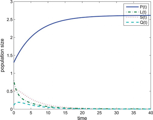
Figure 3. When $R_0<1$ and $\xi (\mathrm{\Lambda }+\mathrm{\Pi })/\mu >max\{\mu +d_i,i=1,2,3\}$, the problem drinking-free equilibrium $E_0$ of Equation (4(4) $\begin{array}{rl}\frac{\mathrm{d}P}{\mathrm{d}t}& =\mathrm{\Lambda }+\mathrm{\Pi }-\epsilon P-\xi PL-\alpha PS-\beta PQ-\mu P,\\ \frac{\mathrm{d}L}{\mathrm{d}t}& =\epsilon P+\xi PL+\alpha PS+\beta PQ+\rho Q-(\mu +d_1+\omega )L,\\ \frac{\mathrm{d}S}{\mathrm{d}t}& =(1-p)\omega L-(\mu +d_2+\phi )S,\\ \frac{\mathrm{d}Q}{\mathrm{d}t}& =p\omega L+\phi S-(\mu +d_3+\rho )Q.\end{array}$(4) ) is globally asymptotically stable.

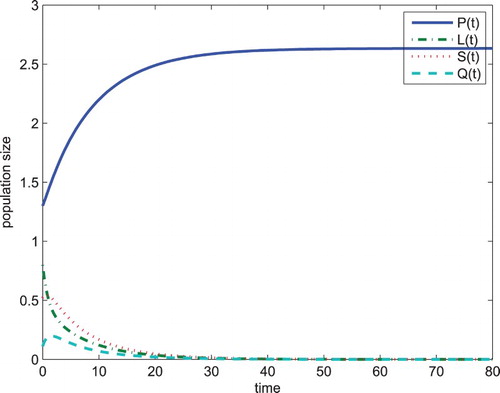
Figure 4. The problem drinking equilibrium $E^{\ast }$ of Equation (1(1) $\begin{array}{rl}\frac{\mathrm{d}P}{\mathrm{d}t}& =\mathrm{\Lambda }+(1-q_1-q_2)\mathrm{\Pi }-\epsilon P-\xi PL-\alpha PS-\beta PQ-\mu P,\\ \frac{\mathrm{d}L}{\mathrm{d}t}& =q_1\mathrm{\Pi }+\epsilon P+\xi PL+\alpha PS+\beta PQ+\rho Q-(\mu +d_1+\omega )L,\\ \frac{\mathrm{d}S}{\mathrm{d}t}& =q_2\mathrm{\Pi }+(1-p)\omega L-(\mu +d_2+\phi )S,\\ \frac{\mathrm{d}Q}{\mathrm{d}t}& =p\omega L+\phi S-(\mu +d_3+\rho )Q,\\ N& =P+L+S+Q,\end{array}$(1) ) is globally asymptotically stable.

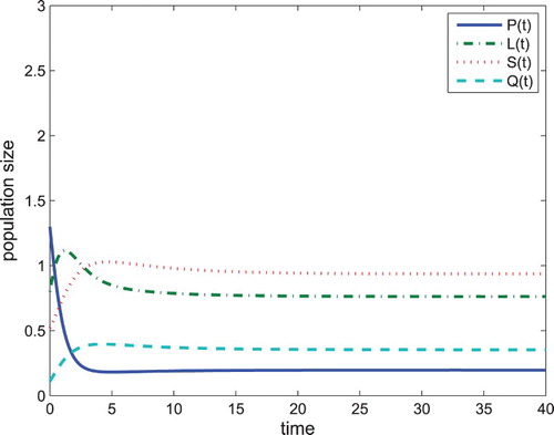
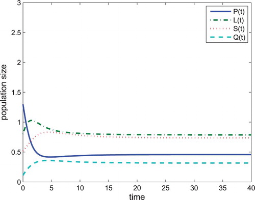
Figure 5. When $\epsilon =\xi =\alpha =0,\beta =0.5$, the problem drinking equilibrium $E^{\ast }$ of Equation (1(1) $\begin{array}{rl}\frac{\mathrm{d}P}{\mathrm{d}t}& =\mathrm{\Lambda }+(1-q_1-q_2)\mathrm{\Pi }-\epsilon P-\xi PL-\alpha PS-\beta PQ-\mu P,\\ \frac{\mathrm{d}L}{\mathrm{d}t}& =q_1\mathrm{\Pi }+\epsilon P+\xi PL+\alpha PS+\beta PQ+\rho Q-(\mu +d_1+\omega )L,\\ \frac{\mathrm{d}S}{\mathrm{d}t}& =q_2\mathrm{\Pi }+(1-p)\omega L-(\mu +d_2+\phi )S,\\ \frac{\mathrm{d}Q}{\mathrm{d}t}& =p\omega L+\phi S-(\mu +d_3+\rho )Q,\\ N& =P+L+S+Q,\end{array}$(1) ) is globally asymptotically stable.

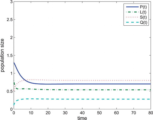
Figure 6. When $q_1=q_2=\epsilon =\alpha =\xi =0,\beta =0.5$, the problem drinking equilibrium $E^{\ast \ast }$ of Equation (4(4) $\begin{array}{rl}\frac{\mathrm{d}P}{\mathrm{d}t}& =\mathrm{\Lambda }+\mathrm{\Pi }-\epsilon P-\xi PL-\alpha PS-\beta PQ-\mu P,\\ \frac{\mathrm{d}L}{\mathrm{d}t}& =\epsilon P+\xi PL+\alpha PS+\beta PQ+\rho Q-(\mu +d_1+\omega )L,\\ \frac{\mathrm{d}S}{\mathrm{d}t}& =(1-p)\omega L-(\mu +d_2+\phi )S,\\ \frac{\mathrm{d}Q}{\mathrm{d}t}& =p\omega L+\phi S-(\mu +d_3+\rho )Q.\end{array}$(4) ) is globally asymptotically stable.

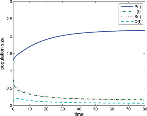
Figure 7. When $q_1=q_2=\epsilon =0$, the problem drinking equilibrium $E^{\ast \ast }$ of Equation (4(4) $\begin{array}{rl}\frac{\mathrm{d}P}{\mathrm{d}t}& =\mathrm{\Lambda }+\mathrm{\Pi }-\epsilon P-\xi PL-\alpha PS-\beta PQ-\mu P,\\ \frac{\mathrm{d}L}{\mathrm{d}t}& =\epsilon P+\xi PL+\alpha PS+\beta PQ+\rho Q-(\mu +d_1+\omega )L,\\ \frac{\mathrm{d}S}{\mathrm{d}t}& =(1-p)\omega L-(\mu +d_2+\phi )S,\\ \frac{\mathrm{d}Q}{\mathrm{d}t}& =p\omega L+\phi S-(\mu +d_3+\rho )Q.\end{array}$(4) ) is globally asymptotically stable.

If we use all the data in Table 2 and choose $q_1=0.4,q_2=0.3$. We can clearly see the problem drinking equilibrium $E^{\ast }$ of Equation (1(1) $\begin{array}{rl}\frac{\mathrm{d}P}{\mathrm{d}t}& =\mathrm{\Lambda }+(1-q_1-q_2)\mathrm{\Pi }-\epsilon P-\xi PL-\alpha PS-\beta PQ-\mu P,\\ \frac{\mathrm{d}L}{\mathrm{d}t}& =q_1\mathrm{\Pi }+\epsilon P+\xi PL+\alpha PS+\beta PQ+\rho Q-(\mu +d_1+\omega )L,\\ \frac{\mathrm{d}S}{\mathrm{d}t}& =q_2\mathrm{\Pi }+(1-p)\omega L-(\mu +d_2+\phi )S,\\ \frac{\mathrm{d}Q}{\mathrm{d}t}& =p\omega L+\phi S-(\mu +d_3+\rho )Q,\\ N& =P+L+S+Q,\end{array}$(1) ) is globally asymptotically stable (Figure 4). If we choose $\epsilon =\xi =\alpha =0,\beta =0.5$ and other data follow Table 2, we can see Theorem  3.4 is correct (Figure 5).

In the Figure 6, we perform numerical simulations to illustrate the result of Theorem 3.5. If $q_1=q_2=\epsilon =\alpha =\xi =0,\beta =0.5$ and other parameters follow Table 2, we can clearly see the problem drinking equilibrium $E^{\ast \ast }$ is globally asymptotically stable. If we only assume $q_1=q_2=\epsilon =0$, then $\xi \ne \alpha \ne 0$, we can also get the problem drinking equilibrium $E^{\ast \ast }$ is globally asymptotically stable (Figure 7).

5. Discussion

We have formulated a drinking model with constant immigration. We obtain the following results: if $q_1^2+q_2^2\ne 0$, system (1(1) $\begin{array}{rl}\frac{\mathrm{d}P}{\mathrm{d}t}& =\mathrm{\Lambda }+(1-q_1-q_2)\mathrm{\Pi }-\epsilon P-\xi PL-\alpha PS-\beta PQ-\mu P,\\ \frac{\mathrm{d}L}{\mathrm{d}t}& =q_1\mathrm{\Pi }+\epsilon P+\xi PL+\alpha PS+\beta PQ+\rho Q-(\mu +d_1+\omega )L,\\ \frac{\mathrm{d}S}{\mathrm{d}t}& =q_2\mathrm{\Pi }+(1-p)\omega L-(\mu +d_2+\phi )S,\\ \frac{\mathrm{d}Q}{\mathrm{d}t}& =p\omega L+\phi S-(\mu +d_3+\rho )Q,\\ N& =P+L+S+Q,\end{array}$(1) ) has no problem drinking-free equilibrium. That is, the drinking model (1(1) $\begin{array}{rl}\frac{\mathrm{d}P}{\mathrm{d}t}& =\mathrm{\Lambda }+(1-q_1-q_2)\mathrm{\Pi }-\epsilon P-\xi PL-\alpha PS-\beta PQ-\mu P,\\ \frac{\mathrm{d}L}{\mathrm{d}t}& =q_1\mathrm{\Pi }+\epsilon P+\xi PL+\alpha PS+\beta PQ+\rho Q-(\mu +d_1+\omega )L,\\ \frac{\mathrm{d}S}{\mathrm{d}t}& =q_2\mathrm{\Pi }+(1-p)\omega L-(\mu +d_2+\phi )S,\\ \frac{\mathrm{d}Q}{\mathrm{d}t}& =p\omega L+\phi S-(\mu +d_3+\rho )Q,\\ N& =P+L+S+Q,\end{array}$(1) ) does not have the state of problem drinking-free. System (1(1) $\begin{array}{rl}\frac{\mathrm{d}P}{\mathrm{d}t}& =\mathrm{\Lambda }+(1-q_1-q_2)\mathrm{\Pi }-\epsilon P-\xi PL-\alpha PS-\beta PQ-\mu P,\\ \frac{\mathrm{d}L}{\mathrm{d}t}& =q_1\mathrm{\Pi }+\epsilon P+\xi PL+\alpha PS+\beta PQ+\rho Q-(\mu +d_1+\omega )L,\\ \frac{\mathrm{d}S}{\mathrm{d}t}& =q_2\mathrm{\Pi }+(1-p)\omega L-(\mu +d_2+\phi )S,\\ \frac{\mathrm{d}Q}{\mathrm{d}t}& =p\omega L+\phi S-(\mu +d_3+\rho )Q,\\ N& =P+L+S+Q,\end{array}$(1) ) has a unique problem drinking equilibrium. By constructing Lyapunov function, we prove the global stability of the problem drinking equilibrium under certain conditions. However, if $q_1=q_2=\epsilon =0$, system (2.1) exists two equilibia, that is, problem drinking-free equilibrium and problem drinking equilibrium. By means of the next generation matrix [31], we obtain their basic reproduction number ${\mathcal{R}}_0$ which plays a crucial role. By constructing Lyapunov function, we prove the stability of all the equilibria under certain conditions.

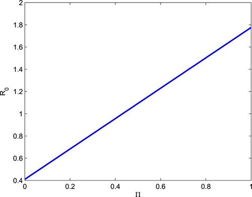
Many researchers [11, 36, 38] focus on the influence of parameters on the basic reproductive number. In this paper, we consider the effect of constant immigrants to alcohol problems. It is conceivable that when drinking immigrants increase, the number of alcoholics who are influenced by drinking immigrants will also increase. Hence, the basic reproduction number $R_0$ is increasing (Figure 8). Thus, we can draw the following conclusions: alcohol immigrants not only affect an area's drinking culture, but also increase the difficulty of the temperance work of the region. So we should restrict the alcoholics to immigrate in order to quit drinking.

Figure 8. The relationship among $R_0$ and Π.

Disclosure statement

No potential conflict of interest was reported by the authors.

Additional information

Funding

This work is supported by the NNSF of China [grant number 11461041], the NSF of Gansu Province [grant number 148RJZA024] and the Development Program for HongLiu Outstanding Young Teachers in Lanzhou University of Technology.

References

- C. Castillo-Chavez and B. Song, Dynamical models of tuberculosis and their applications, Math. Biosci. Eng. 1 (2004), pp. 361–404. doi: 10.3934/mbe.2004.1.361
- Centers for Disease Control and Prevention, Department of Health and Human Services, Atlanta. Available at http://www.cdc.gov/alcohol/faqs.htm, last accessed March 11, 2009.
- A. Cintrón-Arias, F. Sánchez, X.H. Wang, C. Castillo-Chavez, D.M. Gorman, and P.J. Gruenewald, The role of nonlinear relapse on contagion amongst drinking communities. in Mathematical and Statistical Estimation Approaches in Epidemiology, G. Chowell, J.M. Hayman, L.M.A. Bettencourt, and D. Bies, eds., Springer, New York, NY, 2009, pp. 343–360.
- C.M. Gibson-Davis and J. Brooks-Gunn, Couples' immigration status and ethnicity as determinants of breastfeeding, Am. J. Public Health 96(8) (2006), pp. 641–646. doi: 10.2105/AJPH.2005.064840
- Global Status Report on Alcohol and Health. Available at http://www.who.int/.
- H.F. Huo, R. Chen, and X.Y. Wang, Modelling and stability of HIV/AIDS epidemic model with treatment, Appl. Math. Model. 40 (2016), pp. 6550–6559. doi: 10.1016/j.apm.2016.01.054
- H.F. Huo, S.J. Dang, and Y.N. Li, Stability of a two-strain tuberculosis model with general contact rate, Abs. Appl. Anal. 2010 (2010), pp. 293747 (31 pages).
- H.F. Huo and L.X. Feng, Global stability for an HIV/AIDS epidemic model with different latent stages and treatment, Appl. Math. Model. 37 (2013), pp. 1480–1489. doi: 10.1016/j.apm.2012.04.013
- H.F. Huo and N.N. Song, Global stability for a binge drinking model with two-stage, Discrete Dyn. Nat. Soc., 2012, Article ID 530267, 14 pages.
- H.F. Huo and X.M. Zhang, Complex dynamics in an alcoholism model with the impact of Twitter, Math. Biosci. 281 (2016), pp. 24–35. doi: 10.1016/j.mbs.2016.08.009
- H.F. Huo and C.C. Zhu, Influence of relapse in a giving up smoking model, Abs. Appl. Anal. 2013 (2013), pp. 525461 (12 pages).
- H.F. Huo and M.X. Zou, Modelling effects of treatment at home on tuberculosis transmission dynamics, Appl. Math. Model. 40 (2016), pp. 9474–9484. doi: 10.1016/j.apm.2016.06.029
- Investigation Report on the Status of Chinese Public Health Drink, 2007. Available at http://wenku.baidu.com/view/25266a2eb4daa58da0114a03.html/.
- A. Korobeinikov, Global properties of basic virus dynamics models, Bull. Math. Biol. 66 (2004), pp. 879–883. doi: 10.1016/j.bulm.2004.02.001
- J.P. LaSalle, The Stability of Dynamical Systems, Region Conference Series in Applied Mathematics, SIAM, Philadelphia, PA, 1976.
- S. Lee, E. Jung, and C. Castillo-Chavez, Optimal control intervention strategies in low- and high-risk problem drinking populations, Socio-Econ. Plan. Sci. 44 (2010), pp. 258–265. doi: 10.1016/j.seps.2010.07.006
- T. Lillebaek, A.B. Andersen, A. Dirksen, and E. Smith, Persistent high incidence of tuberculosis in immigrants in a low-incidence country, Emerg. Infect. Dis. 8(7) (2002), pp. 679–684. doi: 10.3201/eid0807.010482
- M.E. McPherson, H. Kelly, M.S. Patel, and D. Leslie, Persistent risk of tuberculosis in migrants a decade after arrival in Australia, Med. J. Aust. 188 (2008), pp. 528–531.
- A. Mubayi, P.E. Greenwood, C. Castillo-Garsow, P.J. Gruenewald, and D.M. Gorman, The impact of relative residence times on the distribution of heavy drinkers in highly distinct environments, Socio-Econ. Plan. Sci. 44 (2010), pp. 45–56. doi: 10.1016/j.seps.2009.02.002
- G. Mulone and B. Straughan, Modeling binge drinking, Int. J. Biomath. 5(1) (2012), pp. 1250005 (14 pages). doi: 10.1142/S1793524511001453
- S. Mushayabasa and C.P. Bhunu, Modelling the effects of heavy alcohol consumption on the transmission dynamics of gonorrhea, Nonlinear Dyn. 66 (2011), pp. 695–706. doi: 10.1007/s11071-011-9942-4
- National Institute on Alcohol Abuse and Alcoholism, Department of Health and Human Services, United States of America. Available at http://www.niaaa.nih.gov/FAQs/General-English/, last accessed March 11, 2009.
- R. Qesmi, J. Wu, J.H. Wu, and J.M. Heffernan, Influence of backward bifurcation in a model of hepatitis B and C viruses, Math. Biosci. 224 (2010), pp. 118–125. doi: 10.1016/j.mbs.2010.01.002
- N. Rice, R. Carr-hill, P. Dixon, and M. Sutton, The influence of households on drinking behaviour: A multilevel analysis, Soc. Sci. Med. 46(8) (1998), pp. 971–979. doi: 10.1016/S0277-9536(97)10017-X
- O. Sharomi and A.B. Gumel, Curtailing smoking dynamics: A mathematical modeling approach, Appl. Math. Comput. 195 (2008), pp. 475–499.
- F. S'anchez, X. Wang, C. Castillo-Chavez, D.M. Gorman, and P.J. Gruenewald, Drinking as an epidemic—A simple mathematical model with recovery and relapse, in Therapist's Guide to Evidence-based Relapse Prevention: Practical Resources for the Mental Health Professional, K.A. Witkiewitz and G.A. Marlatt, eds., Academic, Burlington, NJ, 2007, pp. 353–368.
- M.O. Souza and J.P. Zubelli, Global stability for a class of virus models with cytotoxoc t lymphocyte immune response and antigenic variation, Bull. Math. Biol. 73 (2011), pp. 609–625. doi: 10.1007/s11538-010-9543-2
- R. Thadhani, C.A. Camargo, M.J. Stampfer, G.C. Curhan, W.C. Willett, and E.B. Rimm, Prospective study of moderate alcohol consumption and risk of hypertension in young women, Arch. Intern. Med. 162(5) (2002), pp. 569–574. doi: 10.1001/archinte.162.5.569
- G. Thomas and E.M. Lungu, The influence of heavy alcohol consumption on HIV infection and progression, J. Biol. Syst. 17(4) (2009), pp. 685–712. doi: 10.1142/S0218339009003083
- G. Thomas and E.M. Lungu, A two-sex model for the influence of heavy alcohol consumption on the spread of HIV/AIDS, Math. Biosci. Eng. 7(4) (2010), pp. 871–904. doi: 10.3934/mbe.2010.7.871
- P. van den Driessche and J. Watmough, Reproduction numbers and sub-threshold endemic equilibra for compartmental models of disease transmission, Math. Biosci. 180 (2002), pp. 29–48. doi: 10.1016/S0025-5564(02)00108-6
- X.-Y. Wang, K. Hattaf, H.-F. Huo, and H. Xiang. Stability analysis of a delayed social epidemics model with general contact rate and its optimal control, J. Ind. Manage. Optim. 12(4) (2016), pp. 1267–1285. doi: 10.3934/jimo.2016.12.1267
- World Health Statistics, 2013. Available at http://www.who.int/gho/publications/world_health_statistics/2013/en/.
- H. Xiang, Y.L. Tang, and H.F. Huo, A viral model with intracellular delay and humoral immunity, Bull. Malaysian Math. Sci. Soc. (2016). doi: 10.1007/s40840-016-0326-2.
- H. Xiang, N.N. Song, and H.F. Huo, Modelling effects of public health educational campaigns on drinking dynamics, J. Biol. Dyn. 10(1) (2016), pp. 164–178. doi: 10.1080/17513758.2015.1115562
- H. Xiang, C.C. Zhu, and H.F. Huo, Global stability of a quit drinking model with relapse, J. Biomath. 31 (2016), pp. 15–27.
- R. Xu, Global stability of an HIV-1 infection model with saturation infection and intracellular delay, J. Math. Anal. Appl. 375 (2011), pp. 75–81. doi: 10.1016/j.jmaa.2010.08.055
- C.C. Zhu, W.T. Li, and F.Y. Yang, Traveling waves of a reaction–diffusion SIRQ epidemic model with relapse, J. Appl. Anal. Comput. 7 (2017), pp. 147–171.
- E. Ziv, C.L. Daley, and S.M. Blower, Early therapy for latent tuberculosis infection, Am. J. Epidemiol. 153 (2001), pp. 381–385. doi: 10.1093/aje/153.4.381