How noise and coupling influence leading indicators of population extinction in a spatially extended ecological system

ABSTRACT

Anticipating critical transitions in spatially extended systems is a key topic of interest to ecologists. Gradually declining metapopulations are an important example of a spatially extended biological system that may exhibit a critical transition. Theory for spatially extended systems approaching extinction that accounts for environmental stochasticity and coupling is currently lacking. Here, we develop spatially implicit two-patch models with additive and multiplicative forms of environmental stochasticity that are slowly forced through population collapse, through changing environmental conditions. We derive patch-specific expressions for candidate indicators of extinction and test their performance via a simulation study. Coupling and spatial heterogeneities decrease the magnitude of the proposed indicators in coupled populations relative to isolated populations, and the noise regime and the degree of coupling together determine trends in summary statistics. This theory may be readily applied to other spatially extended ecological systems, such as coupled infectious disease systems on the verge of elimination.

KEYWORDS:

• Early warning signals
• environmental stochasticity
• transcritical bifurcation
• metapopulation
• population collapse

AMS SUBJECT CLASSIFICATION:

• 92B05

1. Introduction

Understanding and predicting critical transitions in complex systems, where a system shifts from one dynamical state to another, is a key research topic in a wide range of fields [38], including ecology [7, 9, 40], financial systems [4, 19, 37], climate science [30] and medicine (e.g. [27, 36, 44, 46]). Certain types of critical transitions can be represented mathematically as bifurcations if the change in the external forcing variable is slow relative to internal system variables. A sudden drastic change from one state to another, distant, state may be characterized by a fold or saddle-node bifurcation, whereas a smooth, gradual change in system state, where states meet and exchange stability, can be expressed as a transcritical bifurcation. For example, in ecology, populations subject to Allee effects may be described in terms of saddle-node bifurcations, whereas logistically growing populations on the verge of extinction are often characterized by transcritical bifurcations.

The gradual loss of stability is a key property of systems close to a bifurcation point. As the bifurcation point is approached, system perturbations take longer to return to equilibrium. This phenomenon has been termed ‘critical slowing down’ [42, 47, 50]. The return rate of the system to the steady state is characterized by the magnitude of the dominant eigenvalue of the linearization matrix, which approaches zero as the system approaches criticality. In ecology, critical slowing down is one measure of resilience, the ability of a system to withstand disturbances [38, 40]. What is interesting is that bifurcations can be potentially anticipated by identifying critical slowing down through statistical analysis of temporal and spatial patterns in data [38]. Temporal summary statistics such as lag-1 autocorrelation, variance and skewness have been used to predict impending bifurcations through identification of critical slowing down in simulated data to test their usefulness as part of early warning systems for critical transitions [14]. Temporal statistics can be derived in terms of the parameters of linearized stochastic differential equation models [17, 33] and through linearized systems of difference equations (known as autoregressive models in the time series literature), for example, [22, 23, 39], but theory for multidimensional systems approaching critical transitions, subject to different noise regimes other than additive, is not well-developed (but see [34, 35] for derivations of temporal statistics for two-dimensional infectious disease systems subject to demographic stochasticity).

Spatial systems are multi-dimensional, and it is not well understood how spatial interactions, such as movement between patches, synchronous environmental fluctuations (Moran effects), spatial heterogeneities and rescue effects through dispersal affect predictability of critical transitions in spatially extended systems. Bel et al. [6] explored how the existence of Maxwell points affect the nature of a transition in a spatial system. Villa Martin et al. [49] increased the intensities of demographic noise, coupling and spatial heterogeneity to show the nature of the critical transition in a stochastic partial differential equation can be altered from abrupt to gradual. Both of these studies used stochastic reaction–diffusion equations to investigate the dynamics of spatiotemporal systems near criticality. Alternatively, dynamical systems on networks have been used to account for interactions between spatial structure and criticality (e.g. [41, 43]). Clearly, any early warning system devised for spatially extended systems needs to account for these complexities. Numerous spatial summary statistics have been proposed as leading indicators of transitions [25]. Guttal and Jayaprakash [18] studied the performance of spatial statistics such as spatial variance and spatial skewness as indicators of vegetation population collapse due to increased grazing pressure. Dakos et al. [13] investigated spatial correlation as an indicator of transitions, while Dai et al. [10] proposed the recovery length indicator as a measure of propensity to transition in spatially extended systems. However, spatial statistics are not calculated from time series; rather, they are computed from ‘spatial snapshots’ of the system at specific times (e.g. [8]). Spatial statistics average over dynamics within patches, which might not be as accurate if dispersal is small, or if environmental conditions are heterogeneous. The loss of accuracy may be particularly important if different biotic or abiotic variables are changing with time in some patches but not in others, and how their influence propagates through the system might be more accurately assessed using patch-specific indicators. Additionally, from a mathematical perspective, spatial statistics do not usually have analytical expressions in terms of the parameters of a model. Consequently, temporal indicators that are specific to each patch are needed, in addition to spatial statistics, to anticipate transitions in spatially extended systems.

To understand how critical slowing down manifests in a multi-patch system, analytical predictions for temporal statistics summarizing variability and slowing down properties in each patch are required. For example, to empirically assess predictability of metapopulation extinction, Dai et al. [10] conducted a multi-patch yeast population experiment that coupled separate populations through transferral of yeast between patches. They showed that increasing the degree of coupling decreased the magnitude of temporal early warning signals of collapse of the metapopulation relative to the isolated subpopulations. Each beaker containing yeast was a patch in the metapopulation. They speculated that transfer between patches ‘smooths out’ the stochastic fluctuations, and used discrete-time autoregressive models with additive noise to show that temporal signals are smaller in connected populations than in isolated populations. However, their approach assumed only additive noise, and they did not delineate how noise and coupling interact to determine statistical patterns in time series. Patch-specific predictions can additionally be used to answer questions such as whether a single patch can have a clear signal of an impending bifurcation, or whether all patches need to be monitored. A predictive theory for temporal statistics of spatially extended systems that accounts for environmental stochasticity and coupling is currently lacking.

To address this gap, we model a logistically growing metapopulation as a continuous system of two patches, where each subpopulation is gradually approaching extinction as a result of intrinsic patch parameters changing over long time scales. Gradually declining metapopulations on the verge of collapse are an important example of a spatially extended biological system that can exhibit a critical transition. Mathematically, a metapopulation that grows logistically at the local level is characterized by a transcritical bifurcation at the point of extinction. We focus on a smooth transition to extinction in this paper, as this type of transition is important for logistically growing populations approaching extinction [15, 20], and for susceptible-infectious-susceptible model infectious disease systems on the verge of elimination due to control activities that lessen transmission or quicken recovery [34]. We address the question of whether temporal statistics for subpopulation fluctuations can provide information on whether a two-patch metapopulation is losing stability, and consequently becoming closer to extinction. We use the model to show analytically that strong coupling suppresses temporal early warning signals in coupled homogeneous populations relative to isolated populations, and we test the predictions through a simulation study. We additionally extend the framework to study the effect of spatial heterogeneities on predicting extinction. Finally, we explore whether both patches exhibit early warning signals of extinction, or whether a single patch can be monitored. Our results suggest that critical slowing down is detectable in both patches, and we recommend they should be monitored simultaneously.

2. Model

2.1. Basic spatial model

Consider the following general model for a spatially extended population occupying two patches, (1) $\begin{array}{rl}\frac{\mathrm{d}{x}_1}{\mathrm{d}t}& =r_1{x}_1-x_1^2-m{x}_1+m{x}_2,\\ \frac{\mathrm{d}{x}_2}{\mathrm{d}t}& =r_2{x}_2-x_2^2-m{x}_2+m{x}_1,\end{array}$(1) where $x_i\ge 0$, i=1,2, denotes the density of subpopulation i that occupy patch i. In the absence of dispersal, subpopulation dynamics are determined by logistic growth at rate $r_i{x}_i-x_i^2$ in each patch. The model assumes that individuals migrate from patch i into patch j at rate $m{x}_i$. If the coupling strength m is positive, then a fraction m of subpopulation i disperse into the alternative patch. Population dynamics in each patch are determined by local environmental conditions, and we assume that local patch conditions affect the intrinsic growth rate of subpopulation i in each patch ($r_i\ge 0$). In the absence of dispersal, if $r_i>0$, net reproduction is greater than net mortality in each patch, and in ecological terms, each patch is a ‘source’. The model allows for homogeneous environmental conditions ($r_1=r_2=r$) and spatial heterogeneity in intrinsic dynamics ($r_1\ne r_2$). The spatially heterogeneous model has a positive steady state $(x_1^{\ast },x_2^{\ast })$ that can be determined numerically.

In the absence of coupling, each population is isolated, and each patch has two steady states. If $r_i>0$, each population i has a positive, locally stable steady state at $x_i=r_i$, and the population extinction state $x_i=0$ is unstable. At $r_i=0$, the two steady states meet and exchange stability, and a transcritical bifurcation occurs.

If environmental conditions are homogeneous (i.e. $r_1=r_2=r>0$) and the subpopulations move between the patches at rate m>0, the spatially extended system has two steady states: a positive steady state $(x_1^{\ast },x_2^{\ast })=(r,r)$ and an extinction state $(0,0)$. These steady states are spatially homogeneous because the population density is the same in each patch. The eigenvalues of the spatially homogeneous system (1(1) $\begin{array}{rl}\frac{\mathrm{d}{x}_1}{\mathrm{d}t}& =r_1{x}_1-x_1^2-m{x}_1+m{x}_2,\\ \frac{\mathrm{d}{x}_2}{\mathrm{d}t}& =r_2{x}_2-x_2^2-m{x}_2+m{x}_1,\end{array}$(1) ) are $-r$ and $-r-2m$ (e.g. [24]). If environmental conditions deteriorate in both patches, we assume that r declines towards zero. Consequently, the magnitude of both eigenvalues will decrease, and extinction will occur in both patches when the dominant eigenvalue $-r$ is equal to zero. Therefore, critical slowing down prior to population extinction is predicted in the spatially homogeneous system.

2.2. Fast-slow models

To capture the decline of the metapopulation towards extinction due to progressively worsening environmental conditions, a fast-slow model is needed to describe the dynamic approach to the transcritical bifurcation point. To model the effect of deteriorating environmental conditions and subsequent approach to population extinction in a spatially homogeneous system, we assume the intrinsic growth rate r declines slowly relative to the population dynamics in each patch. We modify model (1(1) $\begin{array}{rl}\frac{\mathrm{d}{x}_1}{\mathrm{d}t}& =r_1{x}_1-x_1^2-m{x}_1+m{x}_2,\\ \frac{\mathrm{d}{x}_2}{\mathrm{d}t}& =r_2{x}_2-x_2^2-m{x}_2+m{x}_1,\end{array}$(1) ) to allow for slowly changing environmental conditions, (2) $\begin{array}{rl}\frac{\mathrm{d}{x}_1}{\mathrm{d}t}& =r{x}_1-x_1^2-m{x}_1+m{x}_2,\\ \frac{\mathrm{d}{x}_2}{\mathrm{d}t}& =r{x}_2-x_2^2-m{x}_2+m{x}_1,\\ \frac{\mathrm{d}r}{\mathrm{d}t}& =-r_0,\end{array}$(2) where $r_0>0$ determines the rate of change of the intrinsic growth rate r in each patch. By Fenichel's Theorem [16, 29], in the limit $r_0\to 0$, trajectories of system (2(2) $\begin{array}{rl}\frac{\mathrm{d}{x}_1}{\mathrm{d}t}& =r{x}_1-x_1^2-m{x}_1+m{x}_2,\\ \frac{\mathrm{d}{x}_2}{\mathrm{d}t}& =r{x}_2-x_2^2-m{x}_2+m{x}_1,\\ \frac{\mathrm{d}r}{\mathrm{d}t}& =-r_0,\end{array}$(2) ) approach those of the model where r is constant. Since r evolves over a longer time scale relative to the population dynamics, we assume $0<r_0<<1$, and deteriorating conditions cause a linear decline in r, (3) $r\left(t\right)=\{\begin{array}{ll}r-r_{0}t,& t<t^{\ast },\\ 0,& t\ge t^{\ast },\end{array}$(3) where $t^{\ast }=r/r_0$ denotes the time that $r\left(t\right)$ becomes zero, which is an estimate for the time that the solution of model (2(2) $\begin{array}{rl}\frac{\mathrm{d}{x}_1}{\mathrm{d}t}& =r{x}_1-x_1^2-m{x}_1+m{x}_2,\\ \frac{\mathrm{d}{x}_2}{\mathrm{d}t}& =r{x}_2-x_2^2-m{x}_2+m{x}_1,\\ \frac{\mathrm{d}r}{\mathrm{d}t}& =-r_0,\end{array}$(2) ) and (3(3) $r\left(t\right)=\{\begin{array}{ll}r-r_{0}t,& t<t^{\ast },\\ 0,& t\ge t^{\ast },\end{array}$(3) ) reaches $(0,0)$.

In spatially heterogeneous systems, the environmental conditions that affect patch quality (e.g. resource availability) may vary. Consequently, the population dynamics in each patch may be governed by different intrinsic growth rates. Here, we assume environmental conditions remain constant in patch 1, (i.e. the growth rate $r_1$ remains positive and constant) but conditions deteriorate in patch 2, decreasing the growth rate of the population in that patch. These assumptions yield the following model, (4) $\begin{array}{rl}\frac{\mathrm{d}{x}_1}{\mathrm{d}t}& =r_1{x}_1-x_1^2-m{x}_1+m{x}_2,\\ \frac{\mathrm{d}{x}_2}{\mathrm{d}t}& =r_2{x}_2-x_2^2-m{x}_2+m{x}_1,\\ \frac{\mathrm{d}{r}_2}{\mathrm{d}t}& =-r_0,\end{array}$(4) and conditions induce a linear deterioration in the intrinsic growth rate of patch 2, (5) $r_2\left(t\right)=\{\begin{array}{ll}{r}_2-r_{0}t,& t<t^{\ast },\\ 0,& t\ge t^{\ast },\end{array}$(5) where $t^{\ast }$ denotes the time that $r_2\left(t\right)$ reaches zero. By Fenichel's theorem [16, 29], for sufficiently small $r_0$, the dynamics of the fast-slow system will approach those of the system where $r_2$ is constant. Models (2(2) $\begin{array}{rl}\frac{\mathrm{d}{x}_1}{\mathrm{d}t}& =r{x}_1-x_1^2-m{x}_1+m{x}_2,\\ \frac{\mathrm{d}{x}_2}{\mathrm{d}t}& =r{x}_2-x_2^2-m{x}_2+m{x}_1,\\ \frac{\mathrm{d}r}{\mathrm{d}t}& =-r_0,\end{array}$(2) ) and (4(4) $\begin{array}{rl}\frac{\mathrm{d}{x}_1}{\mathrm{d}t}& =r_1{x}_1-x_1^2-m{x}_1+m{x}_2,\\ \frac{\mathrm{d}{x}_2}{\mathrm{d}t}& =r_2{x}_2-x_2^2-m{x}_2+m{x}_1,\\ \frac{\mathrm{d}{r}_2}{\mathrm{d}t}& =-r_0,\end{array}$(4) ) can be expressed as (6) $\begin{array}{rl}\frac{\mathrm{d}{x}_1}{\mathrm{d}t}& =r_1\left(t\right)x_1-x_1^2-m{x}_1+m{x}_2,\\ \frac{\mathrm{d}{x}_2}{\mathrm{d}t}& =r_2\left(t\right)x_2-x_2^2-m{x}_2+m{x}_1,\end{array}$(6) where $r_1\left(t\right)=r_2\left(t\right)=r\left(t\right)$ in the spatially homogeneous case (Equations (2(2) $\begin{array}{rl}\frac{\mathrm{d}{x}_1}{\mathrm{d}t}& =r{x}_1-x_1^2-m{x}_1+m{x}_2,\\ \frac{\mathrm{d}{x}_2}{\mathrm{d}t}& =r{x}_2-x_2^2-m{x}_2+m{x}_1,\\ \frac{\mathrm{d}r}{\mathrm{d}t}& =-r_0,\end{array}$(2) ) and (3(3) $r\left(t\right)=\{\begin{array}{ll}r-r_{0}t,& t<t^{\ast },\\ 0,& t\ge t^{\ast },\end{array}$(3) )). In the spatially heterogeneous case, we assume $r_1\left(t\right)=r_1>0$ and $r_2\left(t\right)$ is given by Equation (5(5) $r_2\left(t\right)=\{\begin{array}{ll}{r}_2-r_{0}t,& t<t^{\ast },\\ 0,& t\ge t^{\ast },\end{array}$(5) ).

2.3. Stochastic models

Environmental conditions may fluctuate due to variation in climate and weather patterns such as humidity and precipitation, and population dynamics in each patch are sensitive to random fluctuations. We derive systems of Ito stochastic differential equations describing spatially homogeneous metapopulations by assuming that environmental stochasticity can influence patch dynamics through two different mechanisms.

2.3.1. Additive noise

The assumption of additive environmental noise implies that environmental variation affects the change in population density as a whole in each patch. In a small time increment $\mathrm{\Delta }t$, we assume the change in population density $\mathrm{\Delta }{x}_i$ in each patch fluctuates randomly according to a normal distribution with mean $\left(r_i\right(t)x_i-x_i^2-m{x}_i+m{x}_j)\mathrm{\Delta }t$ and variance ${\sigma }_a^2\mathrm{\Delta }t$, (7) $\mathrm{\Delta }{x}_i\sim \mathrm{Normal}\left\{\right(r_i\left(t\right)x_i-x_i^2-m{x}_i+m{x}_j)\mathrm{\Delta }t,{\sigma }_a^2\mathrm{\Delta }t\}.$(7) The strength of noise ${\sigma }_a$ is assumed to be equal in each patch, and environmental variations are uncorrelated in space (e.g. the noise level does not decay with distance between patches) and in time (random fluctuations in population density $x_1$ do not covary with fluctuations in $x_2$). We can express (7(7) $\mathrm{\Delta }{x}_i\sim \mathrm{Normal}\left\{\right(r_i\left(t\right)x_i-x_i^2-m{x}_i+m{x}_j)\mathrm{\Delta }t,{\sigma }_a^2\mathrm{\Delta }t\}.$(7) ) as a system of equations, (8) $\begin{array}{rl}{x}_1(t+\mathrm{\Delta }t)-x_1\left(t\right)& =\left(r_1\right(t)x_1-x_1^2-m{x}_1+m{x}_2)\mathrm{\Delta }t+{\sigma }_a\sqrt{\mathrm{\Delta }t}{\eta }_1,\\ x_2(t+\mathrm{\Delta }t)-x_2\left(t\right)& =\left(r_2\right(t)x_2-x_2^2-m{x}_2+m{x}_1))\mathrm{\Delta }t+{\sigma }_a\sqrt{\mathrm{\Delta }t}{\eta }_2,\end{array}$(8) where ${\eta }_i$ are normal random variables with mean zero and unit variance. If $\mathrm{\Delta }t\to 0$ and assuming the stochastic integral exists and is unique, then ${\eta }_i\sqrt{\mathrm{\Delta }t}\to \mathrm{d}{W}_i\left(t\right)$, where $\mathrm{d}{W}_i\left(t\right)$ is a Wiener process [2]. Equations (8(8) $\begin{array}{rl}{x}_1(t+\mathrm{\Delta }t)-x_1\left(t\right)& =\left(r_1\right(t)x_1-x_1^2-m{x}_1+m{x}_2)\mathrm{\Delta }t+{\sigma }_a\sqrt{\mathrm{\Delta }t}{\eta }_1,\\ x_2(t+\mathrm{\Delta }t)-x_2\left(t\right)& =\left(r_2\right(t)x_2-x_2^2-m{x}_2+m{x}_1))\mathrm{\Delta }t+{\sigma }_a\sqrt{\mathrm{\Delta }t}{\eta }_2,\end{array}$(8) ) converge in the mean square sense to the system of stochastic differential equations, (9) $\begin{array}{rl}\mathrm{d}{x}_1& =\left(r_1\right(t)x_1-x_1^2-m{x}_1+m{x}_2)\mathrm{d}t+{\sigma }_a\mathrm{d}{W}_1,\\ \mathrm{d}{x}_2& =\left(r_2\right(t)x_2-x_2^2-m{x}_2+m{x}_1))\mathrm{d}t+{\sigma }_a\mathrm{d}{W}_2.\end{array}$(9) System (9(9) $\begin{array}{rl}\mathrm{d}{x}_1& =\left(r_1\right(t)x_1-x_1^2-m{x}_1+m{x}_2)\mathrm{d}t+{\sigma }_a\mathrm{d}{W}_1,\\ \mathrm{d}{x}_2& =\left(r_2\right(t)x_2-x_2^2-m{x}_2+m{x}_1))\mathrm{d}t+{\sigma }_a\mathrm{d}{W}_2.\end{array}$(9) ) is a stochastic analogue of the fast-slow system (6(6) $\begin{array}{rl}\frac{\mathrm{d}{x}_1}{\mathrm{d}t}& =r_1\left(t\right)x_1-x_1^2-m{x}_1+m{x}_2,\\ \frac{\mathrm{d}{x}_2}{\mathrm{d}t}& =r_2\left(t\right)x_2-x_2^2-m{x}_2+m{x}_1,\end{array}$(6) ).

2.3.2. Mechanistic $($multiplicative$)$ noise

Model (9(9) $\begin{array}{rl}\mathrm{d}{x}_1& =\left(r_1\right(t)x_1-x_1^2-m{x}_1+m{x}_2)\mathrm{d}t+{\sigma }_a\mathrm{d}{W}_1,\\ \mathrm{d}{x}_2& =\left(r_2\right(t)x_2-x_2^2-m{x}_2+m{x}_1))\mathrm{d}t+{\sigma }_a\mathrm{d}{W}_2.\end{array}$(9) ) assumes the patch growth rate is affected by environmental variation by a non-specific mechanism. Here we derive an alternative stochastic fast-slow model. In a small time increment $\mathrm{\Delta }t$, the intrinsic growth rate in each patch is influenced by random environmental fluctuations that are normally distributed with mean $r_i\left(t\right)\mathrm{\Delta }t$ and variance ${\sigma }_{\mu }^2\mathrm{\Delta }t$, (10) $r_i\left(t\right)\mathrm{\Delta }t\sim \mathrm{Normal}\left\{r_i\right(t)\mathrm{\Delta }t,{\sigma }_{\mu }^2\mathrm{\Delta }t\}.$(10) The strength of noise ${\sigma }_{\mu }$ is assumed to be equal in each patch, and environmental variations are uncorrelated in space and time. Noting that Equation (10(10) $r_i\left(t\right)\mathrm{\Delta }t\sim \mathrm{Normal}\left\{r_i\right(t)\mathrm{\Delta }t,{\sigma }_{\mu }^2\mathrm{\Delta }t\}.$(10) ) can be written as $r_i\left(t\right)\mathrm{\Delta }t+{\sigma }_{\mu }\sqrt{\mathrm{\Delta }t}{\eta }_i$, where ${\eta }_i$ are independent normally distributed random variables with mean zero and unit variance, we can write down the following system of equations that describe the change in population densities in a small increment $\mathrm{\Delta }t$, (11) $\begin{array}{rl}{x}_1(t+\mathrm{\Delta }t)-x_1\left(t\right)& =\left(r_1\right(t)x_1-x_1^2-m{x}_1+m{x}_2)\mathrm{\Delta }t+{\sigma }_{\mu }{x}_1\sqrt{\mathrm{\Delta }t}{\eta }_1,\\ x_2(t+\mathrm{\Delta }t)-x_2\left(t\right)& =\left(r_2\right(t)x_2-x_2^2-m{x}_2+m{x}_1))\mathrm{\Delta }t+{\sigma }_{\mu }{x}_2\sqrt{\mathrm{\Delta }t}{\eta }_2.\end{array}$(11)

If $\mathrm{\Delta }t\to 0$ and assuming the stochastic integral exists and is unique, then ${\eta }_i\sqrt{\mathrm{\Delta }t}\to \mathrm{d}{W}_i\left(t\right)$, where $\mathrm{d}{W}_i\left(t\right)$ is a Wiener process [2]. Equations (8(8) $\begin{array}{rl}{x}_1(t+\mathrm{\Delta }t)-x_1\left(t\right)& =\left(r_1\right(t)x_1-x_1^2-m{x}_1+m{x}_2)\mathrm{\Delta }t+{\sigma }_a\sqrt{\mathrm{\Delta }t}{\eta }_1,\\ x_2(t+\mathrm{\Delta }t)-x_2\left(t\right)& =\left(r_2\right(t)x_2-x_2^2-m{x}_2+m{x}_1))\mathrm{\Delta }t+{\sigma }_a\sqrt{\mathrm{\Delta }t}{\eta }_2,\end{array}$(8) ) converges in the mean square sense to the system of stochastic differential equations, (12) $\begin{array}{rl}\mathrm{d}{x}_1& =\left(r_1\right(t)x_1-x_1^2-m{x}_1+m{x}_2)\mathrm{d}t+{\sigma }_{\mu }{x}_1\mathrm{d}{W}_1,\\ \mathrm{d}{x}_2& =\left(r_2\right(t)x_2-x_2^2-m{x}_2+m{x}_1))\mathrm{d}t+{\sigma }_{\mu }{x}_2\mathrm{d}{W}_2.\end{array}$(12) Since random perturbations scale with the population density $x_i$ in each patch, system (12(12) $\begin{array}{rl}\mathrm{d}{x}_1& =\left(r_1\right(t)x_1-x_1^2-m{x}_1+m{x}_2)\mathrm{d}t+{\sigma }_{\mu }{x}_1\mathrm{d}{W}_1,\\ \mathrm{d}{x}_2& =\left(r_2\right(t)x_2-x_2^2-m{x}_2+m{x}_1))\mathrm{d}t+{\sigma }_{\mu }{x}_2\mathrm{d}{W}_2.\end{array}$(12) ) describes a multiplicative noise model. We call model (12(12) $\begin{array}{rl}\mathrm{d}{x}_1& =\left(r_1\right(t)x_1-x_1^2-m{x}_1+m{x}_2)\mathrm{d}t+{\sigma }_{\mu }{x}_1\mathrm{d}{W}_1,\\ \mathrm{d}{x}_2& =\left(r_2\right(t)x_2-x_2^2-m{x}_2+m{x}_1))\mathrm{d}t+{\sigma }_{\mu }{x}_2\mathrm{d}{W}_2.\end{array}$(12) ) mechanistic because uncorrelated environmental variations of equal strength are assumed to specifically affect the intrinsic growth rate of each subpopulation.

2.3.3. Numerical simulations of the homogeneous stochastic models

To examine the behaviour of the stochastic fast-slow models as extinction is approached, we simulated the models using the parameters in Table 1. Figure 1 shows realizations of the $x_1$ subpopulation in isolated patches (m=0) (Figure 1(a, d)) compared to simulations of systems where the $x_1$ population is coupled to another patch, under low and high dispersal, subject to the contrasting noise regimes, and with homogeneous environmental conditions. Under both noise regimes, coupling patches through migration dampens environmental fluctuations in each patch, compared to when the patches are isolated. When coupling is low, and intrinsic dynamics are equal in each patch, coupled populations fluctuate on a similar level to isolated populations (e.g. compare Figure 1(a, b)). When coupling is high, it is evident from the simulations that fluctuations are dampened due to the influence of coupling. These observations are independent of the type of noise. When noise is mechanistic, the $x_1$ population appears to be less likely to go extinct, since the noise level tracks the equilibrium population level. In contrast, the population exhibits greater fluctuations close to the extinction threshold when noise is additive. These observations are independent of whether the system is coupled or not. Finally, it is evident from the simulations that the stochastic fast-slow systems take longer to reach extinction than the time $t^{\ast }$ that the time-varying intrinsic growth rate $r\left(t\right)$ reaches zero.

Figure 1. Simulations of the $x_1$ population, in a homogeneous coupled patch system. The red line shows the mean of the 500 realizations of the homogeneous model, a single realization (black line) and 50 simulations of the $x_1$ population are shown in gray. The dashed vertical line indicates the time (t*) that the transcritical bifurcation occurs. Subfigures (a), (b) and (c) show the fluctuations of $x_1$ under the influence of additive noise; subfigures (d), (e) and (f) show the fluctuations of $x_1$ under the influence of mechanistic environmental (multiplicative) noise. Subfigures (a) and (d) are simulations of isolated populations (m=0), (b) and (e) are simulations of populations coupled through low dispersal levels ($m_l=0.01$), and (c) and (f) are simulations of populations coupled through high dispersal ($m_h=0.2$). Numerical values for the parameters used in the simulations are provided in Table 1.

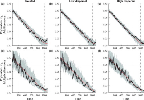
Table 1. Parameter values for numerical simulations.

Parameter	Symbol	Value (per unit time)
Fraction of population that disperse (high level)	$m_{\mathrm{h}}$	0.2
Fraction of population that disperse (low level)	$m_{\mathrm{l}}$	0.01
Additive noise level	${\sigma }_a$	0.001
Mechanistic (multiplicative) noise level	${\sigma }_{\mu }$	0.05
Initial intrinsic growth rate (homogeneous model)	r	0.1
Intrinsic growth rate (strong source patch 1)	$r_1$	0.1
Intrinsic growth rate (weak source patch 1)	$r_1$	0.02
Initial intrinsic growth rate (in deteriorating patch 2)${}^{\mathrm{a}}$	$r_2$	0.1
Rate of change of intrinsic growth rate (deteriorating patch)	$r_0$	${10}^{-5}$
Estimated time to extinction predicted by model (6(6) $\begin{array}{rl}\frac{\mathrm{d}{x}_1}{\mathrm{d}t}& =r_1\left(t\right)x_1-x_1^2-m{x}_1+m{x}_2,\\ \frac{\mathrm{d}{x}_2}{\mathrm{d}t}& =r_2\left(t\right)x_2-x_2^2-m{x}_2+m{x}_1,\end{array}$(6) )	$t^{\ast }$	1000
Initial population $x_i$ value (homogeneous system)	$x_i\left(0\right)$	0.1
Initial population $x_1$ value (strong source patch)	$x_1\left(0\right)$	0.1
Initial population $x_1$ value (weak source patch)	$x_1\left(0\right)$	0.02
Initial population $x_2$ value (deteriorating patch)	$x_2\left(0\right)$	0.1

^aWe explore the effects of spatial heterogeneity by assuming that conditions deteriorate in the second patch only.

3. Leading indicators of population extinction

To anticipate subpopulation extinction from time series of each subpopulation, we seek to quantify the behaviour of subpopulation fluctuations through temporal leading indicator statistics. Here, we will show that three leading indicator statistics change systematically as extinction is approached, as a direct result of increases in the return rate of the system to the steady state. The steady state here is taken to be the mean of the quasi-stationary population distribution. Consequently, we let $r_i\left(t\right)=r_i$ in models (9(9) $\begin{array}{rl}\mathrm{d}{x}_1& =\left(r_1\right(t)x_1-x_1^2-m{x}_1+m{x}_2)\mathrm{d}t+{\sigma }_a\mathrm{d}{W}_1,\\ \mathrm{d}{x}_2& =\left(r_2\right(t)x_2-x_2^2-m{x}_2+m{x}_1))\mathrm{d}t+{\sigma }_a\mathrm{d}{W}_2.\end{array}$(9) ) and (12(12) $\begin{array}{rl}\mathrm{d}{x}_1& =\left(r_1\right(t)x_1-x_1^2-m{x}_1+m{x}_2)\mathrm{d}t+{\sigma }_{\mu }{x}_1\mathrm{d}{W}_1,\\ \mathrm{d}{x}_2& =\left(r_2\right(t)x_2-x_2^2-m{x}_2+m{x}_1))\mathrm{d}t+{\sigma }_{\mu }{x}_2\mathrm{d}{W}_2.\end{array}$(12) ) and quantify the behaviour of fluctuations near the positive steady state $(x_1^{\ast },x_2^{\ast })$ of model (1(1) $\begin{array}{rl}\frac{\mathrm{d}{x}_1}{\mathrm{d}t}& =r_1{x}_1-x_1^2-m{x}_1+m{x}_2,\\ \frac{\mathrm{d}{x}_2}{\mathrm{d}t}& =r_2{x}_2-x_2^2-m{x}_2+m{x}_1,\end{array}$(1) ). Of course, the fast-slow models assume the mean is evolving slowly through time, but the steady state is a useful approximation for the mean of the fast-slow models provided that the intrinsic growth rate in each patch changes sufficiently slowly. Recall that by Fenichel's Theorem, since $0<r_0<<1$, the dynamics of the fast-slow system approach those of the system where $r_i$ is constant.

To derive summary statistics for fluctuations about the positive steady state, we first note that we can express systems (9(9) $\begin{array}{rl}\mathrm{d}{x}_1& =\left(r_1\right(t)x_1-x_1^2-m{x}_1+m{x}_2)\mathrm{d}t+{\sigma }_a\mathrm{d}{W}_1,\\ \mathrm{d}{x}_2& =\left(r_2\right(t)x_2-x_2^2-m{x}_2+m{x}_1))\mathrm{d}t+{\sigma }_a\mathrm{d}{W}_2.\end{array}$(9) ) and (12(12) $\begin{array}{rl}\mathrm{d}{x}_1& =\left(r_1\right(t)x_1-x_1^2-m{x}_1+m{x}_2)\mathrm{d}t+{\sigma }_{\mu }{x}_1\mathrm{d}{W}_1,\\ \mathrm{d}{x}_2& =\left(r_2\right(t)x_2-x_2^2-m{x}_2+m{x}_1))\mathrm{d}t+{\sigma }_{\mu }{x}_2\mathrm{d}{W}_2.\end{array}$(12) ) as follows, (13) $\mathrm{d}x\left(t\right)=f\left(x\right(t),t)\mathrm{d}t+\sqrt{D\left(x\right(t),t)}\mathrm{d}W\left(t\right),$(13) where $x\left(t\right)=(x_1,x_2)$, the terms of the mean vector $f\left(x\right(t),t)$ are $f_i\left(x\right(t),t)=(r_i{x}_i-x_i^2-m{x}_i+m{x}_j)$ and the entries of the variance–covariance matrix $D\left(x\right(t),t)$ are $D_{ii}\left(x\right(t),t)={\sigma }_a^2$ for additive noise and are $D_{ii}\left(x\right(t),t)={\sigma }_{\mu }^2{x}_i^2$ for multiplicative noise ($D_{ij}\left(x\right(t),t)=0$ in both models since the subpopulations do not covary with each other). The probability distribution $P\left(x\right(t),t)$ of the solutions of system (13(13) $\mathrm{d}x\left(t\right)=f\left(x\right(t),t)\mathrm{d}t+\sqrt{D\left(x\right(t),t)}\mathrm{d}W\left(t\right),$(13) ) satisfies the forward Kolmogorov equation [2], (14) $\begin{array}{r}\frac{\mathrm{\partial }P\left(x\right(t),t)}{\mathrm{\partial }t}=-\sum _{i=1}^2\frac{\mathrm{\partial }}{\mathrm{\partial }{x}_i}\left(f_i\right(x\left(t\right),t\left)P\right(x\left(t\right),t\left)\right)+\frac{1}{2}\sum _{i=1}^2\sum _{j=1}^2\frac{\mathrm{\partial }}{\mathrm{\partial }{x}_i{x}_j}\left(D_{ij}\right(x\left(t\right),t\left)P\right(x\left(t\right),t\left)\right).\end{array}$(14)

3.1. Linearization of the model

To quantify the behaviour of fluctuations near the positive steady state, we Taylor expand the terms in the mean vector and variance–covariance matrix about $(x_1^{\ast },x_2^{\ast })$, retaining leading order terms, $\begin{array}{rl}{f}_i(x_1,x_2,t)& \approx f_i(x_1^{\ast },x_2^{\ast },t)+\frac{\mathrm{\partial }{f}_i(x_1^{\ast },x_2^{\ast },t)}{\mathrm{\partial }{x}_1}{z}_1+\frac{\mathrm{\partial }{f}_i(x_1^{\ast },x_2^{\ast },t)}{\mathrm{\partial }{x}_2}{z}_2+\cdots \\ & \approx 0+\sum _{j=1}^2{a}_{ij}{z}_j\cdots ,\end{array}$ where $a_{ij}$ denote the partial derivatives of $f_i$ and $z_i=x_i-x_i^{\ast }$ denote perturbations from the steady state. Similarly, $D_{ij}(x_1,x_2,t)\approx D_{ij}(x_1^{\ast },x_2^{\ast },t)+\cdots .$ The entries $a_{ij}$ of the Jacobian matrix are given by $a_{ii}=r_i-2x_i^{\ast }-m$, $a_{ij}=m$, $i\ne j$, and the terms of the variance–covariance matrix are $D_{ii}={\sigma }_a$ for additive noise and $D_{ii}={\sigma }_{\mu }{x}_i^{\ast }$ for multiplicative noise. The joint probability distribution of fluctuations $z\left(t\right)=(z_1,z_2)$ from the steady state satisfies (15) $\frac{\mathrm{\partial \Pi }\left(z\right(t),t)}{\mathrm{\partial }t}=-\sum _{i=1}^2\frac{\mathrm{\partial }}{\mathrm{\partial }{z}_i}\mathrm{\Pi }\left(z\right(t),t)\left(\sum _{j=1}^2{a}_{ij}{z}_i\right)+\frac{1}{2}\sum _{i=1}^2\sum _{j=1}^2\frac{\mathrm{\partial }}{\mathrm{\partial }{z}_i{z}_j}\left(D_{ij}\mathrm{\Pi }\right(z\left(t\right),t\left)\right).$(15) Solutions of the following system of stochastic differential equations, (16) $\begin{array}{rl}\mathrm{d}{z}_1& =(a_{11}{z}_1+a_{12}{z}_2)\mathrm{d}t+\sqrt{D_{11}}\mathrm{d}{W}_1\\ \mathrm{d}{z}_2& =(a_{21}{z}_1+a_{22}{z}_2)\mathrm{d}t+\sqrt{D_{22}}\mathrm{d}{W}_2\end{array}$(16) have the same probability distribution $\mathrm{\Pi }\left(z\right(t),t)$ [3].

3.2. Derivation of the spectral density

To derive leading indicators of extinction, we first derive the spectral density of the fluctuating subpopulation in each patch. The spectral density is a function that delineates how the amplitudes of each component of the fluctuations in each subpopulation are distributed with respect to angular frequency. It can be obtained through the technique of Fourier transforms. Here we briefly outline the Fourier transformation method.

We note that any continuous function $z\left(t\right)$ defined in the time interval $-T/2\le t\le T/2$ may be written in terms of its Fourier transform $\tilde{z}\left(\omega \right)$, (17) $z\left(t\right)=\frac{1}{2\pi }{\int }_{-\mathrm{\infty }}^{\mathrm{\infty }}\tilde{z}\left(\omega \right)\exp \left(i\omega t\right)\mathrm{d}\omega ,$(17) where ω denotes angular frequency. Roughly, Equation (17(17) $z\left(t\right)=\frac{1}{2\pi }{\int }_{-\mathrm{\infty }}^{\mathrm{\infty }}\tilde{z}\left(\omega \right)\exp \left(i\omega t\right)\mathrm{d}\omega ,$(17) ) describes a superposition of amplitudes of all the angular frequency components of the signal $z\left(t\right)$. Consequently, Fourier transformation of a time-varying function or signal conveniently describes the underlying frequencies that comprise it [33]. The Fourier transform of $z\left(t\right)$ is given by (18) $\tilde{z}\left(\omega \right)={\int }_{-T/2}^{T/2}z\left(t\right)\exp (-i\omega t)\mathrm{d}t.$(18) We rewrite system (16(16) $\begin{array}{rl}\mathrm{d}{z}_1& =(a_{11}{z}_1+a_{12}{z}_2)\mathrm{d}t+\sqrt{D_{11}}\mathrm{d}{W}_1\\ \mathrm{d}{z}_2& =(a_{21}{z}_1+a_{22}{z}_2)\mathrm{d}t+\sqrt{D_{22}}\mathrm{d}{W}_2\end{array}$(16) ) in a convenient form for Fourier transformation, (19) $\begin{array}{rl}\frac{\mathrm{d}{z}_1}{\mathrm{d}t}& =a_{11}{z}_1\left(t\right)+a_{12}{z}_2\left(t\right)+\sqrt{D_{11}}{\mathrm{\Gamma }}_1\left(t\right),\\ \frac{\mathrm{d}{z}_2}{\mathrm{d}t}& =a_{21}{z}_1\left(t\right)+a_{22}{z}_2\left(t\right)+\sqrt{D_{22}}{\mathrm{\Gamma }}_2\left(t\right),\end{array}$(19) where ${\mathrm{\Gamma }}_1\left(t\right)$ and ${\mathrm{\Gamma }}_2\left(t\right)$ represent white noise processes associated with the covariance matrix $\left\{D_{ij}\right\}$. Fourier transformation of system (19(19) $\begin{array}{rl}\frac{\mathrm{d}{z}_1}{\mathrm{d}t}& =a_{11}{z}_1\left(t\right)+a_{12}{z}_2\left(t\right)+\sqrt{D_{11}}{\mathrm{\Gamma }}_1\left(t\right),\\ \frac{\mathrm{d}{z}_2}{\mathrm{d}t}& =a_{21}{z}_1\left(t\right)+a_{22}{z}_2\left(t\right)+\sqrt{D_{22}}{\mathrm{\Gamma }}_2\left(t\right),\end{array}$(19) ) yields, (20) $\begin{array}{rl}i\omega \widetilde{z_1}\left(\omega \right)& =a_{11}\widetilde{z_1}\left(\omega \right)+a_{12}\widetilde{z_2}\left(\omega \right)+\sqrt{D_{11}}\widetilde{{\mathrm{\Gamma }}_1}\left(\omega \right),\\ i\omega \widetilde{z_2}\left(\omega \right)& =a_{21}\widetilde{z_1}\left(\omega \right)+a_{22}\widetilde{z_2}\left(\omega \right)+\sqrt{D_{22}}\widetilde{{\mathrm{\Gamma }}_2}\left(\omega \right),\end{array}$(20) where $\widetilde{z_1}\left(\omega \right)$, $\widetilde{z_2}\left(\omega \right)$, $\widetilde{{\mathrm{\Gamma }}_1}\left(\omega \right)$ and $\widetilde{{\mathrm{\Gamma }}_2}\left(\omega \right)$ are the Fourier transforms of the functions $z_1\left(t\right)$, $z_2\left(t\right)$, ${\mathrm{\Gamma }}_1\left(t\right)$ and ${\mathrm{\Gamma }}_2\left(t\right)$, respectively. After some algebra, we obtain an expression from Equation (20(20) $\begin{array}{rl}i\omega \widetilde{z_1}\left(\omega \right)& =a_{11}\widetilde{z_1}\left(\omega \right)+a_{12}\widetilde{z_2}\left(\omega \right)+\sqrt{D_{11}}\widetilde{{\mathrm{\Gamma }}_1}\left(\omega \right),\\ i\omega \widetilde{z_2}\left(\omega \right)& =a_{21}\widetilde{z_1}\left(\omega \right)+a_{22}\widetilde{z_2}\left(\omega \right)+\sqrt{D_{22}}\widetilde{{\mathrm{\Gamma }}_2}\left(\omega \right),\end{array}$(20) ) for the Fourier transform $\widetilde{z_1}\left(\omega \right)$, (21) $\widetilde{z_1}\left(\omega \right)=\frac{(a_{22}-i\omega )\sqrt{D_{11}}{\mathrm{\Gamma }}_1\left(\omega \right)}{d-{\omega }^2-iT\omega }-\frac{a_{12}\sqrt{D_{22}}{\mathrm{\Gamma }}_2\left(\omega \right)}{d-{\omega }^2-iT\omega },$(21) where T and d are the trace and determinant of the Jacobian matrix $\left\{a_{ij}\right\}$, respectively. Using Equation (21(21) $\widetilde{z_1}\left(\omega \right)=\frac{(a_{22}-i\omega )\sqrt{D_{11}}{\mathrm{\Gamma }}_1\left(\omega \right)}{d-{\omega }^2-iT\omega }-\frac{a_{12}\sqrt{D_{22}}{\mathrm{\Gamma }}_2\left(\omega \right)}{d-{\omega }^2-iT\omega },$(21) ) we can establish the spectral density of the fluctuations (see Appendix for the formal definition and details of the calculation), which we denote by (22) $S_1\left(\omega \right)=\frac{D_{11}{a}_{22}^2+D_{22}{a}_{12}^2+D_{11}{\omega }^2}{({\omega }^2-d{)}^2+T^2{\omega }^2}.$(22) Through similar calculations, we obtain the spectral density of fluctuations of the subpopulation in patch 2, (23) $S_2\left(\omega \right)=\frac{D_{22}{a}_{11}^2+D_{11}{a}_{21}^2+D_{22}{\omega }^2}{({\omega }^2-d{)}^2+T^2{\omega }^2}.$(23) The spectral density function describes the expectation of the square of the modulus of the Fourier-transformed signal $z\left(t\right)$ averaged over all time, and it is a measure of how the amplitudes of all the angular frequency components of a stationary process $z\left(t\right)$ are distributed with frequency. Equations (22(22) $S_1\left(\omega \right)=\frac{D_{11}{a}_{22}^2+D_{22}{a}_{12}^2+D_{11}{\omega }^2}{({\omega }^2-d{)}^2+T^2{\omega }^2}.$(22) ) and (23(23) $S_2\left(\omega \right)=\frac{D_{22}{a}_{11}^2+D_{11}{a}_{21}^2+D_{22}{\omega }^2}{({\omega }^2-d{)}^2+T^2{\omega }^2}.$(23) ) are functions of environmental variability, intrinsic growth rate in each patch and coupling between the patches. Consequently, all of these quantities contribute to the size of subpopulation fluctuations in each patch.

Various temporal leading indicator statistics can be derived from the spectral density $S_i\left(\omega \right)$. The variance, lag-1 autocovariance function, lag-1 autocorrelation function and coefficient of variation of the fluctuations around the steady state $(x_1^{\ast },x_2^{\ast })$ may be obtained using Equations (22(22) $S_1\left(\omega \right)=\frac{D_{11}{a}_{22}^2+D_{22}{a}_{12}^2+D_{11}{\omega }^2}{({\omega }^2-d{)}^2+T^2{\omega }^2}.$(22) ) and (23(23) $S_2\left(\omega \right)=\frac{D_{22}{a}_{11}^2+D_{11}{a}_{21}^2+D_{22}{\omega }^2}{({\omega }^2-d{)}^2+T^2{\omega }^2}.$(23) ) through integration, (e.g. as in [33, 34]). Variance and coefficient of variation are measures of the size of fluctuations as extinction is approached. The lag-τ autocovariance function of a signal $z\left(t\right)$ is $\underset{T\to \mathrm{\infty }}{lim}\frac{1}{T}{\int }_0^{\mathrm{T}}\left(z\right(t)-z^{\ast })\left(z\right(t+\tau )-z^{\ast })\mathrm{d}t,$ where $z^{\ast }$ denotes the long-term average value of the signal. The lag-τ autocovariance and autocorrelation functions quantify the degree of memory in the system. Essentially, points in the time series of residuals $z_i\left(t\right)$ and $z_i(t+\tau )$ become increasingly correlated as a bifurcation is approached, due to critical slowing down of the system.

To obtain the variance of the fluctuations of subpopulation i in each patch, we integrate the spectral density over all frequencies, taking advantage of the evenness of $S_i\left(\omega \right)$ [33], (24) $\frac{1}{2\pi }{\int }_{-\mathrm{\infty }}^{\mathrm{\infty }}{S}_i\left(\omega \right)\mathrm{d}\omega =\frac{1}{\pi }{\int }_0^{\mathrm{\infty }}{S}_i\left(\omega \right)\mathrm{d}\omega .$(24) To obtain the lag-τ autocovariance function of $x_i$, we calculate [33] (25) $\frac{1}{2\pi }{\int }_{-\mathrm{\infty }}^{\mathrm{\infty }}{S}_i\left(\omega \right)\cos \left(\omega \tau \right)\mathrm{d}\omega =\frac{1}{\pi }{\int }_0^{\mathrm{\infty }}{S}_i\left(\omega \right)\cos \left(\omega \tau \right)\mathrm{d}\omega .$(25) Dividing Equation (25(25) $\frac{1}{2\pi }{\int }_{-\mathrm{\infty }}^{\mathrm{\infty }}{S}_i\left(\omega \right)\cos \left(\omega \tau \right)\mathrm{d}\omega =\frac{1}{\pi }{\int }_0^{\mathrm{\infty }}{S}_i\left(\omega \right)\cos \left(\omega \tau \right)\mathrm{d}\omega .$(25) ) by the variance yields the lag-τ autocorrelation function for subpopulation i. The coefficient of variation can be obtained from dividing the square root of the subpopulation variance by the subpopulation mean. All of these statistics can be obtained through numerical integration, but in the homogeneous case, it is possible to derive simple expressions for variance, lag-1 autocovariance, lag-1 autocorrelation and coefficient of variation, which yield analytical insight into how these statistics signal the onset of critical slowing down in the homogeneous spatial system prior to the bifurcation.

3.3. Derivations of leading indicators from the spatially homogeneous model

Here, we derive analytical expressions for the variance, coefficient of variation, lag-1 autocovariance function and lag-1 autocorrelation function for the spatially homogeneous model with r>0 and m>0. For the spatially homogeneous model, $a_{11}=a_{22}=-r-m$ and $a_{12}=a_{21}=m$. If noise is additive in nature, the spectral density of the fluctuations of the subpopulations in each patch i is given by (26) $S_i\left(\omega \right)=\frac{{\sigma }_a^2(-r-m{)}^2+{\sigma }_a^2{m}^2+{\sigma }_a^2{\omega }^2}{({\omega }^2-((-r-m{)}^2-m^2){)}^2+(-2r-2m{)}^2{\omega }^2}.$(26) To obtain the variance of the fluctuations, we integrate the spectral density over all frequencies, $\frac{1}{2\pi }{\int }_{-\mathrm{\infty }}^{\mathrm{\infty }}{S}_i\left(\omega \right)\mathrm{d}\omega =\frac{1}{\pi }{\int }_0^{\mathrm{\infty }}{S}_i\left(\omega \right)\mathrm{d}\omega .$ Evaluating this expression yields (27) $v_a\left(r\right)=\frac{(m+r){\sigma }_a^2}{2r(2m+r)}.$(27) To obtain the autocovariance function, we calculate (28) $\frac{1}{2\pi }{\int }_{-\mathrm{\infty }}^{\mathrm{\infty }}{S}_i\left(\omega \right)\cos \left(\omega \tau \right)\mathrm{d}\omega =\frac{1}{\pi }{\int }_0^{\mathrm{\infty }}{S}_i\left(\omega \right)\cos \left(\omega \tau \right)\mathrm{d}\omega ,$(28) taking advantage of the evenness of $S_i\left(\omega \right)$. Since we are interested in the lag-1 autocovariance function, we set the time lag τ to unity. Integrating expression (28(28) $\frac{1}{2\pi }{\int }_{-\mathrm{\infty }}^{\mathrm{\infty }}{S}_i\left(\omega \right)\cos \left(\omega \tau \right)\mathrm{d}\omega =\frac{1}{\pi }{\int }_0^{\mathrm{\infty }}{S}_i\left(\omega \right)\cos \left(\omega \tau \right)\mathrm{d}\omega ,$(28) ) with $\tau =1$ gives (29) $a_a\left(r\right)=\frac{{\sigma }_a^2\exp (-2m-r)}{4(2m+r)}+\frac{{\sigma }^2\exp (-r)}{4r}.$(29) Dividing this expression by the variance yields the lag-1 autocorrelation function, (30) ${\mathrm{acf}}_a\left(r\right)=\frac{1}{2(m+r)}(r\exp (-2m-r)+(2m+r)\exp (-r\left)\right).$(30) We note that the variance and lag-1 autocorrelation functions can be expressed in terms of the eigenvalues ${\lambda }_i$, i=1,2 of the spatially homogeneous system, (31) $\begin{array}{rl}{v}_a\left(r\right)& =\frac{{\sigma }_a^2}{4}\frac{|{\lambda }_1|+|{\lambda }_2|}{|{\lambda }_1||{\lambda }_2|},\end{array}$(31) (32) $\begin{array}{rl}{\mathrm{acf}}_1\left(r\right)& =\frac{1}{|{\lambda }_1|+|{\lambda }_2|}(|{\lambda }_1|\exp (-|{\lambda }_2|)+|{\lambda }_2|\exp (-|{\lambda }_1|\left)\right).\end{array}$(32) The return rate to the steady state, which is determined by the magnitude of the eigenvalues, governs the behaviour of the summary statistics.

Alternatively, if noise is multiplicative, the spectral density of the fluctuations is (33) $S_i\left(\omega \right)=\frac{\left({\sigma }_{\mu }r{)}^2\right(-r-m{)}^2+({\sigma }_{\mu }r{)}^2{m}^2+({\sigma }_{\mu }r{)}^2{\omega }^2}{({\omega }^2-((-r-m{)}^2-m^2){)}^2+(-2r-2m{)}^2{\omega }^2}.$(33) Repeating the analysis for the multiplicative noise case yields the following expressions for the variance, lag-1 autocovariance and lag-1 autocorrelation functions, (34) $\begin{array}{rl}{v}_{\mu }(r,m)& =\frac{r(m+r){\sigma }_{\mu }^2}{2(2m+r)}\end{array}$(34) (35) $\begin{array}{rl}{a}_{\mu }(r,m)& =\frac{{\sigma }_{\mu }^2{r}^2\exp (-2m-r)}{4(2m+r)}+\frac{r(2m+r){\sigma }_{\mu }^2\exp (-r)}{4(2m+r)}\end{array}$(35) (36) $\begin{array}{rl}{\mathrm{acf}}_1\left(r\right)& =\frac{1}{2(m+r)}(r\exp (-2m-r)+(2m+r)\exp (-r\left)\right).\end{array}$(36) Notice that the lag-1 autocorrelation functions are equal for both noise types, and are determined entirely by the deterministic dynamics. Additionally, the variance can be expressed in terms of the magnitudes of the eigenvalues ${\lambda }_1=-r$ and ${\lambda }_2=-r-2m$, (37) $v_{\mu }(r,m)=\frac{{\sigma }_{\mu }^2}{4}(|{\lambda }_1|+|{\lambda }_2|)\frac{|{\lambda }_1|}{|{\lambda }_2|}.$(37)

To obtain the coefficient of variation statistic for each patch, a measure of variability standardized by the mean, we simply divide the standard deviation (square root of the fluctuation variance) by the subpopulation mean r in each patch, (38) $\begin{array}{rl}{\mathrm{CV}}_a(r,m)& =\frac{\sqrt{m+r}{\sigma }_a}{r\sqrt{2r(2m+r)}},\end{array}$(38) (39) $\begin{array}{rl}{\mathrm{CV}}_{\mu }(r,m)& =\frac{\sqrt{m+r}{\sigma }_{\mu }}{\sqrt{2r(2m+r)}}.\end{array}$(39) In summary, measures of variability depend on the strength of noise, and moreover, the type of noise (additive vs. multiplicative) influences their functional forms. It is evident that all of these indicators are continuous functions of the intrinsic growth rate r and the strength of coupling m. All of the leading indicator functions exist for r in $(0,\mathrm{\infty })$ and are defined for m in $(0,\mathrm{\infty })$.

3.4. Predicted behaviour of leading indicators derived from the spatially homogeneous model

Finally, we are interested in the qualitative behaviour of the leading indicators as patch quality deteriorates, that is, the intrinsic growth rate r of each subpopulation approaches zero from the right, for all r in $(0,\mathrm{\infty })$. Taking the limit of each expression as $r\to 0^{+}$ yields, (40) $\begin{array}{rl}\underset{r\to 0^{+}}{lim}{v}_a(r,m)& =\underset{r\to 0^{+}}{lim}\frac{(m+r){\sigma }_a^2}{2r(2m+r)}=+\mathrm{\infty },\end{array}$(40) (41) $\begin{array}{rl}\underset{r\to 0^{+}}{lim}{v}_{\mu }(r,m)& =\underset{r\to 0^{+}}{lim}\frac{r(m+r){\sigma }_{\mu }^2}{2(2m+r)}=0,\end{array}$(41) (42) $\begin{array}{rl}\underset{r\to 0^{+}}{lim}{\mathrm{CV}}_a(r,m)& =\underset{r\to 0^{+}}{lim}\frac{\sqrt{m+r}{\sigma }_a}{r\sqrt{2r(2m+r)}}=+\mathrm{\infty },\end{array}$(42) (43) $\begin{array}{rl}\underset{r\to 0^{+}}{lim}{\mathrm{CV}}_{\mu }(r,m)& =\underset{r\to 0^{+}}{lim}\frac{\sqrt{m+r}{\sigma }_{\mu }}{\sqrt{2r(2m+r)}}=+\mathrm{\infty },\end{array}$(43) (44) $\begin{array}{rl}\underset{r\to 0^{+}}{lim}{\mathrm{acf}}_1(r,m)& =\underset{r\to 0^{+}}{lim}\left\{\frac{1}{2(m+r)}\right(r\exp (-2m-r)+(2m+r)\exp (-r)\left)\right\}=1.\end{array}$(44) To understand how the statistics change as extinction is approached due to changes in intrinsic dynamics, we calculate the first derivative of each statistic with respect to r (Table 2). By taking the first derivative of each function with respect to r, provided m and r are strictly positive, $v_a(r,m)$, ${\mathrm{CV}}_a(r,m)$, ${\mathrm{CV}}_{\mu }(r,m)$ and ${\mathrm{acf}}_1(r,m)$ are strictly decreasing functions of r, and consequently, all of these functions increase monotonically as r approaches zero from the right (Table 2). On the other hand, $v_{\mu }\left(r\right)$ is a strictly increasing function of r, and thus decreases monotonically as r tends to zero. Therefore, we predict strictly increasing trends in lag-1 autocorrelation and coefficient of variation, as extinction is approached in each patch, and strictly increasing variance if noise is additive, and strictly decreasing variance if noise is multiplicative.

Table 2. First derivatives of each statistic, assuming m>0, r>0 and $\sigma >0$.

Statistic $h(r,m)$	${\displaystyle \frac{\mathrm{\partial }}{\mathrm{\partial }r}}h(r,m)$	${\displaystyle \frac{\mathrm{\partial }}{\mathrm{\partial }m}}h(r,m)$
$v_a(r,m)$	$-{\displaystyle \frac{(2m^2+2mr+r^2){\sigma }_a^2}{2r^2(2m+r{)}^2}}$	$-{\displaystyle \frac{{\sigma }_a^2}{2(2m+r{)}^2}}$
$v_{\mu }(r,m)$	${\displaystyle \frac{(2m^2+4mr+r^2){\sigma }_{\mu }^2}{2(2m+r{)}^2}}$	$-{\displaystyle \frac{r^2{\sigma }_{\mu }^2}{2(2m+r{)}^2}}$
${\mathrm{CV}}_a(r,m)$	$-{\displaystyle \frac{(6m^2+8mr+3r^2){\sigma }_a}{2\sqrt{2}{r}^{5/2}(2m+r{)}^{3/2}(m+r{)}^{1/2}}}$	$-{\displaystyle \frac{r{\left({\displaystyle \frac{(m+r){\sigma }_a^2}{r(2m+r)}}\right)}^{3/2}}{2\sqrt{2}(m+r{)}^2{\sigma }_a^2}}$
${\mathrm{CV}}_{\mu }(r,m)$	$-{\displaystyle \frac{(m+r)(2m^2+2mr+r^2){\sigma }_{\mu }}{2\sqrt{2}(2m+r{)}^{3/2}(r(m+r){)}^{3/2})}}$	$-{\displaystyle \frac{r{\sigma }_{\mu }}{2\sqrt{2}(2m+r{)}^{3/2}\sqrt{\left(r\right(m+r)}}}$
${\mathrm{acf}}_1(r,m)$	$\begin{array}{rl}& \frac{1}{(m+r{)}^2}\left(\right(m+r{)}^2\cosh \left(m\right)\\ & +m(1+m+r)\sinh \left(m\right))\\ & \times (-\exp (-(m+r))\end{array}$	${\displaystyle \frac{\exp (-2m-r)(-1+\exp (2m)-2m-2r)r}{2(m+r{)}^2}}$

To understand the effect of coupling on the behaviour of the temporal leading indicators, we examine the functions as m approaches zero from the right, and as m approaches positive infinity. As the degree of coupling decreases, the populations in each patch behave like isolated subpopulations, whereas when coupling increases, and the subpopulations become more well-mixed, the metapopulation behaves like one large patch.

As m decreases to zero from the right, the limit of each statistic approaches the expression for the statistic in the absence of dispersal [33], (45) $\begin{array}{rl}\underset{m\to 0^{+}}{lim}{v}_a(r,m)& =\underset{m\to 0^{+}}{lim}\frac{(m+r){\sigma }_a^2}{2r(2m+r)}=\frac{{\sigma }_a^2}{2r},\end{array}$(45) (46) $\begin{array}{rl}\underset{m\to 0^{+}}{lim}{v}_{\mu }(r,m)& =\underset{m\to 0^{+}}{lim}\frac{r(m+r){\sigma }_{\mu }^2}{2(2m+r)}=\frac{r{\sigma }_{\mu }^2}{2},\end{array}$(46) (47) $\begin{array}{rl}\underset{m\to 0^{+}}{lim}{\mathrm{CV}}_a(r,m)& =\underset{m\to 0^{+}}{lim}\frac{\sqrt{m+r}{\sigma }_a}{r\sqrt{2r(2m+r)}}=\frac{{\sigma }_a}{r\sqrt{2r}},\end{array}$(47) (48) $\begin{array}{rl}\underset{m\to 0^{+}}{lim}{\mathrm{CV}}_{\mu }(r,m)& =\underset{m\to 0^{+}}{lim}\frac{\sqrt{m+r}{\sigma }_{\mu }}{\sqrt{2r(2m+r)}}=\frac{{\sigma }_{\mu }}{\sqrt{2r}},\end{array}$(48) (49) $\begin{array}{rl}\underset{m\to 0^{+}}{lim}{\mathrm{acf}}_1(r,m)& =\underset{m\to 0^{+}}{lim}\left\{\frac{1}{2(m+r)}\right(r\exp (-2m-r)+(2m+r)\exp (-r)\left)\right\}\\ & =\exp (-r).\end{array}$(49) Consequently, the summary statistics capture the behaviour of the metapopulation as being similar to isolated subpopulations. If coupling increases to infinity, the limits are (50) $\begin{array}{rl}\underset{m\to \mathrm{\infty }}{lim}{v}_a(r,m)& =\underset{m\to \mathrm{\infty }}{lim}\frac{(m+r){\sigma }_a^2}{2r(2m+r)}=\frac{{\sigma }_a^2}{4r},\end{array}$(50) (51) $\begin{array}{rl}\underset{m\to \mathrm{\infty }}{lim}{v}_{\mu }(r,m)& =\underset{m\to \mathrm{\infty }}{lim}\frac{r(m+r){\sigma }_{\mu }^2}{2(2m+r)}=\frac{r{\sigma }_{\mu }^2}{4},\end{array}$(51) (52) $\begin{array}{rl}\underset{m\to \mathrm{\infty }}{lim}{\mathrm{CV}}_a(r,m)& =\underset{m\to \mathrm{\infty }}{lim}\frac{\sqrt{m+r}{\sigma }_a}{r\sqrt{2r(2m+r)}}=\frac{{\sigma }_a}{2r\sqrt{r}},\end{array}$(52) (53) $\begin{array}{rl}\underset{m\to \mathrm{\infty }}{lim}{\mathrm{CV}}_{\mu }(r,m)& =\underset{m\to \mathrm{\infty }}{lim}\frac{\sqrt{m+r}{\sigma }_{\mu }}{\sqrt{2r(2m+r)}}=\frac{{\sigma }_{\mu }}{2\sqrt{r}},\end{array}$(53) (54) $\begin{array}{rl}\underset{m\to \mathrm{\infty }}{lim}{\mathrm{acf}}_1(r,m)& =\underset{m\to \mathrm{\infty }}{lim}\left\{\frac{1}{2(m+r)}\right(r\exp (-2m-r)+(2m+r)\exp (-r)\left)\right\}\\ & =\exp (-r).\end{array}$(54) Increasing the level of migration between patches muffles the temporal signals that measure variability. As m approaches $+\mathrm{\infty }$, the limit of the variance approaches 1/2 of the limit of the variance in the absence of dispersal, in both additive and multiplicative cases. In a very well-mixed metapopulation, temporal variance in each patch will be muffled relative to isolated patches. Similarly, as m approaches $+\mathrm{\infty }$, the limit of the coefficient of variation approaches $1/\sqrt{2}$ of its limit in the absence of coupling, in both noise regimes. Table 2 shows that the derivative of each function monotonically decreases with m, provided m>0, r>0 and $\sigma >0$.

Notice that the limit of the lag-1 autocorrelation function approaches $\exp (-r)$ as m approaches 0 and $+\mathrm{\infty }$. The first derivative of ${\mathrm{acf}}_1(m,r)$ with respect to m is, (55) $\frac{\mathrm{\partial }}{\mathrm{\partial }m}{\mathrm{acf}}_1(r,m)=\frac{\exp (-2m-r)(-1+\exp (2m)-2m-2r)r}{2(m+r{)}^2}.$(55) Provided m and r are strictly positive, a critical point of ${\mathrm{acf}}_1(m,r)$ exists at (56) $m_c=-\frac{1}{2}-r-\frac{1}{2}\mathrm{ProductLog}[-1,-\exp ((-1-2r)\left)\right].$(56) The second derivative test indicates that a local minimum of ${\mathrm{acf}}_1(m,r)$ occurs at $m_c$. Differentiating expression (55(55) $\frac{\mathrm{\partial }}{\mathrm{\partial }m}{\mathrm{acf}}_1(r,m)=\frac{\exp (-2m-r)(-1+\exp (2m)-2m-2r)r}{2(m+r{)}^2}.$(55) ) with respect to m and evaluating the resulting function at $m_c$ yields (57) $\begin{array}{rl}& \frac{{\mathrm{\partial }}^2{\mathrm{acf}}_1(r,m_c)}{{\mathrm{\partial }}^{2}m}\\ & =\frac{4r\exp (-r)}{\mathrm{ProductLog}[-1,-\exp ((-1-2r)]+\mathrm{ProductLog}[-1,-\exp \left(\right(-1-2r){]}^2}.\end{array}$(57) The second derivative is always positive at $m_c$, since $\exp (-r)>0$, r>0, and the denominator of expression (57(57) $\begin{array}{rl}& \frac{{\mathrm{\partial }}^2{\mathrm{acf}}_1(r,m_c)}{{\mathrm{\partial }}^{2}m}\\ & =\frac{4r\exp (-r)}{\mathrm{ProductLog}[-1,-\exp ((-1-2r)]+\mathrm{ProductLog}[-1,-\exp \left(\right(-1-2r){]}^2}.\end{array}$(57) ) is strictly positive since the square term dominates.

Consequently, when dispersal is low in the spatially homogeneous system, points $x_i\left(t\right)$ and $x_i(t+1)$ in a stationary time series are highly correlated. As dispersal increases, temporal correlation between $x_i\left(t\right)$ and $x_i(t+1)$ decreases, due to mixing between subpopulations. For $m>m_c$, however, points become increasingly autocorrelated because migration is high enough between patches to cause the metapopulation to behave as one patch. In sum, $x_i\left(t\right)$ and $x_i(t+1)$ are least correlated at intermediate levels of coupling. For intermediate levels of dispersal, we expect the lag-1 autocorrelation to be decreased relative to that in isolated patches, but if coupling is sufficiently high, lag-1 autocorrelation approaches that of a single patch.

3.5. Numerical predictions for the summary statistics for the spatially homogeneous system

Evaluating the summary statistics numerically about the mean $(x_1^{\ast },x_2^{\ast })=(r,r)$ confirms the theoretical predictions in Section 3.4. As the growth rate r approaches zero from the right in each patch, trends in the leading indicators change as predicted by the theory (Figure 2). The influence of coupling dampens patterns in indicator statistics that measure variability (e.g. note the difference in the trend in variance as r decreases under moderately high and low coupling, under both noise regimes, Figure 2(e,f)). Moreover, a moderately high dispersal rate leads to larger changes in lag-1 autocorrelation in synchronous populations compared to isolated patches, as r decreases, as predicted.

Figure 2. Theoretical predictions for summary statistics of $x_1$, in a homogeneous coupled system. Additive noise predictions are in black and the dashed lines are multiplicative noise predictions. Subfigures (a), (d) and (g) are summary statistic predictions for isolated patches, (b), (e) and (h) are predictions for $x_1$ populations coupled through low dispersal levels, and (c), (f) and (i) are predictions for populations coupled through high dispersal. Parameter values used for the numerical predictions are given in Table 1. Predictions were calculated for fluctuations about the steady state $(r,r)$ of system (1(1) $\begin{array}{rl}\frac{\mathrm{d}{x}_1}{\mathrm{d}t}& =r_1{x}_1-x_1^2-m{x}_1+m{x}_2,\\ \frac{\mathrm{d}{x}_2}{\mathrm{d}t}& =r_2{x}_2-x_2^2-m{x}_2+m{x}_1,\end{array}$(1) ) (representing the mean of the stochastic fast-slow system) for r values ranging from 0.1 down to 0.001, in increments of 0.001.

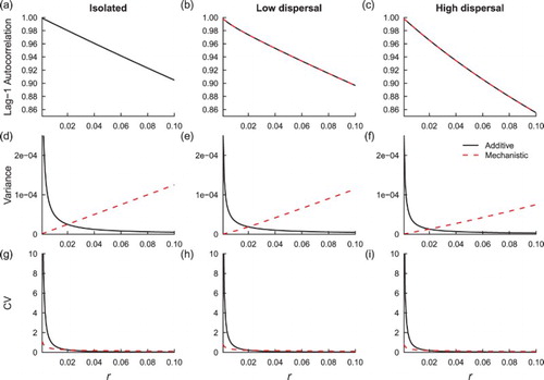
The increasing trend in the lag-1 autocorrelation statistic is independent of noise type, but the noise mechanism influences the patterns in the variability statistics (Figure 2). Variance decreases when environmental noise influences the growth rate parameter, but it increases if noise is additive. The coefficient of variation increases under both noise regimes, but it increases more rapidly under the effect of additive noise than multiplicative noise. In sum, noise type and coupling influence indicator statistics for population extinction.

4. Simulation study procedure

The theoretical predictions for the summary statistics in Section 3 are calculated about the steady state (the subpopulation mean $(x_1^{\ast },x_2^{\ast })=(r,r)$). To test the robustness of the theoretical predictions for the leading indicator statistics under deteriorating environmental conditions, we conducted a simulation study using the fast-slow models derived in Section 2. Using the parameters in Table 1, we simulated 500 stochastic fast-slow models approaching extinction under high and low dispersal regimes, multiplicative and additive noise, and under spatially homogeneous conditions (system (2(2) $\begin{array}{rl}\frac{\mathrm{d}{x}_1}{\mathrm{d}t}& =r{x}_1-x_1^2-m{x}_1+m{x}_2,\\ \frac{\mathrm{d}{x}_2}{\mathrm{d}t}& =r{x}_2-x_2^2-m{x}_2+m{x}_1,\\ \frac{\mathrm{d}r}{\mathrm{d}t}& =-r_0,\end{array}$(2) ) and (3(3) $r\left(t\right)=\{\begin{array}{ll}r-r_{0}t,& t<t^{\ast },\\ 0,& t\ge t^{\ast },\end{array}$(3) )) and heterogeneous environmental conditions (system (4(4) $\begin{array}{rl}\frac{\mathrm{d}{x}_1}{\mathrm{d}t}& =r_1{x}_1-x_1^2-m{x}_1+m{x}_2,\\ \frac{\mathrm{d}{x}_2}{\mathrm{d}t}& =r_2{x}_2-x_2^2-m{x}_2+m{x}_1,\\ \frac{\mathrm{d}{r}_2}{\mathrm{d}t}& =-r_0,\end{array}$(4) ) and (5(5) $r_2\left(t\right)=\{\begin{array}{ll}{r}_2-r_{0}t,& t<t^{\ast },\\ 0,& t\ge t^{\ast },\end{array}$(5) )).

To evaluate the performance of the summary statistics as indicators of population extinction, we processed the time series data for the subpopulations occupying each patch as follows. We used Gaussian filtering to remove the influence of the gradually varying mean [12]. We fitted a Gaussian kernel smoothing function with a fixed bandwidth across each $x_i$ time series up to the time that extinction was predicted in the deteriorating patch ($t^{\ast }$ in Table 1). We obtained the residuals by subtracting the fitted function from each time series. To capture changes in the statistics through time, we calculated the lag-1 autocorrelation, variance and coefficient of variation of the residuals over a moving window half the length of each time series. Lag-1 autocorrelation and variance of each $x_i$ replicate were, respectively, calculated using the acf and var functions in R, and the coefficient of variation was found by calculating the mean and standard deviation of each replicate. To establish the average behaviour of each statistic, we calculated the median and 95% prediction intervals for each of the statistics for each patch over 500 simulations of each model. The prediction intervals were obtained using the quantile function in R. To quantify the degree of association between time and the statistic for each time series, we used Kendall's correlation coefficient τ, a non-parametric statistic of association between two quantities that has values between 1 (representing positive correlation) and $-1$ (negative correlation). Kendall's correlation coefficient was used to quantify the strength of the trend for each realization, and the median value of τ from the 500 simulations of each model was recorded to assess the generality of detectability of statistical patterns. To represent the distribution of Kendall's τ for each set of model simulations, Kendall's τ boxplots were calculated for each model (see the electronic supplementary material for details).

5. Results

5.1. Synchronous system results

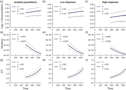
The theoretical predictions for trends in the indicator statistics are robust under a moving window over a suite of simulations. Increases in lag-1 autocorrelation, variance and coefficient of variation are observed from the simulation study of the coupled model with additive noise (Figure 3), whereas increasing lag-1 autocorrelation and coefficient of variation, and decreasing variance are observed as the extinction threshold is approached in the coupled system with multiplicative noise (Figure 4). As predicted from the theory, higher dispersal levels induce decreased magnitude and slope of the trends in the indicator statistics. Under additive noise, median Kendall correlation coefficient values are all positive, indicating that on average, positive trends in indicator statistics occur as extinction is approached, but there is variability in the observed trends of lag-1 autocorrelation and variance (see Figures 1 and 2 in the electronic supplementary material). The reduction in median τ for these statistics suggest that higher dispersal levels weaken the positive relationship with changing intrinsic dynamics. In contrast, the median correlation coefficient calculated from the simulations for the coefficient of variation is close to unity, showing that a strong positive relationship between decreasing intrinsic dynamics and coefficient of variation can be expected under additive noise. This finding is common to all dispersal regimes. Variance exhibits a strong decreasing trend in the systems with multiplicative noise, and the corresponding coefficient of variation signal is not as strong as that observed in the additive noise models (compare the median correlation coefficients). Trends in lag-1 autocorrelation are also slightly weaker in systems with multiplicative noise compared to systems with additive noise. In sum, indicator statistics behave as predicted by the theory, with coefficient of variation performing consistently well as an indicator of critical slowing down across coupling levels and noise regimes.

Figure 3. Simulation study predictions for the summary statistics of the $x_1$ population in a homogeneous coupled system with additive environmental noise. Thick blue lines indicate the median value of each statistic for the $x_1$ population over 500 realizations; thick black lines indicate the median value of each statistic for the $x_2$ population over 500 simulations. Dotted lines indicate the 95% prediction interval for each statistic. The median value of Kendall's correlation coefficient τ is reported for each indicator statistic over 500 simulations. Subfigures (a), (d) and (g) are summary statistic predictions for isolated patches, (b), (e) and (h) are predictions for populations coupled through low dispersal levels, and (c), (f) and (i) are predictions for populations coupled through high dispersal. Parameter values used for the numerical predictions are given in Table 1.

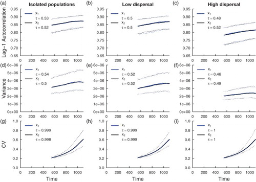
Figure 4. Simulation study predictions for the summary statistics of the $x_1$ population in a homogeneous coupled system with mechanistic environmental noise. Thick blue lines indicate the median value of each statistic for the $x_1$ population over 500 realizations; thick black lines indicate the median value of each statistic for the $x_2$ population over 500 simulations. Dotted lines indicate the 95% prediction interval for each statistic. The median value of Kendall's correlation coefficient τ is reported for each indicator statistic over 500 simulations. Subfigures (a), (d) and (g) are summary statistic predictions for isolated patches, (b), (e) and (h) are predictions for populations coupled through low dispersal levels, and (c), (f) and (i) are predictions for populations coupled through high dispersal. Parameter values used for the numerical predictions are given in Table 1.

5.2. How spatial heterogeneity affects critical slowing down in a spatially extended system

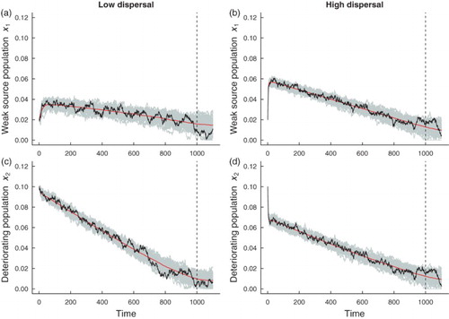
Spatial systems are generally heterogeneous or ‘patchy’ in nature [31], rather than spatially homogeneous. To examine how spatial heterogeneities affect critical slowing down in a spatially extended system, and whether the predictions for the leading indicator statistics for the spatially homogeneous model are robust to heterogeneities, we considered two fast-slow spatially heterogeneous models with additive noise. We assumed that environmental conditions remain constant in patch 1, while conditions in patch 2 deteriorate. We investigated the dynamics when patch 1 is a ‘strong source’ patch, that is, patch quality is good and conditions are favourable for population growth. We also investigated the onset of critical slowing down when patch 1 is a ‘weak source patch’, that is, when conditions are poor for population growth, and the population is close to extinction. Figure 5 shows simulations of the fast-slow model with a strong source patch and a deteriorating patch under low and high dispersal. Due to mixing, subpopulations in both patches decline. The presence of the good patch prevents deterioration to population extinction in the second patch. Although the second patch deteriorates at the same rate as the deteriorating patches in the spatially homogeneous system, the good source patch promotes a strong ‘rescue effect’. Under the higher dispersal regime, the populations in each patch decline at similar rates due to the high level of mixing between subpopulations (Figure 5(b, d)). Similar patterns of subpopulation decline due to high levels of coupling are also observed when patch 1 is a poor quality environment (Figure 6(b, d)). When a poor quality patch is coupled to a deteriorating subpopulation, both subpopulations decline towards extinction and exhibit larger fluctuations compared to subpopulations where one patch offers a good quality environment (compare Figures 5 with 6). The weak source patch does not promote a rescue effect, even for higher levels of coupling. The spatially heterogeneous metapopulation with a weak source patch appears to be more responsive to the intrinsic dynamics in each patch because there is an initial transient in each patch before the system relaxes to the moving steady state of the fast-slow system (Figure 6). Initially, the subpopulation in patch 1 is buffered from extinction due to dispersal of individuals from patch 2, whose subpopulation initially has a greater intrinsic growth rate than the patch 2 subpopulation.

Figure 5. Simulations of the $x_1$ and $x_2$ populations, in a heterogeneous coupled patch system with additive noise and a static patch with a good environment (‘strong source’ patch). The red line shows the mean of the 500 $x_i$ realizations of the heterogeneous model, a single realization (black line) and 50 simulations of each subpopulation $x_i$ are shown in gray. The dashed vertical line indicates the time that the transcritical bifurcation occurs. Subfigures (a) and (c) are simulations of populations coupled through low dispersal levels, and (b) and (d) are simulations of populations coupled through high dispersal. Numerical values for the parameters used in the simulations are provided in Table 1.

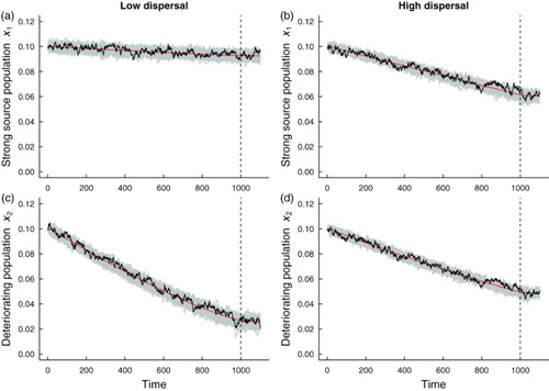
Figure 6. Simulations of the $x_1$ and $x_2$ populations, in a heterogeneous coupled patch system with additive noise and a bad environment (‘weak source’ patch). The red line shows the mean of the 500 $x_i$ realizations of the heterogeneous model, a single realization (black line) and 50 simulations of each subpopulation $x_i$ are shown in gray. A transient is observed before the system relaxes to the moving fast-slow steady state. The dashed vertical line indicates the time that the transcritical bifurcation occurs. Subfigures (a) and (c) are simulations of populations coupled through low dispersal levels, and (b) and (d) are simulations of populations coupled through high dispersal. Numerical values for the parameters used in the simulations are provided in Table 1.

Figures 5 and 6 suggest the following hypothesis: as a consequence of a rescue effect, temporal indicators of critical slowing down should be weaker in a spatially heterogeneous system with a strong source patch than a spatially heterogeneous system with a weak source patch. The latter system is closer to the extinction threshold, whereas the metapopulation with a strong source patch is saved from extinction.

5.2.1. Theoretical predictions for leading indicators of extinction in spatially heterogeneous systems

To examine the behaviour of leading indicators of extinction in a spatially heterogeneous system, we numerically integrated equations (22(22) $S_1\left(\omega \right)=\frac{D_{11}{a}_{22}^2+D_{22}{a}_{12}^2+D_{11}{\omega }^2}{({\omega }^2-d{)}^2+T^2{\omega }^2}.$(22) ) and (23(23) $S_2\left(\omega \right)=\frac{D_{22}{a}_{11}^2+D_{11}{a}_{21}^2+D_{22}{\omega }^2}{({\omega }^2-d{)}^2+T^2{\omega }^2}.$(23) ) for each steady-state value $(x_1^{\ast },x_2^{\ast })$ of system (1(1) $\begin{array}{rl}\frac{\mathrm{d}{x}_1}{\mathrm{d}t}& =r_1{x}_1-x_1^2-m{x}_1+m{x}_2,\\ \frac{\mathrm{d}{x}_2}{\mathrm{d}t}& =r_2{x}_2-x_2^2-m{x}_2+m{x}_1,\end{array}$(1) ) (which we took to represent the mean of the stochastic fast-slow system) for $r_2$ values ranging between 0.1 and ${10}^{-3}$, while $r_1$ remained constant (Table 1) and used the integrals to calculate summary statistics. Figures 7 and 8 show the behaviour of the summary statistics as $r_2$ decreases towards zero from the right. Similar to the spatially homogeneous system with additive noise, the lag-1 autocorrelation function, variance and coefficient of variation all increase, in both patches, as environmental conditions in patch 2 deteriorate. Moreover, trends in leading indicators are dampened with increasing dispersal, just as predicted by the analysis of the spatially homogenous system.

Figure 7. Theoretical predictions for the summary statistics of a heterogeneous coupled system with additive noise and a static patch with a good environment (‘strong source’ patch). Subfigures (a), (c) and (e) are summary statistic predictions for $x_1$ and $x_2$ subpopulations coupled through low dispersal levels, and (b), (d) and (f) are predictions for subpopulations coupled through high dispersal. Parameter values used for the numerical predictions are given in Table 1. Predictions were calculated for fluctuations about the steady state $(x_1^{\ast },x_2^{\ast })$ of system (1(1) $\begin{array}{rl}\frac{\mathrm{d}{x}_1}{\mathrm{d}t}& =r_1{x}_1-x_1^2-m{x}_1+m{x}_2,\\ \frac{\mathrm{d}{x}_2}{\mathrm{d}t}& =r_2{x}_2-x_2^2-m{x}_2+m{x}_1,\end{array}$(1) ) (representing the mean of the stochastic fast-slow system) for $r_2$ values ranging from 0.1 down to ${10}^{-3}$, in increments of ${10}^{-3}$, while $r_1$ remained constant at 0.1.

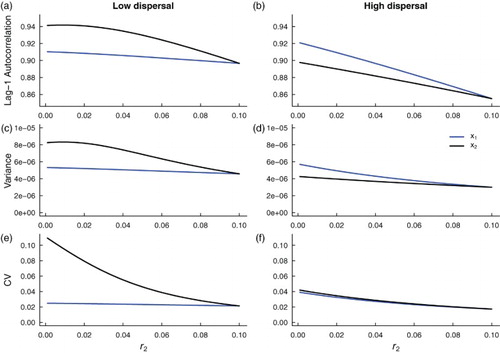
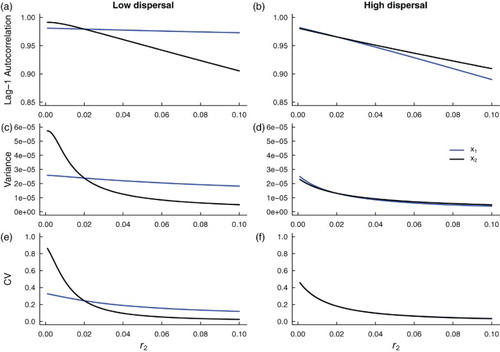
Figure 8. Theoretical predictions for the summary statistics of a heterogeneous coupled system with additive noise and a static patch with a bad environment (‘weak source’ patch). Subfigures (a), (c) and (e) are summary statistic predictions for $x_1$ and $x_2$ subpopulations coupled through low dispersal levels, and (b), (d) and (f) are predictions for subpopulations coupled through high dispersal. Parameter values used for the numerical predictions are given in Table 1. Predictions were calculated for fluctuations about the steady state $(x_1^{\ast },x_2^{\ast })$ of system (1(1) $\begin{array}{rl}\frac{\mathrm{d}{x}_1}{\mathrm{d}t}& =r_1{x}_1-x_1^2-m{x}_1+m{x}_2,\\ \frac{\mathrm{d}{x}_2}{\mathrm{d}t}& =r_2{x}_2-x_2^2-m{x}_2+m{x}_1,\end{array}$(1) ) (representing the mean of the stochastic fast-slow system) for $r_2$ values ranging from 0.1 down to ${10}^{-3}$, in increments of ${10}^{-3}$, while $r_1$ remained constant at 0.02.

It is also interesting to compare the temporal signals obtained from subpopulation fluctuations in each patch. Since conditions in patch 2 are deteriorating, it is reasonable to expect that subpopulation $x_2$ would exhibit a stronger signal of critical slowing down than the $x_1$ subpopulation subject to a constant growth rate in patch 1, but this is not always the case, because coupling the subpopulations in a metapopulation dampens the signals. Under low dispersal and good quality conditions in patch 1, $x_2$ exhibits a stronger signal of critical slowing down than $x_1$, as indicated by the magnitude and slope of the summary statistics (Figure 7(a,c,e)), but $x_1$ exhibits more elevated signals of critical slowing down than $x_2$ when coupling is high (Figure 7(b,d,f)). Here, the good quality patch 1 acts to buffer subpopulation 2 from extinction through high levels of dispersal between patches.

Under high dispersal and bad quality conditions in patch 2, patterns in leading indicators are similar in both patches (Figure 8(b,d,f)). Intrinsic dynamics in each patch become more similar as patch 2 conditions deteriorate. When migration between patches is low, leading indicators obtained from population fluctuations in patch 2 change more rapidly than those obtained from patch 1 as $r_2$ approaches zero from the right. Further away from the extinction point at $r_2=0$, patch 1 has larger variance, lag-1 autocorrelation and coefficient of variation due to poor conditions that make the $x_1$ subpopulation closer to extinction. All of the summary statistics increase, in both patches, as $r_2$ approaches zero.

Comparing magnitudes of the signals in Figures 7 and 8, we observe stronger signals of critical slowing down in the summary statistics obtained from the weak-source-patch spatially heterogeneous model than the model with a good quality patch. These predictions suggest that the spatially heterogeneous system with a weak source patch, which is close to extinction, should exhibit stronger signals of critical slowing down than the model with a good source patch that promotes metapopulation persistence.

5.2.2. Simulation study predictions for leading indicators of extinction in spatially heterogeneous systems

Predictions for the summary statistics calculated from the spatially heterogeneous fast-slow models over a moving window (Figures 9 and 10) agree with the predicted trends obtained through numerical integration (Figures 7 and 8). From the median τ values, positive associations between each of the leading indicators and time are predicted, but there is considerably more variability in leading indicator trends than those obtained from simulations of the spatially homogeneous system (compare the median Kendall's τ values in Figure 3 with those Figures 9 and 10). Moreover, the prediction that stronger signals of critical slowing down are observed in the spatially heterogeneous system with a weak source patch than the corresponding system with a strong source patch is robust in the simulated fast-slow models (compare τ-values in Figure 9 with those in Figure 10). Just as in the spatially homogeneous system, the coefficient of variation appears to be the most reliable indicator of extinction.

Figure 9. Simulation study predictions for the summary statistics of the $x_1$ and $x_2$ population in a heterogeneous coupled system with additive environmental noise and a static patch with a good environment (‘strong source’ patch). Thick blue lines indicate the median value of each statistic for the $x_1$ population over 500 realizations; thick black lines indicate the median value of each statistic for the $x_2$ population over 500 simulations. Dotted lines indicate the 95% prediction interval for each statistic. The median value of Kendall's correlation coefficient τ is reported for each indicator statistic over 500 simulations. Subfigures (a), (c) and (e) are predictions for populations coupled through low dispersal levels, and (b), (d) and (f) are predictions for populations coupled through high dispersal. Parameter values used for the numerical predictions are given in Table 1.

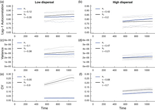
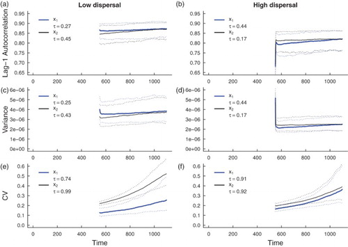
Figure 10. Simulation study predictions for the summary statistics of the $x_1$ and $x_2$ population in a heterogeneous coupled system with additive environmental noise and a static patch with a bad environment (‘weak source’ patch). Thick blue lines indicate the median value of each statistic for the $x_1$ population over 500 realizations; thick black lines indicate the median value of each statistic for the $x_2$ population over 500 simulations. Dotted lines indicate the 95% prediction interval for each statistic. The median value of Kendall's correlation coefficient τ is reported for each indicator statistic over 500 simulations. Subfigures (a), (c) and (e) are predictions for populations coupled through low dispersal levels, and (b), (d) and (f) are predictions for populations coupled through high dispersal. Parameter values used for the numerical predictions are given in Table 1. Initial transient behaviour of $x_1$ and $x_2$ (Figure 6) is captured by the sharp change in statistics over the moving window.

6. Discussion

Anticipating critical transitions in spatially extended systems is a complex task. Temporal, patch-specific indicators are potentially useful for predicting extinction events in multi-patch systems with low mixing between sites and environmental stochasticity. We developed a stochastic fast-slow two-patch model appropriate for various noise regimes and environmental conditions. We used the static model to derive leading indicators of extinction particular to each patch. Through simulating the stochastic fast-slow models, we showed that predicted trends in the leading indicators are robust, and therefore, critical slowing down prior to population extinction is detectable.

Noise, coupling and return rates to the steady state together determine temporal summary statistics for the two-patch model studied here. Using a spatially homogeneous model, we showed that increasing the level of coupling between patches dampens signals by decreasing their magnitude relative to those obtained for isolated populations. Additionally, the framework presented here accounts for the fact that environmental stochasticity can impact a population in different ways - by either affecting the entire patch growth rate, or a specific parameter in the system, for example, vital rates such as intrinsic growth rate. Noise regimes affect the trends in variance, with additive noise inducing rising variance, whereas noise that scales with population density induces declining variance. On the other hand, the lag-1 autocorrelation function is independent of the noise regime, but exhibits non-monotonic behaviour with increasing coupling strength. Coupling patches through moderate levels of dispersal predicted a lower patch-specific lag-1 autocorrelation than that for isolated populations, but sufficiently high dispersal predicted an autocorrelation comparable to that of isolated populations, as the metapopulation becomes well-mixed enough to behave as a single patch, and population dynamics become synchronous across patches. The simulation study suggested that the coefficient of variation is the most robust temporal indicator across different noise and coupling regimes, and environmental conditions. As the critical threshold for extinction is approached, the population mean decreases to zero at a faster rate than the rate of change of its standard deviation, and consequently, the coefficient of variation is expected to blow up. These predictions for the behaviour of the leading indicators are robust even when the condition of spatial homogeneity is relaxed. The analytical expressions derived in the homogeneous case are a useful approximation for their predictive capability in spatially heterogenous systems, where having patch-specific indicators that account for coupling between units becomes more important.

Increasing the degree of coupling induces synchronous dynamics in the two patches in the heterogeneous model. When a good quality patch forms part of the spatially extended system, rescue effects through dispersal save the metapopulation from extinction by bringing the dynamics of the deteriorating quality patch and the good quality patch into synchrony. Alternatively, in the weak-source-patch heterogeneous system, the population dynamics of the poor quality patch are synchronized with that of the deteriorating subpopulation over a short time frame, and both subpopulations simultaneously decrease to the critical threshold. These results suggest that both patches in the system need to be monitored, not just a patch where there is a known deterioration in environmental conditions. Having patch-specific predictions is useful, since population dynamics in both patches will exhibit critical slowing down.

To capture the non-stationarity of local dynamics in the metapopulation, we used a fast-slow framework to model gradual changes in environmental conditions in each patch. Singularly perturbed models united with various forms of stochasticity offer a natural framework for modelling non-stationary dynamics that change over long time scales. Understanding the near-critical dynamics of these types of models is an underdeveloped area of mathematical ecology (but see Zhu et al. [51]). We evaluated the leading indicator statistics about the steady state, and then we chose a sufficiently slow rate of change of the intrinsic growth rate in each patch so that the numerical solution of the fast-slow model is sufficiently close to the steady state for each growth rate value. More research is needed to identify at what value of $r_0$ does the validity of this assumption break down. Fast-slow models are known to exhibit bifurcation delays characterized by scaling laws [28, 51]. Obtaining analytical expressions or approximations for the extinction-time distribution is an important problem that needs further research, and in particular, in heterogeneous multi-patch systems.

We used a simple model for a transcritical bifurcation to describe the intrinsic patch dynamics but the framework could be extended in many ways. Saddle-node bifurcations are the deterministic skeleton beneath many critical transitions in ecology (e.g. bistable ecosystems [5, 11, 32, 48]). We expect that the predictions for dampening of the indicator statistics under increased coupling would hold for spatial systems with saddle-node bifurcation dynamics in each patch, but the effects of noise and other heterogeneities on leading indicator predictions is not clear. Our approach did not account for environmental variations that drive seasonality in biotic variables (e.g. recruitment, resource availability) and abiotic variables (e.g. temperature, precipitation). Additionally, environmental noise is often correlated in time, inducing correlated population fluctuations (spatial autocorrelation in ecology [26] or Moran effects [21]). Accounting for spatial structure and movement pathways through networks [41, 43] is another natural extension of the 2-patch model presented here. Moreover, early warning signal predictions could be different for alternative coupling patterns such as density-dependent dispersal (e.g. [1, 45].

In conclusion, we have developed new theory for early warning systems of critical transitions in metapopulations. We have studied a general model for populations approaching extinction that can be readily adapted to different extinction and elimination situations. We have shown that coupling between patches and spatial heterogeneity dampen statistical early warning signals of an impending bifurcation. Although the analytical expressions for leading indicators have to be evaluated numerically for the spatially heterogeneous model, they still form part of a useful theory for identification of critical slowing down in multi-patch systems.

Acknowledgements

E O'Dea, J Drake and an anonymous reviewer provided valuable comments on the manuscript.

Disclosure statement

No potential conflict of interest was reported by the author.

ORCID

Suzanne M. O'Regan http://orcid.org/0000-0002-9446-955X

Additional information

Funding

Much of this work was conducted while a Postdoctoral Fellow at the National Institute for Mathematical and Biological Synthesis, an Institute sponsored by the National Science Foundation through NSF Award # DBI-1300426, with additional support from The University of Tennessee, Knoxville.

Appendix

The spectral density of a Fourier-transformed signal $z\left(t\right)$ is formally defined as $S\left(\omega \right)=\underset{T\to \mathrm{\infty }}{lim}\frac{1}{T}E\left\{|\tilde{z}\right(\omega \left){|}^2\right\}.$ To obtain the spectral density $S_1\left(\omega \right)$ from Equation (21(21) $\widetilde{z_1}\left(\omega \right)=\frac{(a_{22}-i\omega )\sqrt{D_{11}}{\mathrm{\Gamma }}_1\left(\omega \right)}{d-{\omega }^2-iT\omega }-\frac{a_{12}\sqrt{D_{22}}{\mathrm{\Gamma }}_2\left(\omega \right)}{d-{\omega }^2-iT\omega },$(21) ), we calculate, $\begin{array}{rl}{S}_1\left(\omega \right)& =\underset{T\to \mathrm{\infty }}{lim}\frac{1}{T}E\left[|z_1\right(\omega \left){|}^2\right]\\ & =\underset{T\to \mathrm{\infty }}{lim}\frac{1}{T}\left[{\left|\frac{(a_{22}-i\omega )\sqrt{D_{11}}}{d-{\omega }^2-iT\omega }\right|}^{2}E\right(|{\mathrm{\Gamma }}_1\left(\omega \right){|}^2)+{|-\frac{a_{12}\sqrt{D_{22}}}{d-{\omega }^2-iT\omega }|}^{2}E(|{\mathrm{\Gamma }}_2\left(\omega \right){|}^2)\\ & \phantom{{\left|\frac{(a_{22}-i\omega )\sqrt{D_{11}}}{d-{\omega }^2-iT\omega }\right|}^2}+|-\frac{a_{12}\sqrt{D_{22}}}{d-{\omega }^2-iT\omega }|\left|\frac{(a_{22}-i\omega )\sqrt{D_{11}}}{d-{\omega }^2-iT\omega }\right|E\left\{\widehat{{\mathrm{\Gamma }}_1}\right(\omega \left){\mathrm{\Gamma }}_2\right(\omega )+{\mathrm{\Gamma }}_1(\omega \left)\widehat{{\mathrm{\Gamma }}_2}\right(\omega \left)\right\}],\end{array}$ where $\widehat{{\mathrm{\Gamma }}_i}\left(\omega \right)$ denotes the complex conjugate. Since ${\mathrm{\Gamma }}_1\left(\omega \right)$ and ${\mathrm{\Gamma }}_2\left(\omega \right)$ are uncorrelated, then $E\left(\widehat{{\mathrm{\Gamma }}_1}\right(\omega \left){\mathrm{\Gamma }}_2\right(\omega \left)\right)=E\left(\widehat{{\mathrm{\Gamma }}_2}\right(\omega \left){\mathrm{\Gamma }}_1\right(\omega \left)\right)=0$. We note that $\underset{T\to \mathrm{\infty }}{lim}\frac{1}{T}E\left(|{\mathrm{\Gamma }}_i\right(\omega \left){|}^2\right)=1,$ since ${\mathrm{\Gamma }}_i\left(\omega \right)$ denotes the Fourier transform of a Wiener process, and the spectral density of a Wiener process is unity because all frequencies are equally represented in the density. Similarly, $\begin{array}{rl}{S}_2\left(\omega \right)& =\underset{T\to \mathrm{\infty }}{lim}\frac{1}{T}E\left[|z_2\right(\omega \left){|}^2\right]\\ & =\underset{T\to \mathrm{\infty }}{lim}\frac{1}{T}\left[{\left|\frac{(a_{11}-i\omega )\sqrt{D_{22}}}{d-{\omega }^2-iT\omega }\right|}^{2}E\right(|{\mathrm{\Gamma }}_1\left(\omega \right){|}^2)+{|-\frac{a_{21}\sqrt{D_{11}}}{d-{\omega }^2-iT\omega }|}^{2}E(|{\mathrm{\Gamma }}_2\left(\omega \right){|}^2)\\ & \phantom{{\left|\frac{(a_{11}-i\omega )\sqrt{D_{22}}}{d-{\omega }^2-iT\omega }\right|}^2}+|-\frac{a_{21}\sqrt{D_{11}}}{d-{\omega }^2-iT\omega }|\left|\frac{(a_{11}-i\omega )\sqrt{D_{22}}}{d-{\omega }^2-iT\omega }\right|E\left\{\widehat{{\mathrm{\Gamma }}_1}\right(\omega \left){\mathrm{\Gamma }}_2\right(\omega )+{\mathrm{\Gamma }}_1(\omega \left)\widehat{{\mathrm{\Gamma }}_2}\right(\omega \left)\right\}]\\ & =\frac{D_{22}{a}_{11}^2+D_{11}{a}_{21}^2+D_{22}{\omega }^2}{({\omega }^2-d{)}^2+T^2{\omega }^2}.\end{array}$

References

- K.C. Abbott, A dispersal-induced paradox: Synchrony and stability in stochastic metapopulations, Ecol. Lett. 14 (2011), pp. 1158–1169. doi: 10.1111/j.1461-0248.2011.01670.x
- L.J.S. Allen, An Introduction to Stochastic Processes with Applications to Biology, Prentice Hall, Upper Saddle River, NJ, 2003.
- E.J. Allen, L.J.S. Allen, A. Arciniega, and P.E. Greenwood, Construction of Equivalent Stochastic Differential Equation Models, Stoch. Anal. Appl. 26 (2008), pp. 274–297. doi: 10.1080/07362990701857129
- S. Battiston, J.D. Farmer, A. Flache, D. Garlaschelli, A.G. Haldane, H. Heesterbeek, C. Hommes, C. Jaeger, R. May, and M. Scheffer, Complexity theory and financial regulation, Science 351 (2016), pp. 818–819. doi: 10.1126/science.aad0299
- B. Beisner, D. Haydon, and K. Cuddington, Alternative stable states in ecology, Front. Ecol. Environ. 1 (2003), pp. 376–382. doi: 10.1890/1540-9295(2003)001[0376:ASSIE]2.0.CO;2
- G. Bel, A. Hagberg, and E. Meron, Gradual regime shifts in spatially extended ecosystems, Theor. Ecol. 5 (2012), pp. 591–604. doi: 10.1007/s12080-011-0149-6
- C. Boettiger, N. Ross, and A. Hastings, Early warning signals: The charted and uncharted territories, Theor. Ecol. 6 (2013), pp. 255–264. doi: 10.1007/s12080-013-0192-6
- S.R. Carpenter and W.A. Brock, Early warnings of regime shifts in spatial dynamics using the discrete Fourier transform, Ecosphere 1 (2010), p. art10. Available at http://www.esajournals.org/doi/abs/10.1890/ES10-00016.1. doi: 10.1890/ES10-00016.1
- S.R. Carpenter, J.J. Cole, M.L. Pace, R. Batt, W.A. Brock, T. Cline, J. Coloso, J.R. Hodgson, J.F. Kitchell, D.A. Seekell, L. Smith, and B. Weidel, Early warnings of regime shifts: A whole-ecosystem experiment, Science 332 (2011), pp. 1079–1082. doi: 10.1126/science.1203672
- L. Dai, K.S. Korolev, and J. Gore, Slower recovery in space before collapse of connected populations, Nature 496 (2013), pp. 355–358. doi: 10.1038/nature12071
- L. Dai, D. Vorselen, K.S. Korolev, and J. Gore, Generic indicators for loss of resilience before a tipping point leading to population collapse, Science 336 (2012), pp. 1175–1177. doi: 10.1126/science.1219805
- V. Dakos, M. Scheffer, E.H. van Nes, V. Brovkin, V. Petoukhov, and H. Held, Slowing down as an early warning signal for abrupt climate change, Proc. Natl. Acad. Sci. USA 105 (2008), pp. 14308–14312. doi: 10.1073/pnas.0802430105
- V. Dakos, E.H. van Nes, R. Donangelo, H. Fort, and M. Scheffer, Spatial correlation as leading indicator of catastrophic shifts, Theor. Ecol. 3 (2010), pp. 163–174. doi: 10.1007/s12080-009-0060-6
- V. Dakos, S.R. Carpenter, W.A. Brock, A.M. Ellison, V. Guttal, A.R. Ives, S. Kefi, V. Livina, D.A. Seekell, E.H. van Nes, and M. Scheffer, Methods for detecting early warnings of critical transitions in time series illustrated using simulated ecological data, PLoS One 7 (2012), p. e41010. doi: 10.1371/journal.pone.0041010
- J.M. Drake and B.D. Griffen, Early warning signals of extinction in deteriorating environments, Nature 467 (2010), pp. 456–459. doi: 10.1038/nature09389
- N. Fenichel, Geometric singular perturbation theory for ordinary differential equations, J. Differential Equations 31 (1979), pp. 53–98. doi: 10.1016/0022-0396(79)90152-9
- C.W. Gardiner, Handbook of Stochastic Methods for Physics, Chemistry and the Natural Sciences, Springer, Berlin, 2004.
- V. Guttal and C. Jayaprakash, Spatial variance and spatial skewness: Leading indicators of regime shifts in spatial ecological systems, Theor. Ecol. 2 (2009), pp. 3–12. doi: 10.1007/s12080-008-0033-1
- A.G. Haldane and R.M. May, Systemic risk in banking ecosystems, Nature 469 (2011), pp. 351–355. doi: 10.1038/nature09659
- R.D. Holt, Population dynamics in two-patch environments: Some anomalous consequences of an optimal habitat distribution, Theor. Popul. Biol. 28 (1985), pp. 181–208. doi: 10.1016/0040-5809(85)90027-9
- P.J. Hudson and I.M. Cattadori, The Moran effect: A cause of population synchrony, Trends Ecol. Evol. 14 (1999), pp. 1–2. doi: 10.1016/S0169-5347(98)01498-0
- A.R. Ives and V. Dakos, Detecting dynamical changes in nonlinear time series using locally linear state-space models, Ecosphere 3 (2012). Article 58. doi: 10.1890/ES11-00347.1
- A.R. Ives, B. Dennis, K.L. Cottingham, and S.R. Carpenter, Estimating community stability and ecological interactions from time series data, Ecol. Monogr. 73 (2003), pp. 301–330. doi: 10.1890/0012-9615(2003)073[0301:ECSAEI]2.0.CO;2
- V.A.A. Jansen and A.L. Lloyd, Local stability analysis of spatially homogeneous solutions of multi-patch systems, J. Math. Biol. 41 (2000), pp. 232–252. doi: 10.1007/s002850000048
- S. Kéfi, V. Guttal, W.A. Brock, S.R. Carpenter, A.M. Ellison, V.N. Livina, D.A. Seekell, M. Scheffer, E.H. van Nes, and V. Dakos, Early warning signals of ecological transitions: Methods for spatial patterns, PloS One 9 (2014), p. e92097. doi: 10.1371/journal.pone.0092097
- W.D. Koenig, Spatial autocorrelation of ecological phenomena, Trends Ecol. Evol. 14 (1999), pp. 22–26. doi: 10.1016/S0169-5347(98)01533-X
- M.A. Kramer, W. Truccolo, U.T. Eden, K.Q. Lepage, L.R. Hochberg, E.N. Eskandar, J.R. Madsen, J.W. Lee, A. Maheshwari, E. Halgren, C.J. Chu, and S.S. Cash, Human seizures self-terminate across spatial scales via a critical transition, Proc. Natl. Acad. Sci. 109 (2012), pp. 21116–21121. doi: 10.1073/pnas.1210047110
- C. Kuehn, A mathematical framework for critical transitions: Bifurcations, fast-slow systems and stochastic dynamics, Phys. D 240 (2011), pp. 1020–1035. doi: 10.1016/j.physd.2011.02.012
- C. Kuehn, Multiple Time Scale Dynamics, Springer International Publishing, Switzerland, 2015.
- T.M. Lenton, Early warning of climate tipping points, Nat. Climate Change 1 (2011), pp. 201–209. doi: 10.1038/nclimate1143
- S.A. Levin, Population dynamic models in heterogeneous environments, Annu. Rev. Ecol. Syst. 7 (1976), pp. 287–310. doi: 10.1146/annurev.es.07.110176.001443
- D. Ludwig, D.D. Jones, and C.S. Holling, Qualitative analysis of insect outbreak systems: The spruce budworm and forest, J. Anim. Ecol. 47 (1978), pp. 315–332. doi: 10.2307/3939
- R.M. Nisbet and W.S.C. Gurney, Modelling Fluctuating Populations, Wiley, New York, 1982.
- S.M. O'Regan and J.M. Drake, Theory of early warning signals of disease emergence and leading indicators of elimination, Theor Ecol 6 (2013), pp. 333–357. doi: 10.1007/s12080-013-0185-5
- S.M. O'Regan, J.W. Lillie, and J.M. Drake, Leading indicators of mosquito-borne disease elimination, Theoretical Ecology 9 (2016), pp. 269–286. doi: 10.1007/s12080-015-0285-5
- T. Quail, A. Shrier, and L. Glass, Predicting the onset of period-doubling bifurcations in noisy cardiac systems, Proceedings of the National Academy of Sciences of the United States of America 112 (2015), pp. 9358–9363. doi: 10.1073/pnas.1424320112
- R. Quax, D. Kandhai, and P.M.A. Sloot, Information dissipation as an early-warning signal for the Lehman Brothers collapse in financial time series, Scientific Reports 3 (2013), p. 1898. doi: 10.1038/srep01898
- M. Scheffer, Critical Transitions in Nature and Society, Princeton University Press, Princeton, NJ, 2009.
- M. Scheffer, J. Bascompte, W.A. Brock, V. Brovkin, S.R. Carpenter, V. Dakos, H. Held, E.H. van Nes, M. Rietkerk, and G. Sugihara, Early warning signals for critical transitions, Nature 461 (2009), pp. 53–59. doi: 10.1038/nature08227
- M. Scheffer, S.R. Carpenter, V. Dakos, and E.H. van Nes, Generic indicators of ecological resilience: Inferring the chance of a critical transition, Annu. Rev. Ecol. Evol. Syst. 46 (2015), pp. 145–167. doi: 10.1146/annurev-ecolsys-112414-054242
- M. Scheffer, S.R. Carpenter, T.M. Lenton, J. Bascompte, W. Brock, V. Dakos, J. van de Koppel, I.A. van de Leemput, S.A. Levin, E.H. van Nes, M. Pascual, and J. Vandermeer, Anticipating critical transitions, Science 338 (2012), pp. 344–348. doi: 10.1126/science.1225244
- S.H. Strogatz, Nonlinear Dynamics and Chaos with Applications to Physics, Biology, Chemistry and Engineering, Addison-Wesley, Reading, MA, 1994.
- S. Suweis and P. D'Odorico, Early warning signs in social-ecological networks, PloS One 9 (2014), p. e101851. doi: 10.1371/journal.pone.0101851
- C. Trefois, P.M. Antony, J. Goncalves, A. Skupin, and R. Balling, Critical transitions in chronic disease: Transferring concepts from ecology to systems medicine, Current Opinion in Biotechnology 34 (2015), pp. 48–55. doi: 10.1016/j.copbio.2014.11.020
- E. Tromeur, L. Rudolf, and T. Gross, Impact of dispersal on the stability of metapopulations, J. Theor. Biol. 392 (2015), pp. 1–11. doi: 10.1016/j.jtbi.2015.11.029
- I.A. van de Leemput, M. Wichers, A.O.J. Cramer, D. Borsboom, F. Tuerlinckx, P. Kuppens, E.H. van Nes, W. Viechtbauer, E.J. Giltay, S.H. Aggen, C. Derom, N. Jacobs, K.S. Kendler, H.L.J. van der Maas, M.C. Neale, F. Peeters, E. Thiery, P. Zachar, and M. Scheffer, Critical slowing down as early warning for the onset and termination of depression, Proc. Natl. Acad. Sci. 111 (2014), pp. 87–92. doi: 10.1073/pnas.1312114110
- E.H. van Nes and M. Scheffer, Slow recovery from perturbations as a generic indicator of a nearby catastrophic shift, Am. Nat. 169 (2007), pp. 738–747. doi: 10.1086/516845
- A.J. Veraart, E.J. Faassen, V. Dakos, E.H. van Nes, M. Lürling, and M. Scheffer, Recovery rates reflect distance to a tipping point in a living system, Nature 481 (2012), pp. 357–359.
- P. Villa Martín, J.A. Bonachela, S.A. Levin, and M.A. Muñoz, Eluding catastrophic shifts, Proc. Natl. Acad. Sci. USA 112 (2015), pp. E1828–E1836. doi: 10.1073/pnas.1414708112
- C. Wissel, A universal law of the characteristic return time near thresholds, Oecologia 65 (1984), pp. 101–107. doi: 10.1007/BF00384470
- J. Zhu, R. Kuske, and T. Erneux, Tipping points near a delayed saddle node bifurcation with periodic forcing, SIAM J. Appl. Dyn. Syst. 14 (2015), pp. 2030–2068. doi: 10.1137/140992229