Understanding the effects of intermittent shedding on the transmission of infectious diseases: example of salmonellosis in pigs

ABSTRACT

A number of environmentally transmitted infectious diseases are characterized by intermittent infectiousness of infected hosts. However, it is unclear whether intermittent infectiousness must be explicitly accounted for in mathematical models for these diseases or if a simplified modelling approach is acceptable. To address this question we study the transmission of salmonellosis between penned pigs in a grower-finisher facility. The model considers indirect transmission, growth of free-living Salmonella within the environment, and environmental decontamination. The model is used to evaluate the role of intermittent fecal shedding by comparing the behaviour of the model with constant versus intermittent infectiousness. The basic reproduction number, ${\mathcal{R}}_0$, is used to determine the long-term behaviour of the model regarding persistence or extinction of infection. The short-term behaviour of the model, relevant to swine production, is considered by examining the prevalence of infection at slaughter. Comparison of the two modelling approaches indicates that neglecting the intermittent pattern of infectiousness can result in biased estimates for ${\mathcal{R}}_0$ and infection prevalence at slaughter. Therefore, models for salmonellosis or similar infections should explicitly account for the mechanism of intermittent infectiousness.

KEYWORDS:

• Salmonellosis
• intermittent shedding
• grower-finisher pig
• epidemiology

AMS SUBJECT CLASSIFICATION:

• 92B05
• 34A34

1. Introduction

There are several infectious agents (e.g. Escherichia coli O157:H7, Listeria monocytogenes, Salmonella spp., Toxoplasma gondii, Hepatitis E virus, and Avian Influenza virus) which are characterized with environmental transmission whereby the infectious agents are transmitted through the contaminated environment [11,14,16,24,25,32,35,43]. For such infectious agents, the infectious hosts typically shed the pathogen through their contaminated feces or urine which contributes to the number of free-living pathogens (FLPs) in the environment. Rather than acquiring the infection through a direct contact with an infectious host, for environmentally transmitted infections the susceptible hosts become infected by contacting such infectious agents in a contaminated environment such as food, water, soil, or fomites [7,8,40]. FLPs are capable of survival and possibly growth within the environment [6,27]. Additionally, FLPs may be removed from the environment by natural decay and decontamination practices (e.g. cleaning).

Salmonellosis is the most common foodborne illness in the United States [31,37] with non-typhoidal Salmonella estimated to cause 1.03 million cases of foodborne infection, including 378 deaths, annually [37]. Contaminated pork products have been identified as a source of human salmonellosis [23]. In fact, nearly $14\mathrm{\%}$ of all reported foodborne outbreaks of salmonellosis are the result of contaminated pork products [19]. Thus, reducing the number of salmonellosis cases among pigs in grower-finisher operations can reduce the risk of pork contamination at the time of slaughter, and thereby reduce the number of human cases and fatalities.

Most grower-finisher pig operations follow an all-in/all-out system of production in which a single group of pigs are purchased and fattened over a period of approximately 150 days before being sold for slaughter [18,22]. During this time, pigs may acquire salmonellosis by ingesting free-living Salmonella from the environment, including FLP on the contaminated hides of other pigs. Once infected, pigs begin to shed Salmonella into the environment through their feces [38,45]. Identifying infected pigs can be difficult since most animals are asymptomatic [18,33,34]. The identification of infected pigs is further complicated by an intermittent fecal shedding pattern in which infected pigs cycle through stages of active shedding and non-shedding (here non-shedding may mean a true absence of shedding or an apparent non-shedding where shedding is present but it occurs at very low levels that are below the detection limit) [18,22]. Since transmission of infection occurs primarily through the contaminated environment, many grower-finisher farms implement some form of environmental decontamination (i.e. cleaning) to reduce the risk of infection. Typically, decontamination consists of removing fecal waste from pig pens. Feces removal systems commonly used in practice include scraping and washing of pen floors and the use of pens with slatted floors which allow feces to fall into a pit underneath [18].

In an effort to understand the dynamics of salmonellosis among pigs, several epidemic models have been developed and analysed (see, e.g. [4,5,18,20,21,29,42]). For each of these models, the pig population is divided into different compartments depending on their infection status. Ivanek et al. [21] developed a deterministic model in which pigs are divided into susceptible, latent (infected but non-shedding), shedder, or carrier compartments. Soumpasis and Butler [42] developed a stochastic model in which the infected pig population is divided into high and low levels of infectiousness. Their stochastic model also included a recovered state for pigs that had gained temporary immunity after recovering from infection. Both of the models developed in [21,42] assume direct (host-to-host) transmission of infection which has been argued to be unrealistic since, for pigs, salmonellosis is transmitted primarily through the environment [18]. The model developed by Lurette et al. [29] included indirect (environment-to-host) transmission by modelling the concentration of free-living Salmonella within the environment. Similarly, the models developed by Berriman et al. [4,5] and Hill et al. [20] consider multiple sources of indirect transmission (i.e. airborne transmission between pens and ingestion of pathogens). The models of Berriman et al. also account for varying levels of shedding by dividing the infected pig population into high- and low-level shedding states.

A common assumption in nearly all of these previous models is that free-living Salmonella is not capable of growth within the environment. However, there is evidence suggesting that the pathogen is capable of long-term persistence and growth outside of the host under appropriate environmental conditions [2]. Thus, the dynamics of free-living Salmonella could play a role in the dynamics of salmonellosis in pigs in a pen of a grower-finisher facility. Only the model previously developed by Gautam et al. [18] accounts for indirect transmission, varying levels of shedding, and growth of free-living Salmonella and therefore that model was expanded to evaluate the role of intermittent shedding in the current study.

Some of the previously developed models for salmonellosis [4,5,18,21,29] assume that infected pigs will shed Salmonella into the environment intermittently. That is, infected pigs will cycle through shedding or non-shedding (carrier) states of infection. However, other models [20,42] assume that infected pigs shed Salmonella into the environment continuously during their infected period. Although the assumption of continuous shedding results in an epidemic model which is easier to analyse than those models which explicitly account for intermittent shedding, it does not accurately capture the true shedding pattern of infected pigs [22].

To evaluate the role of intermittent fecal shedding, we consider two models which use conflicting approaches regarding intermittent infectiousness. The first model was developed by Gautam et al. [18]. For the first model, intermittent shedding is accounted for explicitly by allowing infected pigs to cycle through stages of active shedding and non-shedding throughout their infected period. The second model is a simplification of that introduced in [18] for which intermittent shedding is neglected by assuming infected pigs shed Salmonella into the environment continuously during their infected period. The objective of the current study is twofold: first, to determine the ways in which different modelling approaches regarding shedding (i.e. intermittent vs. continuous) affect the estimated prevalence of infection at slaughter and the amount of control needed to eradicate salmonellosis from pigs in a pen of a grower-finisher operation under an all-in/all-out production system; second, to complement our previous work in [18] by providing a more complete analysis of the existence and stability of equilibrium solutions. In order to address these objectives, the basic reproduction number is calculated for each model and shown to serve as a threshold for long-term disease persistence or extinction. Numerical simulations are performed for both models using the parameter values published in [18,22] describing Salmonella Typhimurium infection in pigs in a pen of a grower-finisher operation. These simulations estimate the slaughter-age prevalence of infection for the two modelling assumptions. The reproduction number is used to quantify the amount of control necessary to eliminate salmonellosis within a pen under the different modelling assumptions.

The remainder of the paper is organized as follows. In Section 2, we consider an ordinary differential equation model for salmonellosis in pigs in a pen of a grower-finisher facility. The model explicitly accounts for intermittent shedding, indirect transmission, varying levels of shedding, and environmental decontamination. The basic reproduction number is calculated using the next-generation matrix approach and shown to serve as a threshold for disease persistence or extinction. Additionally, the reproduction number is used to estimate the efficacy of various control efforts. In Section 3, we modify the original model for salmonellosis in pigs using a continuous shedding approach. In Section 4, numerical simulations are compared for both models and it is shown that a modelling approach which neglects intermittent shedding can lead to biased predictions for the slaughter-age prevalence of infection and disease control measures. The results and their implications are discussed in Section 5.

2. Model with intermittent shedding (Model 1)

2.1. Model development

The pig population is divided into one of five compartments based on infection status. Let $S\left(t\right)$, $I_1\left(t\right)$, $L\left(t\right)$, $I_2\left(t\right)$, and $R\left(t\right)$ denote the number of susceptible, infected (high-level shedding), latent (infected but non-shedding), infected (low-level shedding), and recovered pigs at time $t\ge 0$, respectively. Let $P\left(t\right)$ denote the amount of free-living Salmonella in the environment at time $t\ge 0$, measured in colony-forming units (CFUs), and let $N\left(t\right)=S\left(t\right)+I_1\left(t\right)+L\left(t\right)+I_2\left(t\right)+R\left(t\right)$ denote the total number of pigs in the pen at time $t\ge 0$.

Susceptible pigs become infected by ingesting free-living Salmonella from the environment. This indirect transmission through the environment is assumed to be density dependent with transmission parameter $\beta >0$. There is a short period of time (less than 2 days) following infection during which an infected pig is not yet shedding [21]. However, the results of Ivanek et al. [21] suggest that this period of infection can be neglected and therefore is not included in our model. Infected pigs begin shedding Salmonella into the environment through their feces at rate ${\alpha }_1>0$ for an average duration of $1/{\gamma }_1$ days, where ${\gamma }_1>0$. A fraction, $p_1\in [0,1]$, of these infected pigs will recover from infection while the remaining infected pigs will cycle through periods of latency (infected and non-shedding, L) and low-level shedding ($I_2$). The average latent period for infected (non-shedding) pigs is $1/\eta$ days, where $\eta >0$. After the latent period, infected pigs begin shedding at a lower level ${\alpha }_2>0$ for an average of $1/{\gamma }_2$ days, where ${\gamma }_2>0$. During this time a fraction, $p_2\in (0,1]$, of the pigs shedding at a low level will recover from infection while the remaining low-level shedding pigs will revert to a latent state. We assume that only infected pigs which are actively shedding ($I_1$ or $I_2$) can recover from infection. Recovered pigs revert to full susceptibility at rate $\nu >0$, where $1/\nu$ is the average immune period. Free-living Salmonella may replicate within the environment at rate $r\ge 0$, up to some carrying capacity K>0. However, the FLP decays naturally at rate $\xi >0$ and may be removed from the environment through cleaning/decontamination at rate $\delta \ge 0$.

The dynamics of Model 1 are given by the following system of ODEs introduced by the authors in [18] (1a) $\frac{\mathrm{d}S}{\mathrm{d}t}=-\beta SP+\nu R,$(1a) (1b) $\frac{\mathrm{d}{I}_1}{\mathrm{d}t}=\beta SP-{\gamma }_1{I}_1,$(1b) (1c) $\frac{\mathrm{d}L}{\mathrm{d}t}={\gamma }_1(1-p_1)I_1+{\gamma }_2(1-p_2)I_2-\eta L,$(1c) (1d) $\frac{\mathrm{d}{I}_2}{\mathrm{d}t}=\eta L-{\gamma }_2{I}_2,$(1d) (1e) $\frac{\mathrm{d}R}{\mathrm{d}t}={\gamma }_1{p}_1{I}_1+{\gamma }_2{p}_2{I}_2-\nu R,$(1e) (1f) $\frac{\mathrm{d}P}{\mathrm{d}t}={\alpha }_1{I}_1+{\alpha }_2{I}_2+rP(1-\frac{P}{K})-(\xi +\delta )P.$(1f) 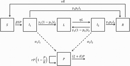A compartmental diagram illustrating the dynamics of salmonellosis among pigs in a pen of a grower-finisher facility is displayed in Figure 1.

Figure 1. Compartmental diagram for Model 1.

Since most grower-finisher pig operations follow an all-in/all-out system of production [18], we assume that the number of pigs in a single pen is constant. That is, $N\left(t\right)=N\left(0\right)=N$ for $t\ge 0$. Therefore, the number of recovered pigs is given by $R\left(t\right)=N-\left(S\right(t)+I_1(t)+L(t)+I_2(t\left)\right)$ and Model 1 can be reduced to a system of five ODEs: (2a) $\frac{\mathrm{d}S}{\mathrm{d}t}=-\beta SP+\nu N-\nu (S+I_1+L+I_2),$(2a) (2b) $\frac{\mathrm{d}{I}_1}{\mathrm{d}t}=\beta SP-{\gamma }_1{I}_1,$(2b) (2c) $\frac{\mathrm{d}L}{\mathrm{d}t}={\gamma }_1(1-p_1)I_1+{\gamma }_2(1-p_2)I_2-\eta L,$(2c) (2d) $\frac{\mathrm{d}{I}_2}{\mathrm{d}t}=\eta L-{\gamma }_2{I}_2,$(2d) (2e) $\frac{\mathrm{d}P}{\mathrm{d}t}={\alpha }_1{I}_1+{\alpha }_2{I}_2+rP(1-\frac{P}{K})-(\xi +\delta )P.$(2e) It is straightforward to verify that all solutions of Equation (2(2a) $\frac{\mathrm{d}S}{\mathrm{d}t}=-\beta SP+\nu N-\nu (S+I_1+L+I_2),$(2a) ) with non-negative initial conditions remain non-negative for all t>0. Moreover, since the pig population size is constant and ${\alpha }_1\ge {\alpha }_2$, it follows from the differential equation for P that (3) $\frac{\mathrm{d}P}{\mathrm{d}t}\le {\alpha }_{1}N-(\xi +\delta -r)P-\frac{r}{K}{P}^2.$(3) Thus, there exists a constant C>0 such that $\underset{t\to \mathrm{\infty }}{lim sup}P\left(t\right)\le C$. The constant C can be taken as the unique positive zero of the quadratic (4) ${\alpha }_{1}N-(\xi +\delta -r)P-\frac{r}{K}{P}^2.$(4) Therefore, the feasible region (5) $\mathrm{\Gamma }=\left\{\right(S,I_1,L,I_2,P)\in {\mathbb{R}}_{+}^5|S+I_1+L+I_2\le N,P\le C\}$(5) is positively invariant with respect to Equation (2(2a) $\frac{\mathrm{d}S}{\mathrm{d}t}=-\beta SP+\nu N-\nu (S+I_1+L+I_2),$(2a) ).

2.2. Basic reproduction number

One of the major goals in modelling epidemics is to determine the risk of infection and develop effective control measures. The basic reproduction number, denoted as ${\mathcal{R}}_0$, is defined as the expected number of secondary infections caused by a typical infectious individual in a completely susceptible population during its infectious period [13,44]. The value of ${\mathcal{R}}_0$ is often used as a threshold for disease persistence or extinction and can be used to quantify the control effort needed to eliminate infection within a population.

In a previous work [18], the authors obtained an expression for the basic reproduction number using the next-generation matrix approach [13,44]. In particular, (6) ${\mathcal{R}}_0=\frac{1}{2}[{\mathcal{R}}_{01}+\sqrt{{\mathcal{R}}_{01}^2+4{\mathcal{R}}_{02}{\mathcal{R}}_{03}}],$(6) where (7) ${\mathcal{R}}_{01}=\frac{r}{\xi +\delta },{\mathcal{R}}_{02}=\frac{\beta N}{\xi +\delta },{\mathcal{R}}_{03}=\frac{{\alpha }_1}{{\gamma }_1}+\frac{{\alpha }_2(1-p_1)}{{\gamma }_2{p}_2}.$(7) The expression for ${\mathcal{R}}_{01}$ can be interpreted as the expected number of secondary CFUs of free-living Salmonella produced by one CFU during its time in the environment through replication. Similarly, ${\mathcal{R}}_{02}$ is the expected number of susceptible pigs infected by one CFU of free-living Salmonella during its time in the environment, and ${\mathcal{R}}_{03}$ is the expected amount of Salmonella shed into the environment by an infected pig during its entire infectious period. For ease of interpretation, note that the units of P and the associated parameters could be rescaled as an infectious dose (the CFU count comprising a median infectious dose) in which case ${\mathcal{R}}_{01}$ could be interpreted as the expected number of secondary infectious doses of free-living Salmonella produced by one infectious dose during its time in the environment. Analogous interpretations hold for ${\mathcal{R}}_{02}$ and ${\mathcal{R}}_{03}$.

Under appropriate environmental conditions, Salmonella is capable of replicating outside of pig hosts [2,18]. It follows directly from Equation (6(6) ${\mathcal{R}}_0=\frac{1}{2}[{\mathcal{R}}_{01}+\sqrt{{\mathcal{R}}_{01}^2+4{\mathcal{R}}_{02}{\mathcal{R}}_{03}}],$(6) ) that ${\mathcal{R}}_0>{\mathcal{R}}_{01}$. Thus, the value of ${\mathcal{R}}_0$ increases with the pathogen growth rate r. If the pathogen can sustain itself in the environment without the need for infected pigs (${\mathcal{R}}_{01}\ge 1$), then ${\mathcal{R}}_0>1$ and it is not possible to eliminate infection from the pen without targeting pathogen growth or increasing the decontamination effort. This suggests that pathogen growth plays a role in the dynamics of salmonellosis in pigs and should be included in models for salmonellosis and other environmentally transmitted infectious diseases.

The following lemma establishes a threshold value which is equivalent to the basic reproduction number. The alternative threshold will be used in the discussion of the stability of the equilibria for Model 1.

Lemma 2.1

For Model 1, ${\mathcal{R}}_0<1$ if and only if (8) ${\mathcal{R}}_{01}+{\mathcal{R}}_{02}{\mathcal{R}}_{03}<1.$(8)

Proof.

By direct calculation, $\begin{array}{rl}\frac{1}{2}[{\mathcal{R}}_{01}+\sqrt{{\mathcal{R}}_{01}^2+4{\mathcal{R}}_{02}{\mathcal{R}}_{03}}]& <1,\\ \sqrt{{\mathcal{R}}_{01}^2+4{\mathcal{R}}_{02}{\mathcal{R}}_{03}}& <2-{\mathcal{R}}_{01},\\ {\mathcal{R}}_{01}^2+4{\mathcal{R}}_{02}{\mathcal{R}}_{03}& <(2-{\mathcal{R}}_{01}{)}^2,\\ 4{\mathcal{R}}_{02}{\mathcal{R}}_{03}& <4-4{\mathcal{R}}_{01},\\ {\mathcal{R}}_{02}{\mathcal{R}}_{03}& <1-{\mathcal{R}}_{01},\\ {\mathcal{R}}_{01}+{\mathcal{R}}_{02}{\mathcal{R}}_{03}& <1.\end{array}$ The above inequalities hold in both directions which completes the proof.

2.3. Equilibria and stability analysis

In this section, we show that ${\mathcal{R}}_0=1$ determines a threshold for the persistence or extinction of salmonellosis in Model 1. In particular, ${\mathcal{R}}_0\le 1$ implies global stability of the unique disease-free equilibrium (DFE) $E_0=(S,I_1,L,I_2,P)=(N,0,0,0,0)$ in the feasible region Γ. That is, salmonellosis disappears from the population. On the other hand, ${\mathcal{R}}_0>1$ implies the existence of a unique endemic equilibrium (EE) and uniform persistence of Model 1. That is, salmonellosis persists within the pig population until the time of slaughter.

The following two theorems establish the local and global stability of the DFE for Model 1, provided that ${\mathcal{R}}_0\le 1$, as well as uniform persistence of Model 1 if ${\mathcal{R}}_0>1$.

Theorem 2.2

For Model 1, the unique DFE is locally asymptotically stable if ${\mathcal{R}}_0<1$ and unstable if ${\mathcal{R}}_0>1$.

Proof.

This theorem follows directly from Theorem 2 of van den Driessche and Watmough [44] since Model 1 satisfies assumptions (A1)–(A5) in [44].

Theorem 2.3

For Model 1,

1. If ${\mathcal{R}}_0\le 1,$ then the DFE is globally asymptotically stable in Γ.

2. If ${\mathcal{R}}_0>1,$ then Model 1 is uniformly persistent.

Proof.

Motivated by Shuai and van den Driessche [41], let $(w_1,w_2,w_3,w_4)=(0,0,0,\beta N)M^{-1},$ where $M=\left[\begin{array}{cccc}{\gamma }_1& 0& 0& 0\\ -{\gamma }_1(1-p_1)& \eta & -{\gamma }_2(1-p_2)& 0\\ 0& -\eta & {\gamma }_2& 0\\ -{\alpha }_1& 0& -{\alpha }_2& \xi +\delta -r\end{array}\right].$ Since $M^{-1}\ge 0$, it follows that $w_j\ge 0$ for $1\le j\le 4$. Notice that if ${\mathcal{R}}_0\le 1$, then ${\mathcal{R}}_{01}<1$ and by Lemma 2.1, $w_1={\mathcal{R}}_{02}{\mathcal{R}}_{03}/(1-{\mathcal{R}}_{01})\le 1$. Construct a Lyapunov function $\mathrm{\Psi }=w_1{I}_1+w_{2}L+w_3{I}_2+w_{4}P.$ Differentiating Ψ along solutions of Equation (2(2a) $\frac{\mathrm{d}S}{\mathrm{d}t}=-\beta SP+\nu N-\nu (S+I_1+L+I_2),$(2a) ), it follows that $\begin{array}{rl}{\mathrm{\Psi }}^{\prime }& ={\frac{\mathrm{d}\mathrm{\Psi }}{\mathrm{d}t}|}_{\left(2\right)}\\ & =w_1(\beta SP-{\gamma }_1{I}_1)+w_2\left({\gamma }_1\right(1-p_1)I_1+{\gamma }_2(1-p_2)I_2-\eta L)\\ & +w_3(\eta L-{\gamma }_2{I}_2)+w_4({\alpha }_1{I}_1+{\alpha }_2{I}_2+rP(1-\frac{P}{K})-(\xi +\delta \left)P\right)\\ & =w_1\beta SP-(w_1{\gamma }_1{I}_1+w_2\eta L+w_3{\gamma }_2{I}_2)\\ & +w_2\left({\gamma }_1\right(1-p_1)I_1+{\gamma }_2(1-p_2\left)I_2\right)+w_3\eta L+w_4({\alpha }_1{I}_1+{\alpha }_2{I}_2)\\ & -w_4\left(\right(\xi +\delta )P-rP(1-\frac{P}{K}))\\ & \le w_1\beta NP-(w_1{\gamma }_1{I}_1+w_2\eta L+w_3{\gamma }_2{I}_2)+w_2\left({\gamma }_1\right(1-p_1)I_1+{\gamma }_2(1-p_2\left)I_2\right)\\ & +w_3\eta L+w_4({\alpha }_1{I}_1+{\alpha }_2{I}_2)-w_4(\xi +\delta -r)P\\ & =w_1(0,0,0,\beta N)(I_1,L,I_2,P{)}^{\mathrm{T}}-(w_1,w_2,w_3,w_4\left)M\right(I_1,L,I_2,P{)}^{\mathrm{T}}\\ & =(w_1-1)\beta NP\le 0.\end{array}$ If ${\mathcal{R}}_0<1$, then ${\mathrm{\Psi }}^{\prime }=0$ implies that $\beta NP=0$. It follows that P=0, and the differential equations for S and $I_1$ are reduced to $S^{\prime }=\nu R$ and $I_1^{\prime }=-{\gamma }_1{I}_1$. Hence, the invariant set where ${\mathrm{\Psi }}^{\prime }=0$ satisfies $I_1=R=0$. It follows from the differential equation for R that the invariant set where ${\mathrm{\Psi }}^{\prime }=0$ satisfies $I_2=0$. Using the differential equation for L, the invariant set where ${\mathrm{\Psi }}^{\prime }=0$ satisfies L=0. Since the pig population size is constant, S=N, and the largest invariant set where ${\mathrm{\Psi }}^{\prime }=0$ is the singleton $\left\{E_0\right\}$. By LaSalle's Invariance Principle [26], $E_0$ is globally asymptotically stable in Γ if ${\mathcal{R}}_0<1$.

If ${\mathcal{R}}_0=1$, then ${\mathrm{\Psi }}^{\prime }=0$ implies that $\beta SP=\beta NP$ and $\left(r/K\right)P^2=0$. If r=0, then S=N and if $r\ne 0$, then P=0. In either case, it follows that the largest invariant set for which ${\mathrm{\Psi }}^{\prime }=0$ is the singleton $\left\{E_0\right\}$. By LaSalle's Invariance Principle, $E_0$ is globally asymptotically stable in Γ if ${\mathcal{R}}_0=1$.

If ${\mathcal{R}}_0>1$, then by continuity, ${\mathrm{\Psi }}^{\prime }>0$ in a neighbourhood of $E_0$ in $\stackrel{\circ }{\mathrm{\Gamma }}$. Solutions in $\stackrel{\circ }{\mathrm{\Gamma }}$ sufficiently close to $E_0$ move away from $E_0$, implying that $E_0$ is unstable. Using a uniform persistence result from [15] and an argument as in the proof of Proposition 3.3 of Li et al. [28], it can be shown that, when ${\mathcal{R}}_0>1$, instability of $E_0$ implies uniform persistence of the model.

The following theorem establishes that ${\mathcal{R}}_0>1$ is a necessary and sufficient condition for the existence of a unique EE.

Theorem 2.4

Model 1 admits a unique EE if and only if ${\mathcal{R}}_0>1$.

Proof.

The equilibrium equations for Model 1 are $\begin{array}{rl}\beta SP& =\nu R,\\ \beta SP& ={\gamma }_1{I}_1,\\ \eta L& ={\gamma }_1(1-p_1)I_1+{\gamma }_2(1-p_2)I_2,\\ \eta L& ={\gamma }_2{I}_2,\\ {\gamma }_1{p}_1{I}_1+{\gamma }_2{p}_2{I}_2& =\nu R,\\ {\alpha }_1{I}_1+{\alpha }_2{I}_2+rP(1-\frac{P}{K})& =(\xi +\delta )P.\end{array}$ It follows that an EE must satisfy $\begin{array}{rl}{I}_1=\psi \left(P\right)& =\frac{{\gamma }_2{p}_2}{{\alpha }_1{\gamma }_2{p}_2+{\alpha }_2{\gamma }_1(1-p_1)}[\frac{r}{K}{P}^2+(\xi +\delta -r\left)P\right],\\ P=\phi \left(I_1\right)& =\frac{{\gamma }_1{I}_1}{\beta [N-I_1(1+\frac{{\gamma }_1(1-p_1)}{\eta p_2}+\frac{{\gamma }_1(1-p_1)}{{\gamma }_2{p}_2}+\frac{{\gamma }_1}{\nu })]}.\end{array}$ An EE exists if and only if the graphs of $I_1=\psi \left(P\right)$ and $P=\phi \left(I_1\right)$ intersect in ${\mathbb{R}}_{+}^2$. There exists at most one intersection of the graphs of $P=\phi \left(I_1\right)$ and $I_1=\psi \left(P\right)$, and thus there is at most one EE (see Figure 2). If ${\mathcal{R}}_{01}\ge 1$, then ${\mathcal{R}}_0>1$ and an intersection always exists. On the other hand, if ${\mathcal{R}}_{01}<1$, then the curves intersect if and only if ${\psi }^{\prime }\left(0\right)<1/{\phi }^{\prime }\left(0\right)$. That is, $\begin{array}{rl}& \frac{{\gamma }_2{p}_2(\xi +\delta -r)}{{\alpha }_1{\gamma }_2{p}_2+{\alpha }_2{\gamma }_1(1-p_1)}<\frac{\beta N}{{\gamma }_1}\\ & \frac{{\gamma }_2{p}_2(1-{\mathcal{R}}_{01})}{{\alpha }_1{\gamma }_2{p}_2+{\alpha }_2{\gamma }_1(1-p_1)}<\frac{\beta N}{{\gamma }_1(\xi +\delta )}\\ & {\gamma }_2{p}_2(1-{\mathcal{R}}_{01})<\frac{\beta N}{\xi +\delta }[\frac{{\alpha }_1{\gamma }_2{p}_2}{{\gamma }_1}+{\alpha }_2(1-p_1\left)\right]\\ & 1-{\mathcal{R}}_{01}<{\mathcal{R}}_{02}{\mathcal{R}}_{03}\\ & 1<{\mathcal{R}}_{01}+{\mathcal{R}}_{02}{\mathcal{R}}_{03}.\end{array}$ By Lemma 2.1, the necessary and sufficient condition for the existence of a unique EE is ${\mathcal{R}}_0>1$.

Figure 2. Graphs of the functions $P=\phi \left(I_1\right)$ and $I_1=\psi \left(P\right)$ for ${\mathcal{R}}_{01}<1$ and ${\mathcal{R}}_0>1$.

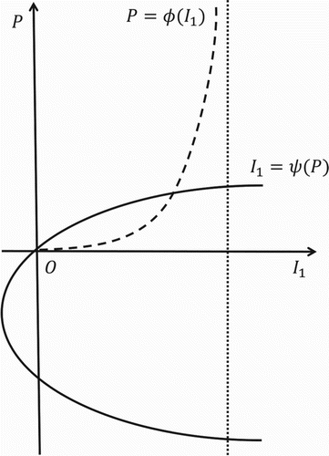
For Model 1, the local or global stability of the EE has not been established and is currently an open problem. However, it should be noted that stability of the EE is a long-term result and for salmonellosis in pigs in a pen of a grower-finisher facility, the primary interest is the prevalence of infection at slaughter rather than long-term prevalence. Numerical simulations of Model 1 suggest that if ${\mathcal{R}}_0>1$, then the EE is globally asymptotically stable in $\mathrm{int}\left(\mathrm{\Gamma }\right)$, but pigs are sold for slaughter prior to the solution stabilizing at the EE. Establishing the local or global stability of the EE for Model 1 would be of theoretical interest, but it is not necessary for our objectives in this manuscript.

2.4. Control measures

In Section 2.3, we established that the basic reproduction number serves as a threshold for the long-term persistence or extinction of salmonellosis among pigs in a pen of a grower-finisher facility. If ${\mathcal{R}}_0\le 1$, then salmonellosis is eradicated from the population and if ${\mathcal{R}}_0>1$, then Model 1 is uniformly persistent and the infection persists until the pigs are sold for slaughter. To eradicate salmonellosis infection in pigs in a pen of a grower-finisher operation, control measures must be implemented so that the value of ${\mathcal{R}}_0$ is less than or equal to one. Possible control methods include improved environmental decontamination (increase δ), vaccination of pigs (decrease ${\alpha }_i$ and/or increase ${\gamma }_i$), and isolation of infected pigs to decrease the probability of contact with free-living Salmonella (decrease β). The expression for ${\mathcal{R}}_0$ in Equation (6(6) ${\mathcal{R}}_0=\frac{1}{2}[{\mathcal{R}}_{01}+\sqrt{{\mathcal{R}}_{01}^2+4{\mathcal{R}}_{02}{\mathcal{R}}_{03}}],$(6) ) can be used to quantify the minimum control effort needed for disease eradication. For this system, control efforts can be applied to either the pig population, free-living Salmonella, or both. 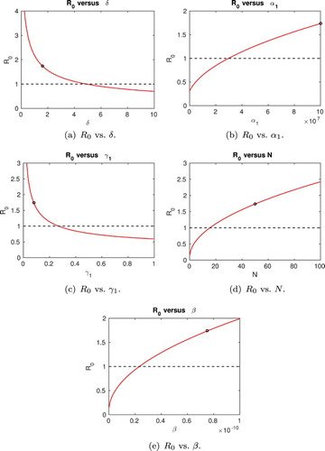To determine the efficacy of different control measures, we consider ${\mathcal{R}}_0$ as a function of the model parameters and plot ${\mathcal{R}}_0$ over a range of feasible parameter values as in [30]. Variations in certain parameter values are not considered due to the fact that such control measures are not reasonable or are insufficient to eradicate salmonellosis.

We begin by considering the parameter values presented in [18,22], summarized in Table 1, which describe the transmission of Salmonella Typhimurium infection among pigs in a pen of a grower-finisher facility. For the parameter values in Table 1, the basic reproduction number is ${\mathcal{R}}_0=1.74$. Since ${\mathcal{R}}_0>1$, there exists a unique EE for Model 1 given by $E^{\ast }=(S^{\ast },I_1^{\ast },L^{\ast },I_2^{\ast },R^{\ast },P^{\ast })=(15.5,2.6,6.0,4.9,20.9,1.8\times {10}^8).$ A simple calculation shows that the eigenvalues of the Jacobian matrix at $E^{\ast }$ have negative real parts. Therefore, the EE is locally asymptotically stable for the parameter values in Table 1.

Table 1. Parameter values for salmonellosis among pigs.

Parameter	Definition	Value	Ref.
β	Indirect transmission rate	$7.5\times {10}^{-11}$	[18]
${\gamma }_1$	Recovery rate from $I_1$	0.08	[18,22]
${\gamma }_2$	Recovery rate from $I_2$	0.303	[18,22]
$p_1$	Fraction of $I_1$ recovering	0.07	[18,22]
$p_2$	Fraction of $I_2$ recovering	0.13	[18,22]
$1/\eta$	Duration of latent period	4	[18,22]
ν	Loss of immunity rate	0.01	[18,22]
${\alpha }_1$	Shedding rate for $I_1$	${10}^8$	[18]
${\alpha }_2$	Shedding rate for $I_2$	${10}^6$	[18]
r	FLP growth rate	0.25	[18]
K	FLP carrying capacity	$3.33\times {10}^{10}$	[18]
ξ	FLP death rate	0.12	[18]
δ	Decontamination rate	1.61	[18]

A common method for preventing the transmission of salmonellosis among pigs in a pen of a grower-finisher facility is the removal of contaminated fecal waste via environmental decontamination [18]. The methods and efficacy of decontamination vary across facilities [18]. Bani-Yaghoub et al. established an equation relating the decontamination rate to the proportion of free-living Salmonella removed from the environment each day [3]. The relationship is given by (9) $P_{\mathrm{Removed}}=(1-{\mathrm{e}}^{-\delta })\times 100.$(9) To determine the efficacy of environmental decontamination, we consider the change in the basic reproduction number for Model 1 as the decontamination rate varies over the feasible range $0\le \delta \le 10$. Thus, the range of values $0\le \delta \le 10$ corresponds to a daily pathogen removal efficacy of 0–99.99 % .

Vaccination of pigs is not commonly used in practice, but could be implemented as a control method in grower-finisher facilities [10,12,36,39]. In recent years, vaccines have been developed to reduce the shedding rate of infected pigs (${\alpha }_i$, i=1,2) and/or decrease the duration of infection ($1/{\gamma }_i$, i=1,2) [10]. Although it is unlikely that a specific subgroup of infected pigs would be vaccinated (e.g. $I_1$ vs. $I_2$), our results suggest that vaccination of pigs in the early stage of infection ($I_1$) is more effective than vaccination of pigs in later stages of infection ($I_2$). Indeed, (10) $\underset{{\alpha }_2\to 0^{+}}{lim}{\mathcal{R}}_{03}=\underset{{\gamma }_2\to \mathrm{\infty }}{lim}{\mathcal{R}}_{03}=\frac{{\alpha }_1}{{\gamma }_1}.$(10) For the parameter values in Table 1, ${\alpha }_1/{\gamma }_1>1$. Thus, salmonellosis cannot be eradicated by only vaccinating pigs in state $I_2$. Therefore, we consider the change in the basic reproduction number for varying ${\alpha }_1$ and ${\gamma }_1$, but not for variations in ${\alpha }_2$ or ${\gamma }_2$. The feasible range of values for ${\alpha }_1$ is taken as $0\le {\alpha }_1\le {10}^8$, whereas the range of values for ${\gamma }_1$ is $0<{\gamma }_1\le 1$.

Additional control measures can be used to target the force of infection corresponding to indirect transmission. Examples include reducing the total number of pigs in each pen, N, or using probiotics to decrease the probability of infection when a susceptible pig ingests free-living Salmonella (reduce β) [9]. We assume that the feasible range of values for N is $0<N\le 100$, whereas the range of values for β is $0\le \beta \le {10}^{-10}$.

In Figure 3, variations of the basic reproduction number are plotted as each of the parameter values is varied over its feasible range while all other parameter values are kept at their constant baseline values in Table 1.

Figure 3. The basic reproduction number, ${\mathcal{R}}_0$, plotted against varying parameter values. In each case, a single parameter is varied and all other parameter values are as in Table 1. The point plotted on each curve represents the value of ${\mathcal{R}}_0$ for the baseline parameter values in Table 1. The dashed line ${\mathcal{R}}_0=1$ indicates the threshold for persistence or disappearance of the infection.

3. Model with continuous shedding (Model 2)

3.1. Model development

In Section 2, a model was developed for salmonellosis in pigs in a pen of a grower-finisher facility. Model 1 accounts for intermittent infectiousness explicitly by allowing infected pigs to cycle through stages of active shedding and non-shedding throughout their infected period. In this section, a simplified modelling approach is considered for which intermittent infectiousness is neglected and infected pigs are assumed to shed Salmonella into the environment continuously during their infected period.

At the time of slaughter, pork products can be contaminated by Salmonella in the digestive tract of an infected pig. Therefore, our primary interest is the total number of infected pigs at the time of slaughter, $I_1+L+I_2$, rather than the number of pigs in each infected group. Thus, the three infected groups ($I_1$, L and $I_2$) from Model 1 could be reduced to one infected state $I=I_1+L+I_2$ which represents infected pigs.

Model 2 divides the pig population into three groups based on infection status: susceptible (S), infected (I), or recovered (R). It is assumed that infected pigs shed Salmonella into the environment continuously at an average rate of $\overline{\alpha }>0$ CFU/day for an average duration of $1/\overline{\gamma }$ days, where $\overline{\gamma }>0$. The parameters used in Model 2 are the same as in Model 1, with the exception of the average shedding rate $\overline{\alpha }$ and the average recovery rate $\overline{\gamma }$.

Model 2 is defined by the following system of ODEs: (11a) $\frac{\mathrm{d}S}{\mathrm{d}t}=-\beta SP+\nu R,$(11a) (11b) $\frac{\mathrm{d}I}{\mathrm{d}t}=\beta SP-\overline{\gamma }I,$(11b) (11c) $\frac{\mathrm{d}R}{\mathrm{d}t}=\overline{\gamma }I-\nu R,$(11c) (11d) $\frac{\mathrm{d}P}{\mathrm{d}t}=\overline{\alpha }I+rP(1-\frac{P}{K})-(\xi +\delta )P.$(11d) A compartmental diagram illustrating the dynamics of salmonellosis among pigs in a pen of a grower-finisher facility is displayed in Figure 4.

Figure 4. Compartmental diagram for Model 2.

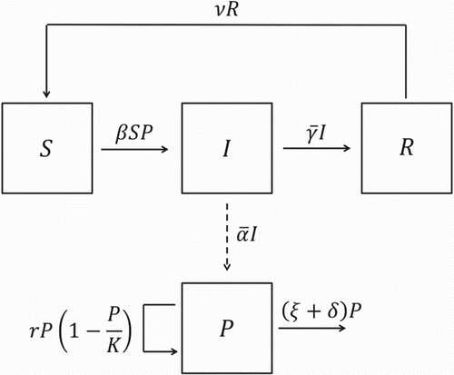
As in Model 1, the total number of pigs is assumed to be constant, as justified by the use of an all-in/all-out system of production and no mortality [18]. Therefore, the number of recovered pigs is given by $R=N-(S+I)$ and Model 2 can be reduced to a three-dimensional system: (12a) $\frac{\mathrm{d}S}{\mathrm{d}t}=-\beta SP+\nu N-\nu (S+I),$(12a) (12b) $\frac{\mathrm{d}I}{\mathrm{d}t}=\beta SP-\overline{\gamma }I,$(12b) (12c) $\frac{\mathrm{d}P}{\mathrm{d}t}=\overline{\alpha }I+rP(1-\frac{P}{K})-(\xi +\delta )P.$(12c)

To compute the average shedding and recovery rates, $\overline{\alpha }$ and $\overline{\gamma }$, we must consider the average amount of time a pig spends in each infected state over the course of its infected period. As discussed in Section 2.2, once a susceptible pig becomes infected it will spend an average of ${\tau }_1=1/{\gamma }_1$ days in state $I_1$, ${\tau }_{\ell }=(1-p_1)/\eta p_2$ days in state L, and ${\tau }_2=(1-p_1)/{\gamma }_2{p}_2$ days in state $I_2$ over the entire course of its infected period. Therefore, an infected pig is actively shedding for an average of ${\tau }_1+{\tau }_2$ days during its average infected period of ${\tau }_1+{\tau }_{\ell }+{\tau }_2$ days. Thus, the average recovery rate could be calculated as (13) $\overline{{\gamma }_I}=\frac{1}{{\tau }_1+{\tau }_2}\text{or}\overline{{\gamma }_{II}}=\frac{1}{{\tau }_1+{\tau }_{\ell }+{\tau }_2}.$(13) Similarly, the average shedding rate could be calculated as (14) $\overline{{\alpha }_I}=\frac{{\alpha }_1{\tau }_1+{\alpha }_2{\tau }_2}{{\tau }_1+{\tau }_2}\text{or}\overline{{\alpha }_{II}}=\frac{{\alpha }_1{\tau }_1+{\alpha }_2{\tau }_2}{{\tau }_1+{\tau }_{\ell }+{\tau }_2}.$(14) These values could be computed by collecting epidemiological data by repeatedly sampling the same animals throughout their infected period [22] . The average duration of infection is estimated as either the duration of observed shedding, ($\overline{{\gamma }_I}$) or the difference from the last to the first day of observed shedding ($\overline{{\gamma }_{II}}$). Similarly, the average shedding rate is calculated as an average of observed shedding rates ($\overline{{\alpha }_I}$) or the average shedding rate from the first day to the last day of observed shedding ($\overline{{\alpha }_{II}}$).

Each of these expressions represents a reasonable and intuitive way to compute the average shedding and recovery rates. However, with two approaches for estimation of each of the two parameters, there are four combinations (cases) to consider for Model 2:

1. The average shedding rate is $\overline{{\alpha }_I}$ and the average recovery rate is $\overline{{\gamma }_I}$.

2. The average shedding rate is $\overline{{\alpha }_{II}}$ and the average recovery rate is $\overline{{\gamma }_{II}}$.

3. The average shedding rate is $\overline{{\alpha }_I}$ and the average recovery rate is $\overline{{\gamma }_{II}}$.

4. The average shedding rate is $\overline{{\alpha }_{II}}$ and the average recovery rate is $\overline{{\gamma }_I}$.

3.2. Basic reproduction number

An expression for the basic reproduction number is obtained using the next-generation matrix approach. The Jacobian matrix for the infected groups (I and P) evaluated at the unique DFE is (15) $J=\left[\begin{array}{cc}-\overline{\gamma }& \beta N\\ \overline{\alpha }& r-(\xi +\delta )\end{array}\right]=\left[\begin{array}{cc}0& \beta N\\ \overline{\alpha }& r\end{array}\right]-\left[\begin{array}{cc}\overline{\gamma }& 0\\ 0& \xi +\delta \end{array}\right]=F-V.$(15) Therefore, the next-generation matrix is (16) $F{V}^{-1}=\left[\begin{array}{cc}0& \frac{\beta N}{\xi +\delta }\\ \frac{\overline{\alpha }}{\overline{\gamma }}& \frac{r}{\xi +\delta }\end{array}\right].$(16) The basic reproduction number for Model 2 is given by (17) ${\overline{\mathcal{R}}}_0=\frac{1}{2}[{\mathcal{R}}_{01}+\sqrt{{\mathcal{R}}_{01}^2+4{\mathcal{R}}_{02}\left(\frac{\overline{\alpha }}{\overline{\gamma }}\right)}],$(17) where ${\mathcal{R}}_{01}$ and ${\mathcal{R}}_{02}$ are as in Equation (7(7) ${\mathcal{R}}_{01}=\frac{r}{\xi +\delta },{\mathcal{R}}_{02}=\frac{\beta N}{\xi +\delta },{\mathcal{R}}_{03}=\frac{{\alpha }_1}{{\gamma }_1}+\frac{{\alpha }_2(1-p_1)}{{\gamma }_2{p}_2}.$(7) ). The term $\overline{\alpha }/\overline{\gamma }$ represents the average amount of Salmonella shed by an infected pig during its infected period. To distinguish between the value of ${\overline{\mathcal{R}}}_0$ for cases (a)–(d), we denote the basic reproduction number for case (a) by ${\overline{\mathcal{R}}}_{0a}$. Similar notation is used for cases (b)–(d).

Since Model 1 can be reduced to Model 2 by setting $p_1=1$, ${\alpha }_1=\overline{\alpha }$, and ${\gamma }_1=\overline{\gamma }$, the results established in Theorems 2.2–2.4 of Section 2.3 hold for both Model 1 and Model 2. In particular, salmonellosis disappears from the pig population if ${\overline{\mathcal{R}}}_0\le 1$ and persists within the population if ${\overline{\mathcal{R}}}_0>1$. However, using different methods to compute the average shedding and recovery rates, as in cases (a)–(d), may result in different values for the basic reproduction number.

Theorem 3.1

The basic reproduction numbers, ${\mathcal{R}}_0$ and ${\overline{\mathcal{R}}}_0,$ satisfy the following:

1. ${\overline{\mathcal{R}}}_{0a}={\overline{\mathcal{R}}}_{0b}={\mathcal{R}}_0,$

2. ${\overline{\mathcal{R}}}_{0c}\ge {\mathcal{R}}_0,$

3. ${\overline{\mathcal{R}}}_{0d}\le {\mathcal{R}}_0$.

Proof.

For cases (a) and (b), it follows that (18) $\frac{\overline{{\alpha }_I}}{\overline{{\gamma }_I}}=\frac{\overline{{\alpha }_{II}}}{\overline{{\gamma }_{II}}}={\alpha }_1{\tau }_1+{\alpha }_2{\tau }_2={\mathcal{R}}_{03},$(18) where ${\mathcal{R}}_{03}$ is as in Equation (7(7) ${\mathcal{R}}_{01}=\frac{r}{\xi +\delta },{\mathcal{R}}_{02}=\frac{\beta N}{\xi +\delta },{\mathcal{R}}_{03}=\frac{{\alpha }_1}{{\gamma }_1}+\frac{{\alpha }_2(1-p_1)}{{\gamma }_2{p}_2}.$(7) ). Therefore, (19) ${\overline{\mathcal{R}}}_{0a}={\overline{\mathcal{R}}}_{0b}=\frac{1}{2}[{\mathcal{R}}_{01}+\sqrt{{\mathcal{R}}_{01}^2+4{\mathcal{R}}_{02}{\mathcal{R}}_{03}}]={\mathcal{R}}_0.$(19) For cases (c) and (d), it follows that (20) $\begin{array}{rl}\frac{\overline{{\alpha }_I}}{\overline{{\gamma }_{II}}}& =({\alpha }_1{\tau }_1+{\alpha }_2{\tau }_2)\left(\frac{{\tau }_1+{\tau }_{\ell }+{\tau }_2}{{\tau }_1+{\tau }_2}\right)\ge {\mathcal{R}}_{03},\\ \frac{\overline{{\alpha }_{II}}}{\overline{{\gamma }_I}}& =({\alpha }_1{\tau }_1+{\alpha }_2{\tau }_2)\left(\frac{{\tau }_1+{\tau }_2}{{\tau }_1+{\tau }_{\ell }+{\tau }_2}\right)\le {\mathcal{R}}_{03}.\end{array}$(20) Therefore, (21) $\begin{array}{rl}{\overline{\mathcal{R}}}_{0c}& \ge \frac{1}{2}[{\mathcal{R}}_{01}+\sqrt{{\mathcal{R}}_{01}^2+4{\mathcal{R}}_{02}{\mathcal{R}}_{03}}]={\mathcal{R}}_0\\ {\overline{\mathcal{R}}}_{0d}& \le \frac{1}{2}[{\mathcal{R}}_{01}+\sqrt{{\mathcal{R}}_{01}^2+4{\mathcal{R}}_{02}{\mathcal{R}}_{03}}]={\mathcal{R}}_0.\end{array}$(21)

For cases (a) and (b) of Model 2, ${\mathcal{R}}_0={\overline{\mathcal{R}}}_0$. That is, the two modelling assumptions regarding intermittent shedding yield the same value for the basic reproduction number provided that the average shedding and recovery rates are calculated as in cases (a) and (b). For Model 2 case (c), the average length of infection includes ${\tau }_{\ell }$ which is not included in the average shedding rate. Therefore, shedding occurs for a longer period of time than would be expected for the shedding rate ${\overline{\alpha }}_I$ and we obtain a larger value for the basic reproduction number (${\overline{\mathcal{R}}}_{0c}\ge {\mathcal{R}}_0$). For Model 2 case (d), the average length of infection does not include ${\tau }_{\ell }$ which is included in the average shedding rate. Therefore, shedding occurs for a shorter period of time than would be expected for the shedding rate ${\overline{\alpha }}_{II}$ and we obtain a smaller value for the basic reproduction number (${\overline{\mathcal{R}}}_{0d}\le {\mathcal{R}}_0$). Thus, case (c) may yield an overestimate for the basic reproduction number resulting in economic losses or wasted resources due to an unnecessarily extensive control. On the other hand, case (d) may yield an underestimate for the reproduction number leading to control efforts which are insufficient for disease eradication or additional cases of human infection and/or death.

In the next section, we compare numerical simulations for Models 1 and 2 using the parameter values from [18,22] to evaluate the role of intermittent fecal shedding in the transmission of salmonellosis among pigs in a pen of a grower-finisher facility.

4. Numerical simulation of models 1 and 2

The dynamics of salmonellosis among pigs in a pen of an all-in/all-out grower-finisher facility are illustrated through several numerical examples. In the first set of examples, we consider the slaughter-age prevalence of infection under the modelling assumptions of intermittent and continuous shedding. In the second set of examples, we consider the impact of intermittent shedding on disease control strategies for salmonellosis in a pen of grower-finisher pigs.

4.1. Prevalence of infection

In a grower-finisher facility, pigs are sold for slaughter after an average of 150 days [18,22]. At the time of slaughter, pork products can be contaminated from Salmonella in the gut of an infected pig. Therefore, we are particularly interested in the prevalence of infection, $\left[I_1\right(t)+L(t)+I_2(t\left)\right]/N$, at t=150 days. To determine the effects of intermittent shedding on slaughter-age prevalence, we perform numerical simulations of Model 1 and Model 2 using the parameter values from [18,22] summarized in Table 1, which describe transmission of Salmonella Typhimurium infection among pigs in a pen of a grower-finisher facility.

Using the parameter values in Table 1, the average shedding and recovery rates for Model 2 can be computed using the methods discussed in Section 3. The average shedding rate is given by $\overline{{\alpha }_I}=3.53\times {10}^7$ or $\overline{{\alpha }_{II}}=1.97\times {10}^7$, while the average recovery rate is given by $\overline{{\gamma }_I}=0.0277$ or $\overline{{\gamma }_{II}}=0.0154$. It follows that the basic reproduction numbers for Model 2 cases (a)–(d) are ${\overline{\mathcal{R}}}_{0a}={\overline{\mathcal{R}}}_{0b}={\mathcal{R}}_0=1.74$, ${\overline{\mathcal{R}}}_{0c}=2.3$, and ${\overline{\mathcal{R}}}_{0d}=1.32$. As discussed in Section 3, neglecting the intermittent shedding pattern can lead to different expressions for the basic reproduction number depending on how the average shedding and recovery rates are computed. The implications for disease control are discussed in Section 4.2.

Figure 5 illustrates the simulated prevalence of infection for Model 1, $(I_1+L+I_2)/N$, along with the simulated prevalence for Model 2 (cases (a)–(d)), I/N. The numerical simulation of Model 1 shown in Figure 5 illustrates a large initial peak in infection prevalence followed by dampened oscillations before stabilization at an endemic level of $27.1\mathrm{\%}$. At the average slaughter age, infection prevalence is $18.5\mathrm{\%}$. It should be noted that stabilization at the unique EE for Model 1 does not occur until after the time of slaughter.

Figure 5. Prevalence of salmonellosis infection among N=50 pigs in a pen of a grower-finisher facility illustrating an outbreak and disease persistence. Parameter values are as in Table 1 with initial conditions $S\left(0\right)=49$, $I_1\left(0\right)=1$, $L\left(0\right)=0$, $I_2\left(0\right)=0$, $R\left(0\right)=0$, and $P\left(0\right)=0$. The results for Model 1 and Model 2 cases (a)–(d) are plotted over time. The basic reproduction numbers for Models 1 and 2 are given by ${\overline{\mathcal{R}}}_{0a}={\overline{\mathcal{R}}}_{0b}={\mathcal{R}}_0=1.74$, ${\overline{\mathcal{R}}}_{0c}=2.3$, and ${\overline{\mathcal{R}}}_{0d}=1.32$, respectively. At the average slaughter age, t=150, the prevalence of infection is 18.5% (Model 1), 22.5% (Model 2a), 38.0% (Model 2b), 39.1% (Model 2c), and 15.2% (Model 2d).

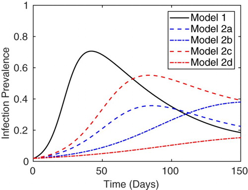
For the simulation of Model 2 shown in Figure 5, there is an initial peak in prevalence followed by stabilization at some endemic level. In each of the cases (a)–(d), the initial outbreak occurs at a lower level than Model 1. The long-term and slaughter-age prevalence of infection depend on the method used to compute the average shedding and recovery rate. In particular, the slaughter-age prevalence of infection for Model 2 cases (a), (b), and (c) are 22.5%, 38.0%, and 39.1%, respectively. For cases (a)–(c), the simulated slaughter-age prevalence is larger than the simulated prevalence for Model 1. On the other hand, Model 2 case (d) yields a slaughter-age prevalence of 15.2%, which is a lower prevalence than Model 1. Although the slaughter-age prevalence in cases (a) and (d) are relatively close to the simulated prevalence for Model 1, there are significant differences in the size of the initial outbreak as well as the long-term prevalence of infection. Cases (c) and (d) of Model 2 result in the largest and smallest slaughter-age prevalences, respectively. These results are consistent with what we might intuitively expect since Model 2 case (c) includes the latent period ${\tau }_{\ell }$ in the average length of infection, but not the average shedding rate (${\mathcal{R}}_{0c}\ge {\mathcal{R}}_0$), whereas Model 2 case (d) includes ${\tau }_{\ell }$ in the average shedding rate, but not the average length of infection (${\mathcal{R}}_{0d}\le {\mathcal{R}}_0$). The differences between Model 1 and Model 2 cases (a)–(d) illustrated in Figure 5 remained valid for numerical simulations of the two models performed for other sets of parameter values for which ${\mathcal{R}}_0>1$. In particular, the initial peak in simulated prevalance for Model 1 was consistently larger than the peak prevalance for all cases of Model 2 and cases (c) or (d) of Model 2 always resulted in the largest or smallest long-term prevalence of infection, respectively.

In Figure 6, we compare the simulated shedding prevalence for Model 1, $(I_1+I_2)/N$, and Model 2 cases (a)–(d), I/N, using the parameter values from Table 1 with epidemiological data taken from [17,18]. By inspection of the figure, it is clear that the simulated shedding prevalence for Model 1 is a better fit to the data than simulations for Model 2.

Figure 6. Simulated shedding prevalence among N=50 pigs in a pen of a grower-finisher facility and epidemiological data taken from [17,18]. Parameter values are as in Table 1 with initial conditions $S\left(0\right)=49$, $I_1\left(0\right)=1$, $L\left(0\right)=0$, $I_2\left(0\right)=0$, $R\left(0\right)=0$, and $P\left(0\right)=0$. Note that simulations of Model 1 yield the best fit for the data.

In this subsection, we have established that neglecting the intermittent shedding pattern of infected pigs can result in different values for the basic reproduction number as well as the slaughter-age or long-term prevalence of infection, depending on how the average shedding and recovery rates are computed. The drastic differences between Model 1 and Model 2 cases (c)–(d) demonstrate that neglecting intermittent shedding may cause modelling inaccuracies. In the next subsection, we explore the effects of intermittent shedding on the development of infection control strategies.

4.2. Impacts on control

In Section 2.3, we established that the basic reproduction number serves as a threshold for disease persistence or extinction. In particular, it follows from Theorem 2.3 that Salmonella infection can be eliminated from a pen of pigs by ensuring ${\mathcal{R}}_0\le 1$. Therefore, the expression for ${\mathcal{R}}_0$ in Equation (6(6) ${\mathcal{R}}_0=\frac{1}{2}[{\mathcal{R}}_{01}+\sqrt{{\mathcal{R}}_{01}^2+4{\mathcal{R}}_{02}{\mathcal{R}}_{03}}],$(6) ) can be used to quantify the amount of control needed to reduce or eliminate infection within a pen [1,13]. The minimal efficacy needed to drive the disease to extinction can be quantified for various control strategies by setting ${\mathcal{R}}_0=1$.

In Section 3.2, we found that Model 1 and Model 2 may result in different expressions for the basic reproduction number (i.e. ${\mathcal{R}}_0$ vs. ${\overline{\mathcal{R}}}_0$) depending on how the average shedding and recovery rates for Model 2 are calculated. Calculating the average rates as in case (c) may result in an overestimate for the basic reproduction number, whereas case (d) may result in an underestimate for ${\mathcal{R}}_0$. In this subsection, we consider the impacts of different modelling assumptions regarding intermittent shedding on infection control.

Recall from Section 2.4 that there are a considerable number of control strategies available for salmonellosis in pigs in a pen of a grower-finisher facility. These controls include environmental decontamination/cleaning, vaccination of infected pigs to reduce their shedding rate and/or duration of infection, decreasing the number of pigs in each pen, and use of probiotics to decrease the risk of infection when a susceptible pig ingests free-living Salmonella from the environment [9,10,18]. In Figure 7, we illustrate the changes in the basic reproduction numbers for Models 1 and 2 (${\mathcal{R}}_0$ and ${\overline{\mathcal{R}}}_0$) for varying levels of control.

Figure 7. The effect of various control efforts on the basic reproduction number. Reproduction numbers are plotted for both Model 1 (${\mathcal{R}}_0$) and Model 2 cases (c) and (d) (${\overline{\mathcal{R}}}_{0c}$ and ${\overline{\mathcal{R}}}_{0d}$). For cases (a) and (b), the value of ${\overline{\mathcal{R}}}_0$ is equal to that of ${\mathcal{R}}_0$. The dashed horizontal line ${\mathcal{R}}_0=1$ corresponds to the threshold for long-term disease persistence or extinction. Parameter values are as in Table 1, with the exception of the individual parameter being varied in each case.

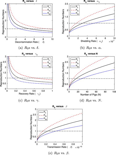
Let us begin by considering environmental decontamination/cleaning of pens. In order to eliminate salmonellosis from the pen (${\mathcal{R}}_0\le 1$), it is necessary to increase the decontamination rate such that $\delta \ge 4.91$. On the other hand, a value of $\delta \ge 8.7$ is required to ensure ${\overline{\mathcal{R}}}_{0c}\le 1$ while $\delta \ge 2.8$ is sufficient for ${\overline{\mathcal{R}}}_{0d}\le 1$. Using Equation (9(9) $P_{\mathrm{Removed}}=(1-{\mathrm{e}}^{-\delta })\times 100.$(9) ), we find that the value $\delta =4.91$ corresponds to cleaning the pen once daily with a pathogen removal efficacy of approximately $99\mathrm{\%}$, while $\delta =8.7$ and $\delta =2.8$ correspond to a removal efficacy of approximately $100\mathrm{\%}$ and $94\mathrm{\%}$, respectively. Either of these levels of pathogen removal may not be feasible in practice, indicating that environmental decontamination alone is not an effective control for salmonellosis. These findings are consistent with the authors' previous results [18].

Next, we consider vaccination of pigs to reduce their shedding level and/or duration of infection. As in Section 2.4, we only consider vaccination of pigs in the first stage of infection ($I_1$) since targeting pigs only in the later stages of infection (L and $I_2$) is insufficient to eliminate salmonellosis from the pen. In order to ensure that ${\mathcal{R}}_0\le 1$, the shedding rate ${\alpha }_1$ must be reduced so that ${\alpha }_1\le 2.96\times {10}^7$. In contrast, an increased reduction of ${\alpha }_1\le 1.57\times {10}^7$ is required so that ${\overline{\mathcal{R}}}_{0c}\le 1$, while a smaller reduction in the shedding rate ${\alpha }_1\le 5.47\times {10}^7$ is sufficient for ${\overline{\mathcal{R}}}_{0d}\le 1$. Similarly, the duration of the first stage of infection $1/{\gamma }_1$ must be increased so that ${\gamma }_1\ge 0.27$ to ensure ${\mathcal{R}}_0\le 1$ while ${\gamma }_1\ge 0.63$ is required for ${\overline{\mathcal{R}}}_{0c}\le 1$ and ${\gamma }_1\ge 0.14$ is sufficient for ${\overline{\mathcal{R}}}_{0d}\le 1$.

Last, we consider controls which decrease the force of infection due to indirect transmission. If fewer pigs are raised in each pen, the risk of an outbreak is decreased. To eliminate salmonellosis from the pen, the number of pigs must be reduced so that ${\mathcal{R}}_0\le 1$. That is, the population in each pen must be $N\le 15$. Alternatively, a population of $N\le 8$ is necessary for ${\overline{\mathcal{R}}}_{0c}\le 1$ while $N\le 27$ will ensure ${\overline{\mathcal{R}}}_{0d}\le 1$. Similarly, if probiotics are used to decrease the risk of infection for susceptible pigs, then the transmission parameter β can be reduced. In order to eliminate salmonellosis in the pen (${\mathcal{R}}_0\le 1$), the transmission parameter must be reduced so that $\beta \le 2.3\times {10}^{-11}$. However, a value of $\beta \le 1.3\times {10}^{-11}$ is required to ensure that ${\overline{\mathcal{R}}}_{0c}\le 1$, while $\beta \le 4.2\times {10}^{-11}$ will ensure ${\overline{\mathcal{R}}}_{0d}\le 1$.

Our numerical results illustrate that the different expressions for ${\mathcal{R}}_0$ obtained from simplifying the model as in cases (c) and (d) can lead to inaccurate estimates for the amount of control needed to eliminate salmonellosis from pigs in a pen of a grower-finisher facility. Additionally, our results suggest that environmental decontamination alone is not an effective control strategy and should be paired with vaccination of pigs and/or the use of probiotics to reduce the prevalence of salmonellosis. These results support the suggestions from the authors in a previous work [18].

5. Discussion and conclusion

We considered two modelling assumptions regarding intermittent shedding by infected hosts: (1) intermittent shedding is accounted for explicitly by allowing infected hosts to cycle between stages of active shedding and latency during their infected period, and (2) infected hosts shed continuously throughout their infected period. A major achievement of this study is the ability to quantify the differences in predicted infection prevalence or estimates for the basic reproduction number and control efforts that arise from these two approaches.

The assumption that infected individuals shed continuously can result in biased estimates for the basic reproduction number, depending on how the average shedding rate and duration of infection are calculated. Calculating the average shedding rate as an average of observed shedding rates and the average duration of infection as the difference from the last to the first day of observed shedding, results in an overestimate for ${\mathcal{R}}_0$. Similarly, calculating the average shedding rate as an average from the first to the last day of observed shedding, and the average duration of infection as the duration of observed shedding, results in an underestimate for ${\mathcal{R}}_0$. Control strategies based on these estimates could lead to biased estimates for the amount of control needed to eliminate infection from a population, resulting in wasted resources or a level of control which is insufficient to eliminate the infection.

The two modelling approaches also resulted in different predictions for infection and shedding prevalence at the time of slaughter. Under the assumption of continuous shedding, the predicted shedding prevalence at the time of slaughter was greater than the prevalence predicted using a model with intermittent shedding. Comparing the predicted shedding prevalence for the two modelling approaches against epidemiological data taken from [17,18] illustrated that predictions based on the model with intermittent shedding were a better fit to the data.

Our results suggest that, when developing mathematical models for salmonellosis or other environmentally transmitted infectious diseases for which infected hosts shed pathogen into the environment intermittently, the two different modelling assumptions can lead to drastically different results and modelling inaccuracies. A model which includes intermittent shedding requires more parameters that are determined by more frequent sampling during an infected period. Data from frequent enough sampling are currently rarely available and a model with continuous shedding has generally been used. That is both because of the labour and costs associated with frequent sampling and because the importance of frequent sampling for diseases with intermittent infectiousness has never been evaluated. However, our analyses revealed that a model with continuous shedding can yield biased estimates for the prevalence of infection at the time of slaughter, or the amount of control needed to eliminate infection from the host population. This finding will aid future data collection and modelling efforts. Our results have also provided information relevant to the control of salmonellosis among pigs in a pen of a grower-finisher facility. Specifically, the study confirmed that while environmental decontamination can be used to decrease the prevalence of salmonellosis, decontamination alone is not an efficient method of infection control. If decontamination is paired with additional control efforts, such as isolation of infected pigs or vaccination to reduce the shedding rate or duration of infectiousness, the infection prevalence can be significantly reduced or eliminated completely.

The current study evaluated salmonellosis transmission within a single pig pen during a particular stage in the pig production (the grower-finisher stage) and thus the quantitative predictions are limited to the considered system. The models considered in the current study are deterministic ODE models which do not account for random fluctuations in transmission or recovery. Moreover, the state variables are considered to be continuous, which may result in fractions of individuals within certain stages of infection. Since population size is actually a discrete variable, one could round the value of the continuous variable to the nearest integer value. For larger population sizes, this rounding error is relatively small. For smaller population sizes, one may prefer to use a stochastic model with discrete state variables such as a continuous-time Markov chain. However, nonlinear stochastic processes are, in general, difficult to analyse and are not necessary to address the research question presented in this manuscript. Future work will consider multiple pens within a facility, transmission between pens, stochastic fluctuations in the transmission/infection process, and additional stages in the pig production cycle. However, the current model may be modified to investigate the effect of intermittent infectiousness on the dynamics of other environmentally transmitted infectious diseases such as salmonellosis in cattle, Escherichia coli O157:H7 infection in cattle, or cholera in a human population.

Acknowledgements

Any opinions, findings, conclusions, or recommendations expressed in this material are those of the authors and do not necessarily reflect the views of the National Science Foundation. We would like to thank two anonymous reviewers for their suggestions which improved the manuscript.

Disclosure statement

No potential conflict of interest was reported by the authors.

Additional information

Funding

This work was supported by the National Science Foundation under Grant NSF-EF-0913367 to Renata Ivanek.

References

- R.M. Anderson and R.M. May, Infectious Diseases of Humans: Dynamics and Control, Oxford University Press, Oxford, 1991.
- K.M. Arrus, R.A. Holley, K.H. Ominski, M. Tenuta, and G. Blank, Influence of temperature on Salmonella survival in hog manure slurry and seasonal temperature profiles in farm manure storage reservoirs, Livest. Sci. 102 (2006), pp. 226–236. doi: 10.1016/j.livsci.2006.03.021
- M. Bani-Yaghoub, R. Gautam, Z. Shuai, P. van den Driessche, and R. Ivanek, Reproduction numbers for infections with free-living pathogens growing in the environment, J. Biol. Dyn. 6 (2012), pp. 923–940. doi: 10.1080/17513758.2012.693206
- A.D.C. Berriman, D. Clancy, H.E. Clough, and R.M. Christley, Semi-stochastic models for Salmonella infection within finishing pig units in the UK, Math. Biosci. 245 (2013), pp. 148–156. doi: 10.1016/j.mbs.2013.06.004
- A.D.C. Berriman, D. Clancy, H.E. Clough, D. Armstrong, and R.M. Christley, Effectiveness of simulated interventions in reducing the estimated prevalence of Salmonella in UK pig herds, PLoS ONE 8 (2013), e66054. doi: 10.1371/journal.pone.0066054.
- D.J. Bolton, C.M. Byrne, J.J. Sheridan, D.A. McDowell, and I.S. Blair, The survival characteristics of a non-toxigenic strain of Escherichia coli O157:H7, J. Appl. Microbiol. 86 (1999), pp. 407–411. doi: 10.1046/j.1365-2672.1999.00677.x
- S.A. Boone and C.P. Gerba, Significance of fomites in the spread of respiratory and enteric viral disease, Appl. Environ. Microbiol. 73 (2007), pp. 1687–1696. doi: 10.1128/AEM.02051-06
- T. Caraco and I.-N. Wang, Free-living pathogens: Life-history constraints and strain competition, J. Theor. Biol. 250 (2008), pp. 569–579. doi: 10.1016/j.jtbi.2007.10.029
- P.G. Casey, G.E. Gardiner, G. Casey, B. Bradshaw, P.G. Lawlor, P.B. Lynch, F.C. Leonard, C. Stanton, R.P. Ross, G.F. Fitzgerald, and C. Hill, A five-strain probiotic combination reduces pathogen shedding and alleviates disease signs in pigs challenged with Salmonella enterica serovar Typhimurium, Appl. Environ. Microbiol. 73 (2007), pp. 1858–1863. doi: 10.1128/AEM.01840-06
- A.D. Charles, A.S. Abraham, E.T. Trigo, G.F. Jones, and T.L. Settje, Reduced shedding and clinical signs of Salmonella Typhimurium in nursery pigs vaccinated with a Salmonella Choleraesuis vaccine, J. Swine Health Prod. 8 (2000), pp. 107–112.
- J.Y. D'Aoust, Foodborne pathogenic bacteria. Salmonella Species, in: Food Microbiology Fundamentals and Frontiers, M.P. Doyle, L. Beuchat, and T.J. Montville, eds., ASM Press, Washington, DC, 1997, pp. 129–158.
- T.N. Denagamage, A.M. O'Connor, J.M. Sargeant, A. Rajić, and J.D. McKean, Efficacy of vaccination to reduce Salmonella prevalence in live and slaughtered swine: A systematic review of literature from 1979 to 2007, Foodborne Pathog. Dis. 4 (2007), pp. 539–549. doi: 10.1089/fpd.2007.0013
- O. Diekmann, J.A.P. Heesterbeek, and J.A.J. Metz, On the definition and the computation of the basic reproduction ratio R0 in models for infectious diseases in heterogeneous populations, J. Math. Biol. 28 (1990), pp. 365–382. doi: 10.1007/BF00178324
- P.M. Doyle, T. Zhao, J. Meng, and S. Zhao, Foodborne pathogenic bacteria. Escherichia coli O157:H7, in Food Microbiology Fundamentals and Frontiers, M.P. Doyle, L. Beuchat, and T.J. Montville, eds., ASM Press, Washington, DC, 1997, pp. 171–191.
- H.I. Freedman, M.X. Tang, and S.G. Ruan, Uniform persistence and flows near a closed positively invariant set, J. Dyn. Differ. Equ. 6 (1994), pp. 583–600. doi: 10.1007/BF02218848
- J.K. Frenkel, Toxoplasmosis in human beings, J. Am. Vet. Med. Assoc. 196 (1990), pp. 240–248.
- J.A. Funk, P.R. Davies, and M.A. Nichols, Longitudinal study of Salmonella enterica in growing pigs reared in multiple-site swine production systems, Vet. Microbiol. 83 (2001), pp. 45–60. doi: 10.1016/S0378-1135(01)00404-7
- R. Gautam, G.E. Lahodny Jr., M. Bani-Yaghoub, P.S. Morley, and R. Ivanek, Understanding the role of cleaning in the control of Salmonella Typhimurium in grower-finisher pigs: A modelling approach, Epidemiol. Infect. (2013). doi: 10.1017/s0950268813001805.
- J.D. Greig and A. Ravel, Analysis of foodborne outbreak data reported internationally for source attribution, Int. J. Food Microbiol. 130 (2009), pp. 77–87. doi: 10.1016/j.ijfoodmicro.2008.12.031
- A.A. Hill, E.L. Snary, M.E. Arnold, L. Alban, and A.J.C. Cook, Dynamics of Salmonella transmission on a British pig grower-finisher farm: A stochastic model, Epidemiol. Infect. 136 (2007), pp. 320–333.
- R. Ivanek, E.L. Snary, A.J.C. Cook, and Y.T. Gröhn, A mathematical model for the transmission of Salmonella Typhimurium within a grower-finisher pig herd in Great Britain, J. Food Prot. 67 (2004), pp. 2403–2409. doi: 10.4315/0362-028X-67.11.2403
- R. Ivanek, J. Österberg, R. Gautam, and S. Sternberg Lewerin, Salmonella fecal shedding and immune responses are dose- and serotype- dependent in pigs, PLoS ONE 7 (2012), p. e34660. doi: 10.1371/journal.pone.0034660
- A. Jansen, C. Frank, and K. Stark, Pork and pork products as a source for human salmonellosis in Germany, Berl. Münch. Tierärztl. Wochenschr. 120 (2007), pp. 340–346.
- C. Kasorndorkbua, D.K. Guenette, F.F. Huang, P.J. Thomas, X.-J. Meng, and P.G. Halbur, Routes of transmission of swine hepatitis E virus in pigs, J. Clin. Microbiol. 42 (2004), pp. 5047–5052. doi: 10.1128/JCM.42.11.5047-5052.2004
- A.M. Kilpatrick and S. Altizer, Disease ecology, Nat. Educ. Knowl. 3 (2012), p. 55.
- J.P. LaSalle, The Stability of Dynamical Systems, Regional Conference Series in Applied Mathematics, SIAM, Philadelphia, 1976.
- J.T. LeJeune, T.E. Besser, and D.D. Handcock, Cattle water troughs as reservoirs of Escherichia coli O157, Appl. Environ. Microbiol. 67 (2001), pp. 3053–3057. doi: 10.1128/AEM.67.7.3053-3057.2001
- M.Y. Li, J.R. Graef, L. Wang, and J. Karsai, Global dynamics of a SEIR model with varying total population size, Math. Biosci. 160 (1999), pp. 191–213. doi: 10.1016/S0025-5564(99)00030-9
- A. Lurette, C. Belloc, S. Touzeau, T. Hoch, P. Ezanno, H. Seegers, and C. Fourichon, Modelling Salmonella spread within a farrow-to-finish pig herd, Vet. Res. 39 (2008), pp. 49–50. doi: 10.1051/vetres:2008026
- C.A. Manore, K.S. Hickmann, S. Xu, H.J. Wearing, and J.M. Hyman, Comparing Dengue and Chikyngunya emergence and endemic transmission in A. aegypti and A. albopictus, J. Theor. Biol. 356 (2014), pp. 174–191. doi: 10.1016/j.jtbi.2014.04.033
- P.S. Mead, L. Slutsker, V. Dietz, L.F. McCaig, J.S. Bresee, C. Shapiro, P.M. Griffin, and R.V. Tauxe, Food-related illness and death in the United States, Emerg. Infect. Dis. 5 (1999), pp. 607–625. doi: 10.3201/eid0505.990502
- E. Mitscherlich and E.H. Marth, Microbial Survival in the Environment. Bacteria and Rickettsiae Important in Human and Animal Health, Springer, New York, 1984.
- B. Nielsen, D. Baggesen, F. Bager, J. Haugegaard, and P. Lind, The serological response to Salmonella serovars typhimurium and infantis in experimentally infected pigs. The time course followed with an indirect anti-LPS ELISA and bacteriological examinations, Vet. Microbiol. 47 (1995), pp. 205–218. doi: 10.1016/0378-1135(95)00113-1
- J. Österberg and P. Wallgren, Effects of a challenge dose of Salmonella Typhimurium or Salmonella Yoruba on the patterns of excretion and antibody responses of pigs, Vet. Rec. 162 (2008), pp. 580–585. doi: 10.1136/vr.162.18.580
- J. Rocourt and P. Cossart, Foodborne pathogenic bacteria. Listeria monocytogenes, in Food Microbiology Fundamentals and Frontiers, M.P. Doyle, L. Beuchat, and T.J. Montville, eds., ASM Press, Washington, DC, 1997, pp. 337–352.
- U. Roesler, P. Heller, K. -H. Waldmann, U. Truyen, and A. Hensel, Immunization of sows in an integrated pig-breeding herd using a homologous inactivated Salmonella vaccine decreases the prevalence of Salmonella typhimurium infection in the offspring, J. Vet. Med. Series B. 53 (2006), pp. 224–228. doi: 10.1111/j.1439-0450.2006.00951.x
- E. Scallan, R.M. Hoekstra, F.J. Angulo, R.V. Tauxe, M.-A. Widdowson, S.L. Roy, J.L. Jones, and P.M. Griffin, Foodborne illness acquired in the United States–major pathogens, Emerg. Infect. Dis. 17 (2011), pp. 7–15. doi: 10.3201/eid1701.P11101
- K. Scherer, I. Szabó, U. Rösler, A. Hensel, and K. Nöckler, Time course of infection with Salmonella Typhimurium and its influence on fecal shedding, distribution in inner organs, and antibody response in fattening pigs, J. Food Prot. 71 (2008), pp. 699–705. doi: 10.4315/0362-028X-71.4.699
- P. Schwarz, J.D. Kich, J. Kolb, and M. Cardoso, Use of an avirulent live Salmonella Choleraesuis vaccine to reduce the prevalence of Salmonella carrier pigs at slaughter, Vet. Rec. 169 (2011), pp. 553–556. doi: 10.1136/vr.d5510
- E. Scott and S.F. Bloomfield, The survival and transfer of microbial contamination via cloths, hands and utensils, J. Appl. Bacteriol. 68 (1990), pp. 271–278. doi: 10.1111/j.1365-2672.1990.tb02574.x
- Z. Shuai and P. van den Driessche, Global dynamics of cholera models with differential infectivity, Math. Biosci. 234 (2011), pp. 118–126. doi: 10.1016/j.mbs.2011.09.003
- I. Soumpasis and F. Butler, Development and application of a stochastic epidemic model for the transmission of Salmonella Typhimurium at the farm level of the pork production chain, Risk Anal. 29 (2009), pp. 1521–1533. doi: 10.1111/j.1539-6924.2009.01274.x
- D.E. Stallknecht and J.D. Brown, Ecology of avian influenza in wild birds, in Avian Influenza, D.E. Swayne, ed., Blackwell, Ames, IA, 2008, pp. 43–58.
- P. van den Driessche and J. Watmough, Reproduction numbers and sub-threshold endemic equilibria for compartmental models of disease transmission, Math. Biosci. 180 (2002), pp. 29–48. doi: 10.1016/S0025-5564(02)00108-6
- T.K.V. Vu, G.S. Sommer, C.C. Vu, and H. Jorgensen, Assessing nitrogen and phosphorus in excreta from grower-finisher pigs fed prevalent rations in Vietnam, Asian Austral. J. Anim. Sci. 23 (2010), pp. 279–286. doi: 10.5713/ajas.2010.90340