Analysis of tumour-immune evasion with chemo-immuno therapeutic treatment with quadratic optimal control

ABSTRACT

A simple mathematical model for the growth of tumour with discrete time delay in the immune system is considered. The dynamical behaviour of our system by analysing the existence and stability of our system at various equilibria is discussed elaborately. We set up an optimal control problem relative to the model so as to minimize the number of tumour cells and the chemo-immunotherapeutic drug administration. Sensitivity analysis of tumour model reveals that parameter value has a major impact on the model dynamics. We numerically illustrate how does these delay can change the stability region of the immune-control equilibrium and display the different impacts to the control of tumour. Finally, epidemiological implications of our analytical findings are addressed critically.

KEYWORDS:

• Tumour model
• stability analysis
• chemo-immunotherapy
• quadratic optimal control
• sensitivity analysis

MATHEMATICAL SUBJECT CLASSIFICATION (2010):

• 34D20
• 34K35
• 93B35

1. Introduction

Many mathematical models have been developed to describe the immunological response to infection with different types of biological models, for example human immunodeficiency virus (HIV), H1N1 influenza-A, tumour models and so on [16–19,21]. Modelling tumour-immune interaction has attracted much attention in the last decades. This interaction is very complex and mathematical models can help to shape our understanding of dynamics this biological phenomenon [1,3,4,6–8,15,22,23,27,29]. Much research has focussed on how to enhance the anti-tumour activity, by stimulating the immune system with vaccines or by direct injection of T cells or cytokines [24,25]. For instance, the mathematical model of Krischner and Panetta [15], which also focuses on the tumour-immune interaction, indicates that the dynamics among tumour cells, immune cells and the cytokine interleukin(IL-2) can explain both short-term oscillations in tumour size as well as long-term tumour elapse. Of course, the development of powerful cancer immunotherapies requires first an understanding of the mechanisms governing the dynamics of tumour growth. Accordingly, a great research effort is being devoted to understand the interaction between the tumour cells and the immune system.

The interaction between cellular populations of tumour and an immune system is, from an ecological point of view, competitive, and involves many events and molecules. Thus it has a high degree of complexity implying that the immune system is not able to eliminate a neoplasm in all cases. For this reason, it is desirable to strengthen the immune system after an immune-depleting course of chemotherapy. Chemotherapy is one of the most prominent cancer treatment modalities. However, it is not always a comprehensive solution for tumour regression. Chemotherapy depletes a patient's immune system, making the patient prone to dangerous infections.

The goal of this paper is to model mathematically, analyse and explore computationally potentially optimal ways to combine chemo-immunotherapy treatment strategies that can minimize a tumour while maximizing the strength of the immune system, with minimal toxicity to the patient. We formulate and analyse a delay differential model describing immune response and tumour cells under the influence of chemotherapy alone and the combinations of chemo-immunotherapy.

In this study, Wilson et al. [26] examined the both vaccine and TGF-$\beta$ inhibitors were given, the model predicts that the tumour size will reach its peak on day 5 and tumour eradication will occur on day 21. The conclusion of the experimental study in Wilson et al., was that TGF-$\beta$ with vaccine treatment can able to eradicate the tumour level. Our mathematical model highlights just one possible way of combining tumour treatments to promote tumour eradication through an immune response. Within the framework of modelling interacting populations by systems of ordinary differential equations in [26], as follows: (1) $\begin{array}{rl}\frac{\mathrm{d}T\left(t\right)}{\mathrm{d}t}& =a_{0}T\left(t\right)(1-c_{0}T(t\left)\right)-\frac{{\delta }_{0}E\left(t\right)T\left(t\right)}{1+c_{1}B\left(t\right)}-\delta T\left(t\right)V\left(t\right),\\ \frac{\mathrm{d}B\left(t\right)}{\mathrm{d}t}& =a_1\frac{T^2}{c_2+T^2}-\mathrm{d}B\left(t\right),\\ \frac{\mathrm{d}R\left(t\right)}{\mathrm{d}t}& =rE\left(t\right)-{\delta }_{1}R\left(t\right),\\ \frac{\mathrm{d}E\left(t\right)}{\mathrm{d}t}& =\frac{fE\left(t\right)T\left(t\right)}{1+c_{3}T\left(t\right)B\left(t\right)}-rE\left(t\right)-{\delta }_{0}R\left(t\right)E\left(t\right)-{\delta }_{1}E\left(t\right),\\ \frac{\mathrm{d}V\left(t\right)}{\mathrm{d}t}& =g\left(t\right)-{\delta }_{1}V\left(t\right),\end{array}$(1) with initial conditions (2) $T\left(0\right)=T_0,B\left(0\right)=B_0,R\left(0\right)=R_0,E\left(0\right)=E_0,I\left(0\right)=I_0.$(2) Although the addition of TGF-$\beta$ to the model indicates qualitatively parallel behaviour with the original model in [15], several important quantitative differences also occur. For using the treatment with IL-2 can be clear the tumour, and the immune system grows without bounds causing a side effect. Hence, by adding the time delay effect ‘τ’ in effector cells and immune system,the uncontrolled growth of the immune system situation is under control [16]. Hence our modified mathematical model as follows: (3) $\begin{array}{rl}\frac{\mathrm{d}T\left(t\right)}{\mathrm{d}t}& =a_{0}T\left(t\right)(1-c_{0}T(t\left)\right)-\frac{{\delta }_{0}E\left(t\right)T\left(t\right)}{1+c_{1}B\left(t\right)},\\ \frac{\mathrm{d}B\left(t\right)}{\mathrm{d}t}& =a_1\frac{T^2}{c_2+T^2}-\mathrm{dB}\left(t\right),\\ \frac{\mathrm{d}R\left(t\right)}{\mathrm{d}t}& =rE\left(t\right)-{\delta }_{1}R\left(t\right),\\ \frac{\mathrm{d}E\left(t\right)}{\mathrm{d}t}& =\frac{p_{1}E(t-\tau )I(t-\tau )}{g_1+I(t-\tau )}-\frac{q_{1}E\left(t\right)I\left(t\right)B\left(t\right)}{q_2+B\left(t\right)}-rE\left(t\right)-{\delta }_{0}R\left(t\right)E\left(t\right)-{\delta }_{1}E\left(t\right)+s_1,\\ \frac{\mathrm{d}I\left(t\right)}{\mathrm{d}t}& =\frac{p_{3}E\left(t\right)T\left(t\right)}{(g_4+T(t\left)\right)(1+\alpha B(t\left)\right)}-{\mu }_{2}I\left(t\right)+s_2.\end{array}$(3) where $T\left(t\right),B\left(t\right),R\left(t\right),E\left(t\right)$ and $I\left(t\right)$ represent the populations of tumour size, TGF-$\beta$ concentration, regulatory T cells, effector cells and IL-2 (Interleukin-2), respectively.

The model presented is a stiff system of differential equations and an appropriate non-dimensional scaling is essential for numerical accuracy. The equations are nondimensionalized as follows: $\begin{array}{rl}{x}_1& =T/T_0,x_2=T/T_0,x_3=R/R_0,x_4=E/E_0,x_5=I/I_0,\\ t& =t{\mu }_2,\overline{p_1}=p_1/{\mu }_2,\overline{q_1}=q_1/{\mu }_2,\overline{p_3}=p_3/{\mu }_2{g}_1,\\ \overline{a_0}& =a_0/{\mu }_2,\overline{{\delta }_0}={\delta }_0/{\mu }_2,\overline{a_1}=a_1/{\mu }_2,\overline{c_2}=c_2/c_1,\\ \overline{r}& =r/{\mu }_2,\overline{q_2}=q_2/E_0,\overline{\alpha }=\alpha /B_0,\\ \overline{g_4}& =g_4/T_0.\end{array}$ After dropping the over-bar notation for convenience, the system described as follows: (4) $\begin{array}{rl}\frac{\mathrm{d}{x}_1\left(t\right)}{\mathrm{d}t}& =a_0{x}_1\left(t\right)(1-c_0{x}_1(t\left)\right)-\frac{{\delta }_0{x}_4\left(t\right)x_1\left(t\right)}{1+c_1{x}_2\left(t\right)},\\ \frac{\mathrm{d}{x}_2\left(t\right)}{\mathrm{d}t}& =a_1\frac{x_1^2\left(t\right)}{c_2+x_1^2\left(t\right)}-d_1{x}_2\left(t\right),\\ \frac{\mathrm{d}{x}_3\left(t\right)}{\mathrm{d}t}& =r{x}_4\left(t\right)-{\delta }_1{x}_3\left(t\right),\\ \frac{\mathrm{d}{x}_4\left(t\right)}{\mathrm{d}t}& =\frac{p_1{x}_4(t-\tau )x_5(t-\tau )}{g_1+x_5(t-\tau )}-\frac{q_1{x}_4\left(t\right)x_5\left(t\right)x_2\left(t\right)}{q_2+x_2\left(t\right)}\\ & -r{x}_4\left(t\right)-{\delta }_0{x}_3\left(t\right)x_4\left(t\right)-{\delta }_1{x}_4\left(t\right)+s_1,\\ \frac{\mathrm{d}{x}_5\left(t\right)}{\mathrm{d}t}& =\frac{p_3{x}_4\left(t\right)x_1\left(t\right)}{(g_4+x_1(t\left)\right)(1+\alpha x_2(t\left)\right)}-{\mu }_2{x}_5\left(t\right)+s_2.\end{array}$(4) These scaling need to be chosen to help adjust for the fact that this is a numerically ‘stiff’ system. That is, without scaling, or inappropriate scaling, the numerical routines used to solve these equations will fail. This is due to very large changes in some of the variables over very short ranges of time. The parameter values are described in Table 1.

Table 1. Parameters description and values.

Parameter	Description	Estimate	Scaling values
$a_0$	Growth rate of tumour size population	0.1946	0.01946
$1/c_0$	Carrying capacity of tumour size	369	0.00271
${\delta }_0$	Natural death rate for all tumours cells	1 $\times {10}^{-5}$	1 $\times {10}^{-6}$
${\delta }_1$	Natural death rate for all effector cells	1 $\times {10}^{-5}$	$\times {10}^{-6}$
$a_1$	Maximum rate of TGF-$\beta$ production	0.3	0.03
$c_2$	Critical tumour cell population	300	3
$d_1$	Decay rate of TGF-$\beta$	7 $\times {10}^{-4}$	7 $\times {10}^{-4}$
r	Tregs differentiate from effector T cell rate	0.01	0.001
$p_1$	Maximum rate of effector cell proliferation	0.1245	0.01245
$g_1$	Half-saturation constant	2 $\times {10}^7$	2 $\times {10}^2$
$q_1$	Maximum rate of anti-proliferative effect of TGF-$\beta$	0.1121	0.01121
$q_2$	Half-saturation constant	2 $\times {10}^6$	20
$p_3$	Growth rate of IL-2 × days	5 $\times {10}^3$	0.000025
$g_4$	Half-saturation constant	1 $\times {10}^3$	0.01
${\mu }_2$	Decay rate of IL-2	10	Estimated

The organization of this paper is as follows: After this introduction, we develop the model and to show that the non-negativity and boundedness of solutions and also local stability, analysing the existence of local Hopf bifurcation through the tumour-free steady state for tumour-immune system in Section 2. We study the optimal control problem governed by delay differential equations (DDEs) with only control variable. Existence of the solution and optimality condition are also discussed in Section 3. We investigate the sensitivity analysis in Section 4. We examine the stability results and mathematical findings for the dynamical behaviour of the tumour-immune model with optimal control are also numerically verified in Section 5 through MAPLE and MATLAB packages. Finally we give short conclusion in Section 6.

2. Qualitative analysis

2.1. Non-negativity and boundedness

We denote by C the Banach space of continuous functions $\varphi :[-\tau ,0]\to {\mathbb{R}}_{+0}^5$ equipped with the suitable sup-norm, where ${\mathbb{R}}_{+0}^5=\left\{\right(x_1,x_2,x_3,x_4,x_5):x_1,x_2,x_3,x_4,x_5\ge 0\}$. Further, let $C_{+}=\{\varphi =({\varphi }_1,{\varphi }_2,{\varphi }_3,{\varphi }_4,{\varphi }_5)\in C:{\varphi }_i\ge 0\text{for all}\theta \in [-\tau ,0],i=1,2,3,4,5\}.$ The initial condition of system (4(4) $\begin{array}{rl}\frac{\mathrm{d}{x}_1\left(t\right)}{\mathrm{d}t}& =a_0{x}_1\left(t\right)(1-c_0{x}_1(t\left)\right)-\frac{{\delta }_0{x}_4\left(t\right)x_1\left(t\right)}{1+c_1{x}_2\left(t\right)},\\ \frac{\mathrm{d}{x}_2\left(t\right)}{\mathrm{d}t}& =a_1\frac{x_1^2\left(t\right)}{c_2+x_1^2\left(t\right)}-d_1{x}_2\left(t\right),\\ \frac{\mathrm{d}{x}_3\left(t\right)}{\mathrm{d}t}& =r{x}_4\left(t\right)-{\delta }_1{x}_3\left(t\right),\\ \frac{\mathrm{d}{x}_4\left(t\right)}{\mathrm{d}t}& =\frac{p_1{x}_4(t-\tau )x_5(t-\tau )}{g_1+x_5(t-\tau )}-\frac{q_1{x}_4\left(t\right)x_5\left(t\right)x_2\left(t\right)}{q_2+x_2\left(t\right)}\\ & -r{x}_4\left(t\right)-{\delta }_0{x}_3\left(t\right)x_4\left(t\right)-{\delta }_1{x}_4\left(t\right)+s_1,\\ \frac{\mathrm{d}{x}_5\left(t\right)}{\mathrm{d}t}& =\frac{p_3{x}_4\left(t\right)x_1\left(t\right)}{(g_4+x_1(t\left)\right)(1+\alpha x_2(t\left)\right)}-{\mu }_2{x}_5\left(t\right)+s_2.\end{array}$(4) ) is given as (5) $x_1\left(\theta \right)={\varphi }_1\left(\theta \right),x_2\left(\theta \right)={\varphi }_2\left(\theta \right),x_3\left(\theta \right)={\varphi }_3\left(\theta \right),x_4\left(\theta \right)={\varphi }_4\left(\theta \right),x_5\left(\theta \right)={\varphi }_5\left(\theta \right).$(5) where $\varphi =({\varphi }_1,{\varphi }_2,{\varphi }_3,{\varphi }_4,{\varphi }_5)\in C_{+}$.

To show that the solutions of model (4(4) $\begin{array}{rl}\frac{\mathrm{d}{x}_1\left(t\right)}{\mathrm{d}t}& =a_0{x}_1\left(t\right)(1-c_0{x}_1(t\left)\right)-\frac{{\delta }_0{x}_4\left(t\right)x_1\left(t\right)}{1+c_1{x}_2\left(t\right)},\\ \frac{\mathrm{d}{x}_2\left(t\right)}{\mathrm{d}t}& =a_1\frac{x_1^2\left(t\right)}{c_2+x_1^2\left(t\right)}-d_1{x}_2\left(t\right),\\ \frac{\mathrm{d}{x}_3\left(t\right)}{\mathrm{d}t}& =r{x}_4\left(t\right)-{\delta }_1{x}_3\left(t\right),\\ \frac{\mathrm{d}{x}_4\left(t\right)}{\mathrm{d}t}& =\frac{p_1{x}_4(t-\tau )x_5(t-\tau )}{g_1+x_5(t-\tau )}-\frac{q_1{x}_4\left(t\right)x_5\left(t\right)x_2\left(t\right)}{q_2+x_2\left(t\right)}\\ & -r{x}_4\left(t\right)-{\delta }_0{x}_3\left(t\right)x_4\left(t\right)-{\delta }_1{x}_4\left(t\right)+s_1,\\ \frac{\mathrm{d}{x}_5\left(t\right)}{\mathrm{d}t}& =\frac{p_3{x}_4\left(t\right)x_1\left(t\right)}{(g_4+x_1(t\left)\right)(1+\alpha x_2(t\left)\right)}-{\mu }_2{x}_5\left(t\right)+s_2.\end{array}$(4) ), are bounded and remain nonnegative in the domain of its application for sufficiently large values of time ‘t’, we recall the following lemma.

Lemma 2.1

Gronwall's Lemma [25, page 9], [13]

Let $x,\mathrm{\Psi }$ and χ be real continuous functions defined in $[a,b],$ $\chi >0$ for $t\in [a,b]$. One supposes that on $[a,b],$ one has the inequality $x\left(t\right)\le \mathrm{\Psi }\left(t\right)+{\int }_a^t\chi \left(s\right)x\left(s\right)\mathrm{d}s$. Then $x\left(t\right)\le \mathrm{\Psi }\left(t\right)+{\int }_a^T\chi \left(s\right)\mathrm{\Psi }\left(s\right){\mathrm{e}}^{{\int }_s^t\chi \left(\xi \right)\mathrm{d}\xi }\mathrm{d}s$ in $[a,b]$.

Using the above Lemma 2.1, we derived the following propositions for solving the boundedness of solution (4(4) $\begin{array}{rl}\frac{\mathrm{d}{x}_1\left(t\right)}{\mathrm{d}t}& =a_0{x}_1\left(t\right)(1-c_0{x}_1(t\left)\right)-\frac{{\delta }_0{x}_4\left(t\right)x_1\left(t\right)}{1+c_1{x}_2\left(t\right)},\\ \frac{\mathrm{d}{x}_2\left(t\right)}{\mathrm{d}t}& =a_1\frac{x_1^2\left(t\right)}{c_2+x_1^2\left(t\right)}-d_1{x}_2\left(t\right),\\ \frac{\mathrm{d}{x}_3\left(t\right)}{\mathrm{d}t}& =r{x}_4\left(t\right)-{\delta }_1{x}_3\left(t\right),\\ \frac{\mathrm{d}{x}_4\left(t\right)}{\mathrm{d}t}& =\frac{p_1{x}_4(t-\tau )x_5(t-\tau )}{g_1+x_5(t-\tau )}-\frac{q_1{x}_4\left(t\right)x_5\left(t\right)x_2\left(t\right)}{q_2+x_2\left(t\right)}\\ & -r{x}_4\left(t\right)-{\delta }_0{x}_3\left(t\right)x_4\left(t\right)-{\delta }_1{x}_4\left(t\right)+s_1,\\ \frac{\mathrm{d}{x}_5\left(t\right)}{\mathrm{d}t}& =\frac{p_3{x}_4\left(t\right)x_1\left(t\right)}{(g_4+x_1(t\left)\right)(1+\alpha x_2(t\left)\right)}-{\mu }_2{x}_5\left(t\right)+s_2.\end{array}$(4) ).

Proposition 2.2

Let $\left(x_1\right(t),x_2(t),x_3(t),x_4(t),x_5(t\left)\right)$ be a solution of the DDE model (4(4) $\begin{array}{rl}\frac{\mathrm{d}{x}_1\left(t\right)}{\mathrm{d}t}& =a_0{x}_1\left(t\right)(1-c_0{x}_1(t\left)\right)-\frac{{\delta }_0{x}_4\left(t\right)x_1\left(t\right)}{1+c_1{x}_2\left(t\right)},\\ \frac{\mathrm{d}{x}_2\left(t\right)}{\mathrm{d}t}& =a_1\frac{x_1^2\left(t\right)}{c_2+x_1^2\left(t\right)}-d_1{x}_2\left(t\right),\\ \frac{\mathrm{d}{x}_3\left(t\right)}{\mathrm{d}t}& =r{x}_4\left(t\right)-{\delta }_1{x}_3\left(t\right),\\ \frac{\mathrm{d}{x}_4\left(t\right)}{\mathrm{d}t}& =\frac{p_1{x}_4(t-\tau )x_5(t-\tau )}{g_1+x_5(t-\tau )}-\frac{q_1{x}_4\left(t\right)x_5\left(t\right)x_2\left(t\right)}{q_2+x_2\left(t\right)}\\ & -r{x}_4\left(t\right)-{\delta }_0{x}_3\left(t\right)x_4\left(t\right)-{\delta }_1{x}_4\left(t\right)+s_1,\\ \frac{\mathrm{d}{x}_5\left(t\right)}{\mathrm{d}t}& =\frac{p_3{x}_4\left(t\right)x_1\left(t\right)}{(g_4+x_1(t\left)\right)(1+\alpha x_2(t\left)\right)}-{\mu }_2{x}_5\left(t\right)+s_2.\end{array}$(4) ) then $x_1\left(t\right)\le N_1,$ $x_2\left(t\right)\le N_2,$ $x_3\left(t\right)\le N_3,$ $x_4\left(t\right)\le N_4$ and $x_5\left(t\right)\le N_5$ for all sufficiently large time t, where $\begin{array}{rl}{M}_1& =max\left(\frac{1}{c_0},x_1\left(0\right)\right),\\ M_2& ={\mathrm{e}}^{-d_{1}t}\left(x_2\left(0\right)+{\int }_0^t{a}_1\frac{x_1^2\left(s\right)}{c_2+x_1^2\left(s\right)}{\mathrm{e}}^{d_{1}s}\mathrm{d}s\right),\\ M_3& ={\mathrm{e}}^{-{\delta }_{1}t}\left(x_3\left(0\right)+{\int }_0^{t}r{x}_4\left(s\right){\mathrm{e}}^{{\delta }_{1}s}\mathrm{d}s\right),\\ M_4& ={\mathrm{e}}^{-{\int }_0^t\left(q{x}_5\right(\xi )+r+{\delta }_0{x}_3(\xi )+{\delta }_1)\mathrm{d}\xi }\\ & \times \left(\left(x_4\left(0\right)+{\int }_0^t{s}_1+p_1{x}_4(t-\tau )\right){\mathrm{e}}^{{\int }_s^t\left(q{x}_5\right(\xi )+r+{\delta }_0{x}_3(\xi \left)\right)\mathrm{d}\xi }\mathrm{d}s\right),\\ M_5& =x_5\left(0\right)+\frac{s_2}{{\mu }_2}{\mathrm{e}}^{{\mu }_{2}t}+{\int }_0^t\frac{p_3{x}_4\left(s\right)}{1+\alpha x_2\left(s\right)}{\mathrm{e}}^{{\mu }_{2}s}\mathrm{d}s.\end{array}$

The details of the proofs are found in Appendix 1.

2.2. Stability analysis

The first equilibrium is the trivial state where all the populations are zero, namely $I_0=(0,0,0,0,0)$. The eigenvalues of the Jacobian matrix for $I_0$ is 0. Therefore, $I_0$ is always unstable saddle point.

Consider the another equilibrium is tumour-free state, namely $I_1(x_1^0,x_2^0,x_3^0,x_4^0,x_5^0)=(0,0,0,s_1/(r+{\delta }_1),0)$ and $I_2(x_1^{\ast },x_2^{\ast },x_3^{\ast },x_4^{\ast },x_5^{\ast })=(0,0,0,s_1({\mu }_2{g}_1+s_2)/{\mu }_2(r+{\delta }_1\left)\right({\mu }_2{g}_1+s_2)-p_1{s}_2,s_2/{\mu }_2)$ are respectively. The eigenvalues of the Jacobian matrix for $I_1$ are $\lambda =-{\mu }_2,-r-{\delta }_1,-{\delta }_1,-d_1$ and $\lambda =a_0-{\delta }_0{x}_1^0$. So, $I_1$ is stable if $s_1>a_0(r+{\delta }_1)/{\delta }_0$.

Now consider the linearized system (4(4) $\begin{array}{rl}\frac{\mathrm{d}{x}_1\left(t\right)}{\mathrm{d}t}& =a_0{x}_1\left(t\right)(1-c_0{x}_1(t\left)\right)-\frac{{\delta }_0{x}_4\left(t\right)x_1\left(t\right)}{1+c_1{x}_2\left(t\right)},\\ \frac{\mathrm{d}{x}_2\left(t\right)}{\mathrm{d}t}& =a_1\frac{x_1^2\left(t\right)}{c_2+x_1^2\left(t\right)}-d_1{x}_2\left(t\right),\\ \frac{\mathrm{d}{x}_3\left(t\right)}{\mathrm{d}t}& =r{x}_4\left(t\right)-{\delta }_1{x}_3\left(t\right),\\ \frac{\mathrm{d}{x}_4\left(t\right)}{\mathrm{d}t}& =\frac{p_1{x}_4(t-\tau )x_5(t-\tau )}{g_1+x_5(t-\tau )}-\frac{q_1{x}_4\left(t\right)x_5\left(t\right)x_2\left(t\right)}{q_2+x_2\left(t\right)}\\ & -r{x}_4\left(t\right)-{\delta }_0{x}_3\left(t\right)x_4\left(t\right)-{\delta }_1{x}_4\left(t\right)+s_1,\\ \frac{\mathrm{d}{x}_5\left(t\right)}{\mathrm{d}t}& =\frac{p_3{x}_4\left(t\right)x_1\left(t\right)}{(g_4+x_1(t\left)\right)(1+\alpha x_2(t\left)\right)}-{\mu }_2{x}_5\left(t\right)+s_2.\end{array}$(4) ) around the equilibrium $I_2(x_1^{\ast },x_2^{\ast },x_3^{\ast },x_4^{\ast },x_5^{\ast })$ by substituting $u_1=x_1-x_1^{\ast },u_2=x_2-x_2^{\ast },u_3=x_3-x_3^{\ast },u_4=x_4-x_4^{\ast },u_5=x_5-x_5^{\ast }$, in (4(4) $\begin{array}{rl}\frac{\mathrm{d}{x}_1\left(t\right)}{\mathrm{d}t}& =a_0{x}_1\left(t\right)(1-c_0{x}_1(t\left)\right)-\frac{{\delta }_0{x}_4\left(t\right)x_1\left(t\right)}{1+c_1{x}_2\left(t\right)},\\ \frac{\mathrm{d}{x}_2\left(t\right)}{\mathrm{d}t}& =a_1\frac{x_1^2\left(t\right)}{c_2+x_1^2\left(t\right)}-d_1{x}_2\left(t\right),\\ \frac{\mathrm{d}{x}_3\left(t\right)}{\mathrm{d}t}& =r{x}_4\left(t\right)-{\delta }_1{x}_3\left(t\right),\\ \frac{\mathrm{d}{x}_4\left(t\right)}{\mathrm{d}t}& =\frac{p_1{x}_4(t-\tau )x_5(t-\tau )}{g_1+x_5(t-\tau )}-\frac{q_1{x}_4\left(t\right)x_5\left(t\right)x_2\left(t\right)}{q_2+x_2\left(t\right)}\\ & -r{x}_4\left(t\right)-{\delta }_0{x}_3\left(t\right)x_4\left(t\right)-{\delta }_1{x}_4\left(t\right)+s_1,\\ \frac{\mathrm{d}{x}_5\left(t\right)}{\mathrm{d}t}& =\frac{p_3{x}_4\left(t\right)x_1\left(t\right)}{(g_4+x_1(t\left)\right)(1+\alpha x_2(t\left)\right)}-{\mu }_2{x}_5\left(t\right)+s_2.\end{array}$(4) ) as follows: (6) $\begin{array}{rl}\frac{\mathrm{d}{u}_1}{\mathrm{d}t}& =a_0{u}_1-2c_0{x}_1^{\ast }{a}_0{u}_1-\frac{{\delta }_0{x}_4^{\ast }}{1+c_1{x}_2^{\ast }}{u}_1+\frac{{\delta }_0{x}_4^{\ast }{x}_1^{\ast }{c}_1}{(1+c_1{x}_2^{\ast }{)}^2}{u}_2-\frac{{\delta }_0{x}_1^{\ast }}{1+c_1{x}_2^{\ast }}{u}_4,\\ \frac{\mathrm{d}{u}_2}{\mathrm{d}t}& =\frac{2a_1{x}_1^{\ast }{c}_2}{(c_2+x_1^{\ast }{}^2{)}^2}{u}_1-d_1{u}_2,\\ \frac{\mathrm{d}{u}_3}{\mathrm{d}t}& =r{u}_4-{\delta }_1{u}_3,\\ \frac{\mathrm{d}{u}_4}{\mathrm{d}t}& =\frac{p_1{x}_5^{\ast }}{g_1+x_5^{\ast }}{u}_4(t-\tau )+\frac{p_1{g}_1{x}_4^{\ast }}{(g_1+x_5^{\ast }{)}^2}{u}_5(t-\tau )-r{u}_4-{\delta }_0{x}_3^{\ast }{u}_4-{\delta }_0{x}_4^{\ast }{u}_3\\ & -{\delta }_1{u}_4-\frac{q_1{x}_4^{\ast }{x}_2^{\ast }}{q_2+x_2^{\ast }}{u}_5--\frac{q_1{x}_5^{\ast }{x}_2^{\ast }}{q_2+x_2^{\ast }}{u}_4-\frac{q_1{x}_4^{\ast }{x}_5^{\ast }}{(q_2+x_2^{\ast }{)}^2}{u}_2,\\ \frac{\mathrm{d}{u}_5}{\mathrm{d}t}& =\frac{p_3{x}_1^{\ast }}{(g_4+x_1^{\ast })(1+\alpha x_2^{\ast })}{u}_4+\frac{p_3{x}_4^{\ast }{g}_4}{(g_4+x_1^{\ast }{)}^2(1+\alpha x_2^{\ast })}{u}_1\\ & -\frac{p_3{x}_1^{\ast }{x}_4^{\ast }\alpha }{(g_4+x_1^{\ast })(1+\alpha x_2^{\ast }{)}^2}{u}_2-{\mu }_2{u}_5.\end{array}$(6) We obtained the characteristic equation of the above systems as follows: (7) $\mathrm{\Delta }(\lambda ,\tau )={\lambda }^2+A_1\lambda +A_2+(B_1\lambda +B_2){\mathrm{e}}^{-\lambda \tau }=0.$(7) Now, (8) $P\left(\lambda \right)+Q\left(\lambda \right){\mathrm{e}}^{-\lambda \tau }=0,$(8) where (9) $\begin{array}{rl}P\left(\lambda \right)& ={\lambda }^2+A_1\lambda +A_2,\\ Q\left(\lambda \right)& =B_1\lambda +B_2,\end{array}$(9) and $A_i$'s, $B_j$'s $(i,j=1,2)$ are $\begin{array}{rl}{A}_1& =r+{\delta }_1+{\delta }_0{x}_4^{\ast }-a_0-r{\delta }_0{x}_4^{\ast };\\ A_2& =(a_1-{\delta }_0{x}_4^{\ast })r{x}_4^{\ast }{\delta }_0+r{x}_4^{\ast }{\delta }_0-r{a}_0+{\delta }_1{x}_4^{\ast }{\delta }_0-{\delta }_1{a}_0;\\ B_1& =-\frac{p_1{x}_5^{\ast }}{g_1+x_5^{\ast }};\\ B_2& =\frac{p_1{x}_5^{\ast }}{g_1+x_5^{\ast }}(a_0-{\delta }_0{x}_4^{\ast }).\end{array}$

The details of our analysis are given in Appendix 2.

Theorem 2.3

Consider a coefficient parameterized quasi polynomial ${\lambda }^2+A_1\lambda +A_2+(B_1\lambda +B_2){\mathrm{e}}^{-\lambda \tau }=0,$ where coefficients $A_i$'s, $B_j$'s $(i,j=1,2)$ are all continuously differentiable real valued functions. Denote its roots by $\lambda \left(\tau \right)=\mu \left(\tau \right)+\mathrm{i}\nu \left(\tau \right),$ where $\mu \left(\tau \right)$ is the real part and $\nu \left(\tau \right)$ is the imaginary part. Suppose there is a value ${\tau }^{\ast }$ such that $\mu \left({\tau }^{\ast }\right)=0$ and $\nu \left({\tau }^{\ast }\right)\ne 0,$ this means that the number of characteristic roots with positive real parts can change only if there exists purely imaginary roots. If any $A_1^2-2A_2-B_1^2>0$ and $A_2^2-B_2^2>0$ is negative, then $\left(\mathrm{d}Re\left(\lambda \right)/\mathrm{d}\tau \right){|}_{\nu ={\nu }_0,\tau ={\tau }^{\ast }}>0$.

The details of the proofs are found in Appendix 2.

From the above analyses, we conclude that the stability of equilibria is important from physiological view point. Similar analyses can be performed using any of the system parameters in order to determine conditions for the appearance or disappearance of equilibria and to determine equilibrium stability. Hence our proposed model (4(4) $\begin{array}{rl}\frac{\mathrm{d}{x}_1\left(t\right)}{\mathrm{d}t}& =a_0{x}_1\left(t\right)(1-c_0{x}_1(t\left)\right)-\frac{{\delta }_0{x}_4\left(t\right)x_1\left(t\right)}{1+c_1{x}_2\left(t\right)},\\ \frac{\mathrm{d}{x}_2\left(t\right)}{\mathrm{d}t}& =a_1\frac{x_1^2\left(t\right)}{c_2+x_1^2\left(t\right)}-d_1{x}_2\left(t\right),\\ \frac{\mathrm{d}{x}_3\left(t\right)}{\mathrm{d}t}& =r{x}_4\left(t\right)-{\delta }_1{x}_3\left(t\right),\\ \frac{\mathrm{d}{x}_4\left(t\right)}{\mathrm{d}t}& =\frac{p_1{x}_4(t-\tau )x_5(t-\tau )}{g_1+x_5(t-\tau )}-\frac{q_1{x}_4\left(t\right)x_5\left(t\right)x_2\left(t\right)}{q_2+x_2\left(t\right)}\\ & -r{x}_4\left(t\right)-{\delta }_0{x}_3\left(t\right)x_4\left(t\right)-{\delta }_1{x}_4\left(t\right)+s_1,\\ \frac{\mathrm{d}{x}_5\left(t\right)}{\mathrm{d}t}& =\frac{p_3{x}_4\left(t\right)x_1\left(t\right)}{(g_4+x_1(t\left)\right)(1+\alpha x_2(t\left)\right)}-{\mu }_2{x}_5\left(t\right)+s_2.\end{array}$(4) ) with the scaled values, the tumour-free equilibrium $I_2(x_1^{\ast },x_2^{\ast },x_3^{\ast },x_4^{\ast },x_5^{\ast })$ is always locally stable only when $\tau <{\tau }^{\ast }$, otherwise it is unstable. Then, only in order to better determine under what circumstances the tumour can be eliminated, thus we implement optimal control problem.

3. Epidemic model with control

Optimality in treatment might be defined in a variety of ways. Some studies have been done in which the total amount of drug administered is minimized, or the number of tumour cell is minimized. The general goal is to keep the patient healthy while killing the tumour. In the context of mathematical modelling in cancer growth with chemo-immunotherapy, it is essential to frame an optimal control problem so that the total amount of drug used is minimized. While, we minimize drug doses because we assume that toxic side-effects are a concern, and that the smaller the dose, the better. We minimize an objective functional of a form that reflects the trade-off we require in minimizing both tumour size and drug-doses: (10) $J(\rho ,\eta )={\int }_0^{t_f}\left(B\left(t\right)+R\left(t\right)+E\left(t\right)+I\left(t\right)-T\left(t\right)-\left(\frac{B_{\rho }}{2}\left(\rho \right(t){)}^2+\frac{B_{\eta }}{2}(\eta \left(t\right){)}^2\right)\right)\mathrm{d}t.$(10) J, which involves a ‘quadratic control’ because it is quadratic in the treatment terms, must be minimized which subject to system, (11) $\begin{array}{rl}\frac{\mathrm{d}T\left(t\right)}{\mathrm{d}t}& =a_{0}T\left(t\right)(1-c_{0}T(t\left)\right)-\frac{{\delta }_{0}E\left(t\right)T\left(t\right)}{1+c_{1}B\left(t\right)},\\ \frac{\mathrm{d}B\left(t\right)}{\mathrm{d}t}& =a_1\frac{T^2\left(t\right)}{c_2+T^2\left(t\right)}-d_{1}B\left(t\right),\\ \frac{\mathrm{d}R\left(t\right)}{\mathrm{d}t}& =rE\left(t\right)-{\delta }_{1}R\left(t\right),\\ \frac{\mathrm{d}E\left(t\right)}{\mathrm{d}t}& =\frac{p_{1}E(t-\tau )I(t-\tau )}{g_1+I(t-\tau )}-\frac{q_{1}E\left(t\right)I\left(t\right)B\left(t\right)}{q_2+B\left(t\right)}-rE\left(t\right)-{\delta }_{0}R\left(t\right)E\left(t\right)-{\delta }_{1}E\left(t\right)+\rho \left(t\right)s_1,\\ \frac{\mathrm{d}I\left(t\right)}{\mathrm{d}t}& =\frac{p_{3}E\left(t\right)T\left(t\right)}{(g_4+T(t\left)\right)(1+\alpha B(t\left)\right)}-{\mu }_{2}I\left(t\right)+s_2.\\ \frac{\mathrm{d}M\left(t\right)}{\mathrm{d}t}& =\eta \left(t\right)-\beta M\left(t\right),\end{array}$(11) where $\rho \left(t\right)$ and $\eta \left(t\right)$ are control constraint (12) $0\le \rho \left(t\right)\le 1,0\le \eta \left(t\right)\le 1;t\in [0,t_f].$(12) Here, $B_{\rho }$ and $B_{\eta }$ are weight factor. The function $\rho \left(t\right)$ is control describing the percentage of adoptive cellular immunotherapy given. $B_{\rho }$ is a weight factor that describes a patients acceptance level of immunotherapy and $B_{\eta }$ is a weight factor that describes a patient's acceptance level of chemotherapy. We choose as our control class piecewise continuous functions defined for all ‘t’ such that $0\le \rho \le 1$ where $\rho \left(t\right)=1$ represents maximal immunotherapy and $\rho \left(t\right)=0$ represents no immunotherapy and $\eta \left(t\right)=1$ represents maximal chemotherapy and $\eta \left(t\right)=0$ represents no chemotherapy.

3.1. Analysis of the super solutions

To prove the existence of the optimal solution of (10(10) $J(\rho ,\eta )={\int }_0^{t_f}\left(B\left(t\right)+R\left(t\right)+E\left(t\right)+I\left(t\right)-T\left(t\right)-\left(\frac{B_{\rho }}{2}\left(\rho \right(t){)}^2+\frac{B_{\eta }}{2}(\eta \left(t\right){)}^2\right)\right)\mathrm{d}t.$(10) )–(11(11) $\begin{array}{rl}\frac{\mathrm{d}T\left(t\right)}{\mathrm{d}t}& =a_{0}T\left(t\right)(1-c_{0}T(t\left)\right)-\frac{{\delta }_{0}E\left(t\right)T\left(t\right)}{1+c_{1}B\left(t\right)},\\ \frac{\mathrm{d}B\left(t\right)}{\mathrm{d}t}& =a_1\frac{T^2\left(t\right)}{c_2+T^2\left(t\right)}-d_{1}B\left(t\right),\\ \frac{\mathrm{d}R\left(t\right)}{\mathrm{d}t}& =rE\left(t\right)-{\delta }_{1}R\left(t\right),\\ \frac{\mathrm{d}E\left(t\right)}{\mathrm{d}t}& =\frac{p_{1}E(t-\tau )I(t-\tau )}{g_1+I(t-\tau )}-\frac{q_{1}E\left(t\right)I\left(t\right)B\left(t\right)}{q_2+B\left(t\right)}-rE\left(t\right)-{\delta }_{0}R\left(t\right)E\left(t\right)-{\delta }_{1}E\left(t\right)+\rho \left(t\right)s_1,\\ \frac{\mathrm{d}I\left(t\right)}{\mathrm{d}t}& =\frac{p_{3}E\left(t\right)T\left(t\right)}{(g_4+T(t\left)\right)(1+\alpha B(t\left)\right)}-{\mu }_{2}I\left(t\right)+s_2.\\ \frac{\mathrm{d}M\left(t\right)}{\mathrm{d}t}& =\eta \left(t\right)-\beta M\left(t\right),\end{array}$(11) ), we use the results of Fleming and Rishel [11, Theorem 4.1, pages 68-69] and Lukes [20, Theorem 9.2.1, page 182].

Theorem 3.1

Given the objective functional in (10(10) $J(\rho ,\eta )={\int }_0^{t_f}\left(B\left(t\right)+R\left(t\right)+E\left(t\right)+I\left(t\right)-T\left(t\right)-\left(\frac{B_{\rho }}{2}\left(\rho \right(t){)}^2+\frac{B_{\eta }}{2}(\eta \left(t\right){)}^2\right)\right)\mathrm{d}t.$(10) ), where $U=\left\{\right(\rho ,\eta ):(\rho ,\eta )is\text{measurable},0\le \rho (t)\le 1,0\le \eta (t)\le 1,\text{for all}t\in [0,t_f\left]\right\},$ subject to the system (11(11) $\begin{array}{rl}\frac{\mathrm{d}T\left(t\right)}{\mathrm{d}t}& =a_{0}T\left(t\right)(1-c_{0}T(t\left)\right)-\frac{{\delta }_{0}E\left(t\right)T\left(t\right)}{1+c_{1}B\left(t\right)},\\ \frac{\mathrm{d}B\left(t\right)}{\mathrm{d}t}& =a_1\frac{T^2\left(t\right)}{c_2+T^2\left(t\right)}-d_{1}B\left(t\right),\\ \frac{\mathrm{d}R\left(t\right)}{\mathrm{d}t}& =rE\left(t\right)-{\delta }_{1}R\left(t\right),\\ \frac{\mathrm{d}E\left(t\right)}{\mathrm{d}t}& =\frac{p_{1}E(t-\tau )I(t-\tau )}{g_1+I(t-\tau )}-\frac{q_{1}E\left(t\right)I\left(t\right)B\left(t\right)}{q_2+B\left(t\right)}-rE\left(t\right)-{\delta }_{0}R\left(t\right)E\left(t\right)-{\delta }_{1}E\left(t\right)+\rho \left(t\right)s_1,\\ \frac{\mathrm{d}I\left(t\right)}{\mathrm{d}t}& =\frac{p_{3}E\left(t\right)T\left(t\right)}{(g_4+T(t\left)\right)(1+\alpha B(t\left)\right)}-{\mu }_{2}I\left(t\right)+s_2.\\ \frac{\mathrm{d}M\left(t\right)}{\mathrm{d}t}& =\eta \left(t\right)-\beta M\left(t\right),\end{array}$(11) ) with $T\left(0\right)=T_0,B\left(0\right)=B_0,R\left(0\right)=R_0,E\left(0\right)=E_0,I\left(0\right)=I_0$ and $M\left(0\right)=M_0,$ then there exists an optimal control such that $J({\rho }^{\ast },{\eta }^{\ast })=\underset{(\rho ,\eta )\in U}{max}J(\rho ,\eta ),$ if the following conditions are met:

1. The set of all admissible state is non-empty.

2. The admissible set U is non-empty, convex and closed.

3. The right-hand side of the state system is bounded by a linear combination of the state and control variables.

4. The integrand of $J(\rho ,\eta )$ is a concave on U.

The details of the proofs are given in Appendix 3.

Since we have the existence of an optimal control triple, we next determine the necessary conditions associated with it via Pontryagin's Maximum Principle.

3.2. Necessary conditions for optimality

In this section, we establish the necessary conditions for the optimal solution of the optimization problem (10(10) $J(\rho ,\eta )={\int }_0^{t_f}\left(B\left(t\right)+R\left(t\right)+E\left(t\right)+I\left(t\right)-T\left(t\right)-\left(\frac{B_{\rho }}{2}\left(\rho \right(t){)}^2+\frac{B_{\eta }}{2}(\eta \left(t\right){)}^2\right)\right)\mathrm{d}t.$(10) ) and (11(11) $\begin{array}{rl}\frac{\mathrm{d}T\left(t\right)}{\mathrm{d}t}& =a_{0}T\left(t\right)(1-c_{0}T(t\left)\right)-\frac{{\delta }_{0}E\left(t\right)T\left(t\right)}{1+c_{1}B\left(t\right)},\\ \frac{\mathrm{d}B\left(t\right)}{\mathrm{d}t}& =a_1\frac{T^2\left(t\right)}{c_2+T^2\left(t\right)}-d_{1}B\left(t\right),\\ \frac{\mathrm{d}R\left(t\right)}{\mathrm{d}t}& =rE\left(t\right)-{\delta }_{1}R\left(t\right),\\ \frac{\mathrm{d}E\left(t\right)}{\mathrm{d}t}& =\frac{p_{1}E(t-\tau )I(t-\tau )}{g_1+I(t-\tau )}-\frac{q_{1}E\left(t\right)I\left(t\right)B\left(t\right)}{q_2+B\left(t\right)}-rE\left(t\right)-{\delta }_{0}R\left(t\right)E\left(t\right)-{\delta }_{1}E\left(t\right)+\rho \left(t\right)s_1,\\ \frac{\mathrm{d}I\left(t\right)}{\mathrm{d}t}& =\frac{p_{3}E\left(t\right)T\left(t\right)}{(g_4+T(t\left)\right)(1+\alpha B(t\left)\right)}-{\mu }_{2}I\left(t\right)+s_2.\\ \frac{\mathrm{d}M\left(t\right)}{\mathrm{d}t}& =\eta \left(t\right)-\beta M\left(t\right),\end{array}$(11) ), we use Pontrygian's minimum (maximum) principle is derived by (13) $\begin{array}{rl}H& =B\left(t\right)+R\left(t\right)+E\left(t\right)+I\left(t\right)-T\left(t\right)-\left(\frac{B_{\rho }}{2}\left(\rho \right(t){)}^2+\frac{B_{\eta }}{2}(\eta \left(t\right){)}^2\right)\\ & +{\lambda }_1\frac{\mathrm{d}T\left(t\right)}{\mathrm{d}t}+{\lambda }_2\frac{\mathrm{d}B}{\mathrm{d}t}+{\lambda }_3\frac{\mathrm{d}R}{\mathrm{d}t}+{\lambda }_4\frac{\mathrm{d}E}{\mathrm{d}t}+{\lambda }_5\frac{\mathrm{d}I}{\mathrm{d}t}+{\lambda }_6\frac{\mathrm{d}M}{\mathrm{d}t},\end{array}$(13) and ${\lambda }_i,i=(1,2,3,4,5,6)$ are the adjoint variables that satisfy (14) $\begin{array}{rl}{\lambda }_1^{\mathrm{\prime }}\left(t\right)& =-\frac{\mathrm{\partial }H}{\mathrm{\partial }T}\left(t\right);{\lambda }_1\left(t_f\right)=0,\\ {\lambda }_2^{\mathrm{\prime }}\left(t\right)& =-\frac{\mathrm{\partial }H}{\mathrm{\partial }B}\left(t\right);{\lambda }_2\left(t_f\right)=0,\\ {\lambda }_3^{\mathrm{\prime }}\left(t\right)& =-\frac{\mathrm{\partial }H}{\mathrm{\partial }R}\left(t\right);{\lambda }_3\left(t_f\right)=0,\\ {\lambda }_4^{\mathrm{\prime }}\left(t\right)& =-\frac{\mathrm{\partial }H}{\mathrm{\partial }E}\left(t\right)-{\chi }_{[0,t_f-\tau ]}\left(t\right)\frac{\mathrm{\partial }H}{\mathrm{\partial }{E}_{\tau }}(t+\tau );{\lambda }_4\left(t_f\right)=0,\\ {\lambda }_5^{\mathrm{\prime }}\left(t\right)& =-\frac{\mathrm{\partial }H}{\mathrm{\partial }I}\left(t\right)-{\chi }_{[0,t_f-\tau ]}\left(t\right)\frac{\mathrm{\partial }H}{\mathrm{\partial }{I}_{\tau }}(t+\tau );{\lambda }_5\left(t_f\right)=0,\\ {\lambda }_6^{\mathrm{\prime }}\left(t\right)& =-\frac{\mathrm{\partial }H}{\mathrm{\partial }M}\left(t\right);{\lambda }_6\left(t_f\right)=0.\end{array}$(14) Here ${\chi }_{[0,t_f-\tau ]}$ denotes the indicator function of the interval $[0,t_f-\tau ]$ and defined by (15) ${\chi }_{[0,t_f-\tau ]}=\left\{\begin{array}{ll}1,& t\in [0,t_f-\tau ],\\ 0& \text{otherwise}.\end{array}\right.$(15) To minimize the Hamiltonian functional, the Pontryagian's minimum principle [12] is used. Thus, we arrive at the following theorem.

Theorem 3.2

Given an optimal control $({\rho }^{\ast },{\eta }^{\ast }),$ and the solutions of the corresponding state system (11(11) $\begin{array}{rl}\frac{\mathrm{d}T\left(t\right)}{\mathrm{d}t}& =a_{0}T\left(t\right)(1-c_{0}T(t\left)\right)-\frac{{\delta }_{0}E\left(t\right)T\left(t\right)}{1+c_{1}B\left(t\right)},\\ \frac{\mathrm{d}B\left(t\right)}{\mathrm{d}t}& =a_1\frac{T^2\left(t\right)}{c_2+T^2\left(t\right)}-d_{1}B\left(t\right),\\ \frac{\mathrm{d}R\left(t\right)}{\mathrm{d}t}& =rE\left(t\right)-{\delta }_{1}R\left(t\right),\\ \frac{\mathrm{d}E\left(t\right)}{\mathrm{d}t}& =\frac{p_{1}E(t-\tau )I(t-\tau )}{g_1+I(t-\tau )}-\frac{q_{1}E\left(t\right)I\left(t\right)B\left(t\right)}{q_2+B\left(t\right)}-rE\left(t\right)-{\delta }_{0}R\left(t\right)E\left(t\right)-{\delta }_{1}E\left(t\right)+\rho \left(t\right)s_1,\\ \frac{\mathrm{d}I\left(t\right)}{\mathrm{d}t}& =\frac{p_{3}E\left(t\right)T\left(t\right)}{(g_4+T(t\left)\right)(1+\alpha B(t\left)\right)}-{\mu }_{2}I\left(t\right)+s_2.\\ \frac{\mathrm{d}M\left(t\right)}{\mathrm{d}t}& =\eta \left(t\right)-\beta M\left(t\right),\end{array}$(11) ), there exist adjoint variable ${\lambda }_i$ for $i=1,2,\dots ,6$ satisfy the following (16) $\begin{array}{rl}{\lambda }_1^{\mathrm{\prime }}\left(t\right)& =1-{\lambda }_1\left(a_0-2a_0{c}_{0}T-{\delta }_{0}E\right)-{\lambda }_2\left(\frac{2a_{1}T{c}_2}{(c_2+T^2{)}^2}\right)-{\lambda }_5\frac{p_{3}E{g}_4}{(g_4+T{)}^2(1+\alpha B)}\\ {\lambda }_2^{\mathrm{\prime }}\left(t\right)& =-1-{\lambda }_1\left(\frac{{\delta }_0{c}_{1}ET}{(1+c_{1}B{)}^2}\right)+{\lambda }_{2}d+{\lambda }_5\left(\frac{p_3\alpha ET}{(g_4+T)(1+\alpha B{)}^2}\right)\\ {\lambda }_3^{\mathrm{\prime }}\left(t\right)& ==-1-{\lambda }_3(-{\delta }_1)-{\lambda }_4(-{\delta }_{0}E)\\ {\lambda }_4^{\mathrm{\prime }}\left(t\right)& =-1-{\lambda }_1\left(\frac{-{\delta }_{0}T}{1+c_{1}B\left(t\right)}\right)-{\lambda }_3\left(r\right)-{\lambda }_4(-r-{\delta }_{0}R-{\delta }_1)\\ & -{\lambda }_4(t+\tau )-{\chi }_{[0,t_f-\tau ]}\frac{p_{1}I}{g_1+I}-{\lambda }_5\frac{p_{3}T}{(g_4+T)(1+\alpha B)}\\ {\lambda }_5^{\mathrm{\prime }}\left(t\right)& =-1-{\lambda }_4(t+\tau ){\chi }_{[0,t_f-\tau ]}\frac{p_1{g}_{1}E}{(g_1+I{)}^2}-{\lambda }_5(-{\mu }_2)\\ {\lambda }_6^{\mathrm{\prime }}\left(t\right)& =-1-{\lambda }_6(-\beta ).\end{array}$(16)

where ${\lambda }_i\left(t_f\right)=0$ for $i=1,2,\dots ,6$. Furthermore, $\rho \left(t\right),\eta \left(t\right)$ can be represented by (17) $\begin{array}{rl}{\rho }^{\ast }& =\text{min}\left({\rho }_{\max },\left(\frac{{\lambda }_4{s}_1}{B_{\rho }}\right)\right),\\ {\eta }^{\ast }& =\text{min}\left({\eta }_{\max },\left(\frac{{\lambda }_6}{B_{\eta }}\right)\right).\end{array}$(17)

Proof.

The optimal control ${\rho }^{\ast }$ and ${\eta }^{\ast }$ can be solved from the optimality condition $\left(\right(\mathrm{\partial }H/\mathrm{\partial }\rho \left)\right(t\left)\right)=0,\left(\right(\mathrm{\partial }H/\mathrm{\partial }\eta \left)\right(t\left)\right)=0$, By using the handedness of the control set U, it is easy to obtain ${\rho }^{\ast }$ and ${\eta }^{\ast }$ are in the form of (17(17) $\begin{array}{rl}{\rho }^{\ast }& =\text{min}\left({\rho }_{\max },\left(\frac{{\lambda }_4{s}_1}{B_{\rho }}\right)\right),\\ {\eta }^{\ast }& =\text{min}\left({\eta }_{\max },\left(\frac{{\lambda }_6}{B_{\eta }}\right)\right).\end{array}$(17) ).

4. Sensitivity to parameter changes

In this section, we show the sensitivity analysis with respect to the parameter is considered. We would like to consider how a small shift in the parameters would change the stability of the tumour-free equilibrium for this model. It is quite usual for a model to display high sensitivity to small variations in some parameters, while displaying robustness to variations in other parameters. In a more recent report [2], Baker and Rihan formally derive sensitivity equations for DDE models, as well as the equations for the sensitivity of parameter estimates with respect to observations. Now, we consider a linearized system (6(6) $\begin{array}{rl}\frac{\mathrm{d}{u}_1}{\mathrm{d}t}& =a_0{u}_1-2c_0{x}_1^{\ast }{a}_0{u}_1-\frac{{\delta }_0{x}_4^{\ast }}{1+c_1{x}_2^{\ast }}{u}_1+\frac{{\delta }_0{x}_4^{\ast }{x}_1^{\ast }{c}_1}{(1+c_1{x}_2^{\ast }{)}^2}{u}_2-\frac{{\delta }_0{x}_1^{\ast }}{1+c_1{x}_2^{\ast }}{u}_4,\\ \frac{\mathrm{d}{u}_2}{\mathrm{d}t}& =\frac{2a_1{x}_1^{\ast }{c}_2}{(c_2+x_1^{\ast }{}^2{)}^2}{u}_1-d_1{u}_2,\\ \frac{\mathrm{d}{u}_3}{\mathrm{d}t}& =r{u}_4-{\delta }_1{u}_3,\\ \frac{\mathrm{d}{u}_4}{\mathrm{d}t}& =\frac{p_1{x}_5^{\ast }}{g_1+x_5^{\ast }}{u}_4(t-\tau )+\frac{p_1{g}_1{x}_4^{\ast }}{(g_1+x_5^{\ast }{)}^2}{u}_5(t-\tau )-r{u}_4-{\delta }_0{x}_3^{\ast }{u}_4-{\delta }_0{x}_4^{\ast }{u}_3\\ & -{\delta }_1{u}_4-\frac{q_1{x}_4^{\ast }{x}_2^{\ast }}{q_2+x_2^{\ast }}{u}_5--\frac{q_1{x}_5^{\ast }{x}_2^{\ast }}{q_2+x_2^{\ast }}{u}_4-\frac{q_1{x}_4^{\ast }{x}_5^{\ast }}{(q_2+x_2^{\ast }{)}^2}{u}_2,\\ \frac{\mathrm{d}{u}_5}{\mathrm{d}t}& =\frac{p_3{x}_1^{\ast }}{(g_4+x_1^{\ast })(1+\alpha x_2^{\ast })}{u}_4+\frac{p_3{x}_4^{\ast }{g}_4}{(g_4+x_1^{\ast }{)}^2(1+\alpha x_2^{\ast })}{u}_1\\ & -\frac{p_3{x}_1^{\ast }{x}_4^{\ast }\alpha }{(g_4+x_1^{\ast })(1+\alpha x_2^{\ast }{)}^2}{u}_2-{\mu }_2{u}_5.\end{array}$(6) ) of parameter dependent DDEs with vector parameter $w_i=[{\delta }_0,a_0,d,p_1,g_1,r,q_1,q_2,{\mu }_2,{\delta }_1{]}^{\mathrm{T}}\in {\mathbb{R}}^5$, for $i=1,2,\dots ,10$, given by (18) $\begin{array}{rl}{u}_{1,w_i}& =\frac{\mathrm{\partial }{u}_1\left(t\right)}{\mathrm{\partial }{w}_i},\\ u_{2,w_i}& =\frac{\mathrm{\partial }{u}_2\left(t\right)}{\mathrm{\partial }{w}_i},\\ u_{3,w_i}& =\frac{\mathrm{\partial }{u}_3\left(t\right)}{\mathrm{\partial }{w}_i},\\ u_{4,w_i}& =\frac{\mathrm{\partial }{u}_4\left(t\right)}{\mathrm{\partial }{w}_i},\\ u_{5,w_i}& =\frac{\mathrm{\partial }{u}_5\left(t\right)}{\mathrm{\partial }{w}_i}.\end{array}$(18) The corresponding sensitivity of system (6(6) $\begin{array}{rl}\frac{\mathrm{d}{u}_1}{\mathrm{d}t}& =a_0{u}_1-2c_0{x}_1^{\ast }{a}_0{u}_1-\frac{{\delta }_0{x}_4^{\ast }}{1+c_1{x}_2^{\ast }}{u}_1+\frac{{\delta }_0{x}_4^{\ast }{x}_1^{\ast }{c}_1}{(1+c_1{x}_2^{\ast }{)}^2}{u}_2-\frac{{\delta }_0{x}_1^{\ast }}{1+c_1{x}_2^{\ast }}{u}_4,\\ \frac{\mathrm{d}{u}_2}{\mathrm{d}t}& =\frac{2a_1{x}_1^{\ast }{c}_2}{(c_2+x_1^{\ast }{}^2{)}^2}{u}_1-d_1{u}_2,\\ \frac{\mathrm{d}{u}_3}{\mathrm{d}t}& =r{u}_4-{\delta }_1{u}_3,\\ \frac{\mathrm{d}{u}_4}{\mathrm{d}t}& =\frac{p_1{x}_5^{\ast }}{g_1+x_5^{\ast }}{u}_4(t-\tau )+\frac{p_1{g}_1{x}_4^{\ast }}{(g_1+x_5^{\ast }{)}^2}{u}_5(t-\tau )-r{u}_4-{\delta }_0{x}_3^{\ast }{u}_4-{\delta }_0{x}_4^{\ast }{u}_3\\ & -{\delta }_1{u}_4-\frac{q_1{x}_4^{\ast }{x}_2^{\ast }}{q_2+x_2^{\ast }}{u}_5--\frac{q_1{x}_5^{\ast }{x}_2^{\ast }}{q_2+x_2^{\ast }}{u}_4-\frac{q_1{x}_4^{\ast }{x}_5^{\ast }}{(q_2+x_2^{\ast }{)}^2}{u}_2,\\ \frac{\mathrm{d}{u}_5}{\mathrm{d}t}& =\frac{p_3{x}_1^{\ast }}{(g_4+x_1^{\ast })(1+\alpha x_2^{\ast })}{u}_4+\frac{p_3{x}_4^{\ast }{g}_4}{(g_4+x_1^{\ast }{)}^2(1+\alpha x_2^{\ast })}{u}_1\\ & -\frac{p_3{x}_1^{\ast }{x}_4^{\ast }\alpha }{(g_4+x_1^{\ast })(1+\alpha x_2^{\ast }{)}^2}{u}_2-{\mu }_2{u}_5.\end{array}$(6) ), with respect to the parameter ‘${\delta }_0$’ is as follows: (19) $\begin{array}{rl}{\left(\frac{\mathrm{d}{u}_1}{\mathrm{d}t}\right)}_{t,{\delta }_0}& =a_0{u}_{1,{\delta }_0}(t,{\delta }_0)-2c_0{x}_1^{\ast }{a}_0{u}_{1,{\delta }_0}(t,{\delta }_0)-\frac{x_4^{\ast }}{1+c_1{x}_2^{\ast }}{u}_1+\frac{x_4^{\ast }{x}_1^{\ast }{c}_1}{(1+c_1{x}_2^{\ast }{)}^2}{u}_2\\ & -\frac{x_1^{\ast }}{1+c_1{x}_2^{\ast }}{u}_4,\\ {\left(\frac{\mathrm{d}{u}_2}{\mathrm{d}t}\right)}_{t,{\delta }_0}& =\frac{2a_1{x}_1^{\ast }{c}_2}{(c_2+x_1^{\ast }{}^2{)}^2}{u}_{1,{\delta }_0}(t,{\delta }_0)-d_1{u}_{2,{\delta }_0}(t,{\delta }_0),\\ {\left(\frac{\mathrm{d}{u}_3}{\mathrm{d}t}\right)}_{t,{\delta }_0}& =r{u}_{4,{\delta }_0}(t,{\delta }_0)-{\delta }_1{u}_{3,{\delta }_0}(t,{\delta }_0),\\ {\left(\frac{\mathrm{d}{u}_4}{\mathrm{d}t}\right)}_{t,{\delta }_0}& =\frac{p_1{x}_5^{\ast }}{g_1+x_5^{\ast }}{u}_{4,{\delta }_0}(t-\tau ,{\delta }_0)+\frac{p_1{g}_1{x}_4^{\ast }}{(g_1+x_5^{\ast }{)}^2}{u}_{5,{\delta }_0}(t-\tau ,{\delta }_0)-r{u}_{4,{\delta }_0}(t,{\delta }_0)\\ & -x_3^{\ast }{u}_4-x_4^{\ast }{u}_3-{\delta }_1{u}_{4,{\delta }_0}(t,{\delta }_0)-\frac{q_1{x}_4^{\ast }{x}_2^{\ast }}{q_2+x_2^{\ast }}{u}_{5,{\delta }_0}(t,{\delta }_0)\\ & -\frac{q_1{x}_5^{\ast }{x}_2^{\ast }}{q_2+x_2^{\ast }}{u}_{4,{\delta }_0}(t,{\delta }_0)-\frac{q_1{x}_4^{\ast }{x}_5^{\ast }}{(q_2+x_2^{\ast }{)}^2}{u}_{2,{\delta }_0}(t,{\delta }_0),\\ {\left(\frac{\mathrm{d}{u}_5}{\mathrm{d}t}\right)}_{t,{\delta }_0}& =\frac{p_3{x}_1^{\ast }}{(g_4+x_1^{\ast })(1+\alpha x_2^{\ast })}{u}_{4,{\delta }_0}(t,{\delta }_0)+\frac{p_3{x}_4^{\ast }{g}_4}{(g_4+x_1^{\ast }{)}^2(1+\alpha x_2^{\ast })}{u}_{1,{\delta }_0}(t,{\delta }_0)\\ & -\frac{p_3{x}_1^{\ast }{x}_4^{\ast }\alpha }{(g_4+x_1^{\ast })(1+\alpha x_2^{\ast }{)}^2}{u}_{2,{\delta }_0}(t,{\delta }_0)-{\mu }_2{u}_{5,{\delta }_0}(t,{\delta }_0).\end{array}$(19) The corresponding sensitivity of system (6(6) $\begin{array}{rl}\frac{\mathrm{d}{u}_1}{\mathrm{d}t}& =a_0{u}_1-2c_0{x}_1^{\ast }{a}_0{u}_1-\frac{{\delta }_0{x}_4^{\ast }}{1+c_1{x}_2^{\ast }}{u}_1+\frac{{\delta }_0{x}_4^{\ast }{x}_1^{\ast }{c}_1}{(1+c_1{x}_2^{\ast }{)}^2}{u}_2-\frac{{\delta }_0{x}_1^{\ast }}{1+c_1{x}_2^{\ast }}{u}_4,\\ \frac{\mathrm{d}{u}_2}{\mathrm{d}t}& =\frac{2a_1{x}_1^{\ast }{c}_2}{(c_2+x_1^{\ast }{}^2{)}^2}{u}_1-d_1{u}_2,\\ \frac{\mathrm{d}{u}_3}{\mathrm{d}t}& =r{u}_4-{\delta }_1{u}_3,\\ \frac{\mathrm{d}{u}_4}{\mathrm{d}t}& =\frac{p_1{x}_5^{\ast }}{g_1+x_5^{\ast }}{u}_4(t-\tau )+\frac{p_1{g}_1{x}_4^{\ast }}{(g_1+x_5^{\ast }{)}^2}{u}_5(t-\tau )-r{u}_4-{\delta }_0{x}_3^{\ast }{u}_4-{\delta }_0{x}_4^{\ast }{u}_3\\ & -{\delta }_1{u}_4-\frac{q_1{x}_4^{\ast }{x}_2^{\ast }}{q_2+x_2^{\ast }}{u}_5--\frac{q_1{x}_5^{\ast }{x}_2^{\ast }}{q_2+x_2^{\ast }}{u}_4-\frac{q_1{x}_4^{\ast }{x}_5^{\ast }}{(q_2+x_2^{\ast }{)}^2}{u}_2,\\ \frac{\mathrm{d}{u}_5}{\mathrm{d}t}& =\frac{p_3{x}_1^{\ast }}{(g_4+x_1^{\ast })(1+\alpha x_2^{\ast })}{u}_4+\frac{p_3{x}_4^{\ast }{g}_4}{(g_4+x_1^{\ast }{)}^2(1+\alpha x_2^{\ast })}{u}_1\\ & -\frac{p_3{x}_1^{\ast }{x}_4^{\ast }\alpha }{(g_4+x_1^{\ast })(1+\alpha x_2^{\ast }{)}^2}{u}_2-{\mu }_2{u}_5.\end{array}$(6) ), with respect to the parameter ‘$a_0$’ is as follows: (20) $\begin{array}{rl}{\left(\frac{\mathrm{d}{u}_1}{\mathrm{d}t}\right)}_{t,a_0}& =u_1-2c_0{x}_1^{\ast }{u}_1-\frac{{\delta }_0{x}_4^{\ast }}{1+c_1{x}_2^{\ast }}{u}_{1,a_0}(t,a_0)+\frac{{\delta }_0{x}_4^{\ast }{x}_1^{\ast }{c}_1}{(1+c_1{x}_2^{\ast }{)}^2}{u}_{2,a_0}(t,a_0)\\ & -\frac{{\delta }_0{x}_1^{\ast }}{1+c_1{x}_2^{\ast }}{u}_{4,a_0}(t,a_0),\\ {\left(\frac{\mathrm{d}{u}_2}{\mathrm{d}t}\right)}_{t,a_0}& =\frac{2a_1{x}_1^{\ast }{c}_2}{(c_2+x_1^{\ast }{}^2{)}^2}{u}_{1,a_0}(t,a_0)-d_1{u}_{2,a_0}(t,a_0),\\ {\left(\frac{\mathrm{d}{u}_3}{\mathrm{d}t}\right)}_{t,a_0}& =r{u}_{4,a_0}(t,a_0)-{\delta }_1{u}_{3,a_0}(t,a_0),\\ {\left(\frac{\mathrm{d}{u}_4}{\mathrm{d}t}\right)}_{t,a_0}& =\frac{p_1{x}_5^{\ast }}{g_1+x_5^{\ast }}{u}_{4,a_0}(t-\tau ,a_0)+\frac{p_1{g}_1{x}_4^{\ast }}{(g_1+x_5^{\ast }{)}^2}{u}_{5,a_0}(t-\tau ,a_0)-r{u}_{4,a_0}(t,a_0)\\ & -{\delta }_0{x}_3^{\ast }{u}_{4,a_0}(t,a_0)-{\delta }_0{x}_4^{\ast }{u}_{3,a_0}(t,a_0)-{\delta }_1{u}_{4,a_0}(t,a_0)-\frac{q_1{x}_4^{\ast }{x}_2^{\ast }}{q_2+x_2^{\ast }}{u}_{5,a_0}(t,a_0)\\ & -\frac{q_1{x}_5^{\ast }{x}_2^{\ast }}{q_2+x_2^{\ast }}{u}_{4,a_0}(t,a_0)-\frac{q_1{x}_4^{\ast }{x}_5^{\ast }}{(q_2+x_2^{\ast }{)}^2}{u}_{2,a_0}(t,a_0),\\ {\left(\frac{\mathrm{d}{u}_5}{\mathrm{d}t}\right)}_{t,a_0}& =\frac{p_3{x}_1^{\ast }}{(g_4+x_1^{\ast })(1+\alpha x_2^{\ast })}{u}_{4,a_0}(t,a_0)+\frac{p_3{x}_4^{\ast }{g}_4}{(g_4+x_1^{\ast }{)}^2(1+\alpha x_2^{\ast })}{u}_{1,a_0}(t,a_0)\\ & -\frac{p_3{x}_1^{\ast }{x}_4^{\ast }\alpha }{(g_4+x_1^{\ast })(1+\alpha x_2^{\ast }{)}^2}{u}_{2,a_0}(t,a_0)-{\mu }_2{u}_{5,a_0}(t,a_0).\end{array}$(20) The corresponding sensitivity of system (6(6) $\begin{array}{rl}\frac{\mathrm{d}{u}_1}{\mathrm{d}t}& =a_0{u}_1-2c_0{x}_1^{\ast }{a}_0{u}_1-\frac{{\delta }_0{x}_4^{\ast }}{1+c_1{x}_2^{\ast }}{u}_1+\frac{{\delta }_0{x}_4^{\ast }{x}_1^{\ast }{c}_1}{(1+c_1{x}_2^{\ast }{)}^2}{u}_2-\frac{{\delta }_0{x}_1^{\ast }}{1+c_1{x}_2^{\ast }}{u}_4,\\ \frac{\mathrm{d}{u}_2}{\mathrm{d}t}& =\frac{2a_1{x}_1^{\ast }{c}_2}{(c_2+x_1^{\ast }{}^2{)}^2}{u}_1-d_1{u}_2,\\ \frac{\mathrm{d}{u}_3}{\mathrm{d}t}& =r{u}_4-{\delta }_1{u}_3,\\ \frac{\mathrm{d}{u}_4}{\mathrm{d}t}& =\frac{p_1{x}_5^{\ast }}{g_1+x_5^{\ast }}{u}_4(t-\tau )+\frac{p_1{g}_1{x}_4^{\ast }}{(g_1+x_5^{\ast }{)}^2}{u}_5(t-\tau )-r{u}_4-{\delta }_0{x}_3^{\ast }{u}_4-{\delta }_0{x}_4^{\ast }{u}_3\\ & -{\delta }_1{u}_4-\frac{q_1{x}_4^{\ast }{x}_2^{\ast }}{q_2+x_2^{\ast }}{u}_5--\frac{q_1{x}_5^{\ast }{x}_2^{\ast }}{q_2+x_2^{\ast }}{u}_4-\frac{q_1{x}_4^{\ast }{x}_5^{\ast }}{(q_2+x_2^{\ast }{)}^2}{u}_2,\\ \frac{\mathrm{d}{u}_5}{\mathrm{d}t}& =\frac{p_3{x}_1^{\ast }}{(g_4+x_1^{\ast })(1+\alpha x_2^{\ast })}{u}_4+\frac{p_3{x}_4^{\ast }{g}_4}{(g_4+x_1^{\ast }{)}^2(1+\alpha x_2^{\ast })}{u}_1\\ & -\frac{p_3{x}_1^{\ast }{x}_4^{\ast }\alpha }{(g_4+x_1^{\ast })(1+\alpha x_2^{\ast }{)}^2}{u}_2-{\mu }_2{u}_5.\end{array}$(6) ), with respect to the parameter ‘$p_1$’ is as follows: (21) $\begin{array}{rl}{\left(\frac{\mathrm{d}{u}_1}{\mathrm{d}t}\right)}_{t,p_1}& =a_0{u}_1-2a_0{c}_0{x}_1^{\ast }{u}_{1,p_1}(t,p_1)-\frac{{\delta }_0{x}_4^{\ast }}{1+c_1{x}_2^{\ast }}{u}_{1,p_1}(t,p_1)+\frac{{\delta }_0{x}_4^{\ast }{x}_1^{\ast }{c}_1}{(1+c_1{x}_2^{\ast }{)}^2}{u}_{2,p_1}(t,p_1)\\ & -\frac{{\delta }_0{x}_1^{\ast }}{1+c_1{x}_2^{\ast }}{u}_{4,p_1}(t,p_1),\\ {\left(\frac{\mathrm{d}{u}_2}{\mathrm{d}t}\right)}_{t,p_1}& =\frac{2a_1{x}_1^{\ast }{c}_2}{(c_2+x_1^{\ast }{}^2{)}^2}{u}_{1,p_1}(t,p_1)-d_1{u}_{2,p_1}(t,p_1),\\ {\left(\frac{\mathrm{d}{u}_3}{\mathrm{d}t}\right)}_{t,p_1}& =r{u}_{4,p_1}(t,p_1)-{\delta }_1{u}_{3,p_1}(t,p_1),\\ {\left(\frac{\mathrm{d}{u}_4}{\mathrm{d}t}\right)}_{t,p_1}& =\frac{x_5^{\ast }}{g_1+x_5^{\ast }}{u}_4(t-\tau )+\frac{g_1{x}_4^{\ast }}{(g_1+x_5^{\ast }{)}^2}{u}_5(t-\tau )-r{u}_{4,p_1}(t,p_1)\\ & -{\delta }_0{x}_3^{\ast }{u}_{4,p_1}(t,p_1)-{\delta }_0{x}_4^{\ast }{u}_{3,p_1}(t,p_1)-{\delta }_1{u}_{4,p_1}(t,p_1)-\frac{q_1{x}_4^{\ast }{x}_2^{\ast }}{q_2+x_2^{\ast }}{u}_{5,p_1}(t,p_1)\\ & -\frac{q_1{x}_5^{\ast }{x}_2^{\ast }}{q_2+x_2^{\ast }}{u}_{4,p_1}(t,p_1)-\frac{q_1{x}_4^{\ast }{x}_5^{\ast }}{(q_2+x_2^{\ast }{)}^2}{u}_{2,p_1}(t,p_1),\\ {\left(\frac{\mathrm{d}{u}_5}{\mathrm{d}t}\right)}_{t,p_1}& =\frac{p_3{x}_1^{\ast }}{(g_4+x_1^{\ast })(1+\alpha x_2^{\ast })}{u}_{4,p_1}(t,p_1)+\frac{p_3{x}_4^{\ast }{g}_4}{(g_4+x_1^{\ast }{)}^2(1+\alpha x_2^{\ast })}{u}_{1,p_1}(t,p_1)\\ & -\frac{p_3{x}_1^{\ast }{x}_4^{\ast }\alpha }{(g_4+x_1^{\ast })(1+\alpha x_2^{\ast }{)}^2}{u}_{2,p_1}(t,p_1)-{\mu }_2{u}_{5,p_1}(t,p_1).\end{array}$(21) The corresponding sensitivity of system (6(6) $\begin{array}{rl}\frac{\mathrm{d}{u}_1}{\mathrm{d}t}& =a_0{u}_1-2c_0{x}_1^{\ast }{a}_0{u}_1-\frac{{\delta }_0{x}_4^{\ast }}{1+c_1{x}_2^{\ast }}{u}_1+\frac{{\delta }_0{x}_4^{\ast }{x}_1^{\ast }{c}_1}{(1+c_1{x}_2^{\ast }{)}^2}{u}_2-\frac{{\delta }_0{x}_1^{\ast }}{1+c_1{x}_2^{\ast }}{u}_4,\\ \frac{\mathrm{d}{u}_2}{\mathrm{d}t}& =\frac{2a_1{x}_1^{\ast }{c}_2}{(c_2+x_1^{\ast }{}^2{)}^2}{u}_1-d_1{u}_2,\\ \frac{\mathrm{d}{u}_3}{\mathrm{d}t}& =r{u}_4-{\delta }_1{u}_3,\\ \frac{\mathrm{d}{u}_4}{\mathrm{d}t}& =\frac{p_1{x}_5^{\ast }}{g_1+x_5^{\ast }}{u}_4(t-\tau )+\frac{p_1{g}_1{x}_4^{\ast }}{(g_1+x_5^{\ast }{)}^2}{u}_5(t-\tau )-r{u}_4-{\delta }_0{x}_3^{\ast }{u}_4-{\delta }_0{x}_4^{\ast }{u}_3\\ & -{\delta }_1{u}_4-\frac{q_1{x}_4^{\ast }{x}_2^{\ast }}{q_2+x_2^{\ast }}{u}_5--\frac{q_1{x}_5^{\ast }{x}_2^{\ast }}{q_2+x_2^{\ast }}{u}_4-\frac{q_1{x}_4^{\ast }{x}_5^{\ast }}{(q_2+x_2^{\ast }{)}^2}{u}_2,\\ \frac{\mathrm{d}{u}_5}{\mathrm{d}t}& =\frac{p_3{x}_1^{\ast }}{(g_4+x_1^{\ast })(1+\alpha x_2^{\ast })}{u}_4+\frac{p_3{x}_4^{\ast }{g}_4}{(g_4+x_1^{\ast }{)}^2(1+\alpha x_2^{\ast })}{u}_1\\ & -\frac{p_3{x}_1^{\ast }{x}_4^{\ast }\alpha }{(g_4+x_1^{\ast })(1+\alpha x_2^{\ast }{)}^2}{u}_2-{\mu }_2{u}_5.\end{array}$(6) ), with respect to the parameter ‘r’ is as follows: (22) $\begin{array}{rl}{\left(\frac{\mathrm{d}{u}_1}{\mathrm{d}t}\right)}_{t,r}& =a_0{u}_1-2a_0{c}_0{x}_1^{\ast }{u}_{1,r}(t,r)-\frac{{\delta }_0{x}_4^{\ast }}{1+c_1{x}_2^{\ast }}{u}_{1,r}(t,r)+\frac{{\delta }_0{x}_4^{\ast }{x}_1^{\ast }{c}_1}{(1+c_1{x}_2^{\ast }{)}^2}{u}_{2,r}(t,r)\\ & -\frac{{\delta }_0{x}_1^{\ast }}{1+c_1{x}_2^{\ast }}{u}_{4,r}(t,r),\\ {\left(\frac{\mathrm{d}{u}_2}{\mathrm{d}t}\right)}_{t,r}& =\frac{2a_1{x}_1^{\ast }{c}_2}{(c_2+x_1^{\ast }{}^2{)}^2}{u}_{1,r}(t,r)-d_1{u}_{2,r}(t,r),\\ {\left(\frac{\mathrm{d}{u}_3}{\mathrm{d}t}\right)}_{t,r}& =u_4-{\delta }_1{u}_{3,r}(t,r),\\ {\left(\frac{\mathrm{d}{u}_4}{\mathrm{d}t}\right)}_{t,r}& =\frac{p_1{x}_5^{\ast }}{g_1+x_5^{\ast }}{u}_{4,r}(t-\tau ,r)+\frac{p_1{g}_1{x}_4^{\ast }}{(g_1+x_5^{\ast }{)}^2}{u}_{5,r}(t-\tau ,r)-u_4\\ & -{\delta }_0{x}_3^{\ast }{u}_{4,r}(t,r)-{\delta }_0{x}_4^{\ast }{u}_{3,r}(t,r)-{\delta }_1{u}_{4,r}(t,r)-\frac{q_1{x}_4^{\ast }{x}_2^{\ast }}{q_2+x_2^{\ast }}{u}_{5,r}(t,r)\\ & -\frac{q_1{x}_5^{\ast }{x}_2^{\ast }}{q_2+x_2^{\ast }}{u}_{4,r}(t,r)-\frac{q_1{x}_4^{\ast }{x}_5^{\ast }}{(q_2+x_2^{\ast }{)}^2}{u}_{2,r}(t,r),\\ {\left(\frac{\mathrm{d}{u}_5}{\mathrm{d}t}\right)}_{t,r}& =\frac{p_3{x}_1^{\ast }}{(g_4+x_1^{\ast })(1+\alpha x_2^{\ast })}{u}_{4,r}(t,r)+\frac{p_3{x}_4^{\ast }{g}_4}{(g_4+x_1^{\ast }{)}^2(1+\alpha x_2^{\ast })}{u}_{1,r}(t,r)\\ & -\frac{p_3{x}_1^{\ast }{x}_4^{\ast }\alpha }{(g_4+x_1^{\ast })(1+\alpha x_2^{\ast }{)}^2}{u}_{2,r}(t,r)-{\mu }_2{u}_{5,r}(t,r).\end{array}$(22) The corresponding sensitivity of system (6(6) $\begin{array}{rl}\frac{\mathrm{d}{u}_1}{\mathrm{d}t}& =a_0{u}_1-2c_0{x}_1^{\ast }{a}_0{u}_1-\frac{{\delta }_0{x}_4^{\ast }}{1+c_1{x}_2^{\ast }}{u}_1+\frac{{\delta }_0{x}_4^{\ast }{x}_1^{\ast }{c}_1}{(1+c_1{x}_2^{\ast }{)}^2}{u}_2-\frac{{\delta }_0{x}_1^{\ast }}{1+c_1{x}_2^{\ast }}{u}_4,\\ \frac{\mathrm{d}{u}_2}{\mathrm{d}t}& =\frac{2a_1{x}_1^{\ast }{c}_2}{(c_2+x_1^{\ast }{}^2{)}^2}{u}_1-d_1{u}_2,\\ \frac{\mathrm{d}{u}_3}{\mathrm{d}t}& =r{u}_4-{\delta }_1{u}_3,\\ \frac{\mathrm{d}{u}_4}{\mathrm{d}t}& =\frac{p_1{x}_5^{\ast }}{g_1+x_5^{\ast }}{u}_4(t-\tau )+\frac{p_1{g}_1{x}_4^{\ast }}{(g_1+x_5^{\ast }{)}^2}{u}_5(t-\tau )-r{u}_4-{\delta }_0{x}_3^{\ast }{u}_4-{\delta }_0{x}_4^{\ast }{u}_3\\ & -{\delta }_1{u}_4-\frac{q_1{x}_4^{\ast }{x}_2^{\ast }}{q_2+x_2^{\ast }}{u}_5--\frac{q_1{x}_5^{\ast }{x}_2^{\ast }}{q_2+x_2^{\ast }}{u}_4-\frac{q_1{x}_4^{\ast }{x}_5^{\ast }}{(q_2+x_2^{\ast }{)}^2}{u}_2,\\ \frac{\mathrm{d}{u}_5}{\mathrm{d}t}& =\frac{p_3{x}_1^{\ast }}{(g_4+x_1^{\ast })(1+\alpha x_2^{\ast })}{u}_4+\frac{p_3{x}_4^{\ast }{g}_4}{(g_4+x_1^{\ast }{)}^2(1+\alpha x_2^{\ast })}{u}_1\\ & -\frac{p_3{x}_1^{\ast }{x}_4^{\ast }\alpha }{(g_4+x_1^{\ast })(1+\alpha x_2^{\ast }{)}^2}{u}_2-{\mu }_2{u}_5.\end{array}$(6) ), with respect to the parameter ‘${\delta }_1$’ is as follows: (23) $\begin{array}{rl}{\left(\frac{\mathrm{d}{u}_1}{\mathrm{d}t}\right)}_{t,{\delta }_1}& =a_0{u}_1-2a_0{c}_0{x}_1^{\ast }{u}_{1,{\delta }_1}(t,{\delta }_1)-\frac{{\delta }_0{x}_4^{\ast }}{1+c_1{x}_2^{\ast }}{u}_{1,{\delta }_1}(t,{\delta }_1)+\frac{{\delta }_0{x}_4^{\ast }{x}_1^{\ast }{c}_1}{(1+c_1{x}_2^{\ast }{)}^2}{u}_{2,{\delta }_1}(t,{\delta }_1)\\ & -\frac{{\delta }_0{x}_1^{\ast }}{1+c_1{x}_2^{\ast }}{u}_{4,{\delta }_1}(t,{\delta }_1),\\ {\left(\frac{\mathrm{d}{u}_2}{\mathrm{d}t}\right)}_{t,{\delta }_1}& =\frac{2a_1{x}_1^{\ast }{c}_2}{(c_2+x_1^{\ast }{}^2{)}^2}{u}_{1,{\delta }_1}(t,{\delta }_1)-d_1{u}_{2,{\delta }_1}(t,{\delta }_1),\\ {\left(\frac{\mathrm{d}{u}_3}{\mathrm{d}t}\right)}_{t,{\delta }_1}& =r{u}_{4,{\delta }_1}(t,{\delta }_1)-u_3,\\ {\left(\frac{\mathrm{d}{u}_4}{\mathrm{d}t}\right)}_{t,{\delta }_1}& =\frac{p_1{x}_5^{\ast }}{g_1+x_5^{\ast }}{u}_{4,{\delta }_1}(t-\tau ,{\delta }_1)+\frac{p_1{g}_1{x}_4^{\ast }}{(g_1+x_5^{\ast }{)}^2}{u}_{5,{\delta }_1}(t-\tau ,{\delta }_1)-r{u}_{4,{\delta }_1}(t,{\delta }_1)\\ & -{\delta }_0{x}_3^{\ast }{u}_{4,{\delta }_1}(t,{\delta }_1)-{\delta }_0{x}_4^{\ast }{u}_{3,{\delta }_1}(t,{\delta }_1)-u_4-\frac{q_1{x}_4^{\ast }{x}_2^{\ast }}{q_2+x_2^{\ast }}{u}_{5,{\delta }_1}(t,{\delta }_1)\\ & -\frac{q_1{x}_5^{\ast }{x}_2^{\ast }}{q_2+x_2^{\ast }}{u}_{4,{\delta }_1}(t,{\delta }_1)-\frac{q_1{x}_4^{\ast }{x}_5^{\ast }}{(q_2+x_2^{\ast }{)}^2}{u}_{2,{\delta }_1}(t,{\delta }_1),\\ {\left(\frac{\mathrm{d}{u}_5}{\mathrm{d}t}\right)}_{t,{\delta }_1}& =\frac{p_3{x}_1^{\ast }}{(g_4+x_1^{\ast })(1+\alpha x_2^{\ast })}{u}_{4,{\delta }_1}(t,{\delta }_1)+\frac{p_3{x}_4^{\ast }{g}_4}{(g_4+x_1^{\ast }{)}^2(1+\alpha x_2^{\ast })}{u}_{1,{\delta }_1}(t,{\delta }_1)\\ & -\frac{p_3{x}_1^{\ast }{x}_4^{\ast }\alpha }{(g_4+x_1^{\ast })(1+\alpha x_2^{\ast }{)}^2}{u}_{2,{\delta }_1}(t,{\delta }_1)-{\mu }_2{u}_{5,{\delta }_1}(t,{\delta }_1).\end{array}$(23) 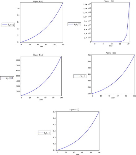We may observe that a small change in $a_0,{\delta }_0,{\delta }_1,r$ and $p_1$ can produce the significant changes in the level of tumour cells. The parameter of model (6(6) $\begin{array}{rl}\frac{\mathrm{d}{u}_1}{\mathrm{d}t}& =a_0{u}_1-2c_0{x}_1^{\ast }{a}_0{u}_1-\frac{{\delta }_0{x}_4^{\ast }}{1+c_1{x}_2^{\ast }}{u}_1+\frac{{\delta }_0{x}_4^{\ast }{x}_1^{\ast }{c}_1}{(1+c_1{x}_2^{\ast }{)}^2}{u}_2-\frac{{\delta }_0{x}_1^{\ast }}{1+c_1{x}_2^{\ast }}{u}_4,\\ \frac{\mathrm{d}{u}_2}{\mathrm{d}t}& =\frac{2a_1{x}_1^{\ast }{c}_2}{(c_2+x_1^{\ast }{}^2{)}^2}{u}_1-d_1{u}_2,\\ \frac{\mathrm{d}{u}_3}{\mathrm{d}t}& =r{u}_4-{\delta }_1{u}_3,\\ \frac{\mathrm{d}{u}_4}{\mathrm{d}t}& =\frac{p_1{x}_5^{\ast }}{g_1+x_5^{\ast }}{u}_4(t-\tau )+\frac{p_1{g}_1{x}_4^{\ast }}{(g_1+x_5^{\ast }{)}^2}{u}_5(t-\tau )-r{u}_4-{\delta }_0{x}_3^{\ast }{u}_4-{\delta }_0{x}_4^{\ast }{u}_3\\ & -{\delta }_1{u}_4-\frac{q_1{x}_4^{\ast }{x}_2^{\ast }}{q_2+x_2^{\ast }}{u}_5--\frac{q_1{x}_5^{\ast }{x}_2^{\ast }}{q_2+x_2^{\ast }}{u}_4-\frac{q_1{x}_4^{\ast }{x}_5^{\ast }}{(q_2+x_2^{\ast }{)}^2}{u}_2,\\ \frac{\mathrm{d}{u}_5}{\mathrm{d}t}& =\frac{p_3{x}_1^{\ast }}{(g_4+x_1^{\ast })(1+\alpha x_2^{\ast })}{u}_4+\frac{p_3{x}_4^{\ast }{g}_4}{(g_4+x_1^{\ast }{)}^2(1+\alpha x_2^{\ast })}{u}_1\\ & -\frac{p_3{x}_1^{\ast }{x}_4^{\ast }\alpha }{(g_4+x_1^{\ast })(1+\alpha x_2^{\ast }{)}^2}{u}_2-{\mu }_2{u}_5.\end{array}$(6) ) is perturbed both positive and negative of their base case values to determine the effect on the output solutions. Figure 1(a–e) shows that the sensitivity of tumour cell population $u_1$, due to small perturbation in $a_0,{\delta }_0,{\delta }_1,r$ and $p_1$. We notice that from Figure 1(b), is insensitive with increasing the value of $a_0$ into the earlier interval, after some time it become highly sensitive. But the other parameters except that $a_0$, are highly very sensitive with increasing their level.

Figure 1. Sensitivity solutions of tumour cell population from (19) to (23) w.r.t a₀, δ₀, δ₁, r and p₁.

5. Applications with numerical simulations

In this section, we have discussed the dynamical behaviour of the systems, we have analysed, graphically. Numerical simulations are carried out using MAPLE and MATLAB packages. We have also tried to show a comparative study between the systems with no therapy, with chemotherapy and with chemo-immunotherapy for tumour-immune evasion system. We present some numerical results of system (4(4) $\begin{array}{rl}\frac{\mathrm{d}{x}_1\left(t\right)}{\mathrm{d}t}& =a_0{x}_1\left(t\right)(1-c_0{x}_1(t\left)\right)-\frac{{\delta }_0{x}_4\left(t\right)x_1\left(t\right)}{1+c_1{x}_2\left(t\right)},\\ \frac{\mathrm{d}{x}_2\left(t\right)}{\mathrm{d}t}& =a_1\frac{x_1^2\left(t\right)}{c_2+x_1^2\left(t\right)}-d_1{x}_2\left(t\right),\\ \frac{\mathrm{d}{x}_3\left(t\right)}{\mathrm{d}t}& =r{x}_4\left(t\right)-{\delta }_1{x}_3\left(t\right),\\ \frac{\mathrm{d}{x}_4\left(t\right)}{\mathrm{d}t}& =\frac{p_1{x}_4(t-\tau )x_5(t-\tau )}{g_1+x_5(t-\tau )}-\frac{q_1{x}_4\left(t\right)x_5\left(t\right)x_2\left(t\right)}{q_2+x_2\left(t\right)}\\ & -r{x}_4\left(t\right)-{\delta }_0{x}_3\left(t\right)x_4\left(t\right)-{\delta }_1{x}_4\left(t\right)+s_1,\\ \frac{\mathrm{d}{x}_5\left(t\right)}{\mathrm{d}t}& =\frac{p_3{x}_4\left(t\right)x_1\left(t\right)}{(g_4+x_1(t\left)\right)(1+\alpha x_2(t\left)\right)}-{\mu }_2{x}_5\left(t\right)+s_2.\end{array}$(4) ), supporting the theoretical analysis. Using the value of Table 1, we consider the following system (24) $\begin{array}{rl}\frac{\mathrm{d}{x}_1\left(t\right)}{\mathrm{d}t}& =0.01946x_1\left(t\right)(1-0.00271x_1(t\left)\right)-\frac{0.000001x_4\left(t\right)x_1\left(t\right)}{1+10x_2\left(t\right)},\\ \frac{\mathrm{d}{x}_2\left(t\right)}{\mathrm{d}t}& =0.03\frac{x_1(t{)}^2}{3+x_1(t{)}^2}-0.0007x_2\left(t\right),\\ \frac{\mathrm{d}{x}_3\left(t\right)}{\mathrm{d}t}& =0.001x_4\left(t\right)-0.000001x_3\left(t\right),\\ \frac{\mathrm{d}{x}_4\left(t\right)}{\mathrm{d}t}& =\frac{0.01245x_4(t-\tau )x_5(t-\tau )}{200+x_5(t-\tau )}-\frac{0.01121x_4\left(t\right)x_5\left(t\right)x_2\left(t\right)}{20+x_2\left(t\right)}-0.001x_4\left(t\right)\\ & -0.000001x_3\left(t\right)x_4\left(t\right)-0.000001x_4\left(t\right)+0.00000246446,\\ \frac{\mathrm{d}{x}_5\left(t\right)}{\mathrm{d}t}& =\frac{0.000025x_4\left(t\right)x_1\left(t\right)}{(0.01+x_1(t\left)\right)(1+0.00000001x_2(t\left)\right)}-10x_5\left(t\right)+\mathrm{0.05.}\end{array}$(24) Clearly the positive tumour-free equilibrium is $I_1=(0,0,0,0.000246207455,0.005{)}^T$. From (7(7) $\mathrm{\Delta }(\lambda ,\tau )={\lambda }^2+A_1\lambda +A_2+(B_1\lambda +B_2){\mathrm{e}}^{-\lambda \tau }=0.$(7) ), we obtain (25) $\begin{array}{rl}& {\lambda }^2-0.01845899975\lambda -0.0001947945975+{\mathrm{e}}^{-13\lambda }(-3.112422190\times {10}^{-7}\lambda \\ & +6.056773505\times {10}^{-9})=0,\end{array}$(25) which has only one positive real roots $\lambda =0.01945999975$ and any other roots have negative real part. Thus, ${\omega }_0=\surd \lambda =0.1394991030437$. For different τ values, we plot the characteristic equation, which is illustrated by numerical simulation in Figure 2(a,b) with initial value $({10}^5,{10}^5,{10}^5,{10}^5,{10}^5{)}^{\mathrm{T}}$.

Figure 2. Plots the characteristic equation of (25(25) $\begin{array}{rl}& {\lambda }^2-0.01845899975\lambda -0.0001947945975+{\mathrm{e}}^{-13\lambda }(-3.112422190\times {10}^{-7}\lambda \\ & +6.056773505\times {10}^{-9})=0,\end{array}$(25) ) for different τ values (Table 1).

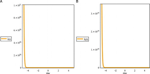
Figure 2(a,b) shows that the characteristic equation of (25(25) $\begin{array}{rl}& {\lambda }^2-0.01845899975\lambda -0.0001947945975+{\mathrm{e}}^{-13\lambda }(-3.112422190\times {10}^{-7}\lambda \\ & +6.056773505\times {10}^{-9})=0,\end{array}$(25) ) has negative real parts. Then the system (24(24) $\begin{array}{rl}\frac{\mathrm{d}{x}_1\left(t\right)}{\mathrm{d}t}& =0.01946x_1\left(t\right)(1-0.00271x_1(t\left)\right)-\frac{0.000001x_4\left(t\right)x_1\left(t\right)}{1+10x_2\left(t\right)},\\ \frac{\mathrm{d}{x}_2\left(t\right)}{\mathrm{d}t}& =0.03\frac{x_1(t{)}^2}{3+x_1(t{)}^2}-0.0007x_2\left(t\right),\\ \frac{\mathrm{d}{x}_3\left(t\right)}{\mathrm{d}t}& =0.001x_4\left(t\right)-0.000001x_3\left(t\right),\\ \frac{\mathrm{d}{x}_4\left(t\right)}{\mathrm{d}t}& =\frac{0.01245x_4(t-\tau )x_5(t-\tau )}{200+x_5(t-\tau )}-\frac{0.01121x_4\left(t\right)x_5\left(t\right)x_2\left(t\right)}{20+x_2\left(t\right)}-0.001x_4\left(t\right)\\ & -0.000001x_3\left(t\right)x_4\left(t\right)-0.000001x_4\left(t\right)+0.00000246446,\\ \frac{\mathrm{d}{x}_5\left(t\right)}{\mathrm{d}t}& =\frac{0.000025x_4\left(t\right)x_1\left(t\right)}{(0.01+x_1(t\left)\right)(1+0.00000001x_2(t\left)\right)}-10x_5\left(t\right)+\mathrm{0.05.}\end{array}$(24) ) is always stable in tumour-free equilibrium.

The optimal system has been solved numerically and the results have been presented graphically. There are two systems of DDEs, the first system (11(11) $\begin{array}{rl}\frac{\mathrm{d}T\left(t\right)}{\mathrm{d}t}& =a_{0}T\left(t\right)(1-c_{0}T(t\left)\right)-\frac{{\delta }_{0}E\left(t\right)T\left(t\right)}{1+c_{1}B\left(t\right)},\\ \frac{\mathrm{d}B\left(t\right)}{\mathrm{d}t}& =a_1\frac{T^2\left(t\right)}{c_2+T^2\left(t\right)}-d_{1}B\left(t\right),\\ \frac{\mathrm{d}R\left(t\right)}{\mathrm{d}t}& =rE\left(t\right)-{\delta }_{1}R\left(t\right),\\ \frac{\mathrm{d}E\left(t\right)}{\mathrm{d}t}& =\frac{p_{1}E(t-\tau )I(t-\tau )}{g_1+I(t-\tau )}-\frac{q_{1}E\left(t\right)I\left(t\right)B\left(t\right)}{q_2+B\left(t\right)}-rE\left(t\right)-{\delta }_{0}R\left(t\right)E\left(t\right)-{\delta }_{1}E\left(t\right)+\rho \left(t\right)s_1,\\ \frac{\mathrm{d}I\left(t\right)}{\mathrm{d}t}& =\frac{p_{3}E\left(t\right)T\left(t\right)}{(g_4+T(t\left)\right)(1+\alpha B(t\left)\right)}-{\mu }_{2}I\left(t\right)+s_2.\\ \frac{\mathrm{d}M\left(t\right)}{\mathrm{d}t}& =\eta \left(t\right)-\beta M\left(t\right),\end{array}$(11) ) being the state equations involving the control and the second (16(16) $\begin{array}{rl}{\lambda }_1^{\mathrm{\prime }}\left(t\right)& =1-{\lambda }_1\left(a_0-2a_0{c}_{0}T-{\delta }_{0}E\right)-{\lambda }_2\left(\frac{2a_{1}T{c}_2}{(c_2+T^2{)}^2}\right)-{\lambda }_5\frac{p_{3}E{g}_4}{(g_4+T{)}^2(1+\alpha B)}\\ {\lambda }_2^{\mathrm{\prime }}\left(t\right)& =-1-{\lambda }_1\left(\frac{{\delta }_0{c}_{1}ET}{(1+c_{1}B{)}^2}\right)+{\lambda }_{2}d+{\lambda }_5\left(\frac{p_3\alpha ET}{(g_4+T)(1+\alpha B{)}^2}\right)\\ {\lambda }_3^{\mathrm{\prime }}\left(t\right)& ==-1-{\lambda }_3(-{\delta }_1)-{\lambda }_4(-{\delta }_{0}E)\\ {\lambda }_4^{\mathrm{\prime }}\left(t\right)& =-1-{\lambda }_1\left(\frac{-{\delta }_{0}T}{1+c_{1}B\left(t\right)}\right)-{\lambda }_3\left(r\right)-{\lambda }_4(-r-{\delta }_{0}R-{\delta }_1)\\ & -{\lambda }_4(t+\tau )-{\chi }_{[0,t_f-\tau ]}\frac{p_{1}I}{g_1+I}-{\lambda }_5\frac{p_{3}T}{(g_4+T)(1+\alpha B)}\\ {\lambda }_5^{\mathrm{\prime }}\left(t\right)& =-1-{\lambda }_4(t+\tau ){\chi }_{[0,t_f-\tau ]}\frac{p_1{g}_{1}E}{(g_1+I{)}^2}-{\lambda }_5(-{\mu }_2)\\ {\lambda }_6^{\mathrm{\prime }}\left(t\right)& =-1-{\lambda }_6(-\beta ).\end{array}$(16) ) being the adjoint equations ${\lambda }_i$'s (i=1,2,…,5). An initial guess was made for ${\lambda }_i$'s ($i=1,2,\dots ,5$) gives an initial guess for the control. From here the state equations were solved using the initial condition. Our findings leading to the approximation of the optimal controls (11(11) $\begin{array}{rl}\frac{\mathrm{d}T\left(t\right)}{\mathrm{d}t}& =a_{0}T\left(t\right)(1-c_{0}T(t\left)\right)-\frac{{\delta }_{0}E\left(t\right)T\left(t\right)}{1+c_{1}B\left(t\right)},\\ \frac{\mathrm{d}B\left(t\right)}{\mathrm{d}t}& =a_1\frac{T^2\left(t\right)}{c_2+T^2\left(t\right)}-d_{1}B\left(t\right),\\ \frac{\mathrm{d}R\left(t\right)}{\mathrm{d}t}& =rE\left(t\right)-{\delta }_{1}R\left(t\right),\\ \frac{\mathrm{d}E\left(t\right)}{\mathrm{d}t}& =\frac{p_{1}E(t-\tau )I(t-\tau )}{g_1+I(t-\tau )}-\frac{q_{1}E\left(t\right)I\left(t\right)B\left(t\right)}{q_2+B\left(t\right)}-rE\left(t\right)-{\delta }_{0}R\left(t\right)E\left(t\right)-{\delta }_{1}E\left(t\right)+\rho \left(t\right)s_1,\\ \frac{\mathrm{d}I\left(t\right)}{\mathrm{d}t}& =\frac{p_{3}E\left(t\right)T\left(t\right)}{(g_4+T(t\left)\right)(1+\alpha B(t\left)\right)}-{\mu }_{2}I\left(t\right)+s_2.\\ \frac{\mathrm{d}M\left(t\right)}{\mathrm{d}t}& =\eta \left(t\right)-\beta M\left(t\right),\end{array}$(11) ) are carried out using the forward Euler method for the state system and backward difference approximation for the adjoint system. We assume that the step size h, such that $\tau =mh$ and $t_f-t_0=nh$, where $(m,b)\in {\mathbb{N}}^2$. We define the state, adjoint and control variables at the mesh points. An initial guess is given for the controls ρ and η, which are then updated continuously until the objective functional satisfies the conditions. However, there are several major problems to overcome when solving DDEs. We choose a set of parameter values are taken from Table 2. We solve the optimality system to determine the optimal control situation (i.e., drug strategy), and predict the evolution of the system had taken each control strategy in 10 days.

Table 2. Parameters description and values.

Parameter	Mouse data	Human data	Source
$p_1$	0.1245	0.1245	[15]
$g_1$	2 $\times {10}^7$	2 $\times {10}^7$	[15]
${\mu }_2$	10	10	Estimated
$a_0$	2 $\times {10}^{-3}$	4.31$\times {10}^{-1}$	Estimated
$c_0$	1.02 $\times {10}^{-9}$	2.17 $\times {10}^{-8}$	[9]
${\delta }_0$	3.23 $\times {10}^{-7}$	7.13 $\times {10}^{-10}$	[9,10]
${\mu }_3$	10	10	[15]
$p_3$	6 $\times {10}^{-1}$	6 $\times {10}^{-1}$	Estimated
$g_4$	1 $\times {10}^5$	1 $\times {10}^5$	[9]
β	9 $\times {10}^{-1}$	9 $\times {10}^{-1}$	[5]
$a_0$	0.1946	0.1946	[28]
r	0.01	0.01	[14]

Figure 3(a–c) shows results of our simulations in the three treatment regimes along with the corresponding experimental data for Mouse data (Using Table 2). Figure 3(a) shows that tumour size level of no treatment therapy. In this case the tumour growth becomes immediately uncontrolled. Using chemotherapy with tumour-immune system, the tumour growth became to control for 6 days, after that the tumour growth immediately uncontrolled which can be shown from Figure 3(b). Finally, we show the both chemo-immuno therapy treatment of our model, the system becomes control within 8 days only. After, the tumour-immune system grows up quickly becomes uncontrolled.

Figure 3. The dynamics of the tumour size in three treatment regimes. Shown are the results of the numerical simulations for Mouse data corresponding from Table 2 with initial condition $T\left(t\right)={10}^5$, $B\left(t\right)={10}^5$, $R\left(t\right)={10}^5$, $E\left(t\right)={10}^5$, $I\left(t\right)={10}^5$, $M\left(t\right)={10}^5$.

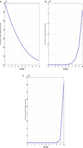
Figure 4(a–c) shows results of our simulations in the three treatment regimes along with the corresponding experimental data for human data (Using Table 2). Figure 4(a) shows that tumour size level of no treatment therapy. In this case the tumour growth becomes immediately uncontrolled. Even though, using chemotherapy with tumour-immune system, the tumour growth became to uncontrolled, which it can be shown from Figure 4(b). Finally, we show the both chemo-immuno therapy treatment for our model, the system becomes control within 7 days only. After, the tumour-immune system grows up quickly becomes uncontrolled.

Figure 4. The dynamics of the tumour size in three treatment regimes. Shown are the results of the numerical simulations for human data corresponding from Table 2 with initial condition $T\left(t\right)={10}^5$, $B\left(t\right)={10}^5$, $R\left(t\right)={10}^5$, $E\left(t\right)={10}^5$, $I\left(t\right)={10}^5$, $M\left(t\right)={10}^5$.

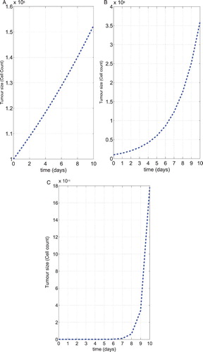
Figure 5. The optimal control graph for the chemo therapeutic drug control (M) using the parameter values given in Table 2 with $B_{\rho }=1$ and $B_{\eta }=2$ for mouse and human data.

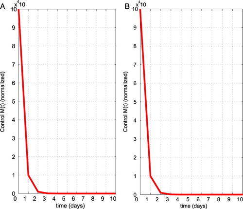
To compare the tumour growth in all treatment regimes. It is clear that while monotherapy results in a slowing down of the tumour growth, the tumour is still able to escape immuno surveillance and grow uncontrolled. Only in the case of dual therapy is the immune system able to eradicate the tumour within 8 days.

6. Conclusion

We have examined a model incorporating interacting tumour and immune cell populations and their responses to chemo-immunotherapy treatment. The dynamics of the system without treatment reveal two equilibrium points for a specific parameter case: trivial equilibrium and tumour-free equilibrium. We presented the non-negativity and boundedness of solutions, existence of steady states of our model. The immune system inhibitory effects (such as blocking IL-2 production and inhibiting antigen-specific T-cell activation) and tumour-stimulating effects (such as increasing blood supply to tumour cells in order to enhance the tumour's ability to metastasize) of TGF-$\beta$ provide explanation for enhanced tumour growth and failure of the host immune system. In order to counteract this occurrence, the model was extended to include a novel therapeutic strategy using the chemo-immunotherapy treatment without TGF-$\beta$ cells. For using the both therapies level, from the very beginning the tumour controlled within 8 days. After some time, the tumour can be grow up uncontrolled.

Acknowledgements

The authors are grateful to the anonymous reviewers for constructive suggestions and valuable comments, which improved the quality of the paper.

Disclosure statement

No potential conflict of interest was reported by the authors.

Appendix 1

Proof

Proof of Proposition 2.1.2.

The first equation of system (4(4) $\begin{array}{rl}\frac{\mathrm{d}{x}_1\left(t\right)}{\mathrm{d}t}& =a_0{x}_1\left(t\right)(1-c_0{x}_1(t\left)\right)-\frac{{\delta }_0{x}_4\left(t\right)x_1\left(t\right)}{1+c_1{x}_2\left(t\right)},\\ \frac{\mathrm{d}{x}_2\left(t\right)}{\mathrm{d}t}& =a_1\frac{x_1^2\left(t\right)}{c_2+x_1^2\left(t\right)}-d_1{x}_2\left(t\right),\\ \frac{\mathrm{d}{x}_3\left(t\right)}{\mathrm{d}t}& =r{x}_4\left(t\right)-{\delta }_1{x}_3\left(t\right),\\ \frac{\mathrm{d}{x}_4\left(t\right)}{\mathrm{d}t}& =\frac{p_1{x}_4(t-\tau )x_5(t-\tau )}{g_1+x_5(t-\tau )}-\frac{q_1{x}_4\left(t\right)x_5\left(t\right)x_2\left(t\right)}{q_2+x_2\left(t\right)}\\ & -r{x}_4\left(t\right)-{\delta }_0{x}_3\left(t\right)x_4\left(t\right)-{\delta }_1{x}_4\left(t\right)+s_1,\\ \frac{\mathrm{d}{x}_5\left(t\right)}{\mathrm{d}t}& =\frac{p_3{x}_4\left(t\right)x_1\left(t\right)}{(g_4+x_1(t\left)\right)(1+\alpha x_2(t\left)\right)}-{\mu }_2{x}_5\left(t\right)+s_2.\end{array}$(4) ), we have (A1) $\frac{\mathrm{d}{x}_1\left(t\right)}{\mathrm{d}t}\le a_0{x}_1\left(t\right)(1-c_0{x}_1(t\left)\right)-\frac{{\delta }_0{x}_4\left(t\right)x_1\left(t\right)}{1+c_1{x}_2\left(t\right)}\le a_0{x}_1\left(t\right)(1-c_0{x}_1(t\left)\right)=M_2.$(A1) From equations (A1(A1) $\frac{\mathrm{d}{x}_1\left(t\right)}{\mathrm{d}t}\le a_0{x}_1\left(t\right)(1-c_0{x}_1(t\left)\right)-\frac{{\delta }_0{x}_4\left(t\right)x_1\left(t\right)}{1+c_1{x}_2\left(t\right)}\le a_0{x}_1\left(t\right)(1-c_0{x}_1(t\left)\right)=M_2.$(A1) ), we observe that (A2) $M_1=max(1/c_0,x_1(0\left)\right).$(A2) From the second equation of system (4(4) $\begin{array}{rl}\frac{\mathrm{d}{x}_1\left(t\right)}{\mathrm{d}t}& =a_0{x}_1\left(t\right)(1-c_0{x}_1(t\left)\right)-\frac{{\delta }_0{x}_4\left(t\right)x_1\left(t\right)}{1+c_1{x}_2\left(t\right)},\\ \frac{\mathrm{d}{x}_2\left(t\right)}{\mathrm{d}t}& =a_1\frac{x_1^2\left(t\right)}{c_2+x_1^2\left(t\right)}-d_1{x}_2\left(t\right),\\ \frac{\mathrm{d}{x}_3\left(t\right)}{\mathrm{d}t}& =r{x}_4\left(t\right)-{\delta }_1{x}_3\left(t\right),\\ \frac{\mathrm{d}{x}_4\left(t\right)}{\mathrm{d}t}& =\frac{p_1{x}_4(t-\tau )x_5(t-\tau )}{g_1+x_5(t-\tau )}-\frac{q_1{x}_4\left(t\right)x_5\left(t\right)x_2\left(t\right)}{q_2+x_2\left(t\right)}\\ & -r{x}_4\left(t\right)-{\delta }_0{x}_3\left(t\right)x_4\left(t\right)-{\delta }_1{x}_4\left(t\right)+s_1,\\ \frac{\mathrm{d}{x}_5\left(t\right)}{\mathrm{d}t}& =\frac{p_3{x}_4\left(t\right)x_1\left(t\right)}{(g_4+x_1(t\left)\right)(1+\alpha x_2(t\left)\right)}-{\mu }_2{x}_5\left(t\right)+s_2.\end{array}$(4) ), we obtain (A3) $x_2\left(t\right)\le {\mathrm{e}}^{(-\mathrm{d}t)}\left(x_2\left(0\right)+{\int }_0^t{a}_1\frac{x_1(s{)}^2}{c_2+x_1(s{)}^2}{\mathrm{e}}^{\left(\mathrm{d}s\right)}\mathrm{d}s\right)=M_2,$(A3) Note that from third equation of system (4(4) $\begin{array}{rl}\frac{\mathrm{d}{x}_1\left(t\right)}{\mathrm{d}t}& =a_0{x}_1\left(t\right)(1-c_0{x}_1(t\left)\right)-\frac{{\delta }_0{x}_4\left(t\right)x_1\left(t\right)}{1+c_1{x}_2\left(t\right)},\\ \frac{\mathrm{d}{x}_2\left(t\right)}{\mathrm{d}t}& =a_1\frac{x_1^2\left(t\right)}{c_2+x_1^2\left(t\right)}-d_1{x}_2\left(t\right),\\ \frac{\mathrm{d}{x}_3\left(t\right)}{\mathrm{d}t}& =r{x}_4\left(t\right)-{\delta }_1{x}_3\left(t\right),\\ \frac{\mathrm{d}{x}_4\left(t\right)}{\mathrm{d}t}& =\frac{p_1{x}_4(t-\tau )x_5(t-\tau )}{g_1+x_5(t-\tau )}-\frac{q_1{x}_4\left(t\right)x_5\left(t\right)x_2\left(t\right)}{q_2+x_2\left(t\right)}\\ & -r{x}_4\left(t\right)-{\delta }_0{x}_3\left(t\right)x_4\left(t\right)-{\delta }_1{x}_4\left(t\right)+s_1,\\ \frac{\mathrm{d}{x}_5\left(t\right)}{\mathrm{d}t}& =\frac{p_3{x}_4\left(t\right)x_1\left(t\right)}{(g_4+x_1(t\left)\right)(1+\alpha x_2(t\left)\right)}-{\mu }_2{x}_5\left(t\right)+s_2.\end{array}$(4) ), we get (A4) $x_3\left(t\right)\le {\mathrm{e}}^{(-{\delta }_{1}t)}\left(x_3\left(0\right)+{\int }_0^{t}r{x}_4\left(s\right){\mathrm{e}}^{\left({\delta }_{1}s\right)}\mathrm{d}s\right)=M_3.$(A4) Further, we simplify fourth equations from the system (4(4) $\begin{array}{rl}\frac{\mathrm{d}{x}_1\left(t\right)}{\mathrm{d}t}& =a_0{x}_1\left(t\right)(1-c_0{x}_1(t\left)\right)-\frac{{\delta }_0{x}_4\left(t\right)x_1\left(t\right)}{1+c_1{x}_2\left(t\right)},\\ \frac{\mathrm{d}{x}_2\left(t\right)}{\mathrm{d}t}& =a_1\frac{x_1^2\left(t\right)}{c_2+x_1^2\left(t\right)}-d_1{x}_2\left(t\right),\\ \frac{\mathrm{d}{x}_3\left(t\right)}{\mathrm{d}t}& =r{x}_4\left(t\right)-{\delta }_1{x}_3\left(t\right),\\ \frac{\mathrm{d}{x}_4\left(t\right)}{\mathrm{d}t}& =\frac{p_1{x}_4(t-\tau )x_5(t-\tau )}{g_1+x_5(t-\tau )}-\frac{q_1{x}_4\left(t\right)x_5\left(t\right)x_2\left(t\right)}{q_2+x_2\left(t\right)}\\ & -r{x}_4\left(t\right)-{\delta }_0{x}_3\left(t\right)x_4\left(t\right)-{\delta }_1{x}_4\left(t\right)+s_1,\\ \frac{\mathrm{d}{x}_5\left(t\right)}{\mathrm{d}t}& =\frac{p_3{x}_4\left(t\right)x_1\left(t\right)}{(g_4+x_1(t\left)\right)(1+\alpha x_2(t\left)\right)}-{\mu }_2{x}_5\left(t\right)+s_2.\end{array}$(4) ), we obtain (A5) $\begin{array}{rl}{x}_4\left(t\right)& \le {\mathrm{e}}^{-{\int }_0^t\left(q{x}_5\right(\xi )+r+{\delta }_0{x}_3(\xi )+{\delta }_1)\mathrm{d}\xi }\left(\left(x_4\left(0\right)+{\int }_0^t{s}_1+\frac{p_1{x}_4(t-\tau )x_5(t-\tau )}{g_1+x_5(t-\tau )}\right)\right.\\ & \times \left.{\mathrm{e}}^{{\int }_s^t\left(q{x}_5\right(\xi )+r+{\delta }_0{x}_3(\xi \left)\phantom{\frac{p_1{x}_4(t-\tau )x_5(t-\tau )}{g_1+x_5(t-\tau )}}\right)\mathrm{d}\xi }\mathrm{d}s\right).\end{array}$(A5) Since $x_5/(g_1+x_5)<1$, and by using Lemma 2.1, the above equation (A5(A5) $\begin{array}{rl}{x}_4\left(t\right)& \le {\mathrm{e}}^{-{\int }_0^t\left(q{x}_5\right(\xi )+r+{\delta }_0{x}_3(\xi )+{\delta }_1)\mathrm{d}\xi }\left(\left(x_4\left(0\right)+{\int }_0^t{s}_1+\frac{p_1{x}_4(t-\tau )x_5(t-\tau )}{g_1+x_5(t-\tau )}\right)\right.\\ & \times \left.{\mathrm{e}}^{{\int }_s^t\left(q{x}_5\right(\xi )+r+{\delta }_0{x}_3(\xi \left)\phantom{\frac{p_1{x}_4(t-\tau )x_5(t-\tau )}{g_1+x_5(t-\tau )}}\right)\mathrm{d}\xi }\mathrm{d}s\right).\end{array}$(A5) ) becomes, (A6) $\begin{array}{rl}{x}_4\left(t\right)& \le {\mathrm{e}}^{-{\int }_0^t\left(q{x}_5\right(\xi )+r+{\delta }_0{x}_3(\xi )+{\delta }_1)\mathrm{d}\xi }\left(\left(x_4\left(0\right)+{\int }_0^t{s}_1+p_1{x}_4(t-\tau )\right)\right.\\ & \left.{\mathrm{e}}^{{\int }_s^t\left(q{x}_5\right(\xi )+r+{\delta }_0{x}_3(\xi \left)\right)\mathrm{d}\xi }\mathrm{d}s\right),\end{array}$(A6) Hence $x_4\left(t\right)\le M_4$, where $M_4$ is uniformly bounded on $[0,\tau ]$.

The fifth equation from the system (4(4) $\begin{array}{rl}\frac{\mathrm{d}{x}_1\left(t\right)}{\mathrm{d}t}& =a_0{x}_1\left(t\right)(1-c_0{x}_1(t\left)\right)-\frac{{\delta }_0{x}_4\left(t\right)x_1\left(t\right)}{1+c_1{x}_2\left(t\right)},\\ \frac{\mathrm{d}{x}_2\left(t\right)}{\mathrm{d}t}& =a_1\frac{x_1^2\left(t\right)}{c_2+x_1^2\left(t\right)}-d_1{x}_2\left(t\right),\\ \frac{\mathrm{d}{x}_3\left(t\right)}{\mathrm{d}t}& =r{x}_4\left(t\right)-{\delta }_1{x}_3\left(t\right),\\ \frac{\mathrm{d}{x}_4\left(t\right)}{\mathrm{d}t}& =\frac{p_1{x}_4(t-\tau )x_5(t-\tau )}{g_1+x_5(t-\tau )}-\frac{q_1{x}_4\left(t\right)x_5\left(t\right)x_2\left(t\right)}{q_2+x_2\left(t\right)}\\ & -r{x}_4\left(t\right)-{\delta }_0{x}_3\left(t\right)x_4\left(t\right)-{\delta }_1{x}_4\left(t\right)+s_1,\\ \frac{\mathrm{d}{x}_5\left(t\right)}{\mathrm{d}t}& =\frac{p_3{x}_4\left(t\right)x_1\left(t\right)}{(g_4+x_1(t\left)\right)(1+\alpha x_2(t\left)\right)}-{\mu }_2{x}_5\left(t\right)+s_2.\end{array}$(4) ), it gives (A7) $\frac{\mathrm{d}{x}_5\left(t\right)}{\mathrm{d}t}={\mathrm{e}}^{-\left({\mu }_{2}t\right)}\left(x_5\left(0\right)+{\int }_0^t\left(s_2+\frac{p_3{x}_4\left(s\right)x_1\left(s\right)}{(g_4+x_1(s\left)\right)(1+\alpha x_2(s\left)\right)}\right){\mathrm{e}}^{\left({\mu }_{2}s\right)}\mathrm{d}s\right).$(A7) Since $x_1/(g_4+x_1)<1$, and ${\mathrm{e}}^{(-{\mu }_{2}t)}\in (0,1]$, and by using Lemma 2.1, the above equation (A7(A7) $\frac{\mathrm{d}{x}_5\left(t\right)}{\mathrm{d}t}={\mathrm{e}}^{-\left({\mu }_{2}t\right)}\left(x_5\left(0\right)+{\int }_0^t\left(s_2+\frac{p_3{x}_4\left(s\right)x_1\left(s\right)}{(g_4+x_1(s\left)\right)(1+\alpha x_2(s\left)\right)}\right){\mathrm{e}}^{\left({\mu }_{2}s\right)}\mathrm{d}s\right).$(A7) ) becomes, (A8) $\frac{\mathrm{d}{x}_5\left(t\right)}{\mathrm{d}t}=x_5\left(0\right)+\frac{s_2}{{\mu }_2}{\mathrm{e}}^{\left({\mu }_{2}t\right)}+{\int }_0^t\frac{p_3{x}_4\left(s\right)}{1+\alpha x_2\left(s\right)}{\mathrm{e}}^{\left({\mu }_{2}s\right)}\mathrm{d}s.$(A8)

The generalized Gronwall Lemma gives $x_4\left(t\right)\le M_4$ where $M_4$ is uniformly bounded. It follows that if $(x_1,x_2,x_3,x_4,x_5)$ is a solution of (4(4) $\begin{array}{rl}\frac{\mathrm{d}{x}_1\left(t\right)}{\mathrm{d}t}& =a_0{x}_1\left(t\right)(1-c_0{x}_1(t\left)\right)-\frac{{\delta }_0{x}_4\left(t\right)x_1\left(t\right)}{1+c_1{x}_2\left(t\right)},\\ \frac{\mathrm{d}{x}_2\left(t\right)}{\mathrm{d}t}& =a_1\frac{x_1^2\left(t\right)}{c_2+x_1^2\left(t\right)}-d_1{x}_2\left(t\right),\\ \frac{\mathrm{d}{x}_3\left(t\right)}{\mathrm{d}t}& =r{x}_4\left(t\right)-{\delta }_1{x}_3\left(t\right),\\ \frac{\mathrm{d}{x}_4\left(t\right)}{\mathrm{d}t}& =\frac{p_1{x}_4(t-\tau )x_5(t-\tau )}{g_1+x_5(t-\tau )}-\frac{q_1{x}_4\left(t\right)x_5\left(t\right)x_2\left(t\right)}{q_2+x_2\left(t\right)}\\ & -r{x}_4\left(t\right)-{\delta }_0{x}_3\left(t\right)x_4\left(t\right)-{\delta }_1{x}_4\left(t\right)+s_1,\\ \frac{\mathrm{d}{x}_5\left(t\right)}{\mathrm{d}t}& =\frac{p_3{x}_4\left(t\right)x_1\left(t\right)}{(g_4+x_1(t\left)\right)(1+\alpha x_2(t\left)\right)}-{\mu }_2{x}_5\left(t\right)+s_2.\end{array}$(4) ), then $(x_1,x_2,x_3,x_4,x_5)<(M_1,M_2,M_3,M_4,M_5)$ for all t. This shows that the solutions of model (4(4) $\begin{array}{rl}\frac{\mathrm{d}{x}_1\left(t\right)}{\mathrm{d}t}& =a_0{x}_1\left(t\right)(1-c_0{x}_1(t\left)\right)-\frac{{\delta }_0{x}_4\left(t\right)x_1\left(t\right)}{1+c_1{x}_2\left(t\right)},\\ \frac{\mathrm{d}{x}_2\left(t\right)}{\mathrm{d}t}& =a_1\frac{x_1^2\left(t\right)}{c_2+x_1^2\left(t\right)}-d_1{x}_2\left(t\right),\\ \frac{\mathrm{d}{x}_3\left(t\right)}{\mathrm{d}t}& =r{x}_4\left(t\right)-{\delta }_1{x}_3\left(t\right),\\ \frac{\mathrm{d}{x}_4\left(t\right)}{\mathrm{d}t}& =\frac{p_1{x}_4(t-\tau )x_5(t-\tau )}{g_1+x_5(t-\tau )}-\frac{q_1{x}_4\left(t\right)x_5\left(t\right)x_2\left(t\right)}{q_2+x_2\left(t\right)}\\ & -r{x}_4\left(t\right)-{\delta }_0{x}_3\left(t\right)x_4\left(t\right)-{\delta }_1{x}_4\left(t\right)+s_1,\\ \frac{\mathrm{d}{x}_5\left(t\right)}{\mathrm{d}t}& =\frac{p_3{x}_4\left(t\right)x_1\left(t\right)}{(g_4+x_1(t\left)\right)(1+\alpha x_2(t\left)\right)}-{\mu }_2{x}_5\left(t\right)+s_2.\end{array}$(4) ) are uniformly bounded. This completes the proof.

Appendix 2

For $\tau =0$, the above equation (7(7) $\mathrm{\Delta }(\lambda ,\tau )={\lambda }^2+A_1\lambda +A_2+(B_1\lambda +B_2){\mathrm{e}}^{-\lambda \tau }=0.$(7) ) becomes as follows: ${\lambda }^2+(A_1+B_1)\lambda +(A_2+B_2)=0.$ By Routh–Hurwitz criteria, the corresponding system without delay is locally asymptotically stable around the infection equilibrium if following conditions are satisfied:

• $(A_1+B_1)>0$ and $(A_2+B_2)>0$.

Now, we put $\lambda \left(\tau \right)=\mu \left(\tau \right)+i\nu \left(\tau \right)$ in Equation (7(7) $\mathrm{\Delta }(\lambda ,\tau )={\lambda }^2+A_1\lambda +A_2+(B_1\lambda +B_2){\mathrm{e}}^{-\lambda \tau }=0.$(7) ), we obtain (A9) $\begin{array}{rl}& {\mu }^2-{\nu }^2+A_1\mu +A_2+B_1\mu \cos \mu \tau +B_1\mu \sin \nu \tau -B_1\nu \cos \nu \tau \\ & +B_1\nu \sin \mu \tau +B_2\cos \mu \tau +B_2\sin \nu \tau =0;\\ & 2\mu \nu +A_1\nu +B_1\mu \cos \nu \tau -B_1\mu \sin \mu \tau +B_1\nu \cos \mu \tau +B_1\nu \sin \mu \tau \\ & +B_2\cos \nu \tau -B_2\sin \nu \tau =0.\end{array}$(A9)

A.1. Criterion for preservation of stability or instability and bifurcation results

We have to determine the change of stability of $I_2$ for some τ for which $\mu \left(\tau \right)=0,\nu \left(\tau \right)\ne 0$, that is, when λ will be purely imaginary. Let ${\tau }^{\ast }$ be such that $\mu \left({\tau }^{\ast }\right)=0$ and $\nu \left({\tau }^{\ast }\right)={\nu }_0\ne 0$. In this case the steady state loses stability and eventually become unstable when $\mu \left({\tau }^{\ast }\right)$ becomes positive. However, if such a $\nu \left({\tau }^{\ast }\right)$ does not exists, that is, if λ be not purely imaginary for $\tau ={\tau }^{\ast }$, then $I_2$ is always stable. We will show that it is the case with Equation (7(7) $\mathrm{\Delta }(\lambda ,\tau )={\lambda }^2+A_1\lambda +A_2+(B_1\lambda +B_2){\mathrm{e}}^{-\lambda \tau }=0.$(7) ). Now when λ is purely imaginary in (A9(A9) $\begin{array}{rl}& {\mu }^2-{\nu }^2+A_1\mu +A_2+B_1\mu \cos \mu \tau +B_1\mu \sin \nu \tau -B_1\nu \cos \nu \tau \\ & +B_1\nu \sin \mu \tau +B_2\cos \mu \tau +B_2\sin \nu \tau =0;\\ & 2\mu \nu +A_1\nu +B_1\mu \cos \nu \tau -B_1\mu \sin \mu \tau +B_1\nu \cos \mu \tau +B_1\nu \sin \mu \tau \\ & +B_2\cos \nu \tau -B_2\sin \nu \tau =0.\end{array}$(A9) ) reduce to (A10) $\begin{array}{rl}{\nu }^2-A_2& =B_1\nu \sin \nu \tau +B_2\cos \nu \tau ,\\ A_1\nu & =B_2\sin \nu \tau -B_1\nu \cos \nu \tau .\end{array}$(A10) Now squaring and adding above Equation (A10(A10) $\begin{array}{rl}{\nu }^2-A_2& =B_1\nu \sin \nu \tau +B_2\cos \nu \tau ,\\ A_1\nu & =B_2\sin \nu \tau -B_1\nu \cos \nu \tau .\end{array}$(A10) ) we get, (A11) ${\nu }^4+{\nu }^2(A_1^2-2A_2-B_1^2)+A_2^2-B_2^2=0,$(A11) putting $y={\nu }^2$ into the above Equation (A11(A11) ${\nu }^4+{\nu }^2(A_1^2-2A_2-B_1^2)+A_2^2-B_2^2=0,$(A11) ), we can obtain the following quadratic equation: (A12) $\mathrm{\Psi }\left(y\right)=y^2+H_{1}u+H_2=0,$(A12) where $\begin{array}{rl}{H}_1& =A_1^2-2A_2-B_1^2>0\\ H_2& =A_2^2-B_2^2>0.\end{array}$ If we assume that $H_1>0$ and $H_2>0$, then the above Equation (A12(A12) $\mathrm{\Psi }\left(y\right)=y^2+H_{1}u+H_2=0,$(A12) ) has no positive root. In fact, it is observed that, (A13) $\begin{array}{r}\frac{\mathrm{d}\mathrm{\Psi }\left(y\right)}{\mathrm{d}t}=2y+H_1=0,\end{array}$(A13) has no positive real root by Descarte's rule of sign. Thus if, $H_1>0$ and $H_2>0$ then there is no ν such that $i\nu$ is an eigenvalue of the characteristic equation (7(7) $\mathrm{\Delta }(\lambda ,\tau )={\lambda }^2+A_1\lambda +A_2+(B_1\lambda +B_2){\mathrm{e}}^{-\lambda \tau }=0.$(7) ), that is, λ will never be a purely imaginary root of Equation (7(7) $\mathrm{\Delta }(\lambda ,\tau )={\lambda }^2+A_1\lambda +A_2+(B_1\lambda +B_2){\mathrm{e}}^{-\lambda \tau }=0.$(7) ). Thus all the real parts of all eigenvalues of (7(7) $\mathrm{\Delta }(\lambda ,\tau )={\lambda }^2+A_1\lambda +A_2+(B_1\lambda +B_2){\mathrm{e}}^{-\lambda \tau }=0.$(7) ) are negative for all $\tau \ge 0$. □

Proof

Proof of Theorem 2.3.

Now if any one of $H_1$ and $H_2$ is negative then $\mathrm{\Psi }\left(y\right)=0$ and hence Equation (A12(A12) $\mathrm{\Psi }\left(y\right)=y^2+H_{1}u+H_2=0,$(A12) ) has positive root ${\nu }_0$. This implies that the characteristic equation (7(7) $\mathrm{\Delta }(\lambda ,\tau )={\lambda }^2+A_1\lambda +A_2+(B_1\lambda +B_2){\mathrm{e}}^{-\lambda \tau }=0.$(7) ) has a pair of purely imaginary roots $\pm i{\nu }_0$.

From (A10(A10) $\begin{array}{rl}{\nu }^2-A_2& =B_1\nu \sin \nu \tau +B_2\cos \nu \tau ,\\ A_1\nu & =B_2\sin \nu \tau -B_1\nu \cos \nu \tau .\end{array}$(A10) ), we have (A14) ${\tau }_j^{\ast }=\frac{1}{{\nu }_0}\arccos \left(\frac{{\nu }_0^2(B_2-A_1{B}_1)-A_2{B}_2}{B_1^2{\nu }_0^2+B_2^2}\right)+\frac{2j\mathrm{\Pi }}{{\omega }_0},j=0,1,2,3,\dots ,$(A14) Now, we determine sign $\left(\mathrm{d}Re\left(\lambda \right)/\mathrm{d}\tau \right){|}_{\tau ={\tau }^{\ast }}$ where sign is the signum function and $Re\left(\lambda \right)$ is a real part of λ. By using the following mathematical calculation we can say that the tumour-free steady state of model (6(6) $\begin{array}{rl}\frac{\mathrm{d}{u}_1}{\mathrm{d}t}& =a_0{u}_1-2c_0{x}_1^{\ast }{a}_0{u}_1-\frac{{\delta }_0{x}_4^{\ast }}{1+c_1{x}_2^{\ast }}{u}_1+\frac{{\delta }_0{x}_4^{\ast }{x}_1^{\ast }{c}_1}{(1+c_1{x}_2^{\ast }{)}^2}{u}_2-\frac{{\delta }_0{x}_1^{\ast }}{1+c_1{x}_2^{\ast }}{u}_4,\\ \frac{\mathrm{d}{u}_2}{\mathrm{d}t}& =\frac{2a_1{x}_1^{\ast }{c}_2}{(c_2+x_1^{\ast }{}^2{)}^2}{u}_1-d_1{u}_2,\\ \frac{\mathrm{d}{u}_3}{\mathrm{d}t}& =r{u}_4-{\delta }_1{u}_3,\\ \frac{\mathrm{d}{u}_4}{\mathrm{d}t}& =\frac{p_1{x}_5^{\ast }}{g_1+x_5^{\ast }}{u}_4(t-\tau )+\frac{p_1{g}_1{x}_4^{\ast }}{(g_1+x_5^{\ast }{)}^2}{u}_5(t-\tau )-r{u}_4-{\delta }_0{x}_3^{\ast }{u}_4-{\delta }_0{x}_4^{\ast }{u}_3\\ & -{\delta }_1{u}_4-\frac{q_1{x}_4^{\ast }{x}_2^{\ast }}{q_2+x_2^{\ast }}{u}_5--\frac{q_1{x}_5^{\ast }{x}_2^{\ast }}{q_2+x_2^{\ast }}{u}_4-\frac{q_1{x}_4^{\ast }{x}_5^{\ast }}{(q_2+x_2^{\ast }{)}^2}{u}_2,\\ \frac{\mathrm{d}{u}_5}{\mathrm{d}t}& =\frac{p_3{x}_1^{\ast }}{(g_4+x_1^{\ast })(1+\alpha x_2^{\ast })}{u}_4+\frac{p_3{x}_4^{\ast }{g}_4}{(g_4+x_1^{\ast }{)}^2(1+\alpha x_2^{\ast })}{u}_1\\ & -\frac{p_3{x}_1^{\ast }{x}_4^{\ast }\alpha }{(g_4+x_1^{\ast })(1+\alpha x_2^{\ast }{)}^2}{u}_2-{\mu }_2{u}_5.\end{array}$(6) ) remains stable for $\tau <{\tau }^{\ast }$ and Hopf bifurcation occurs when $\tau ={\tau }^{\ast }$.

Differentiating (7(7) $\mathrm{\Delta }(\lambda ,\tau )={\lambda }^2+A_1\lambda +A_2+(B_1\lambda +B_2){\mathrm{e}}^{-\lambda \tau }=0.$(7) ) with respect to τ, we get $\begin{array}{rl}& \left\{\right(2\lambda +A_1)+{\mathrm{e}}^{-\lambda \tau }{B}_1-\tau {\mathrm{e}}^{-\lambda \tau }(B_1\lambda +B_2)-\lambda {\mathrm{e}}^{-\lambda \tau }(B_1\lambda +B_2\left)\right\}\\ & \frac{\mathrm{d}\lambda }{\mathrm{d}\tau }=0,\\ & \left\{\right(2\lambda +A_1)+{\mathrm{e}}^{-\lambda \tau }{B}_1-\tau {\mathrm{e}}^{-\lambda \tau }(B_1\lambda +B_2\left)\right\}\\ & \frac{\mathrm{d}\lambda }{\mathrm{d}\tau }=\lambda {\mathrm{e}}^{-\lambda \tau }(B_1\lambda +B_2),\end{array}$ which implies, $\begin{array}{rl}{\left(\frac{\mathrm{d}\lambda }{\mathrm{d}\tau }\right)}^{-1}& =\frac{2\lambda +A_1}{\lambda {\mathrm{e}}^{-\lambda \tau }(B_1\lambda +B_2)}+\frac{B_1}{\lambda (B_1\lambda +B_2)}-\frac{\tau }{\lambda },\\ & =\frac{2\lambda +A_1}{-\lambda ({\lambda }^2+A_1\lambda +A_2)}+\frac{B_1}{\lambda (B_1\lambda +B_2)}-\frac{\tau }{\lambda },\\ & =\frac{{\lambda }^2-A_2}{-{\lambda }^2({\lambda }^2+A_1\lambda +A_2)}-\frac{B_2}{{\lambda }^2(B_1\lambda +B_2)}-\frac{\tau }{\lambda }.\end{array}$ Therefore, $\begin{array}{rl}\mathrm{\Theta }& =\text{sign}{\left\{Re\left(\frac{{\lambda }^2-A_2}{-{\lambda }^2({\lambda }^2+A_1\lambda +A_2)}\right)+Re\left(-\frac{B_2}{{\lambda }^2(B_1\lambda +B_2)}\right)\right\}}_{\lambda =i{\nu }_0}\\ & =\frac{1}{{\nu }_0^2}\text{sign}\left\{\frac{A_1^2{\nu }_0^2+2{\nu }_0^3-2A_2{\nu }_0^2}{A_1^2{\omega }_0^4+({\nu }_0^3-A_2{\nu }_0{)}^2}-\frac{B_1^2}{B_2^2+B_1^2{\nu }_0^2}\right\}\\ & =\frac{1}{{\nu }_0^2}\text{sign}\left\{\frac{P}{Q}\right\},\end{array}$ where $\begin{array}{rl}P& =B_1^2{\nu }_0^6+2B_2^2{\nu }_0^4+{\nu }_0^2(A_1^2{B}_2^2-2A_2{B}_2^2-A_2^2{B}_1^2),\\ Q& =(A_1^2{\omega }_0^4+({\nu }_0^3-A_2{\nu }_0{)}^2\left)\right(B_2^2+B_1^2{\nu }_0^2)>0.\end{array}$ We determine $\mathrm{\Theta }=\text{sign}{\left\{\left(\frac{\mathrm{d}\left(Re\lambda \right)}{\mathrm{d}\tau }\right)\right\}}_{\lambda =i{\nu }_0}=\text{sign}{\left\{Re{\left(\frac{\mathrm{d}\lambda }{\mathrm{d}\tau }\right)}^{-1}\right\}}_{\lambda =i{\nu }_0}.$ Using (A13(A13) $\begin{array}{r}\frac{\mathrm{d}\mathrm{\Psi }\left(y\right)}{\mathrm{d}t}=2y+H_1=0,\end{array}$(A13) ), we have P>0 and we get $\begin{array}{r}{\left(\left.\frac{\mathrm{d}Re\left(\lambda \right)}{\mathrm{d}\tau }\right)\right|}_{\nu ={\nu }_0,\tau ={\tau }^{\ast }}>0.\end{array}$ Therefore, the transversality condition holds and Hopf bifurcation occurs at $\nu ={\nu }_0,\tau ={\tau }^{\ast }$.

Appendix 3

Proof

Proof of Theorem 3.1.1.

In order to verify the conditions, we should first prove the existence of the solution for the system of the state equations (10(10) $J(\rho ,\eta )={\int }_0^{t_f}\left(B\left(t\right)+R\left(t\right)+E\left(t\right)+I\left(t\right)-T\left(t\right)-\left(\frac{B_{\rho }}{2}\left(\rho \right(t){)}^2+\frac{B_{\eta }}{2}(\eta \left(t\right){)}^2\right)\right)\mathrm{d}t.$(10) )– (11(11) $\begin{array}{rl}\frac{\mathrm{d}T\left(t\right)}{\mathrm{d}t}& =a_{0}T\left(t\right)(1-c_{0}T(t\left)\right)-\frac{{\delta }_{0}E\left(t\right)T\left(t\right)}{1+c_{1}B\left(t\right)},\\ \frac{\mathrm{d}B\left(t\right)}{\mathrm{d}t}& =a_1\frac{T^2\left(t\right)}{c_2+T^2\left(t\right)}-d_{1}B\left(t\right),\\ \frac{\mathrm{d}R\left(t\right)}{\mathrm{d}t}& =rE\left(t\right)-{\delta }_{1}R\left(t\right),\\ \frac{\mathrm{d}E\left(t\right)}{\mathrm{d}t}& =\frac{p_{1}E(t-\tau )I(t-\tau )}{g_1+I(t-\tau )}-\frac{q_{1}E\left(t\right)I\left(t\right)B\left(t\right)}{q_2+B\left(t\right)}-rE\left(t\right)-{\delta }_{0}R\left(t\right)E\left(t\right)-{\delta }_{1}E\left(t\right)+\rho \left(t\right)s_1,\\ \frac{\mathrm{d}I\left(t\right)}{\mathrm{d}t}& =\frac{p_{3}E\left(t\right)T\left(t\right)}{(g_4+T(t\left)\right)(1+\alpha B(t\left)\right)}-{\mu }_{2}I\left(t\right)+s_2.\\ \frac{\mathrm{d}M\left(t\right)}{\mathrm{d}t}& =\eta \left(t\right)-\beta M\left(t\right),\end{array}$(11) ). Since the System (11(11) $\begin{array}{rl}\frac{\mathrm{d}T\left(t\right)}{\mathrm{d}t}& =a_{0}T\left(t\right)(1-c_{0}T(t\left)\right)-\frac{{\delta }_{0}E\left(t\right)T\left(t\right)}{1+c_{1}B\left(t\right)},\\ \frac{\mathrm{d}B\left(t\right)}{\mathrm{d}t}& =a_1\frac{T^2\left(t\right)}{c_2+T^2\left(t\right)}-d_{1}B\left(t\right),\\ \frac{\mathrm{d}R\left(t\right)}{\mathrm{d}t}& =rE\left(t\right)-{\delta }_{1}R\left(t\right),\\ \frac{\mathrm{d}E\left(t\right)}{\mathrm{d}t}& =\frac{p_{1}E(t-\tau )I(t-\tau )}{g_1+I(t-\tau )}-\frac{q_{1}E\left(t\right)I\left(t\right)B\left(t\right)}{q_2+B\left(t\right)}-rE\left(t\right)-{\delta }_{0}R\left(t\right)E\left(t\right)-{\delta }_{1}E\left(t\right)+\rho \left(t\right)s_1,\\ \frac{\mathrm{d}I\left(t\right)}{\mathrm{d}t}& =\frac{p_{3}E\left(t\right)T\left(t\right)}{(g_4+T(t\left)\right)(1+\alpha B(t\left)\right)}-{\mu }_{2}I\left(t\right)+s_2.\\ \frac{\mathrm{d}M\left(t\right)}{\mathrm{d}t}& =\eta \left(t\right)-\beta M\left(t\right),\end{array}$(11) ), can be written in the matrix form as follows: (A15) $\begin{array}{rl}{\left[\begin{array}{c}T\left(t\right)\\ B\left(t\right)\\ R\left(t\right)\\ E\left(t\right)\\ I\left(t\right)\\ M\left(t\right)\end{array}\right]}^{\prime }& <\left[\begin{array}{cccccc}{a}_0& 0& 0& 0& 0& 0\\ a_1& 0& 0& 0& 0& 0\\ 0& 0& 0& r& 0& 0\\ 0& 0& 0& 0& 0& 0\\ 0& 0& 0& p_3& 0& 0\\ 0& 0& 0& 0& 0& 0\end{array}\right]\left[\begin{array}{c}T\left(t\right)\\ B\left(t\right)\\ R\left(t\right)\\ E\left(t\right)\\ I\left(t\right)\\ M\left(t\right)\end{array}\right]+\left[\begin{array}{cccccc}0& 0& 0& 0& 0& 0\\ 0& 0& 0& 0& 0& 0\\ 0& 0& 0& 0& 0& 0\\ 0& 0& 0& p_1& 0& 0\\ 0& 0& 0& 0& 0& 0\\ 0& 0& 0& 0& 0& 0\end{array}\right]\\ & \times \left[\begin{array}{c}T(t-\tau )\\ B(t-\tau )\\ R(t-\tau )\\ E(t-\tau )\\ I(t-\tau )\\ M(t-\tau )\end{array}\right]+\left[\begin{array}{c}0\\ 0\\ 0\\ \rho s_1\\ s_2\\ \eta \end{array}\right],\end{array}$(A15) where ${}^{\prime }=\mathrm{d}/\mathrm{d}t$. Since the system (11(11) $\begin{array}{rl}\frac{\mathrm{d}T\left(t\right)}{\mathrm{d}t}& =a_{0}T\left(t\right)(1-c_{0}T(t\left)\right)-\frac{{\delta }_{0}E\left(t\right)T\left(t\right)}{1+c_{1}B\left(t\right)},\\ \frac{\mathrm{d}B\left(t\right)}{\mathrm{d}t}& =a_1\frac{T^2\left(t\right)}{c_2+T^2\left(t\right)}-d_{1}B\left(t\right),\\ \frac{\mathrm{d}R\left(t\right)}{\mathrm{d}t}& =rE\left(t\right)-{\delta }_{1}R\left(t\right),\\ \frac{\mathrm{d}E\left(t\right)}{\mathrm{d}t}& =\frac{p_{1}E(t-\tau )I(t-\tau )}{g_1+I(t-\tau )}-\frac{q_{1}E\left(t\right)I\left(t\right)B\left(t\right)}{q_2+B\left(t\right)}-rE\left(t\right)-{\delta }_{0}R\left(t\right)E\left(t\right)-{\delta }_{1}E\left(t\right)+\rho \left(t\right)s_1,\\ \frac{\mathrm{d}I\left(t\right)}{\mathrm{d}t}& =\frac{p_{3}E\left(t\right)T\left(t\right)}{(g_4+T(t\left)\right)(1+\alpha B(t\left)\right)}-{\mu }_{2}I\left(t\right)+s_2.\\ \frac{\mathrm{d}M\left(t\right)}{\mathrm{d}t}& =\eta \left(t\right)-\beta M\left(t\right),\end{array}$(11) ) has bounded coefficients and the solutions are bounded on the finite time interval, we can use a result from [20], to obtain the existence of the solution of the system (11(11) $\begin{array}{rl}\frac{\mathrm{d}T\left(t\right)}{\mathrm{d}t}& =a_{0}T\left(t\right)(1-c_{0}T(t\left)\right)-\frac{{\delta }_{0}E\left(t\right)T\left(t\right)}{1+c_{1}B\left(t\right)},\\ \frac{\mathrm{d}B\left(t\right)}{\mathrm{d}t}& =a_1\frac{T^2\left(t\right)}{c_2+T^2\left(t\right)}-d_{1}B\left(t\right),\\ \frac{\mathrm{d}R\left(t\right)}{\mathrm{d}t}& =rE\left(t\right)-{\delta }_{1}R\left(t\right),\\ \frac{\mathrm{d}E\left(t\right)}{\mathrm{d}t}& =\frac{p_{1}E(t-\tau )I(t-\tau )}{g_1+I(t-\tau )}-\frac{q_{1}E\left(t\right)I\left(t\right)B\left(t\right)}{q_2+B\left(t\right)}-rE\left(t\right)-{\delta }_{0}R\left(t\right)E\left(t\right)-{\delta }_{1}E\left(t\right)+\rho \left(t\right)s_1,\\ \frac{\mathrm{d}I\left(t\right)}{\mathrm{d}t}& =\frac{p_{3}E\left(t\right)T\left(t\right)}{(g_4+T(t\left)\right)(1+\alpha B(t\left)\right)}-{\mu }_{2}I\left(t\right)+s_2.\\ \frac{\mathrm{d}M\left(t\right)}{\mathrm{d}t}& =\eta \left(t\right)-\beta M\left(t\right),\end{array}$(11) ). Hence the condition (1) is satisfied. Secondly, we note that U is closed and convex by definition. For the third condition, the right-hand side of system (11(11) $\begin{array}{rl}\frac{\mathrm{d}T\left(t\right)}{\mathrm{d}t}& =a_{0}T\left(t\right)(1-c_{0}T(t\left)\right)-\frac{{\delta }_{0}E\left(t\right)T\left(t\right)}{1+c_{1}B\left(t\right)},\\ \frac{\mathrm{d}B\left(t\right)}{\mathrm{d}t}& =a_1\frac{T^2\left(t\right)}{c_2+T^2\left(t\right)}-d_{1}B\left(t\right),\\ \frac{\mathrm{d}R\left(t\right)}{\mathrm{d}t}& =rE\left(t\right)-{\delta }_{1}R\left(t\right),\\ \frac{\mathrm{d}E\left(t\right)}{\mathrm{d}t}& =\frac{p_{1}E(t-\tau )I(t-\tau )}{g_1+I(t-\tau )}-\frac{q_{1}E\left(t\right)I\left(t\right)B\left(t\right)}{q_2+B\left(t\right)}-rE\left(t\right)-{\delta }_{0}R\left(t\right)E\left(t\right)-{\delta }_{1}E\left(t\right)+\rho \left(t\right)s_1,\\ \frac{\mathrm{d}I\left(t\right)}{\mathrm{d}t}& =\frac{p_{3}E\left(t\right)T\left(t\right)}{(g_4+T(t\left)\right)(1+\alpha B(t\left)\right)}-{\mu }_{2}I\left(t\right)+s_2.\\ \frac{\mathrm{d}M\left(t\right)}{\mathrm{d}t}& =\eta \left(t\right)-\beta M\left(t\right),\end{array}$(11) ) must be continuous. Since $p_{1}E(t-\tau )/g_1+E(t-\tau )<p_1$ and $p_{3}I\left(t\right)/g_4+\left(t\right)<p_3$ by neglecting the negative terms in the model, we have (A16) $\begin{array}{rl}& \frac{\mathrm{d}T\left(t\right)}{\mathrm{d}t}<a_{0}T\left(t\right),\frac{\mathrm{d}B\left(t\right)}{\mathrm{d}t}<a_{1}T\left(t\right),\frac{\mathrm{d}E\left(t\right)}{\mathrm{d}t}<\rho s_1+p_{1}E(t-\tau ),\\ & \frac{\mathrm{d}R\left(t\right)}{\mathrm{d}t}<rE\left(t\right),\frac{\mathrm{d}M\left(t\right)}{\mathrm{d}t}<\eta ,\frac{\mathrm{d}I\left(t\right)}{\mathrm{d}t}<s_2+p_{3}E\left(t\right).\end{array}$(A16) Since the presence of TGF-$\beta$ inhibits IL-2 production in an uncompetitive manner, hence IL-2 can profusely induce the effectors cells. System (10(10) $J(\rho ,\eta )={\int }_0^{t_f}\left(B\left(t\right)+R\left(t\right)+E\left(t\right)+I\left(t\right)-T\left(t\right)-\left(\frac{B_{\rho }}{2}\left(\rho \right(t){)}^2+\frac{B_{\eta }}{2}(\eta \left(t\right){)}^2\right)\right)\mathrm{d}t.$(10) )– (11(11) $\begin{array}{rl}\frac{\mathrm{d}T\left(t\right)}{\mathrm{d}t}& =a_{0}T\left(t\right)(1-c_{0}T(t\left)\right)-\frac{{\delta }_{0}E\left(t\right)T\left(t\right)}{1+c_{1}B\left(t\right)},\\ \frac{\mathrm{d}B\left(t\right)}{\mathrm{d}t}& =a_1\frac{T^2\left(t\right)}{c_2+T^2\left(t\right)}-d_{1}B\left(t\right),\\ \frac{\mathrm{d}R\left(t\right)}{\mathrm{d}t}& =rE\left(t\right)-{\delta }_{1}R\left(t\right),\\ \frac{\mathrm{d}E\left(t\right)}{\mathrm{d}t}& =\frac{p_{1}E(t-\tau )I(t-\tau )}{g_1+I(t-\tau )}-\frac{q_{1}E\left(t\right)I\left(t\right)B\left(t\right)}{q_2+B\left(t\right)}-rE\left(t\right)-{\delta }_{0}R\left(t\right)E\left(t\right)-{\delta }_{1}E\left(t\right)+\rho \left(t\right)s_1,\\ \frac{\mathrm{d}I\left(t\right)}{\mathrm{d}t}& =\frac{p_{3}E\left(t\right)T\left(t\right)}{(g_4+T(t\left)\right)(1+\alpha B(t\left)\right)}-{\mu }_{2}I\left(t\right)+s_2.\\ \frac{\mathrm{d}M\left(t\right)}{\mathrm{d}t}& =\eta \left(t\right)-\beta M\left(t\right),\end{array}$(11) ) is bilinear in the control variables ρ and η can be rewritten as (A17) $\overrightarrow{h}(t,\overrightarrow{X}(t),\overrightarrow{X}(t-\tau ),\rho ,\eta )=\overrightarrow{{\sigma }_1}(t,\overrightarrow{X}(t\left)\right)+\overrightarrow{{\sigma }_2}(t,\overrightarrow{X}(t-\tau \left)\right)+s_1\rho +s_2+\eta .$(A17) where $\overrightarrow{X}\left(t\right)=\left(T\right(t),B(t),R(t),E(t),I(t),M(t),\overrightarrow{X}(t-\tau )=(T(t-\tau ),B(t-\tau ),R(t-\tau ),E(t-\tau ),I(t-\tau ),M(t-\tau ))$ and $\overrightarrow{{\sigma }_1}$ and $\overrightarrow{{\sigma }_1}$ are the vector valued functions of $\overrightarrow{X}\left(t\right)$ and $\overrightarrow{X}(t-\tau )$ respectively. Using the fact that the solutions are bounded, Hence we have, (A18) $|\overrightarrow{h}(t,\overrightarrow{X}(t),\overrightarrow{X}(t-\tau ),\rho ,\eta )|\le h_1|\overrightarrow{X}\left(t\right)|+h_2|\overrightarrow{X}(t-\tau )|+|h_3|,$(A18) where $g_1$ depends on the coefficients of the system and (A19) $h_1=\left[\begin{array}{cccccc}{a}_0& 0& 0& 0& 0& 0\\ a_1& 0& 0& 0& 0& 0\\ 0& 0& 0& r& 0& 0\\ 0& 0& 0& 0& 0& 0\\ 0& 0& 0& p_3& 0& 0\\ 0& 0& 0& 0& 0& 0\end{array}\right]h_2=\left[\begin{array}{cccccc}0& 0& 0& 0& 0& 0\\ 0& 0& 0& 0& 0& 0\\ 0& 0& 0& 0& 0& 0\\ 0& 0& 0& p_1& 0& 0\\ 0& 0& 0& 0& 0& 0\\ 0& 0& 0& 0& 0& 0\end{array}\right],h_3=\left[\begin{array}{c}0\\ 0\\ 0\\ \rho s_1\\ s_2\\ \eta \end{array}\right].$(A19) We also note that the integrand of $J(\rho ,\eta )$ is concave in U. Hence (A20) $\begin{array}{rl}& \left(B\left(t\right)+R\left(t\right)+E\left(t\right)+I\left(t\right)-T\left(t\right)-\left(\frac{B_{\rho }}{2}\left(\rho \right(t){)}^2+\frac{B_{\eta }}{2}(\eta \left(t\right){)}^2\right)\right)\\ & \le \left(B\left(t\right)+R\left(t\right)+E\left(t\right)+I\left(t\right)-\left(\frac{B_{\rho }}{2}\left[\rho \right(t){]}^2+\frac{B_{\eta }}{2}[\eta \left(t\right){]}^2\right)\right),\\ & \le m_1-m_2\left(\right(|\rho \left(t\right)|{)}^2+\left(|\eta \right(t\left)|{)}^2\right),\end{array}$(A20) where $m_1$ depends on the upper bounds of $B\left(t\right),R\left(t\right),E\left(t\right)$ and $I\left(t\right)$, then $m_2=(B_{\rho }+B_{\eta })/2$. This completes the proof.

References

- R.P. Araujo and D.L.S. McElwain, A history of the study of solid tumour growth: The contribution of mathematical modelling, Bull. Math. Biol. 66 (2004), pp. 1039–1091. doi: 10.1016/j.bulm.2003.11.002
- C. Baker and F. Rihan, Sensitivity analysis of parameters in modelling with delay-differential equations, MCCM Tec. Rep., 349, Manchester, ISSN: 1360–1725, 1999.
- N. Bellomo, N. Li, and P. Maini, On the foundations of cancer modeling: Selected topics, speculations, and perspectives, Math. Models. Methods Appl. Sci. 18 (2008), pp. 593–646. doi: 10.1142/S0218202508002796
- N. Bellomo and L. Preziosi, Modelling and mathematical problems related to tumour evolution and its reactions with immune system, Math. Comput. Model. 32 (2000), pp. 413–452. doi: 10.1016/S0895-7177(00)00143-6
- P. Calabresi and P.S. Schein, Medical Oncology: Basic Principles and Clinical Management of Cancer, 2nd ed., McGraw-Hill, New York, 1993.
- F. Castiglione and B. Piccoli, Cancer immunotherapy, mathematical modeling and optimal control, J. Theo. Biol. 247 (2007), pp. 723–732. doi: 10.1016/j.jtbi.2007.04.003
- M. Chaplain, Modelling aspects of cancer growth: Insights from mathematical and numerical analysis and computational simulation, in: Lecture Notes in Mathematics, Multiscale Problems in the Life Sciences Springer Vol. 1940, 2008, 147–200.
- K. Densise and T. Alexei, On the global dynamics of a model for tumour immunotherapy, J. Math. Biosci. Eng. 6(3) (2009), pp. 573–583. doi: 10.3934/mbe.2009.6.573
- A. Diefenbach, E.R. Jensen, A.M. Jamieson, and D. Raulet, Rael and H60 ligands of the NKG2D receptor stimulate tumour immunity, Nature 413 (2001), pp. 165–171. doi: 10.1038/35093109
- M.E. Dudley, J.R. Wunderlich, P.F. Robbins, J.C. Yang, S.L. Topalian, R. Sherry, N.P. Restifo, A.M. Hubicki, M.R. Robinson, M. Raffeld, p. Duray, C.A. Seipp, L. Rogers-Freezer, K.E. Morton, S.A. Mavroukakis, D.E. White, and S.A. Rosenberg, Cancer regression and autoimmunity in patients after clonal repopulation with antitumour lymphocytes, Science 298(5594) (2002), pp. 850–854. doi: 10.1126/science.1076514
- W.H. Fleming and R.W. Rishel, Deterministic and Stochastic Optimal Control, Springer, New York, NY, 1975.
- L. Göllmann, D. Kern, and H. Maurer, Optimal control problems with delays in state and control variables subject to mixed control-state constraints, Opt. Cont. Appl. Meth. 30(4) (2009), pp. 341–365. doi: 10.1002/oca.843
- A. Halany, Differential Equations: Stability, Oscillations, Time Lags, Academic Press, New York, NY, 1966.
- P. Kim, P. Lee, and D. Levy, Emergent group dynamics governed by regulatory cells produce a robust primary t cell response, Bull. Math. Biol. 72 (2010), pp. 611–644. doi: 10.1007/s11538-009-9463-1
- D. Krischner and J. Panetta, Modelling immunotherapy of the tumour-immune system interaction, J. Math. Biol. 37 (1998), pp. 235–252. doi: 10.1007/s002850050127
- P. Krishnapriya and M. Pitchaimani, Optimal control of mixed immunotherapy and chemotherapy of tumours with discrete delay, Int. J. Dyn. Control 5 (2015), pp. 872–892. doi: 10.1007/s40435-015-0221-y
- P. Krishnapriya and M. Pitchaimani, Modeling and bifurcation analysis of a viral infection with time delay and immune impairment, Jpn. J. Ind. Appl. Math. 34 (2017), pp. 99–139. doi: 10.1007/s13160-017-0240-5
- P. Krishnapriya and M. Pitchaimani, Analysis of time delay in viral infection model with immune impairment, J. Appl. Math. Comput. 55 (2017), pp. 421–453. doi: 10.1007/s12190-016-1044-5
- P. Krishnapriya, M. Pitchaimani, and T.M. Witten, Mathematical analysis of an Influenza A epidemic model with discrete delay, J. Comput. Appl. Math. 324 (2017), pp. 155–172. doi: 10.1016/j.cam.2017.04.030
- D.L. Lukes, Differential Equations: Classical to Controlled, Academic Press, New York NY, 1982.
- M.C. Maheswari, P. Krishnapriya, K. Krishnan, and M. Pitchaimani, A mathematical model of HIV-1 infection within host cell to cell viral transmissions with RTI and discrete delays, doi: https://doi.org/10.1007/s12190-016-1066-z, (2016).
- M.L. Martins, S.C. Ferreira Jr, and M.J. Vilela, Multiscale models for the growth of a vascular tumours, Phys. Life. Rev. 4 (2007), pp. 128–156. doi: 10.1016/j.plrev.2007.04.002
- J. Nagy, The ecology and evolutionary biology of cancer: A review of mathematical models of necrosis and tumour cells diversity, Math. Biosci. Eng. 2 (2005), pp. 381–418. doi: 10.3934/mbe.2005.2.381
- S. Rosenberg, Immunotherapy and gene therapy of cancer, Cancer Res. 51 (1991), pp. 5074s–5079s.
- S. Rosenberg, J. Yang, and N. Restifo, Cancer immunotherapy: Moving beyond current vaccines, Nat. Med. 10 (2004), pp. 909–915. doi: 10.1038/nm1100
- W. Shelby and L. Doron, A mathematical model of the enhancement of tumour vaccine efficacy by immunotherapy, Bull. Math. Biol. 74 (2012), pp. 1485–1500. doi: 10.1007/s11538-012-9722-4
- H. Siu, E.S. Vitetta, R.D. May, and I.W. Uhr, Tumour dormancy. I. Regression of BCL1 tumour and induction of a dormant tumour state in mica chimeric at the major histocompatibility complex, J. Immunol. 137 (1986), pp. 1376–1382.
- M. Terabe, E. Ambrosino, S. Takaku, J.J. O'Konek, D. Venzon, S. Lonning, J.P. McPherson, and J.A. Berzofsky, Synergistic enhancement of CD8+T cell-mediated tumour vaccine efficacy by an anti-transforming growth factor-β monoclonal antibody, Clin. Cancer Res. 15(21) (2009), pp. 6560–6569. doi: 10.1158/1078-0432.CCR-09-1066
- R. Yafia, Hopf bifurcation analysis and numerical simulations in an ODE model of the immune system with positive immune response, Nonlin. Anal: Real World. Appl. 8 (2007), pp. 1359–1369. doi: 10.1016/j.nonrwa.2006.08.003