Analysis of a time-delayed mathematical model for tumour growth with an almost periodic supply of external nutrients

ABSTRACT

In this paper, the existence, uniqueness and exponential stability of almost periodic solutions for a mathematical model of tumour growth are studied. The establishment of the model is based on the reaction–diffusion dynamics and mass conservation law and is considered with a delay in the cell proliferation process. Using a fixed-point theorem in cones, the existence and uniqueness of almost periodic solutions for different parameter values of the model is proved. Moreover, by the Gronwall inequality, sufficient conditions are established for the exponential stability of the unique almost periodic solution. Results are illustrated by computer simulations.

KEYWORDS:

• Tumour growth
• almost periodic solution
• existence and uniqueness
• exponential stability

1. Introduction

The process of tumour growth has several different stages, starting from the very early stage of solid tumour without necrotic core inside (see, e.g. [5, 8, 10, 11, 19, 23]) to the process of necrotic core formation (see, e.g. [2, 6, 9, 18]). Experiments suggest that changes in the proliferation rate can trigger changes in apoptotic cell loss and that these changes do not occur instantaneously: they are mediated by growth factors expressed by the tumour cells [4] . Follow this idea, the study of time-delayed mathematical model for tumour growth has drawn attentions of some other researchers (see, e.g. [11, 16, 21, 25] and references cited therein). In [15], through experiments, the authors observed that after an initial exponential growth phase leading to tumour expansion, growth saturation is observed even in the presence of periodically external condition. It is well known that almost periodic effects are more realistic and frequent than periodic ones, in this paper we study a mathematical model of tumour growth with almost periodic effects and time delays in proliferation. The mathematical model is as follows: (1) $\begin{array}{rl}c\frac{\mathrm{\partial }\sigma }{\mathrm{\partial }t}& =\frac{1}{r^2}\frac{\mathrm{\partial }}{\mathrm{\partial }r}\left(r^2\frac{\mathrm{\partial }\sigma }{\mathrm{\partial }r}\right)-\mathrm{\Gamma }\sigma ,0<r<R\left(t\right),t>0,\end{array}$(1) (2) $\begin{array}{rl}\frac{\mathrm{\partial }\sigma }{\mathrm{\partial }r}(0,t)& =0,\sigma \left(R\right(t),t)=\gamma \left(t\right),0<r<R\left(t\right),t>0,\end{array}$(2) (3) $\begin{array}{rl}\frac{\mathrm{d}}{\mathrm{d}t}\left(\frac{4\pi R^3\left(t\right)}{3}\right)& =4\pi \left({\int }_0^{R(t-\tau )}s\sigma \right(r,t-\tau )r^2\mathrm{d}r-{\int }_0^{R\left(t\right)}s\tilde{\sigma }{r}^2\mathrm{d}r),t>0,\end{array}$(3) where $R\left(t\right)$ denotes the external radius of tumour at time t; the term $\mathrm{\Gamma }\sigma$ in Equation (1(1) $\begin{array}{rl}c\frac{\mathrm{\partial }\sigma }{\mathrm{\partial }t}& =\frac{1}{r^2}\frac{\mathrm{\partial }}{\mathrm{\partial }r}\left(r^2\frac{\mathrm{\partial }\sigma }{\mathrm{\partial }r}\right)-\mathrm{\Gamma }\sigma ,0<r<R\left(t\right),t>0,\end{array}$(1) ) is the consumption rate of nutrients in a unit volume; $\gamma \left(t\right)$ denotes the external concentration of nutrients, which is a bounded continuous function. τ is a time delay between the time at which a cell starts mitosis and the time at which daughters are produced. The two terms on the right-hand side of Equation (3(3) $\begin{array}{rl}\frac{\mathrm{d}}{\mathrm{d}t}\left(\frac{4\pi R^3\left(t\right)}{3}\right)& =4\pi \left({\int }_0^{R(t-\tau )}s\sigma \right(r,t-\tau )r^2\mathrm{d}r-{\int }_0^{R\left(t\right)}s\tilde{\sigma }{r}^2\mathrm{d}r),t>0,\end{array}$(3) ) are explained as follows: The first term is the total volume increase in a unit time interval induced by cell proliferation, and the proliferation rate is $s\sigma$; The second term is the total volume decrease in a unit time interval caused by natural death, and the natural death rate is $s\tilde{\sigma }$. $c=T_{\mathrm{diffusion}}/T_{\mathrm{growth}}$ is a positive constant which represents the ratio of the nutrient diffusion time scale to the tumour growth (e.g. tumour doubling) time scale, for details please see [16, 19]. From [5, 10], we know that $T_{\mathrm{diffusion}}\approx 1min$ and $T_{\mathrm{growth}}\approx 1day$, so that $c\ll 1$.

We will consider (1(1) $\begin{array}{rl}c\frac{\mathrm{\partial }\sigma }{\mathrm{\partial }t}& =\frac{1}{r^2}\frac{\mathrm{\partial }}{\mathrm{\partial }r}\left(r^2\frac{\mathrm{\partial }\sigma }{\mathrm{\partial }r}\right)-\mathrm{\Gamma }\sigma ,0<r<R\left(t\right),t>0,\end{array}$(1) )–(3(3) $\begin{array}{rl}\frac{\mathrm{d}}{\mathrm{d}t}\left(\frac{4\pi R^3\left(t\right)}{3}\right)& =4\pi \left({\int }_0^{R(t-\tau )}s\sigma \right(r,t-\tau )r^2\mathrm{d}r-{\int }_0^{R\left(t\right)}s\tilde{\sigma }{r}^2\mathrm{d}r),t>0,\end{array}$(3) ) together with the following initial condition: (4) $R\left(t\right)=\varphi \left(t\right),-\tau \le t\le 0.$(4)

The model is similar to the first model of Byrne [4] which is studied by Forýs and Bodnar [16], but with two modifications. One modification is as follows: In Byrne [4], the consumption rate of nutrients is assumed to be a constant, so instead of that Equation (1(1) $\begin{array}{rl}c\frac{\mathrm{\partial }\sigma }{\mathrm{\partial }t}& =\frac{1}{r^2}\frac{\mathrm{\partial }}{\mathrm{\partial }r}\left(r^2\frac{\mathrm{\partial }\sigma }{\mathrm{\partial }r}\right)-\mathrm{\Gamma }\sigma ,0<r<R\left(t\right),t>0,\end{array}$(1) ) employed here. In this paper as can be seen from Equation (1(1) $\begin{array}{rl}c\frac{\mathrm{\partial }\sigma }{\mathrm{\partial }t}& =\frac{1}{r^2}\frac{\mathrm{\partial }}{\mathrm{\partial }r}\left(r^2\frac{\mathrm{\partial }\sigma }{\mathrm{\partial }r}\right)-\mathrm{\Gamma }\sigma ,0<r<R\left(t\right),t>0,\end{array}$(1) ), we assume that consumption rate of nutrients is proportional to its concentration. The other modification is the external concentration of nutrients, in this paper which is assumed to be a bounded almost periodic function and in [4, 16], it is assumed to be a constant. These assumptions are clearly more reasonable and realistic.

Since $c\ll 1$, in this paper we assume c=0. By re-scaling the space variable, we may assume that $\mathrm{\Gamma }=1$. Accordingly, the solution to Equations (1(1) $\begin{array}{rl}c\frac{\mathrm{\partial }\sigma }{\mathrm{\partial }t}& =\frac{1}{r^2}\frac{\mathrm{\partial }}{\mathrm{\partial }r}\left(r^2\frac{\mathrm{\partial }\sigma }{\mathrm{\partial }r}\right)-\mathrm{\Gamma }\sigma ,0<r<R\left(t\right),t>0,\end{array}$(1) ) and (2(2) $\begin{array}{rl}\frac{\mathrm{\partial }\sigma }{\mathrm{\partial }r}(0,t)& =0,\sigma \left(R\right(t),t)=\gamma \left(t\right),0<r<R\left(t\right),t>0,\end{array}$(2) ) is (5) $\sigma (r,t)=\frac{\gamma \left(t\right)R\left(t\right)}{\sinh R\left(t\right)}\frac{\sinh r}{r}.$(5) Substituting Equation (5(5) $\sigma (r,t)=\frac{\gamma \left(t\right)R\left(t\right)}{\sinh R\left(t\right)}\frac{\sinh r}{r}.$(5) ) into Equation (3(3) $\begin{array}{rl}\frac{\mathrm{d}}{\mathrm{d}t}\left(\frac{4\pi R^3\left(t\right)}{3}\right)& =4\pi \left({\int }_0^{R(t-\tau )}s\sigma \right(r,t-\tau )r^2\mathrm{d}r-{\int }_0^{R\left(t\right)}s\tilde{\sigma }{r}^2\mathrm{d}r),t>0,\end{array}$(3) ), one can get (6) $\frac{1}{s}\frac{\mathrm{d}R}{\mathrm{d}t}=R\left(t\right)\left[\gamma \right(t\left)p\right(R(t-\tau )){\left(\frac{R(t-\tau )}{R\left(t\right)}\right)}^3-\frac{\tilde{\sigma }}{3}],$(6) where $p\left(x\right)=(x\coth x-1)/x^2$. Denote $x=R^3$, and assume that s=1 (if not one can re-scale coefficients $\gamma \left(t\right),\tilde{\sigma }$). Then Equation (6(6) $\frac{1}{s}\frac{\mathrm{d}R}{\mathrm{d}t}=R\left(t\right)\left[\gamma \right(t\left)p\right(R(t-\tau )){\left(\frac{R(t-\tau )}{R\left(t\right)}\right)}^3-\frac{\tilde{\sigma }}{3}],$(6) ) takes the form (7) $\frac{\mathrm{d}x}{\mathrm{d}t}=3\gamma \left(t\right)f\left(x\right(t-\tau \left)\right)-\tilde{\sigma }x\left(t\right),$(7) where $f\left(x\right)=xp\left(\sqrt[3]{x}\right)$. Accordingly, the initial condition takes the form (8) $x_0\left(t\right)={\varphi }^3\left(t\right),-\tau \le t\le 0.$(8)

The paper is arranged as follows. In Section 2, we prove the existence and uniqueness of almost periodic solutions to Equation (7(7) $\frac{\mathrm{d}x}{\mathrm{d}t}=3\gamma \left(t\right)f\left(x\right(t-\tau \left)\right)-\tilde{\sigma }x\left(t\right),$(7) ). Section 3 is devoted to exponential stability of the unique positive almost periodic solution. In the last section, Computer simulations and conclusions are given.

2. Existence and uniqueness of almost periodic solutions

Let us recall some basic notations and results about almost periodic functions. For more details, please see [3, 7, 14, 20, 22].

Definition 2.1

A continuous function $g:R\to R$ is called almost periodic if for each $\epsilon >0$, there exists $l\left(\epsilon \right)>0$ such that every interval I of length $l\left(\epsilon \right)$ contains a number A with the property that $\underset{t\in R}{sup}|g(t+A)-g\left(t\right)|<\epsilon .$ The collection of such almost periodic functions is denoted by $AP\left(X\right)$.

Recall that $AP\left(X\right)$ is a Banach space with the sup norm.

Definition 2.2

Let $Q(\cdot )$ be $n\times n$ continuous matrix defined on R. The linear system (9) ${\mathbf{x}}^{\prime }\mathbf{\left(}\mathbf{t}\mathbf{\right)}\mathbf{=}\mathbf{Q}\mathbf{\left(}\mathbf{t}\mathbf{\right)}\mathbf{x}\mathbf{\left(}\mathbf{t}\mathbf{\right)}$(9) is said to admit an exponential dichotomy on R if there exists positive constants $k,\omega$ and a projection P such that $\begin{array}{rl}\parallel X\left(t\right)P{X}^{-1}(-s)\parallel & \le k{\mathrm{e}}^{-\omega (t-s)},t\ge s,\\ \parallel X\left(t\right)(I-P)X^{-1}(-s)\parallel & \le k{\mathrm{e}}^{-\omega (s-t)},t\le s,\end{array}$ for a fundamental solution matrix $X\left(t\right)$ of Equation (9(9) ${\mathbf{x}}^{\prime }\mathbf{\left(}\mathbf{t}\mathbf{\right)}\mathbf{=}\mathbf{Q}\mathbf{\left(}\mathbf{t}\mathbf{\right)}\mathbf{x}\mathbf{\left(}\mathbf{t}\mathbf{\right)}$(9) ).

Lemma 2.3

see [14]

If the linear system (9(9) ${\mathbf{x}}^{\prime }\mathbf{\left(}\mathbf{t}\mathbf{\right)}\mathbf{=}\mathbf{Q}\mathbf{\left(}\mathbf{t}\mathbf{\right)}\mathbf{x}\mathbf{\left(}\mathbf{t}\mathbf{\right)}$(9) ) admits an exponential dichotomy with a projection P, then the almost periodic system ${\mathbf{x}}^{\prime }\mathbf{\left(}\mathbf{t}\mathbf{\right)}\mathbf{=}\mathbf{Q}\mathbf{\left(}\mathbf{t}\mathbf{\right)}\mathbf{x}\mathbf{\left(}\mathbf{t}\mathbf{\right)}\mathbf{+}\mathbf{g}\mathbf{\left(}\mathbf{t}\mathbf{\right)}$ has a unique almost periodic solution $\mathbf{x}\mathbf{\left(}\mathbf{t}\mathbf{\right)}$ given by $\mathbf{x}\mathbf{\left(}\mathbf{t}\mathbf{\right)}={\int }_{-\mathrm{\infty }}^{t}X\left(t\right)P{X}^{-1}\left(s\right)\mathbf{g}\mathbf{\left(}\mathbf{s}\mathbf{\right)}\mathrm{d}s-{\int }_t^{+\mathrm{\infty }}X\left(t\right)(I-P)X^{-1}\left(s\right)\mathbf{g}\mathbf{\left(}\mathbf{s}\mathbf{\right)}\mathrm{d}s.$

The following fixed theorem in cones will play an important role in the proof of existence and uniqueness of almost periodic solutions.

Theorem 2.4

[12, 13]

Suppose that P is a normal and solid cone of a real Banach space X and operator $A:P^0\to P^0$ be a nondecreasing operator, where $P^0$ is the interior of P. Assume that there exists a function $\phi :(0,1)\times P^0\to (0,+\mathrm{\infty })$ such for each $\lambda \in (0,1)$ and $x\in P^0,$

1. $\phi (\lambda ,x)>\lambda ;$

2. $\phi (\lambda ,\cdot )$ is nondecreasing in $P^0;$

3. $A\left(\lambda x\right)\ge \phi (\lambda ,x)A\left(x\right)$.

Assume further that there exists $z\in P^0$ such that $A\left(z\right)\ge z$. Then A has a unique fixed point $x^{\ast }$ in $P^0$. Moreover, for any initial $x_0\in P^0,$ the iterative sequence (10) $x_n=A\left(x_{n-1}\right),n\in N,$(10)

satisfies (11) $\parallel x_n-x^{\ast }\parallel \to 0(n\to \mathrm{\infty }).$(11)

Lemma 2.5

1. $p\left(x\right)$ is monotone decreasing for all x>0 and $\underset{x\to 0+}{lim}p\left(x\right)=\frac{1}{3},\underset{x\to +\mathrm{\infty }}{lim}p\left(x\right)=0.$

2. $x^{3}p\left(x\right)$ is monotone increasing for all x>0.

3. For any fixed $\lambda \in (0,1),$ $\eta (\lambda ,x)=:\lambda p\left(\sqrt[3]{\lambda x}\right)/p\left(\sqrt[3]{x}\right)$ is strictly monotone increasing for x>0.

4. $f^{″}\left(x\right)<0$ for all $x>0,$ where $f\left(x\right)=xp\left(\sqrt[3]{x}\right)$ as before.

Proof.

For (1) please see [19], (2) see [11]. Next, we prove (3). For $0<\theta <1,$ from [26], we know that the function $p\left(y\right)/p\left(\theta y\right)$ is strictly monotone decreasing for any $y>0.$ Therefore, $k\left(y\right)=:\frac{p\left(\theta y\right)}{p\left(y\right)}$ is monotone strictly increasing for any $y>0.$ Then, for any fixed $\lambda \in (0,1),$ $\eta (\lambda ,x)$ is strictly monotone increasing for x>0 follows from that ${\eta }^{\prime }(\lambda ,x)=\frac{{\lambda }^2}{3}{k}^{\prime }\left(y\right)(\sqrt[3]{\lambda x}{)}^{-2}>0,$ where $\theta =\sqrt[3]{\lambda }$ and $y=\sqrt[3]{x}.$ In the last, we prove (4). Direct computation yields $f^{″}\left(x\right)=\frac{1}{9\sqrt[3]{x^2}}\left[4p^{\prime }\right(\sqrt[3]{x}+\sqrt[3]{x}{p}^{″}\left(\sqrt[3]{x}\right)].$ From [24], we know that $4p^{\prime }(\sqrt[3]{x}+\sqrt[3]{x}{p}^{″}(\sqrt[3]{x})<0$ for all $x>0.$ It follows that $f^{″}\left(x\right)<0$ for all x>0. This completes the proof of Lemma 2.5.

By the method of steps, it is clear that the initial value problem (7(7) $\frac{\mathrm{d}x}{\mathrm{d}t}=3\gamma \left(t\right)f\left(x\right(t-\tau \left)\right)-\tilde{\sigma }x\left(t\right),$(7) ), (8(8) $x_0\left(t\right)={\varphi }^3\left(t\right),-\tau \le t\le 0.$(8) ) has a unique solution $x\left(t\right)$ which exists for all $t\ge 0$, because we may rewrite this problem in the following functional form: $x\left(t\right)=x_0\left(0\right){\mathrm{e}}^{-\tilde{\sigma }t}+3{\int }_0^t\gamma \left(s\right){\mathrm{e}}^{-\tilde{\sigma }(t-s)}f\left(x\right(s-\tau \left)\right)\mathrm{d}s.$

By Lemma 2.5, one can get that $f\left(x\right)\ge 0$ for all $x\ge 0$, then by Theorem 1.1 [1], we have the solution of problem (7(7) $\frac{\mathrm{d}x}{\mathrm{d}t}=3\gamma \left(t\right)f\left(x\right(t-\tau \left)\right)-\tilde{\sigma }x\left(t\right),$(7) ), (8(8) $x_0\left(t\right)={\varphi }^3\left(t\right),-\tau \le t\le 0.$(8) ) is nonnegative on the interval on which it exists.

In the following of the paper, we assume that $\gamma \left(t\right)$ is an almost periodic function and denote ${\gamma }^{\ast }=\underset{t\in R}{sup}\gamma \left(t\right),{\gamma }_{\ast }=\underset{t\in R}{inf}\gamma \left(t\right).$

By Definition 2.2 and Lemma 2.3, it is not hard to get following Lemma 2.6.

Lemma 2.6

Equation (7(7) $\frac{\mathrm{d}x}{\mathrm{d}t}=3\gamma \left(t\right)f\left(x\right(t-\tau \left)\right)-\tilde{\sigma }x\left(t\right),$(7) ) has a nonnegative almost periodic solution which is given by (12) $x\left(t\right)=3{\int }_{-\mathrm{\infty }}^t\gamma \left(s\right)f\left(x\right(s-\tau \left)\right){\mathrm{e}}^{-\tilde{\sigma }(t-s)}\mathrm{d}s,t\in R.$(12) Actually, Equation (7(7) $\frac{\mathrm{d}x}{\mathrm{d}t}=3\gamma \left(t\right)f\left(x\right(t-\tau \left)\right)-\tilde{\sigma }x\left(t\right),$(7) ) is equivalent to the integral equation (12(12) $x\left(t\right)=3{\int }_{-\mathrm{\infty }}^t\gamma \left(s\right)f\left(x\right(s-\tau \left)\right){\mathrm{e}}^{-\tilde{\sigma }(t-s)}\mathrm{d}s,t\in R.$(12) ) in sense of nonnegative almost periodic solution, i.e., every nonnegative almost periodic solution ψ of Equation (7(7) $\frac{\mathrm{d}x}{\mathrm{d}t}=3\gamma \left(t\right)f\left(x\right(t-\tau \left)\right)-\tilde{\sigma }x\left(t\right),$(7) ) is also a nonnegative almost periodic solution of (12(12) $x\left(t\right)=3{\int }_{-\mathrm{\infty }}^t\gamma \left(s\right)f\left(x\right(s-\tau \left)\right){\mathrm{e}}^{-\tilde{\sigma }(t-s)}\mathrm{d}s,t\in R.$(12) ), and vice versa.

Proof.

Let $\psi \left(t\right)$ be an nonnegative almost periodic solution of Equation (7(7) $\frac{\mathrm{d}x}{\mathrm{d}t}=3\gamma \left(t\right)f\left(x\right(t-\tau \left)\right)-\tilde{\sigma }x\left(t\right),$(7) ). It follows that $\psi (t-\tau )$ is also almost periodic. Consequently, $f\left(x\right(t-\tau \left)\right)\in AP\left(R\right)$. By Definition 2.2 and Lemma 2.3, one can get (13) $\psi \left(t\right)=3{\int }_{-\mathrm{\infty }}^t\gamma \left(s\right)f\left(\psi \right(s-\tau \left)\right){\mathrm{e}}^{-\tilde{\sigma }(t-s)}\mathrm{d}s,t\in R.$(13) Taking derivatives with respect to t on both sides of Equation (12(12) $x\left(t\right)=3{\int }_{-\mathrm{\infty }}^t\gamma \left(s\right)f\left(x\right(s-\tau \left)\right){\mathrm{e}}^{-\tilde{\sigma }(t-s)}\mathrm{d}s,t\in R.$(12) ), one can show that for every nonnegative almost periodic solution ψ of Equation (12(12) $x\left(t\right)=3{\int }_{-\mathrm{\infty }}^t\gamma \left(s\right)f\left(x\right(s-\tau \left)\right){\mathrm{e}}^{-\tilde{\sigma }(t-s)}\mathrm{d}s,t\in R.$(12) ) is also an almost periodic solution of Equation (7(7) $\frac{\mathrm{d}x}{\mathrm{d}t}=3\gamma \left(t\right)f\left(x\right(t-\tau \left)\right)-\tilde{\sigma }x\left(t\right),$(7) ).

Theorem 2.7

1. If ${\gamma }_{\ast }>\tilde{\sigma },$ then Equation (7(7) $\frac{\mathrm{d}x}{\mathrm{d}t}=3\gamma \left(t\right)f\left(x\right(t-\tau \left)\right)-\tilde{\sigma }x\left(t\right),$(7) ) has exactly one unique positive almost periodic solution which denoted by $x^{\ast }$. Moreover, for any initial value function $x_0\in AP\left(R\right)$ with positive infimum, the iterative sequence (14) $x_k\left(t\right)=3{\int }_{-\mathrm{\infty }}^t\gamma \left(s\right)f\left(x_{k-1}\right(s-\tau \left)\right){\mathrm{e}}^{-\tilde{\sigma }(t-s)}\mathrm{d}s,k=1,2,3\dots$(14) satisfies (15) $\parallel x_k-x^{\ast }\parallel \to 0,k\to \mathrm{\infty }.$(15)

2. If ${\gamma }^{\ast }<\tilde{\sigma },$ then Equation (7(7) $\frac{\mathrm{d}x}{\mathrm{d}t}=3\gamma \left(t\right)f\left(x\right(t-\tau \left)\right)-\tilde{\sigma }x\left(t\right),$(7) ) has exactly one unique almost periodic solution which equals to zero. Moreover, for any nonnegative initial value function $x_0\in AP\left(R\right),$ the iterative sequence (16) $x_k\left(t\right)=3{\int }_{-\mathrm{\infty }}^t\gamma \left(s\right)f\left(x_{k-1}\right(s-\tau \left)\right){\mathrm{e}}^{-\tilde{\sigma }(t-s)}\mathrm{d}s,k=1,2,3\dots$(16) satisfies (17) $\parallel x_k\parallel \to 0,k\to \mathrm{\infty }.$(17)

Proof.

Let $P=\{x\in AP(R):x(t)\ge 0,t\in R\}.$ It is easy to verify that P is a normal and solid cone in $AP\left(R\right)$ whose interior is $P^0=\{x\in AP(R):\mathrm{\exists }\epsilon >0,\mathrm{such}\mathrm{that}x(t)>\epsilon ,t\in R\}.$

Define operator A on $P^0$ as follows: (18) $A\left(x\right)\left(t\right)=3{\int }_{-\mathrm{\infty }}^t\gamma \left(s\right)f\left(x\right(s-\tau \left)\right){\mathrm{e}}^{-\tilde{\sigma }(t-s)}\mathrm{d}s.$(18)

Since (19) $f^{\prime }\left(x\right)=p\left(\sqrt[3]{x}\right)+\frac{1}{3}\sqrt[3]{x}{p}^{\prime }\left(\sqrt[3]{x}\right)={\frac{1}{3y^2}\left(y^{3}p\right(y\left){)}^{\prime }\right|}_{y=\sqrt[3]{x}}>0,$(19) we have that f is monotone increasing for all x>0. It follows that A is a nondecreasing operator.

Next, we show that A is from $P^0$ to $P^0$. Choose ${\epsilon }_1$ such that $p\left(\sqrt[3]{{\epsilon }_1}\right)>\frac{\tilde{\sigma }}{3{\gamma }_{\ast }},$ i.e. $3p\left(\sqrt[3]{{\epsilon }_1}\right)\left({\gamma }_{\ast }/\tilde{\sigma }\right)>1.$ If $x_0\in P^0$, then there exists ${\epsilon }_0>0$ such that $x_0\left(t\right)\ge {\epsilon }_0({\epsilon }_0<{\epsilon }_1)$ for all $t\in R$. It follows that $\begin{array}{rl}A\left(x_0\right)\left(t\right)& \ge 3{\int }_{-\mathrm{\infty }}^t{\gamma }_{\ast }f\left({\epsilon }_0\right){\mathrm{e}}^{-\tilde{\sigma }(t-s)}\mathrm{d}s\\ & =3\frac{{\gamma }_{\ast }}{\tilde{\sigma }}{\epsilon }_{0}p\left({\epsilon }_0\right)\\ & >3\frac{{\gamma }_{\ast }}{\tilde{\sigma }}{\epsilon }_{0}p\left(\sqrt[3]{{\epsilon }_1}\right)\\ & >{\epsilon }_0\end{array}$ for all $t\in R,$ which means that $A\left(x_0\right)\in P^0$. Meanwhile, for ${\epsilon }_2\in (0,{\epsilon }_1)$, we have $\begin{array}{rl}A\left({\epsilon }_2\right)\left(t\right)& \ge 3{\int }_{-\mathrm{\infty }}^t{\gamma }_{\ast }f\left({\epsilon }_2\right){\mathrm{e}}^{-\tilde{\sigma }(t-s)}\mathrm{d}s\\ & =3\frac{{\gamma }_{\ast }}{\tilde{\sigma }}{\epsilon }_{2}p\left(\sqrt[3]{{\epsilon }_2}\right)\\ & >3\frac{{\gamma }_{\ast }}{\tilde{\sigma }}{\epsilon }_{2}p\left(\sqrt[3]{{\epsilon }_1}\right)\\ & >{\epsilon }_2.\end{array}$

Direct computation yields $f\left(\lambda x\right)=\eta (\lambda ,x)f\left(x\right)$ for all $0<\lambda <1$ and $x\in (0,+\mathrm{\infty })$. Letting $\phi (\lambda ,x)=\eta (\lambda ,\underset{t\in R}{inf}x(t\left)\right),x\in P^0.$ Since $\eta (\lambda ,.)$ is strictly monotone increasing in $(0,+\mathrm{\infty })$ and $\underset{x\to 0}{lim}\eta (\lambda ,x)=\lambda$, we can get $\eta (\lambda ,x)>\lambda$ for $\lambda \in (0,1)$ and $x\in (0,+\mathrm{\infty })$, we conclude that $\phi (\lambda ,x)>\lambda ,\lambda \in (0,1),x\in P^0.$ Also, by the fact that $\eta (\lambda ,\cdot )$ is strictly monotone increasing in $(0,+\mathrm{\infty })$, we have that $\phi (\lambda ,\cdot )$ is nondecreasing in $P^0.$ It follows that $\begin{array}{rl}A\left(\lambda x\right)\left(t\right)& =3{\int }_{-\mathrm{\infty }}^t\gamma \left(s\right)f\left(\lambda x\right(s-\tau \left)\right){\mathrm{e}}^{-\tilde{\sigma }(t-s)}\mathrm{d}s\\ & =3{\int }_{-\mathrm{\infty }}^t\gamma \left(s\right)x(s-\tau )p\left(\sqrt[3]{x(s-\tau )}\right)\eta (\lambda ,x(t-\tau \left)\right){\mathrm{e}}^{-\tilde{\sigma }(t-s)}\mathrm{d}s\\ & \ge 3{\int }_{-\mathrm{\infty }}^t\gamma \left(s\right)x(s-\tau )p\left(\sqrt[3]{x(s-\tau )}\right)\phi (\lambda ,x){\mathrm{e}}^{-\tilde{\sigma }(t-s)}\mathrm{d}s\\ & \ge 3\phi (\lambda ,x){\int }_{-\mathrm{\infty }}^t\gamma \left(s\right)x(s-\tau )p\left(\sqrt[3]{x(s-\tau )}\right){\mathrm{e}}^{-\tilde{\sigma }(t-s)}\mathrm{d}s\\ & =\phi (\lambda ,x)A\left(x\right)\left(t\right).\end{array}$

By Theorem 2.4 (see Equations (10(10) $x_n=A\left(x_{n-1}\right),n\in N,$(10) ) and (11(11) $\parallel x_n-x^{\ast }\parallel \to 0(n\to \mathrm{\infty }).$(11) )), it follows that Equation (12(12) $x\left(t\right)=3{\int }_{-\mathrm{\infty }}^t\gamma \left(s\right)f\left(x\right(s-\tau \left)\right){\mathrm{e}}^{-\tilde{\sigma }(t-s)}\mathrm{d}s,t\in R.$(12) ) has exactly one positive almost periodic solution $x^{\ast }\in P^0$. Then, it follows from Lemma 2.3 that $x^{\ast }$ is just the unique almost periodic solution with a positive infimum to Equation (7(7) $\frac{\mathrm{d}x}{\mathrm{d}t}=3\gamma \left(t\right)f\left(x\right(t-\tau \left)\right)-\tilde{\sigma }x\left(t\right),$(7) ). Moreover, Equations (16(16) $x_k\left(t\right)=3{\int }_{-\mathrm{\infty }}^t\gamma \left(s\right)f\left(x_{k-1}\right(s-\tau \left)\right){\mathrm{e}}^{-\tilde{\sigma }(t-s)}\mathrm{d}s,k=1,2,3\dots$(16) ) and (17(17) $\parallel x_k\parallel \to 0,k\to \mathrm{\infty }.$(17) ) follow from Equations (10(10) $x_n=A\left(x_{n-1}\right),n\in N,$(10) ) and (11(11) $\parallel x_n-x^{\ast }\parallel \to 0(n\to \mathrm{\infty }).$(11) ).

(2) By Lemma 2.6, Equation (7(7) $\frac{\mathrm{d}x}{\mathrm{d}t}=3\gamma \left(t\right)f\left(x\right(t-\tau \left)\right)-\tilde{\sigma }x\left(t\right),$(7) ) has a nonnegative almost periodic solution which is given by (20) $x\left(t\right)=3{\int }_{-\mathrm{\infty }}^t\gamma \left(s\right)f\left(x\right(s-\tau \left)\right){\mathrm{e}}^{-\tilde{\sigma }(t-s)}\mathrm{d}s,t\in R.$(20) Define operator $A:AP\left(R\right)\to AP\left(R\right)$ as follows: (21) $A\left(x\right)\left(t\right)=3{\int }_{-\mathrm{\infty }}^t\gamma \left(s\right)f\left(x\right(s-\tau \left)\right){\mathrm{e}}^{-\tilde{\sigma }(t-s)}\mathrm{d}s.$(21) We shall show that A is a contraction operator. For any $x,y\in AP\left(R\right)$, by direct computation, we have $\begin{array}{rl}\parallel A\left(x\right)\left(t\right)-A\left(y\right)\left(t\right)\parallel & =3\parallel {\int }_{-\mathrm{\infty }}^t\gamma \left(s\right)\left[f\right(x(s-\tau ))-f(y(s-\tau )\left)\right]{\mathrm{e}}^{-\tilde{\sigma }(t-s)}\mathrm{d}s\parallel \\ & \le 3{\int }_{-\mathrm{\infty }}^t{\gamma }^{\ast }|f^{\prime }\left(\xi \right(t\left)\right)|{\mathrm{e}}^{-\tilde{\sigma }(t-s)}\mathrm{d}s\parallel x-y\parallel ,\end{array}$ where $\xi \left(t\right)$ lies between $x\left(t\right)$ and $y\left(t\right)$. For any x>0, since $f^{\prime }\left(x\right)=p\left(\sqrt[3]{x}\right)+\frac{1}{3}\sqrt[3]{x}{p}^{\prime }\left(\sqrt[3]{x}\right)={\frac{1}{3y^2}\left(y^{3}p\right(y\left){)}^{\prime }\right|}_{y=\sqrt[3]{x}}>0$ and $p^{\prime }\left(\sqrt[3]{x}\right)<0$, one can get $|f^{\prime }\left(x\right)|\le p\left(\sqrt[3]{x}\right)\le \frac{1}{3}.$ It follows that $|A\left(x\right)\left(t\right)-A\left(y\right)\left(t\right)|\le \frac{{\gamma }^{\ast }}{\tilde{\sigma }}\parallel x-y\parallel ,$ which together with the condition ${\gamma }^{\ast }<\tilde{\sigma }$ implies that A is a contraction mapping. Therefore, Equation (7(7) $\frac{\mathrm{d}x}{\mathrm{d}t}=3\gamma \left(t\right)f\left(x\right(t-\tau \left)\right)-\tilde{\sigma }x\left(t\right),$(7) ) has exactly one nonnegative almost periodic solution $x\left(t\right)$. Define $p\left(0\right)=\frac{1}{3}$, by Lemma 2.5(1) and the fact that p is an even function, one can easily get that p is continuous on R. Therefore, zero is also an almost periodic solution of Equation (7(7) $\frac{\mathrm{d}x}{\mathrm{d}t}=3\gamma \left(t\right)f\left(x\right(t-\tau \left)\right)-\tilde{\sigma }x\left(t\right),$(7) ). By the uniqueness, we have $x\left(t\right)\equiv 0$. Since $\begin{array}{rl}\parallel x_k\left(t\right)\parallel & =3\parallel {\int }_{-\mathrm{\infty }}^t\gamma \left(s\right)f\left(x_{k-1}\right(s-\tau \left)\right){\mathrm{e}}^{-\tilde{\sigma }(t-s)}\mathrm{d}s\parallel \\ & \le \frac{{\gamma }^{\ast }}{\tilde{\sigma }}\parallel x_{k-1}\parallel \\ & \le {\left(\frac{{\gamma }^{\ast }}{\tilde{\sigma }}\right)}^2\parallel x_{k-2}\parallel \\ & \le \cdot \cdot \cdot \\ & \le {\left(\frac{{\gamma }^{\ast }}{\tilde{\sigma }}\right)}^k\parallel x_0\parallel \end{array}$ and ${\gamma }^{\ast }/\tilde{\sigma }<1$, we can get $\parallel x_k\parallel \to 0$, $k\to \mathrm{\infty }.$ This completes the proof of Theorem 2.7.

Remark

Theorem 2.7(2) tell us that if ${\gamma }^{\ast }<\tilde{\sigma }$ holds, then Equation (7(7) $\frac{\mathrm{d}x}{\mathrm{d}t}=3\gamma \left(t\right)f\left(x\right(t-\tau \left)\right)-\tilde{\sigma }x\left(t\right),$(7) ) has no positive almost periodic solution.

3. Exponential stability of the unique positive almost periodic solution

Lemma 3.1

[11]

Consider the initial value problem of a delay differential equation (22) $\begin{array}{rl}\dot{x}\left(t\right)& =g\left(x\right(t),x(t-\tau \left)\right)\mathrm{for}t>0,\end{array}$(22) (23) $\begin{array}{rl}x\left(t\right)& =x_0\left(t\right)\mathrm{for}-\tau \le t\le 0.\end{array}$(23) Assume that the function g is defined and continuously differentiable in $R_{+}\times R_{+}$ and strictly monotone increasing in the second variable, we have following results:

1. If $x_s$ be a positive solution of equation $g(x,x)=0$ such that $g(x,x)>0$ for x less than but near $x_s,$ $g(x,x)<0$ for x greater than but near $x_s$. Let $(c,d)$ be the maximal interval containing only the root $x_s$ of equation $g(x,x)=0$. If $x\left(t\right)$ be the solution of the problem of Equations (22(22) $\begin{array}{rl}\dot{x}\left(t\right)& =g\left(x\right(t),x(t-\tau \left)\right)\mathrm{for}t>0,\end{array}$(22) ), (23(23) $\begin{array}{rl}x\left(t\right)& =x_0\left(t\right)\mathrm{for}-\tau \le t\le 0.\end{array}$(23) ) and $x_0\left(t\right)\in C[-\tau ,0],c<x^0\left(t\right)<d$ for $-\tau \le t\le 0.$ Then $\underset{t\to \mathrm{\infty }}{lim}x\left(t\right)=x_s.$

2. Assume further that $g(x,x)$ is negative for small $x>0,$ and let b be the first positive root of the equation $g(x,x)=0$ $($if $g(x,x)<0$ for all x>0 then we define $b=\mathrm{\infty })$. If $x_0\left(t\right)\in (0,b)$ for all $-\tau \le t\le 0$ and the solution to Equations (22(22) $\begin{array}{rl}\dot{x}\left(t\right)& =g\left(x\right(t),x(t-\tau \left)\right)\mathrm{for}t>0,\end{array}$(22) ) and (23(23) $\begin{array}{rl}x\left(t\right)& =x_0\left(t\right)\mathrm{for}-\tau \le t\le 0.\end{array}$(23) ) exists for all $t\ge -\tau ,$ then $\underset{t\to \mathrm{\infty }}{lim}x\left(t\right)=0.$ By Equation  (7(7) $\frac{\mathrm{d}x}{\mathrm{d}t}=3\gamma \left(t\right)f\left(x\right(t-\tau \left)\right)-\tilde{\sigma }x\left(t\right),$(7) ), we can get $3{\gamma }_{\ast }f\left(x\right(t-\tau \left)\right)-\tilde{\sigma }x\left(t\right)\le x^{\prime }\left(t\right)\le 3{\gamma }^{\ast }f\left(x\right(t-\tau \left)\right)-\tilde{\sigma }x\left(t\right).$

Consider the following two initial value problems: (24) $\begin{array}{rl}{x}^{\prime }\left(t\right)=& 3{\gamma }^{\ast }f\left(x\right(t-\tau \left)\right)-\tilde{\sigma }x\left(t\right),\end{array}$(24) (25) $\begin{array}{rl}{x}_0\left(t\right)=& {\varphi }^3\left(t\right),-\tau \le t\le 0.\end{array}$(25) and (26) $\begin{array}{rl}{x}^{\prime }\left(t\right)=& 3{\gamma }_{\ast }f\left(x\right(t-\tau \left)\right)-\tilde{\sigma }x\left(t\right),\end{array}$(26) (27) $\begin{array}{rl}{x}_0\left(t\right)=& {\varphi }^3\left(t\right),-\tau \le t\le 0.\end{array}$(27) Define $G(x,y)=3{\gamma }^{\ast }f\left(y\right)-\tilde{\sigma }x$ and $F(x,y)=3{\gamma }_{\ast }f\left(y\right)-\tilde{\sigma }x$. From (19(19) $f^{\prime }\left(x\right)=p\left(\sqrt[3]{x}\right)+\frac{1}{3}\sqrt[3]{x}{p}^{\prime }\left(\sqrt[3]{x}\right)={\frac{1}{3y^2}\left(y^{3}p\right(y\left){)}^{\prime }\right|}_{y=\sqrt[3]{x}}>0,$(19) ), we know that F and G are monotone increasing for second variable y. Since ${\gamma }_{\ast }>\tilde{\sigma }$ and noticing the fact $0<p\left(x\right)<\frac{1}{3}$ for all x>0, we can get that the equations $F(x,x)=0$ and $G(x,x)=0$ has a unique positive constant solution $x_1$ and $x_2$, respectively, and $x_1\le x_2$.

Lemma 3.2

If ${\gamma }_{\ast }>\tilde{\sigma },$ then the following assertion holds: $x_1\le \underset{t\to \mathrm{\infty }}{lim inf}x\left(t\right)\le \underset{t\to \mathrm{\infty }}{lim sup}x\left(t\right)\le x_2.$

Proof.

By the fact that $p\left(x\right)$ is monotone decreasing, we have $F(x,x)>0$ for $0<x<x_1$ and $F(x,x)<0$ for $x>x_1$. By Lemma 3.1, we have for any nonnegative initial value function $x_0\left(t\right)$, there holds (28) $\underset{t\to \mathrm{\infty }}{lim}{x}_1\left(t\right)=x_1.$(28) where $x_1\left(t\right)$ is the solution of (24(24) $\begin{array}{rl}{x}^{\prime }\left(t\right)=& 3{\gamma }^{\ast }f\left(x\right(t-\tau \left)\right)-\tilde{\sigma }x\left(t\right),\end{array}$(24) ) and (25(25) $\begin{array}{rl}{x}_0\left(t\right)=& {\varphi }^3\left(t\right),-\tau \le t\le 0.\end{array}$(25) ). Similarly, we can get for any nonnegative initial value function $x_0\left(t\right)$, there holds (29) $\underset{t\to \mathrm{\infty }}{lim}{x}_2\left(t\right)=x_2,$(29) where $x_1\left(t\right)$ is the solution of Equations (26(26) $\begin{array}{rl}{x}^{\prime }\left(t\right)=& 3{\gamma }_{\ast }f\left(x\right(t-\tau \left)\right)-\tilde{\sigma }x\left(t\right),\end{array}$(26) ) and (27(27) $\begin{array}{rl}{x}_0\left(t\right)=& {\varphi }^3\left(t\right),-\tau \le t\le 0.\end{array}$(27) ). By use of a compare principle (cf. see Lemma 3.1 in [11]), we can get $x_1\le \underset{t\to \mathrm{\infty }}{lim inf}x\left(t\right)\le \underset{t\to \mathrm{\infty }}{lim sup}x\left(t\right)\le x_2.◼$

Theorem 3.3

1. Let $K_0=\frac{1}{3}\sqrt[3]{x_1}{p}^{\prime }\left(\sqrt[3]{x_1}\right)$. Assume that $\tilde{\sigma }-{\gamma }^{\ast }(\tilde{\sigma }/{\gamma }_{\ast }+3K_0)>0$ and ${\gamma }_{\ast }>\tilde{\sigma }$ hold, then there exists ${\tau }_0>0$ such that for all $\tau \in (0,{\tau }_0),$ Equation (7(7) $\frac{\mathrm{d}x}{\mathrm{d}t}=3\gamma \left(t\right)f\left(x\right(t-\tau \left)\right)-\tilde{\sigma }x\left(t\right),$(7) ) has a unique exponentially stable almost periodic positive solution.

2. If ${\gamma }^{\ast }<\tilde{\sigma }$, then there exists ${\tau }_1>0$ such that for all $\tau \in (0,{\tau }_1),$ Equation (7(7) $\frac{\mathrm{d}x}{\mathrm{d}t}=3\gamma \left(t\right)f\left(x\right(t-\tau \left)\right)-\tilde{\sigma }x\left(t\right),$(7) ) has a unique exponentially stable almost positive solution which equals to zero.

Remark

Set $h\left(y\right)=\tilde{\sigma }(\frac{1}{y}-\frac{1}{{\gamma }^{\ast }})+\frac{3K_0}{{\gamma }^{\ast }}.$

Then h is monotone decreasing and $\underset{y\to 0+}{lim}h\left(y\right)=+\mathrm{\infty }$. By Lemma 2.5(1), we have $K_0<0$, then $h\left({\gamma }^{\ast }\right)=3K_0/{\gamma }^{\ast }<0$. Thus there exists a positive constant $r_0$ such that $h\left(y\right)<0$ for $r_0<y<{\gamma }^{\ast }.$ Since $\tilde{\sigma }-{\gamma }^{\ast }(\frac{\tilde{\sigma }}{{\gamma }_{\ast }}+3K_0)>0\iff \tilde{\sigma }(\frac{1}{{\gamma }_{\ast }}-\frac{1}{{\gamma }^{\ast }})+\frac{3K_0}{{\gamma }^{\ast }}<0,$ the conditions in Theorem 3.3(1) will be satisfied if we choose the almost function $\gamma \left(t\right)$ satisfying ${\gamma }_{\ast }\in (r_0,{\gamma }^{\ast })$ and $\tilde{\sigma }$ satisfying $\tilde{\sigma }<{\gamma }_{\ast }$.

Proof.

Let $\theta \left(\tau \right)=\tilde{\sigma }-{\gamma }^{\ast }(\frac{\tilde{\sigma }}{{\gamma }_{\ast }}+3K_0){\mathrm{e}}^{\tilde{\sigma }\tau },$ where $K_0=\frac{1}{3}\sqrt[3]{x_1}{p}^{\prime }\left(\sqrt[3]{x_1}\right)<0$. Then (30) $\theta \left(0\right)=\tilde{\sigma }-{\gamma }^{\ast }(\frac{\tilde{\sigma }}{{\gamma }_{\ast }}+3K_0)>0.$(30) Recall that $\tilde{\sigma }/{\gamma }_{\ast }+3K_0=3f^{\prime }\left(x_1\right)>0$, which along with Equation (30(30) $\theta \left(0\right)=\tilde{\sigma }-{\gamma }^{\ast }(\frac{\tilde{\sigma }}{{\gamma }_{\ast }}+3K_0)>0.$(30) ) imply that there exists a constant $\lambda \in (0,{\tau }_0)$ such that $\theta \left(\tau \right)=\tilde{\sigma }-{\gamma }^{\ast }(\frac{\tilde{\sigma }}{{\gamma }_{\ast }}+3K_0){\mathrm{e}}^{\tilde{\sigma }\tau }>\frac{\theta \left(0\right)}{2}>0$ for all $\tau \in (0,\lambda )$, where ${\tau }_0$ is the unique solution of $\theta \left(\tau \right)=0.$

Let $x\left(t\right)$ is an arbitrary solution of Equation (7(7) $\frac{\mathrm{d}x}{\mathrm{d}t}=3\gamma \left(t\right)f\left(x\right(t-\tau \left)\right)-\tilde{\sigma }x\left(t\right),$(7) ) and $x^{\ast }\left(t\right)$ is the unique almost periodic solution of Equation (7(7) $\frac{\mathrm{d}x}{\mathrm{d}t}=3\gamma \left(t\right)f\left(x\right(t-\tau \left)\right)-\tilde{\sigma }x\left(t\right),$(7) ). It is easy to deduce that $x\left(t\right)$ and $x^{\ast }\left(t\right)$ can be expressed as follows: $x\left(t\right)=x_0\left(0\right){\mathrm{e}}^{-\tilde{\sigma }t}+3{\int }_0^t{\mathrm{e}}^{-\tilde{\sigma }(t-s)}\gamma \left(s\right)f\left(x\right(s-\tau \left)\right)\mathrm{d}s$ and $x^{\ast }\left(t\right)=x_0^{\ast }\left(0\right){\mathrm{e}}^{-\tilde{\sigma }t}+3{\int }_0^t{\mathrm{e}}^{-\tilde{\sigma }(t-s)}\gamma \left(s\right)f\left(x^{\ast }\right(s-\tau \left)\right)\mathrm{d}s$ for all $t\ge 0$. Then we can get $x\left(t\right)-x^{\ast }\left(t\right)=\left(x_0\right(0)-x_0^{\ast }(0\left)\right){\mathrm{e}}^{-\tilde{\sigma }t}+3{\int }_0^t{\mathrm{e}}^{-\tilde{\sigma }(t-s)}\gamma \left(s\right)\left(f\right(x(s-\tau ))-f(x^{\ast }(s-\tau )\left)\right)\mathrm{d}s.$

It follows that $|x\left(t\right)-x^{\ast }\left(t\right)|\le |x_0\left(0\right)-x_0^{\ast }\left(0\right)|{\mathrm{e}}^{-\tilde{\sigma }t}+3{\int }_0^t{\mathrm{e}}^{-\tilde{\sigma }(t-s)}\gamma \left(s\right)|f\left(x\right(s-\tau \left)\right)-f\left(x^{\ast }\right(s-\tau \left)\right)|\mathrm{d}s.$

Let $u\left(t\right)=|x\left(t\right)-x^{\ast }\left(t\right)|{\mathrm{e}}^{\tilde{\sigma }t}$. We can get $\begin{array}{rl}u\left(t\right)& \le M+3{\int }_0^t{\mathrm{e}}^{\tilde{\sigma }s}\gamma \left(s\right)|f^{\prime }\left(\xi \right)|.|x(s-\tau )-x^{\ast }(s-\tau )|\mathrm{d}s\\ & \le M+3{\int }_0^t{\mathrm{e}}^{\tilde{\sigma }s}\gamma \left(s\right)|f^{\prime }\left(x_2\right)|.|x(s-\tau )-x^{\ast }(s-\tau )|\mathrm{d}s\\ & \le M+3{\int }_0^t{\mathrm{e}}^{\tilde{\sigma }s}{\gamma }^{\ast }(\frac{\tilde{\sigma }}{3{\gamma }_{\ast }}+K_0)u(s-\tau )\mathrm{d}s\\ & \le M+3{\int }_{-\tau }^{t-\tau }{\mathrm{e}}^{\tilde{\sigma }\tau }{\gamma }^{\ast }(\frac{\tilde{\sigma }}{3{\gamma }_{\ast }}+K_0)u\left(s\right)\mathrm{d}s\\ & =M+3{\int }_{-\tau }^0{\mathrm{e}}^{\tilde{\sigma }\tau }{\gamma }^{\ast }(\frac{\tilde{\sigma }}{3{\gamma }_{\ast }}+K_0)u\left(s\right)\mathrm{d}s+3{\int }_0^{t-\tau }{\mathrm{e}}^{\tilde{\sigma }\tau }{\gamma }^{\ast }(\frac{\tilde{\sigma }}{3{\gamma }_{\ast }}+K_0)u\left(s\right)\mathrm{d}s\\ & \le M_1+3{\int }_0^t{\mathrm{e}}^{\tilde{\sigma }\tau }{\gamma }^{\ast }(\frac{\tilde{\sigma }}{3{\gamma }^{\ast }}+K_0)u\left(s\right)\mathrm{d}s.\end{array}$ where $M=|x_0\left(0\right)-x_0^{\ast }\left(0\right)|,M_1=M+3{\int }_{-\tau }^0{\mathrm{e}}^{\tilde{\sigma }\tau }{\gamma }^{\ast }(\tilde{\sigma }/3{\gamma }_{\ast }+K_0)u\left(s\right)\mathrm{d}s$ and Lemma 2.5(4) has been used in the second inequality above. By the Gronwall inequality, one can get $u\left(t\right)\le M_1{\mathrm{e}}^{\kappa t},$ where $\kappa ={\gamma }^{\ast }(\tilde{\sigma }/{\gamma }_{\ast }+3K_0){\mathrm{e}}^{\tilde{\sigma }\tau }.$ It follows that $|x\left(t\right)-x^{\ast }\left(t\right)|\le M_1{\mathrm{e}}^{(\kappa -\tilde{\sigma })t}=M_1{\mathrm{e}}^{-(\tilde{\sigma }-\kappa )t}\le M_1{\mathrm{e}}^{-\theta \left(0\right)t/2}.$ which means $x^{\ast }\left(t\right)$ is exponentially stable since $\tilde{\sigma }-\kappa =\tilde{\sigma }-{\gamma }^{\ast }(\tilde{\sigma }/{\gamma }_{\ast }+3K_0){\mathrm{e}}^{\tilde{\sigma }\tau }>0$ for $\tau \in (0,{\tau }_0)$. The proof of Theorem 2.5(I) is complete.

(II) Let $L\left(\tau \right)=\tilde{\sigma }-{\gamma }^{\ast }{\mathrm{e}}^{\tilde{\sigma }\tau }.$ Then $L\left(0\right)=\tilde{\sigma }-{\gamma }^{\ast }>0$, thus there exists ${\tau }_1>0$ such that $L\left(\tau \right)>0$ for any $\tau \in (0,{\tau }_1).$ Let $v\left(t\right)=|x\left(t\right)|{\mathrm{e}}^{\tilde{\sigma }t}$. We can get $\begin{array}{rl}v\left(t\right)& \le K+3{\int }_0^t{\mathrm{e}}^{\tilde{\sigma }s}\gamma \left(s\right)|x(s-\tau )|p\left(\sqrt[3]{x(s-\tau )}\right)\mathrm{d}s\\ & \le K+{\int }_0^t{\mathrm{e}}^{\tilde{\sigma }s}{\gamma }^{\ast }|x(s-\tau )|\mathrm{d}s\\ & \le K+{\int }_{-\tau }^{t-\tau }{\mathrm{e}}^{\tilde{\sigma }\tau }{\gamma }^{\ast }v\left(s\right)\mathrm{d}s\\ & =K+{\int }_{-\tau }^0{\mathrm{e}}^{\tilde{\sigma }\tau }{\gamma }^{\ast }v\left(s\right)\mathrm{d}s+{\int }_0^{t-\tau }{\mathrm{e}}^{\tilde{\sigma }\tau }{\gamma }^{\ast }v\left(s\right)\mathrm{d}s\\ & \le K_1+{\int }_0^t{\mathrm{e}}^{\tilde{\sigma }\tau }{\gamma }^{\ast }v\left(s\right)\mathrm{d}s.\end{array}$ where $K=x_0\left(0\right),K_1=K+{\int }_{-\tau }^0{\mathrm{e}}^{\tilde{\sigma }\tau }{\gamma }^{\ast }v\left(s\right)\mathrm{d}s.$ By the Gronwall inequality, one can get $u\left(t\right)\le K_1{\mathrm{e}}^{\kappa t},$ It follows that $|x\left(t\right)-x^{\ast }\left(t\right)|\le K_1{\mathrm{e}}^{(\kappa -\tilde{\sigma })t}=K_1{\mathrm{e}}^{-(\tilde{\sigma }-\kappa )t}\le K_1{\mathrm{e}}^{-(\tilde{\sigma }-{\gamma }^{\ast }{\mathrm{e}}^{\tilde{\sigma }\tau })t}.$ for $\tau \in (0,{\tau }_1)$, which means $x^{\ast }\left(t\right)$ is exponentially stable since $\tilde{\sigma }-{\gamma }^{\ast }{\mathrm{e}}^{\tilde{\sigma }\tau }>0$.

4. Computer simulations and conclusions

In the case studied in this paper, the almost periodic supply of nutrients is presented in the model. The existence and uniqueness of almost periodic solutions for some parameters of the mathematical model has been studied. Using a fixed-point theorem in cones, under some conditions, the existence and uniqueness of almost periodic solutions for the model is proved (please see Theorem 2.7). By the Gronwall inequality, sufficient conditions are established for the exponential stability of the unique almost periodic solution (please see Theorem 3.3). Compared to the constant supply of nutrients, the almost periodic supply of nutrients can alter the qualitative behaviour of the tumour. For the constant supply of nutrients, the tumour will disappear or tend to a stationary version, please see [11] for details. From the analysis, we can see that the almost periodic supply of nutrients makes the tumour growth more complicated.

In this section, we present the results of computer simulations. By using Matlab 7.1, we present some examples of solutions of Equation (7(7) $\frac{\mathrm{d}x}{\mathrm{d}t}=3\gamma \left(t\right)f\left(x\right(t-\tau \left)\right)-\tilde{\sigma }x\left(t\right),$(7) ) for different parameter values (see Figures 1–4). For all simulations, the values used in simulations are given with the figures captions.

Figure 1. An example of solutions to Equation (7(7) $\frac{\mathrm{d}x}{\mathrm{d}t}=3\gamma \left(t\right)f\left(x\right(t-\tau \left)\right)-\tilde{\sigma }x\left(t\right),$(7) ) for $\gamma \left(t\right)=5+\cos \left(t\right)+\sin \left(2t\right),\tilde{\sigma }=8,\tau =5,$ and $x_0=40,200$, respectively.

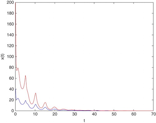
Figure 2. An example of solution to Equation (7(7) $\frac{\mathrm{d}x}{\mathrm{d}t}=3\gamma \left(t\right)f\left(x\right(t-\tau \left)\right)-\tilde{\sigma }x\left(t\right),$(7) ) for $\gamma \left(t\right)=5+\cos \left(t\right)+\sin \left(2t\right),\tilde{\sigma }=2,\tau =5,$ and $x_0=40,200$, respectively.

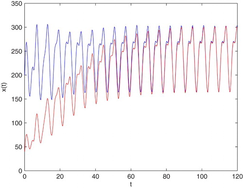
Figure 3. An example of solution to Equation (7(7) $\frac{\mathrm{d}x}{\mathrm{d}t}=3\gamma \left(t\right)f\left(x\right(t-\tau \left)\right)-\tilde{\sigma }x\left(t\right),$(7) ) for $\gamma \left(t\right)=2+{\mathrm{e}}^{\sin \left(\sqrt{2}t\right)},\tilde{\sigma }=2,\tau =5,$ and $x_0=40,200$, respectively.

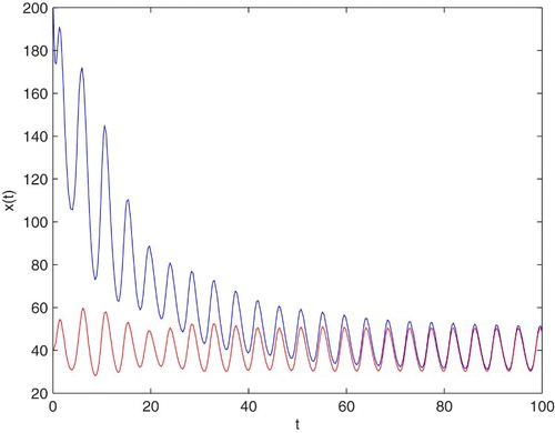
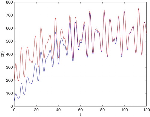
Figure 4. An example of solution to Equation (7(7) $\frac{\mathrm{d}x}{\mathrm{d}t}=3\gamma \left(t\right)f\left(x\right(t-\tau \left)\right)-\tilde{\sigma }x\left(t\right),$(7) ) for $\gamma \left(t\right)=5+\cos \left(t\right)+{\mathrm{e}}^{\sin \left(\sqrt{2}t\right)},\tilde{\sigma }=2,\tau =5,$ and $x_0=40,200$, respectively.

In Figure 1, an example of the behaviour of solutions in the case which is covered by Theorem  2.7(2) is presented. It occurs that, for some values of parameters and any different constant initial values, the tumour will disappear.

In Figures 2–4, three examples of the behaviour of solutions in the case which is covered by Theorem 2.7(1) is presented. It occurs that, for various values of parameters and any different constant initial values, the tumour will tend to the unique almost positive periodic solution.

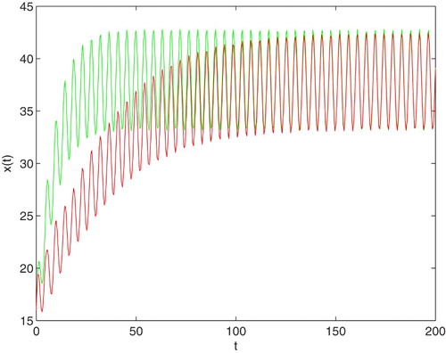
In Figure 5, an example of the behaviour of solutions in the case which is covered by Theorem  3.3(1) is presented (green curve). It occurs that, for some values of parameters and a small constant time delay satisfying the conditions of Theorem 3.3(1), the solution of Equation (7(7) $\frac{\mathrm{d}x}{\mathrm{d}t}=3\gamma \left(t\right)f\left(x\right(t-\tau \left)\right)-\tilde{\sigma }x\left(t\right),$(7) ) will tend to the unique almost positive periodic solution in exponential speed. And for the same values of parameters as that of the red curve, but with a large constant time delay which does not meet the conditions of Theorem 3.3(1), the tumour also will tend to the unique almost positive periodic solution (red curve). The speed of the convergence of the red curve is slower than that of the green curve.

Figure 5. An example of solution to Equation (7(7) $\frac{\mathrm{d}x}{\mathrm{d}t}=3\gamma \left(t\right)f\left(x\right(t-\tau \left)\right)-\tilde{\sigma }x\left(t\right),$(7) ) for $\gamma \left(t\right)=1.6+0.4\ast {\mathrm{e}}^{\cos \left(\sqrt{2}t\right)},\tilde{\sigma }=1,x_0=16$ and $\tau =0.5,5$, respectively.

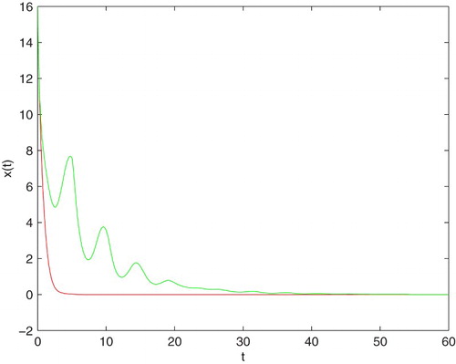
In Figure 6, an example of the behaviour of solutions in the case which is covered by Theorem  3.3(2) is presented (red curve). It occurs that, for some values of parameters and a small constant time delay satisfying the conditions of Theorem 3.3(1), the radius of the tumour will tend to zero in exponential speed. And for the same values of parameters as that of the red curve, but with a large constant time delay which does not meet the conditions of Theorem 3.3(1), the radius of the tumour also will tends to zero (green curve). The speed of the convergence of the green curve is slower than that of the red curve.

Figure 6. An example of solution to Equation (7(7) $\frac{\mathrm{d}x}{\mathrm{d}t}=3\gamma \left(t\right)f\left(x\right(t-\tau \left)\right)-\tilde{\sigma }x\left(t\right),$(7) ) for $\gamma \left(t\right)=1.6+0.4\ast {\mathrm{e}}^{\cos \left(\sqrt{2}t\right)},\tilde{\sigma }=3,x_0=16$ and $\tau =0.1,5$, respectively.

Disclosure statement

No potential conflict of interest was reported by the author(s).

Additional information

Funding

This work of the first two authors is partially supported by NNSF of China (grant nos. 11301474 and 11171295), Foundation for Distinguished Young Teachers in Higher Education of Guangdong, China (grant nos. Yq2013163 and YQ2015167) and NSF of Guangdong Province (grant no. 2015A030313707). The third author is partially supported in part by NNSF of China (grant nos. 51508319, 61374195 and 51409157) and the Nature and Science Fund from Zhejiang Province Ministry of Education (grant no. Y201327642).

References

- M. Bodnar, The nonnegativity of solutions of delay differential equations, Appl. Math. Lett. 13 (2000), pp. 91–95. doi: 10.1016/S0893-9659(00)00061-6
- M. Bodnar and U. Forys, Time delay in necrotic core formation, Math. Biosci. Eng. 2 (2005), pp. 461–472. doi: 10.3934/mbe.2005.2.461
- H. Bohr, Almost Periodic Functions, Chelsea, New York, 1947.
- H. Byrne, The effect of time delays on the dynamics of avascular tumor growth, Math. Biosci. 144 (1997), pp. 83–117. doi: 10.1016/S0025-5564(97)00023-0
- H. Byrne and M. Chaplain, Growth of nonnecrotic tumors in the presence and absence of inhibitors, Math. Biosci. 130 (1995), pp. 151–181. doi: 10.1016/0025-5564(94)00117-3
- H. Byrne and M. Chaplain, Growth of necrotic tumors in the presence and absence of inhibitors, Math. Biosci. 135 (1996), pp. 187–216. doi: 10.1016/0025-5564(96)00023-5
- C. Corduneanu, Almost Periodic Functions, 2nd ed., Chelsea, New York, 1989.
- S. Cui, Analysis of a free boundary problem modeling tumor growth, Acta Math. Sin. 21 (2005), pp. 1071–1082. doi: 10.1007/s10114-004-0483-3
- S. Cui, Fromation of necrotic cores in the growth of tumors: Analytic results, Acta Math. Scientia. 26B (2006), pp. 781–796. doi: 10.1016/S0252-9602(06)60104-5
- S. Cui and A. Friedman, Analysis of a mathematical model of the effect of inhibitors on the growth of tumors, Math. Biosci. 164 (2000), pp. 103–137. doi: 10.1016/S0025-5564(99)00063-2
- S. Cui and S. Xu, Analysis of mathematical models for the growth of tumors with time delays in cell proliferation, J. Math. Anal. Appl. 336 (2007), pp. 523–541. doi: 10.1016/j.jmaa.2007.02.047
- H. Ding and J. Nieto, A new approach for positive almost periodic solutions to a class of Nicholson's blowflies model, J. Comput. Appl. Math. 253 (2013), pp. 249–254. doi: 10.1016/j.cam.2013.04.028
- H. Ding, T. Xiao, and J. Liang, Existence of positive almost automorphic solutions to nonlinear delay integral equations, Nonlinear Anal. TMA. 70 (2009), pp. 2216–2231. doi: 10.1016/j.na.2008.03.001
- A.M. Fink, Almost Periodic Differential Equations, Lecture Notes in Mathematics, Vol. 377, Springer, Berlin, 1974.
- J. Folkman, Self-regulation of growth in three dimensions, J. Exp. Med. 138 (1973), pp. 262–284. doi: 10.1084/jem.138.4.745
- U. Forýs and M. Bodnar, Time delays in proliferation process for solid avascular tumour, Math. Comput. Model. 37 (2003), pp. 1201–1209. doi: 10.1016/S0895-7177(03)80019-5
- U. Forýs and M. Bodnar, Time delays in regulatory apoptosis for solid avascular tumour, Math. Comput. Model. 37 (2003), pp. 1211–1220. doi: 10.1016/S0895-7177(03)00131-6
- U. Forýs and A. Mokwa-Borkowska, Solid tumour growth analysis of necrotic core formation, Math. Comput. Model. 42 (2005), pp. 593–600. doi: 10.1016/j.mcm.2004.06.022
- A. Friedman and F. Reitich, Analysis of a mathematical model for the growth of tumors, J. Math. Biol. 38 (1999), pp. 262–284. doi: 10.1007/s002850050149
- D. Guo and V. Lakshmikantham, Nonlinear Problems in Abstract Cones, Academic Press, New York, 1988.
- R.R. Sarkar and S. Banerjee, A time delay model for control of malignant tumor growth, National Conference on Nonlinear Systems and Dynamics, CTS, I.I.T. Kharagpur, 2006, 1–4.
- D.R. Smart, Fixed Points Theorems, Cambridge University Press, Cambridge, 1980.
- S. Xu, Analysis of tumor growth under direct effect of inhibitors with time delays in proliferation, Nonlinear Anal. Real World Appl. 11 (2010), pp. 401–406. doi: 10.1016/j.nonrwa.2008.11.002
- S. Xu, Analysis of a delayed free boundary problem for tumor growth, Discret. Contin. Dyn. Syst. B. 18 (2011), pp. 293–308.
- S. Xu, M. Bai, and X.Q. Zhao, Analysis of a solid avascular tumor growth model with time delays in proliferation process, J. Math. Anal. Appl. 391 (2012), pp. 38–47. doi: 10.1016/j.jmaa.2012.02.034
- S. Xu, Analysis of a free boundary problem for tumor growth in a periodic external environment, Bound Value Probl. 2015 (2015), pp. 1–12. doi: 10.1186/s13661-014-0259-3