Discrete stochastic analogs of Erlang epidemic models

ABSTRACT

Erlang differential equation models of epidemic processes provide more realistic disease-class transition dynamics from susceptible (S) to exposed (E) to infectious (I) and removed (R) categories than the ubiquitous SEIR model. The latter is itself is at one end of the spectrum of Erlang SE${}_m$I${}_n$R models with $m\ge 1$ concatenated E compartments and $n\ge 1$ concatenated I compartments. Discrete-time models, however, are computationally much simpler to simulate and fit to epidemic outbreak data than continuous-time differential equations, and are also much more readily extended to include demographic and other types of stochasticity. Here we formulate discrete-time deterministic analogs of the Erlang models, and their stochastic extension, based on a time-to-go distributional principle. Depending on which distributions are used (e.g. discretized Erlang, Gamma, Beta, or Uniform distributions), we demonstrate that our formulation represents both a discretization of Erlang epidemic models and generalizations thereof. We consider the challenges of fitting SE${}_m$I${}_n$R models and our discrete-time analog to data (the recent outbreak of Ebola in Liberia). We demonstrate that the latter performs much better than the former; although confining fits to strict SEIR formulations reduces the numerical challenges, but sacrifices best-fit likelihood scores by at least 7%.

KEYWORDS:

• Distributed-delay
• Boxcar models
• discrete-time models
• Ebola
• gamma distributed waiting times

AMS SUBJECT CLASSIFICATION:

• 92D30

Introduction

An SEIR epidemic modelling framework, where S, E, I and R represent the named susceptible (S), exposed (E: infected but not yet infectious), infectious (I), and removed (R: either dead or recovered and now immune) disease classes – and italicized letters S, E, I, and R represent the number of individuals in each of these classes – underpins all infectious disease modelling at the population level [27,52]. This holds whether the models are continuous or discrete-time [21], deterministic or stochastic [2,10], or framed at the compartmental- or individual-level formulation [1,11,24]. Fitting epidemiological models to real data possess significant challenges because most epidemics do not conform to the assumptions underlying the basic SEIR formulation. In particular, populations are rarely spatially homogeneous [25,30,32], and disease transmission varies with age [55] and other individual-level factors, including behaviour [16]. An additional acknowledged weaknesses of the SEIR formulation is that if a group of n individuals enter class X (X = E or I) at time t and exit at rate γ, then the number of individuals still in state X at time $t+\tau$ is given by the exponential function $n(t+\tau )=n\left(t\right){\mathrm{e}}^{-{\gamma }^{\mathrm{X}}\tau }$ [56]. This approach has been shown from outbreak data to underestimate the basic reproductive ratio ${\mathcal{R}}_0$ of an epidemic process [56]. A more reasonable assumption is that individuals will mostly exit around a characteristic disease-class-specific residence time ${\rho }^{\mathrm{X}}$, which corresponds to the latent period and infectious period for any disease [49,56]. Models that address deviations from the above assumptions have been proposed. For example, one way to modify the standard SEIR continuous-time formulation so that the modal exit-time of individuals from disease states E and I is close to empirically measured values, ${\rho }^{\mathrm{E}}$ and ${\rho }^{\mathrm{I}}$ respectively, is to use either a discrete-time formulation in which individuals take a set number of time periods to move through each disease state (e.g. as has been done in modelling SARS [23,37]), or to use a continuous time distributed-delay approach [7,9,13,33]. This latter approach can be modelled using a so-called boxcar formulation: the process by which individuals pass through each disease state (i.e. compartment) X is represented by individuals passing through $k^{\mathrm{X}}$ concatenated sub-compartments at a rate ${\gamma }^{\mathrm{X}}$ in each of the sub-compartments [7,31,33,35] (Figure 1). In this case, the number of individuals $n\left(t\right)$ entering at time t still in state X at time $t+\tau$ is not given by an exponential function, but rather $n\left(t\right)$ multiplied by $(1-F_{\mathrm{Erlang}}(\tau ,k^{\mathrm{X}},{\gamma }^{\mathrm{X}}\left)\right)$, where $F_{\mathrm{Erlang}}(\tau ,k^{\mathrm{X}},{\gamma }^{\mathrm{X}})$ is the cumulative Erlang distribution with parameters $k^{\mathrm{X}}$ and ${\gamma }^{\mathrm{X}}$. Note that the Erlang is a special case of the Gamma distribution when the shape parameter $k^{\mathrm{X}}$ is a positive integer [33]. Further, the fact that a distributed-delay integrodifferential equation formulation can, under certain assumptions, be turned into an ordinary differential equation formulation of higher dimension, using the so-called ‘linear chain trick’ has been known in biological modelling for the past 40 years ([14,40,44], and see [51] for a more recent treatment).

Figure 1. The standard continuous-time SEIR compartmental model has individuals flowing through the E and I compartments at rates ${\gamma }^{\mathrm{E}}$ and ${\gamma }^{\mathrm{I}}$ respectively, with rates of flow from compartments S to E and V to S (V is the immune part of R, D is the dead part of R) represented by τ and ${\gamma }^{\mathrm{V}}$ respectively. The boxcar or Erlang version divides E into $k^{\mathrm{E}}$ and I into $k^{\mathrm{I}}$ sub-compartments with the mean time that it takes to pass through compartments E and I now given by ${\rho }^{\mathrm{E}}=k^{\mathrm{E}}/{\gamma }^{\mathrm{E}}$ and ${\rho }^{\mathrm{I}}=k^{\mathrm{I}}/{\gamma }^{\mathrm{I}}$, respectively. The discrete time-to-go model can be regarded as the discrete-time analog of the Erlang model where the proportions (deterministic setting) or probabilities (stochastic setting) $p_i^{\mathrm{E}}$, $i=1,\dots ,n^{\mathrm{E}}$ and $p_j^{\mathrm{I}}$, $j=1,\dots ,n^{\mathrm{I}}$ follow Erlang distributions, as described in the text.

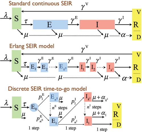
Beyond individuals emerging from a disease state according to an Erlang distribution, a more general discrete-time modelling approach can be taken in which any distribution of emergence can be specified. Here we develop a general discrete-time, distributed-delay formulation, taking the novel approach of identifying disease subclasses that represent the number of days individuals have left before they transfer from the current disease class to the next in the chain (i.e. E to I and I to R, and so on), as depicted in Figure 1. This permits exponential, Erlang, and Uniform distributions, among others, to be used. Beyond comparing our discrete-time formulation that corresponds to continuous-time Erlang formulations, we compare simulation output among the Erlang, Exponential, and Uniform cases, demonstrating some surprising results. For example, the case that yields the highest levels of prevalence switches as the values of the reproductive ratios ${\mathcal{R}}_0$ increase from low (${\mathcal{R}}_0=1.25$) to very high (${\mathcal{R}}_0=20$). We also demonstrate how easily discrete-time formulations can be implemented stochastically, and we compare sample mean ensembles of stochastic simulations to discrete-time solutions. Finally, we compare the efficiencies of fitting continuous-time Erlang models and our various discrete models to real data. To keep our analysis focused, our formulation and simulations ignore the processes of recruitment and mortality. These, of course, are easily added, as we discuss, along with other important extensions such as spatial structure using metapopulation networks.

Model formulation

Continuous deterministic

The basic equations for the SEIR distributed-delay model [7] are well known. For the sake of completeness, however, we present these equations here in terms of a general transmission function $\mathcal{T})$ that depends on the total number $I_{\mathrm{tot}}$ of infectious individuals in the population. As depicted in Figure 1, if the number of E and I class compartments is $k^{\mathrm{E}}$ and $k^{\mathrm{I}}$, respectively, with associated rate parameters ${\gamma }^{\mathrm{E}}$ and ${\gamma }^{\mathrm{I}}$, then the boxcar models takes the form: (1) $\begin{array}{rl}\frac{\mathrm{d}S}{\mathrm{d}t}& =-\mathcal{T}\left(I_{\mathrm{tot}}\right)S\\ \frac{\mathrm{d}{E}_1}{\mathrm{d}t}& =\mathcal{T}\left(I_{\mathrm{tot}}\right)S-{\gamma }^{\mathrm{E}}{E}_1\\ \frac{\mathrm{d}{E}_2}{\mathrm{d}t}& ={\gamma }^{\mathrm{E}}(E_1-E_2)\\ & ⋮\\ \frac{\mathrm{d}{E}_{k^{\mathrm{E}}}}{\mathrm{d}t}& ={\gamma }^{\mathrm{E}}(E_{k^{\mathrm{E}}-1}-E_{k^{\mathrm{E}}})\\ \frac{\mathrm{d}{I}_1}{\mathrm{d}t}& ={\gamma }^{\mathrm{E}}{E}_{k^{\mathrm{E}}}-{\gamma }^{\mathrm{I}}{I}_1\\ \frac{\mathrm{d}{I}_2}{\mathrm{d}t}& ={\gamma }^{\mathrm{I}}(I_1-I_2)\\ & ⋮\\ \frac{\mathrm{d}{I}_{k^{\mathrm{I}}}}{\mathrm{d}t}& ={\gamma }^{\mathrm{I}}(I_{k^{\mathrm{I}}-1}-I_{k^{\mathrm{I}}})\\ \frac{\mathrm{d}R}{\mathrm{d}t}& ={\gamma }^{\mathrm{I}}{I}_{k^{\mathrm{I}}},\end{array}$(1) where (2) $E_{\mathrm{tot}}=\sum _{i=1}^{k_{\mathrm{E}}}{E}_i\text{and}{I}_{\mathrm{tot}}=\sum _{i=1}^{k_{\mathrm{I}}}{I}_i.$(2) The simplest form of the transmission function is $\mathcal{T}\left(I\right)=\mathcal{T}\left(I_{\mathrm{tot}}\right)=\beta I_{\mathrm{tot}}$. It is convenient when applying the model to normalize the transmission rate parameter $\beta >0$ in $\mathcal{T}$ by total population size N so that β does not have to be adjusted for populations of different sizes. This ensures that expressions for the basic reproductive ratio, ${\mathcal{R}}_0$, of the disease is independent of population size (cf. [4]). This normalization is done by dividing β by N, where (3) $N\left(t\right)=S\left(t\right)+E_{\mathrm{tot}}\left(t\right)+I_{\mathrm{tot}}\left(t\right)+R\left(t\right).$(3) If deaths are ignored during the course of the epidemic, then $N\left(t\right)$ is constant and the transmission function (4) $\mathcal{T}\left(I_{\mathrm{tot}}\right)\left(t\right)=\frac{\beta I_{\mathrm{tot}}\left(t\right)}{N},$(4) varies only with $I_{\mathrm{tot}}\left(t\right)$ over time, otherwise it will vary with $N\left(t\right)$ as well. In this latter case, $\mathcal{T}\left(I_{\mathrm{tot}}\right)\left(t\right)$ is referred to as frequency-dependent transmission. This representation of transmission is particularly appropriate when contact rates are influenced by processes other than population density, as in sexually transmitted diseases [22]. The ubiquitous density-dependent form $\tau (I,N)=\beta I$ though is useful when population density is low. A more general approach that approximates density-dependent transmission at relatively low populations densities and frequency-dependent transmission at relatively high population densities, for some arbitrary constant L>0 (to be estimated when fitting the model to data), is given by the transmission function [21,41] $\tau (I,N)=\beta I/(N+L)$.

The assumption that the transmission rate parameter β is time independent is also problematic. The primary reason that epidemics subside, other than running out of susceptible individuals (which is linked to the so-called threshold effect [22,38]), is that $\beta \left(t\right)$ precipitously falls due to behavioural changes that influence contact rates as the epidemic proceeds (e.g. as in the recent Ebola outbreak in West Africa [12,24]). A remedy for this is to assume that β has the exponential form $\beta \left(t\right)={\beta }_0{\mathrm{e}}^{-\epsilon t}$ (e.g. as in [3]). This approach, however, implies that β declines most steeply at the start of the epidemic – a highly suspect assumption. A more likely situation is that β only starts to decline once public awareness of the full potential of the epidemic becomes apparent. In this case, a reverse S-shaped curve, such as (5) $\beta \left(t\right)=\frac{{\beta }_0}{1+{\left(\frac{t}{t_{\mathrm{c}}}\right)}^{\epsilon }},$(5) is more realistic, where $t_{\mathrm{c}}>0$ is that amount of time after the start of the epidemic that it takes for $\beta \left(t\right)$ to fall to half its original intensity, and $\epsilon >1$ is an abruptness parameter for the onset of this fall (in a manner analogous to the onset of density-dependence discussed in [20]). In the absence of an independent estimate for $t_{\mathrm{c}}$ when fitting models to data, one can estimate ${\beta }_0$ by fitting a constant β model to the early stages of an epidemic, and then use this value to estimate the reproductive ratio parameter ${\mathcal{R}}_0$ (the number of individuals that the index case can be expected to infect at the start of the epidemic [15,26]).

Using the simple frequency-dependent transmission rate (Equation (4(4) $\mathcal{T}\left(I_{\mathrm{tot}}\right)\left(t\right)=\frac{\beta I_{\mathrm{tot}}\left(t\right)}{N},$(4) )) and assuming that β is constant over time, the model given by Equations (1(1) $\begin{array}{rl}\frac{\mathrm{d}S}{\mathrm{d}t}& =-\mathcal{T}\left(I_{\mathrm{tot}}\right)S\\ \frac{\mathrm{d}{E}_1}{\mathrm{d}t}& =\mathcal{T}\left(I_{\mathrm{tot}}\right)S-{\gamma }^{\mathrm{E}}{E}_1\\ \frac{\mathrm{d}{E}_2}{\mathrm{d}t}& ={\gamma }^{\mathrm{E}}(E_1-E_2)\\ & ⋮\\ \frac{\mathrm{d}{E}_{k^{\mathrm{E}}}}{\mathrm{d}t}& ={\gamma }^{\mathrm{E}}(E_{k^{\mathrm{E}}-1}-E_{k^{\mathrm{E}}})\\ \frac{\mathrm{d}{I}_1}{\mathrm{d}t}& ={\gamma }^{\mathrm{E}}{E}_{k^{\mathrm{E}}}-{\gamma }^{\mathrm{I}}{I}_1\\ \frac{\mathrm{d}{I}_2}{\mathrm{d}t}& ={\gamma }^{\mathrm{I}}(I_1-I_2)\\ & ⋮\\ \frac{\mathrm{d}{I}_{k^{\mathrm{I}}}}{\mathrm{d}t}& ={\gamma }^{\mathrm{I}}(I_{k^{\mathrm{I}}-1}-I_{k^{\mathrm{I}}})\\ \frac{\mathrm{d}R}{\mathrm{d}t}& ={\gamma }^{\mathrm{I}}{I}_{k^{\mathrm{I}}},\end{array}$(1) )–(4(4) $\mathcal{T}\left(I_{\mathrm{tot}}\right)\left(t\right)=\frac{\beta I_{\mathrm{tot}}\left(t\right)}{N},$(4) ) is a five parameter system ($\beta >0$, ${\gamma }^{\mathrm{E}}>0$, and ${\gamma }^{\mathrm{I}}>0$, as well as positive integers $k^{\mathrm{E}}$ and $k^{\mathrm{I}}$) that can be fitted to data to obtain the best estimate of the transmission rate parameter β, and the mean residence times (6) ${\rho }^{\mathrm{E}}=\frac{k^{\mathrm{E}}}{{\gamma }^{\mathrm{E}}}\text{and}{\rho }^{\mathrm{I}}=\frac{k^{\mathrm{I}}}{{\gamma }^{\mathrm{I}}},$(6) in the disease states E and I, respectively. This also implies that the mean residence from exposure to removal is (7) ${\rho }^{\mathrm{E}+\mathrm{I}}=\frac{k^{\mathrm{E}}}{{\gamma }^{\mathrm{E}}}+\frac{k^{\mathrm{I}}}{{\gamma }^{\mathrm{I}}}.$(7) Here we make use of the fundamental definition of ${\mathcal{R}}_0$ as the ratio of all newly infected individuals transferring into disease classes E+I to the net change of individuals across classes E+I [15,26]. This is formally equivalent to finding the dominant eigenvalue of the next generation matrix, as defined in [53]. Since we are ignoring births and deaths, this ratio has the particularly simple form ${\mathcal{R}}_0=\beta {\rho }^{\mathrm{I}}=\frac{\beta k^{\mathrm{I}}}{{\gamma }^{\mathrm{I}}}.$ Note that ignoring births and deaths can also be regarded as an approximation to situations where the epidemiological process is an order of magnitude faster than demographic processes. This is, however, an assumption that breaks down once disease-induced mortality rates become significantly greater than background natural mortality rates.

Discrete time-to-go formulation

In formulating a discrete-time analogue of Equation (1(1) $\begin{array}{rl}\frac{\mathrm{d}S}{\mathrm{d}t}& =-\mathcal{T}\left(I_{\mathrm{tot}}\right)S\\ \frac{\mathrm{d}{E}_1}{\mathrm{d}t}& =\mathcal{T}\left(I_{\mathrm{tot}}\right)S-{\gamma }^{\mathrm{E}}{E}_1\\ \frac{\mathrm{d}{E}_2}{\mathrm{d}t}& ={\gamma }^{\mathrm{E}}(E_1-E_2)\\ & ⋮\\ \frac{\mathrm{d}{E}_{k^{\mathrm{E}}}}{\mathrm{d}t}& ={\gamma }^{\mathrm{E}}(E_{k^{\mathrm{E}}-1}-E_{k^{\mathrm{E}}})\\ \frac{\mathrm{d}{I}_1}{\mathrm{d}t}& ={\gamma }^{\mathrm{E}}{E}_{k^{\mathrm{E}}}-{\gamma }^{\mathrm{I}}{I}_1\\ \frac{\mathrm{d}{I}_2}{\mathrm{d}t}& ={\gamma }^{\mathrm{I}}(I_1-I_2)\\ & ⋮\\ \frac{\mathrm{d}{I}_{k^{\mathrm{I}}}}{\mathrm{d}t}& ={\gamma }^{\mathrm{I}}(I_{k^{\mathrm{I}}-1}-I_{k^{\mathrm{I}}})\\ \frac{\mathrm{d}R}{\mathrm{d}t}& ={\gamma }^{\mathrm{I}}{I}_{k^{\mathrm{I}}},\end{array}$(1) ), we take an approach of placing individuals into subclasses that represent the length of time that each will remain within the disease class under consideration. Thus, we use the notation $E_i(t+1)$ to represent the number of individuals in disease class E at time t+1 who will depart from this class (to enter class I) at time t+1+i. These individuals were either in compartment $E_{i+1}$ at time t or are newly allocated from the individuals that were infected over the time interval $[t,t+1)$ using the proportions described below. The same process applies to the compartments represented by the variables $I_i(t+1)$, with individuals transitioning to disease class R. These proportions are denoted by $0<p_i^{\mathrm{E}}<1$, $i=1,\dots ,n^{\mathrm{E}}$ and $0<p_i^{\mathrm{I}}<1$, $i=1,\dots ,n^{\mathrm{I}}$, and represent the proportions of individuals entering the disease classes E and I who only stay in those classes for i additional periods of time. The integers $n^{\mathrm{E}}$ and $n^{\mathrm{I}}$ are selected so that all individuals (essentially $>99\mathrm{\%}$ in the case of populations of several thousand or more individuals) upon entering diseases classes E and I at time t have exited these disease classes on or before times $t+n^{\mathrm{E}}$ and $t+n^{\mathrm{I}}$, respectively. In the context of stochastic models, these proportions can be used to characterize the cumulative functions $F(x;k^{\mathrm{E}},{\gamma }^{\mathrm{E}})$ and $F(x;k^{\mathrm{I}},{\gamma }^{\mathrm{I}})$ of two distributions: namely, $\begin{array}{rl}F(0;k^{\mathrm{X}},{\gamma }^{\mathrm{X}})& =0,F(j;k^{\mathrm{X}},{\gamma }^{\mathrm{X}})=\sum _{i=1}^j{p}_i^{\mathrm{X}},j=1,\dots ,n^{\mathrm{X}},\\ F(n^{\mathrm{X}};k^{\mathrm{X}},{\gamma }^{\mathrm{X}})& =1,\mathrm{X}=\mathrm{E},\mathrm{I}.\end{array}$ In our discrete model, we use the variables $E_0\left(t\right)$ and $I_0\left(t\right)$ to represent the number of individuals changing state over the discrete-time interval $[t,t+1]$ from S to E and E to I, respectively. We also use $E_{\mathrm{tot}}\left(t\right)$ and $I_{\mathrm{tot}}\left(t\right)$ to represent the total number of individuals in classes E and I at time t. Over the time interval $[t,t+1)$, the susceptibles $S\left(t\right)$ are assumed to be exposed to $I_{\mathrm{tot}}\left(t\right)$ infectious individuals (taken to be constant over the interval, which is generally a reasonable approximation), thereby resulting in the infection of approximately (8) $E_0\left(t\right)=\left(1-{\mathrm{e}}^{-\mathcal{T}\left(I_{\mathrm{tot}}(t-i)\right)}\right)S\left(t\right),$(8) susceptible individuals. Hence we obtain the equation: (9) $S(t+1)=S\left(t\right)-E_0.$(9) Recall that the equations for the compartments $E_i(t+1)$ need to account for the transfer of individuals from $E_{i+1}\left(t\right)$, as well as the newly allocated individuals $p_{i+1}^{\mathrm{E}}{E}_0\left(t\right)$. These considerations yield the system: (10) $\begin{array}{rl}{E}_{n^{\mathrm{E}}}(t+1)& =p_{n^{\mathrm{E}}}^{\mathrm{E}}{E}_0\\ E_{n^{\mathrm{E}}-1}(t+1)& =E_{n^{\mathrm{E}}}\left(t\right)+p_{n^{\mathrm{E}}-1}^{\mathrm{E}}{E}_0\\ & ⋮\\ E_1(t+1)& =E_2\left(t\right)+p_1^{\mathrm{E}}{E}_0.\end{array}$(10) These newly infectious individuals $I_0\left(t\right)$ can themselves be distributed so that proportions $p_i^{\mathrm{I}}$, where $i=1,\dots ,n^{\mathrm{I}}$ enter the removed class at time t. That is, we obtain the equations: (11) $\begin{array}{rl}{I}_{n^{\mathrm{I}}}(t+1)& =p_{n^{\mathrm{I}}}^{\mathrm{I}}{E}_1\left(t\right),\\ I_{n^{\mathrm{I}}-1}(t+1)& =I_{n^{\mathrm{I}}}\left(t\right)+p_{n^{\mathrm{I}}-1}^{\mathrm{I}}{E}_1\left(t\right)\\ & ⋮\\ I_1(t+1)& =I_2\left(t\right)+p_1^{\mathrm{I}}{E}_1\left(t\right),\\ R(t+1)& =R\left(t\right)+I_1\left(t\right).\end{array}$(11) Finally, we need to compute $E_{\mathrm{tot}}\left(t\right)$ and $I_{\mathrm{tot}}\left(t\right)$ by applying Equation (2(2) $E_{\mathrm{tot}}=\sum _{i=1}^{k_{\mathrm{E}}}{E}_i\text{and}{I}_{\mathrm{tot}}=\sum _{i=1}^{k_{\mathrm{I}}}{I}_i.$(2) ) with $n^{\mathrm{E}}$ and $n^{\mathrm{I}}$ replacing $k^{\mathrm{E}}$ and $k^{\mathrm{I}}$ to obtain (12) $E_{\mathrm{tot}}\left(t\right)=\sum _{i=1}^{n^{\mathrm{E}}}{E}_i\left(t\right)\left)\text{and}{I}_{\mathrm{tot}}\right(t)=\sum _{i=1}^{n^{\mathrm{I}}}{I}_i(t\left)\right).$(12)

Stochastic implementation

The discrete stochastic formulation results in a model that is identical to the discrete deterministic model except for the fact that proportions in Equations (10(10) $\begin{array}{rl}{E}_{n^{\mathrm{E}}}(t+1)& =p_{n^{\mathrm{E}}}^{\mathrm{E}}{E}_0\\ E_{n^{\mathrm{E}}-1}(t+1)& =E_{n^{\mathrm{E}}}\left(t\right)+p_{n^{\mathrm{E}}-1}^{\mathrm{E}}{E}_0\\ & ⋮\\ E_1(t+1)& =E_2\left(t\right)+p_1^{\mathrm{E}}{E}_0.\end{array}$(10) ) and (11(11) $\begin{array}{rl}{I}_{n^{\mathrm{I}}}(t+1)& =p_{n^{\mathrm{I}}}^{\mathrm{I}}{E}_1\left(t\right),\\ I_{n^{\mathrm{I}}-1}(t+1)& =I_{n^{\mathrm{I}}}\left(t\right)+p_{n^{\mathrm{I}}-1}^{\mathrm{I}}{E}_1\left(t\right)\\ & ⋮\\ I_1(t+1)& =I_2\left(t\right)+p_1^{\mathrm{I}}{E}_1\left(t\right),\\ R(t+1)& =R\left(t\right)+I_1\left(t\right).\end{array}$(11) ) are replaced by random drawings from multinomial distributions, which approach proportions (i.e. the discrete formulation) as ${\mathcal{R}}_0$ (i.e. β) increases in size and the number of samples grows large. In presenting the stochastic model, we use the notation $x\sim \mathrm{BINOMIAL}\left[n,p\right],$ to denote that x is a random variable representing the number of heads that might be obtained when flipping a biased coin n times, with a probability p of getting heads on each flip (i.e. a Bernoulli process with probability p). Thus, x is binomially distributed. We will use the notation X to represent an instance of the number of heads (positive outcomes) of an actual n-trial sampling of this distribution with probability parameter p. More generally: $({\hat{X}}_1,\dots ,{\hat{X}}_q)\text{is one instance of}(x_1,\dots ,x_q)\sim \mathrm{MULTINOMIAL}\left[n,p_1,\dots ,p_q\right].$ In other words, it is the probability of getting ${\hat{X}}_i$ positive outcomes of type $i=1,\dots ,q$ when the probability of getting a positive outcome of type i at any drawing is $p_i$, with $\sum _{i=1}^q{p}_i=1$, and the total number of drawings is n. To keep our presentation succinct, the convention $({\hat{X}}_1,\dots ,{\hat{X}}_q):=\mathrm{MULTINOMIAL}\left[n,p_1,\dots ,p_q\right],$ is adopted in the model formulations below to denote one outcome of a random drawing from the indicated distribution.

With this above notation, the stochastic equivalent of the deterministic model represented by Equations (9(9) $S(t+1)=S\left(t\right)-E_0.$(9) )–(12(12) $E_{\mathrm{tot}}\left(t\right)=\sum _{i=1}^{n^{\mathrm{E}}}{E}_i\left(t\right)\left)\text{and}{I}_{\mathrm{tot}}\right(t)=\sum _{i=1}^{n^{\mathrm{I}}}{I}_i(t\left)\right).$(12) ) is (13) $\begin{array}{rl}{I}_{\mathrm{tot}}\left(t\right)& =\sum _{i=1}^{n^{\mathrm{I}}}{I}_i\left(t\right))\\ {\hat{E}}_0\left(t\right)& =\mathrm{BINOMIAL}\left[S\left(t\right),1-{\mathrm{e}}^{-\mathcal{T}\left(I_{\mathrm{tot}}(t-i)\right)}\right]\\ \left({\hat{E}}_1\left(t\right),\dots ,{\hat{E}}_{n^{\mathrm{E}}}\left(t\right)\right)& :=\mathrm{MULTINOMIAL}\left[E_0\left(t\right);p_1^{\mathrm{E}},\dots ,p_{n^{\mathrm{E}}}^{\mathrm{E}}\right]\\ S(t+1)& =S\left(t\right)-E_0\left(t\right)\\ E_{n^{\mathrm{E}}-1}(t+1)& ={\hat{E}}_{n^{\mathrm{E}}}\left(t\right)\\ E_{n^{\mathrm{E}}-2}(t+1)& =E_{n^{\mathrm{E}}-1}\left(t\right)+{\hat{E}}_{n^{\mathrm{E}}-1}\left(t\right)\\ & ⋮\\ E_1(t+1)& =E_2\left(t\right)+{\hat{E}}_2\left(t\right)\\ I_0(t+1)& =E_1\left(t\right)+{\hat{E}}_1\left(t\right)\\ \left({\hat{I}}_1\left(t\right),\dots ,{\hat{I}}_{n^{\mathrm{E}}}\left(t\right)\right)& :=\mathrm{MULTINOMIAL}\left[I_0\left(t\right);p_1^{\mathrm{I}},\dots ,p_{n^{\mathrm{I}}}^{\mathrm{I}}\right]\\ I_{n^{\mathrm{I}}-1}(t+1)& ={\hat{I}}_{n^{\mathrm{I}}}\left(t\right),\\ I_{n^{\mathrm{I}}-2}(t+1)& =I_{n^{\mathrm{I}}-1}\left(t\right)+{\hat{I}}_{n^{\mathrm{I}}-1}\left(t\right)\\ & ⋮\\ I_1(t+1)& =I_2\left(t\right)+{\hat{I}}_2\left(t\right)\\ R(t+1)& =R\left(t\right)+I_1\left(t\right)+{\hat{I}}_1\left(t\right).\end{array}$(13)

Erlang probabilities

If we want our probabilities to follow truncated Erlang distributions, then we can first select $n^{\mathrm{E}}$ such that $n^{\mathrm{E}}=\underset{n}{\arg \min }\left[C^{\mathrm{E}}\left(n\right)=\sum _{j=1}^{n-1}\frac{{\mathrm{e}}^{n{\gamma }^{\mathrm{E}}}(n{\gamma }^{\mathrm{E}}{)}^j}{(j-1)!}>0.99\right].$ We can then define the probabilities associated with passage through disease class E as $p_i^{\mathrm{E}}=\frac{1}{C^{\mathrm{E}}\left(n^{\mathrm{E}}\right)}\left(\sum _{j=1}^{n^{\mathrm{E}}-1}\frac{{\mathrm{e}}^{(i-1){\gamma }^{\mathrm{E}}}(i{\gamma }^{\mathrm{E}}{)}^j}{(j-1)!}-\sum _{j=1}^{n^{\mathrm{E}}-1}\frac{{\mathrm{e}}^{i{\gamma }^{\mathrm{E}}}(i{\gamma }^{\mathrm{E}}{)}^j}{j!}\right),i=1,\dots ,n^{\mathrm{E}}.$ Similarly, we select $n^{\mathrm{I}}$ such that $n^{\mathrm{I}}=\underset{n}{\arg \min }\left[C^{\mathrm{I}}\left(n\right)=\sum _{j=1}^{n-1}\frac{{\mathrm{e}}^{n{\gamma }^{\mathrm{I}}}(n{\gamma }^{\mathrm{I}}{)}^j}{(j-1)!}>0.99\right]$ and define $p_i^{\mathrm{I}}=\frac{1}{C^{\mathrm{I}}\left(n^{\mathrm{I}}\right)}\left(\sum _{j=1}^{n^{\mathrm{I}}-1}\frac{{\mathrm{e}}^{(i-1){\gamma }^{\mathrm{I}}}(i{\gamma }^{\mathrm{I}}{)}^j}{(j-1)!}-\sum _{j=1}^{n^{\mathrm{I}}-1}\frac{{\mathrm{e}}^{i{\gamma }^{\mathrm{I}}}(i{\gamma }^{\mathrm{I}}{)}^j}{j!}\right),i=1,\dots ,n^{\mathrm{I}}.$ Fitting the discrete Erlang model to data involves estimating five parameters: $(k^{\mathrm{E}},{\gamma }^{\mathrm{E}},k^{\mathrm{I}},{\gamma }^{\mathrm{I}},\beta )$. It also requires constraining $k^{\mathrm{E}}$ and $k^{\mathrm{I}}$ to be positive integers. In general, however, we can allow $k^{\mathrm{E}}$ and $k^{\mathrm{I}}$ to vary continuously on the positive reals, and use gamma functions, which interpolate the Erlang when $k^{\mathrm{E}}$ and $k^{\mathrm{I}}$ are not integers. The boxcar version of the distributed-delay model (which, in addition to its formulation in terms of k first-order differential equations, can also be formulated as a $k\mathrm{th}$ order ordinary differential equation), under assumptions that the rate is constant through all the box cars associated with each disease class, is known to produce Erlang distribution residence times [29]. This implies that the distribution of residence times x is given by the probability density function $f^{\mathrm{Erlang}}(x;k,\gamma )=\frac{{\gamma }^k{x}^{k-1}{\mathrm{e}}^{-\gamma x}}{(k-1)!},$ and, hence, the cumulative distribution function $F^{\mathrm{Erlang}}(x;k,\gamma )=1-\sum _{j=0}^k\frac{(\gamma x{)}^k{\mathrm{e}}^{-\gamma x}}{j!}.$ From these we can calculate the probabilities (proportions in the deterministic model) that individuals entering a k boxcar complex at time t, and exiting this concatenation of cars during the time interval $[t+i-1,t+i]$, is $p_i^{\mathrm{Erlang}}=\left(\sum _{j=1}^k\frac{{\mathrm{e}}^{(i-1)\gamma }{\left((i-1)\gamma \right)}^j}{j!}-\sum _{j=1}^k\frac{{\mathrm{e}}^{i\gamma }(i\gamma {)}^j}{j!}\right),i=1,\dots ,\mathrm{\infty }.$ A theoretically simpler, and computationally faster, approach to fitting the discrete model to data is to use one parameter Uniform distributions $f^{\mathrm{Unif}}(x;0,a)$ rather than two parameter Erlang. These probabilities are provided in the Appendix.

Simulation study

Initial conditions and cases considered

Various approaches can be taken to setting initial conditions in comparing discrete and continuous time simulation models. The primary consideration is to have a good way to match up initial values because the continuous model has $k^{\mathrm{E}}+k^{\mathrm{I}}+2$ states while the discrete model has $n^{\mathrm{E}}+n^{\mathrm{I}}+2$ states (where, typically, $n^{\mathrm{X}}>2k^{\mathrm{X}}$, X=E, I). Further, when injecting stochastic models into the comparative study, one needs to be cognizant of the fact that continuous and discrete deterministic simulations are independent of scale – i.e. the size of N – and only the stochastic simulations are affected by the size of N. Specifically, the influence of demographic stochasticity on simulated values reduces at a rate proportional to $1/\sqrt{N}$. In our first set of simulations, we selected $S\left(0\right)=10,000$, but varied $S\left(0\right)$ from 1000 to ${10}^6$ in subsequent sets of simulations that explore aspects of demographic stochasticity and compare the efficiency of fitting discrete versus continuous models to simulated data. To initiate the start of an epidemic, we placed one individual in the last Esubcomponent class, which corresponds to setting $E_{k^{\mathrm{E}}}\left(0\right)=1$ in the continuous time model and $E_0\left(0\right)=1$ in the discrete-time deterministic and stochastic Erlang models. In all of the simulations, the initial values of the remaining E and I subcomponent states were set to 0, as was $R\left(0\right)$.

For purposes of illustration and comparison of simulations we consider continuous and discrete-time implementations for cases involving $k^{\mathrm{E}}$ and $k^{\mathrm{I}}$ equal to 5 and 10, as well as parameterizations involving ${\gamma }^{\mathrm{E}}$ and ${\gamma }^{\mathrm{I}}$ equal to 0.5, 1, and 2, and β equal to 0.25, 1, and 2, as listed in Table 1. Implementation of these cases by the discrete model requires that we compute probabilities associated with Erlang cumulative distribution functions $F^{\mathrm{Erlang}}(x;5,0.5)$, $F^{\mathrm{Erlang}}(x;5,1)$, $F^{\mathrm{Erlang}}(x;10,1)$, and $F^{\mathrm{Erlang}}(x;10,2)$. These probabilities are given in Table 2.

Table 1. Simulation cases 1–33 are sorted from the shortest (5 days) to longest (10 days) mean infectious period, and then subsorted within infectious periods from shortest to longest total duration (exposed plus infected) and within that from least to most distributed-delay in infected and then exposed.

Cases	$({\gamma }^{\mathrm{E}},k^{\mathrm{E}},{\gamma }^{\mathrm{I}},k^{\mathrm{I}})$	$({\rho }^{\mathrm{E}},{\rho }^{\mathrm{I}},{\rho }^{\mathrm{E}+\mathrm{I}})$	$\beta =0.25$, $\beta =1$, $\beta =2$
1, 17, 33	(1, 5, 1, 5)		${\mathcal{R}}_0=20$
2, 18	(2, 10, 1, 5)
3, 19	(1, 5, 2, 10)	(5, 5, 10)	${\mathcal{R}}_0=1.25$, ${\mathcal{R}}_0=5$
4, 20	(2, 10, 2, 10)
5, 21	(1, 5, 0.5, 5 )
6, 22	(1, 10, 1, 5)
7, 23	(0.5, 5, 2, 10)	(10, 5, 15)	${\mathcal{R}}_0=1.25$, ${\mathcal{R}}_0=5$
8, 24	(1, 10, 2, 10)
9, 25	(1, 5, 0.5, 5)
10, 26	(2, 10, 0.5, 5)
11, 27	(1, 5, 1, 10)	(5, 10, 15)	${\mathcal{R}}_0=2.5$, ${\mathcal{R}}_0=10$
12, 28	(2, 10, 1, 10)
13, 29	(0.5, 5, 0.5, 5)
14, 30	(1, 10, 0.5, 5)
15, 31	(0.5, 5, 1, 10)	(10, 10, 20)	${\mathcal{R}}_0=2.5$, ${\mathcal{R}}_0=10$
16, 32	(1, 10, 1, 10)

Note: Transmission parameter $\beta =0.25$ in Cases 1–16 and $\beta =1$ in Cases 17–32 producing the ${\mathcal{R}}_0$ values given in the last column, while $\beta =2$ was used only in Case 33.

Table 2. Probabilities associated with truncating the four indicated Erlang cumulative distribution functions $F^{\mathrm{Erlang}}(x;k,\gamma )$ ($p_i^{\mathrm{TrEr}}$), as well as the truncated exponential distribution ($p_i^{\mathrm{TrEx}}$: Erlang with k=1): truncation involves setting the $<1\mathrm{\%}$ cumulative right tail probabilities to 0 and renormalizing the remaining $>0.99\mathrm{\%}$ cumulative probabilities to 1.

$(k,\gamma ,\rho )$	$(5,1,5)$	$(10,2,5)$	$(5,0.5,10)$	$(10,1,10)$	$(1,0.2,5)$	$\rho =5$
x=i	$p_i^{\mathrm{TrEr}}$				$p_i^{\mathrm{TrEx}}$	$p_i^{\mathrm{Uni}}$
1	0.0153	0.0004	0.0008	0.0000	0.1828	0.1000
2	0.0902	0.0265	0.0078	0.0002	0.1496	0.1000
3	0.1680	0.1378	0.0238	0.0027	0.1225	0.1000
4	0.1953	0.2482	0.0455	0.0133	0.1003	0.1000
5	0.1755	0.2502	0.0674	0.0365	0.0821	0.1000
6	0.1338	0.1747	0.0848	0.0693	0.0672	0.1000
7	0.0912	0.0947	0.0952	0.1021	0.0551	0.1000
8	0.0573	0.0426	0.0986	0.1249	0.0451	0.1000
9	0.0337	0.0166	0.0958	0.1326	0.0369	0.1000
10	0.0189	0.0058	0.0885	0.1259	0.0302	0.1000
11	0.0102	0.0019	0.0786	0.1093	0.0247	0
12	0.0053	0.0005	0.0675	0.0879	0.0203	0
13	0.0029	0.0001	0.0564	0.0665	0.0166	0
14	0.0013	0	0.0460	0.0477	0.0136	0
15	0.0006	0	0.0368	0.0326	0.0111	0
16	0.0003	0	0.0289	0.0215	0.0091	0
17	0.0001	0	0.0223	0.0136	0.0075	0
18	0.0001	0	0.0170	0.0084	0.0061	0
19	0	0	0.0128	0.0005	0.0050	0
20	0	0	0.0096	0	0.0041	0
21	0	0	0.0070	0	0.0033	0
22	0	0	0.0052	0	0.0027	0
23	0	0	0.0037	0	0.0022	0
24	0	0	0	0	0.0018	0

Note: The last column is the uniform ($p_i^{\mathrm{Uni}}$) distribution for which $\rho =5$.

Differences among continuous deterministic solutions

Continuous-time, deterministic simulations of prevalence levels over time (i.e. plots of $I_{\mathrm{tot}}\left(t\right)$ against t) for Cases 1–32 are illustrated in Figure 2(a). These 32 cases can be organized into four groups, each of which yields the same set of $({\rho }^{\mathrm{E}},{\rho }^{\mathrm{I}},{\rho }^{\mathrm{E}+\mathrm{I}})$ values, differing only in whether 5 or 10 boxcars were used in each of the E and I classes (Table 1). The main difference among the four groups corresponding to a particular set of values $({\hat{\rho }}^{\mathrm{E}},{\hat{\rho }}^{\mathrm{I}},{\hat{\rho }}^{\mathrm{E}+\mathrm{I}})$ is the amount of variation associated with the distributions around ${\rho }^{\mathrm{E}}$ and ${\rho }^{\mathrm{I}}$: specifically, 5-boxcar formulations with associated progression rate $\hat{\gamma }$ have larger variation around ${\rho }^{\mathrm{X}}$ than 10-boxcar formulations with associated rate $2\hat{\gamma }$. These four groups of four cases each were implemented in the context of two values of β to yield corresponding values of the reproductive ratio ${\mathcal{R}}_0$. The resulting eight sets of four cases fall very neatly into eight sets of outputs (Figure 2(a)), indicating that the selection of 5 versus 10-boxcar formulations makes very little difference in terms of the projected levels of disease prevalence associated with a given $(\beta ,{\hat{\rho }}^{\mathrm{E}},{\hat{\rho }}^{\mathrm{I}},{\hat{\rho }}^{\mathrm{E}+\mathrm{I}})$ combination. Clearly, as expected, lower ${\mathcal{R}}_0$ leads to significantly lower peak prevalence, but as we see in Figure 2(a), it also results in longer outbreaks.

Figure 2. A. Disease prevalence values obtained from simulation Cases 1–32 (N= 10,000) of our continuous-time, deterministic SEIR Erlang model are plotted against time. The basic disease reproductive rates (${\mathcal{R}}_0$) and mean residence times in the exposed (${\rho }^{\mathrm{E}}$) and infectious (${\rho }^{\mathrm{E}}$) classes for each of the eight groups of four cases, as detailed in Table 1, are provided for clarity. B. An expanded view (cf. time axis of upper and lower panels) of the four left-most groups of simulations in panel A.

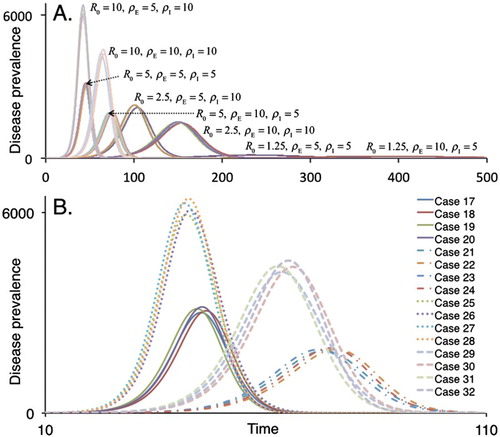
As expected, smaller values of ${\rho }^{\mathrm{E}}$ lead to more rapid outbreaks, as we see in comparing the $({\mathcal{R}}_0,{\hat{\rho }}^{\mathrm{E}},{\hat{\rho }}^{\mathrm{I}})=(10,5,10)$ (cf. Cases 25–28 in Figure 2(b)) and $({\mathcal{R}}_0,{\hat{\rho }}^{\mathrm{E}},{\hat{\rho }}^{\mathrm{I}})=(10,10,10)$ (cf. Cases 29–32 in Figure 2(b)) outbreaks, with a noticeably higher peak prevalence in the former (roughly 6000 versus 4500). Despite these differences, because they arise in delays associated with disease class E only, the areas under the prevalence curves of Cases 25–32 all add up to the same value of 49,651 (units are prevalence-days when time is in days). For Cases 17–24 the area under the prevalence curves sums to 99,995. The pattern of lower-delayed peaks when ${\rho }^{\mathrm{E}}$ is larger, can be verified from Figure 2(a), by comparing the other three sets of comparisons: $({\mathcal{R}}_0,{\hat{\rho }}^{\mathrm{E}},{\hat{\rho }}^{\mathrm{I}})=(5,5,5)$ with $({\mathcal{R}}_0,{\hat{\rho }}^{\mathrm{E}},{\hat{\rho }}^{\mathrm{I}})=(5,10,5)$, $({\mathcal{R}}_0,{\hat{\rho }}^{\mathrm{E}},{\hat{\rho }}^{\mathrm{I}})=(2.5,5,10)$ with $({\mathcal{R}}_0,{\hat{\rho }}^{\mathrm{E}},{\hat{\rho }}^{\mathrm{I}})=(2.5,10,105)$, and $({\mathcal{R}}_0,{\hat{\rho }}^{\mathrm{E}},{\hat{\rho }}^{\mathrm{I}})=(1.25,5,5)$ with $({\mathcal{R}}_0,{\hat{\rho }}^{\mathrm{E}},{\hat{\rho }}^{\mathrm{I}})=(1.25,10,5)$.

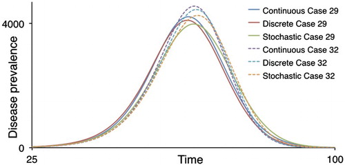
Differences among deterministic and mean stochastic solutions

The discrete Erlang model produces very similar results to its corresponding continuous Erlang model, as we see in Figure 3 for both Cases 29 and 32, although the discrete peak is slightly lower. The mean of the corresponding stochastic ensemble for the case N=10,000 is slightly lower than either deterministic case. Specifically, the [continuous deterministic, discrete deterministic, stochastic mean] peak values for Case 29 are [4219, 4102, 3987] and for Case 32 are [4563, 4450, 4262] (rounding to integers, where the stochastic mean is averaged over 100 Monte Carlo runs).

Figure 3. Disease prevalence values are plotted against time for the continuous and discrete-time, deterministic and the stochastic SEIR Erlang models for Cases 29 and 32, with $\beta =1$, N=10,000, as described in Table 1.

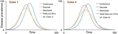
An ensemble of stochastic simulations can be partitioned into two components [42,46,47,50], which we designate here as an initial fadeout (IFO) and breakout (BO) component. Instantiations of the stochastic model that belong to the IFO component, occur with probability $P_{\mathrm{IFO}}$, and those belonging to the BO component occur with probability $1-P_{\mathrm{IFO}}$. It is only the BO component that can be approximately modelled by a corresponding deterministic system [46], provided N is sufficiently large. The size of the IFO component is strongly linked to the critical value ${\mathcal{R}}_0=1$. For ${\mathcal{R}}_0\le 1$ only the IFO component exists, and solutions are referred to as stuttering transmission chains [8,39]. When ${\mathcal{R}}_0>1$, the size of the IFO stuttering transmission chain component rapidly diminishes with increasing ${\mathcal{R}}_0$. For example, in generating the prevalence profiles in Figure 3, which corresponds to the case ${\mathcal{R}}_0=10$ ($\beta =1$), no stuttering chains were evident in our ensemble of 100 runs. Selecting $\beta =0.25$ and repeating the exercise for Runs 1 and 4 for the case N=10,000 – i.e. ${\mathcal{R}}_0=1.25$, we obtained the prevalence profiles plotted in Figure 4. Now, 14 and 9 of the 100 Monte Carlo instantiations for Cases 1 and 4, respectively, were stuttering transmission chains that faded out before they could break out.

Figure 4. Disease prevalence values are plotted against time for the continuous and discrete-time, deterministic models as well as the mean of an ensemble of stochastic SEIR Erlang simulations for Cases 1 and 4 (N=10,000), as described in Table 1. Note that mean of the non-fadeout ensemble is averaged over only those that do not initially fadeout.

IFO rates vary somewhat among repeated sets of ensemble runs and are also affected by the size of the population. In particular, IFO rates are much more difficult to assess in small than in large populations because the sorting of runs into the IFO and BO components is much more difficult when N is relatively small. This problem is evident from the results obtained from simulations conducted for varying N, as reported in the next section.

Small and large populations

When the transmission rate is normalized by the value N, as we have in Equation (4(4) $\mathcal{T}\left(I_{\mathrm{tot}}\right)\left(t\right)=\frac{\beta I_{\mathrm{tot}}\left(t\right)}{N},$(4) ), the solutions to the continuous and discrete deterministic model are scale-independent with regard to population size N. That is, epidemics in isolated towns of 10,000 individuals are per-capita the same as epidemics in isolated mega-cities of 10 million individuals. This is not the case for stochastic populations because demographic stochasticity is not scale-independent. Rather, due to sampling processes for which the variance declines in proportion to sample size, the effects of demographic stochasticity are proportional to $1/\sqrt{N}$. But even large populations are structured into smaller subpopulations that may not be well-mixed on the time scale of an epidemic. This is particularly true of local school populations where the same group of several hundred children aggregate for a substantial portion of the day, on five of the seven days each week. Thus, disease outbreaks in mega-cities, particularly those associated with children, may behave somewhat like disease outbreaks in interconnected sets of large villages or small towns, with large population behaviour depending on suitably high transfer rates of individuals among localities.

To gain insights into the effects of population size, we will consider outbreaks in isolated groups of N=500, 2000, and 50,000 individuals. For the scenario N=500, 90/500 runs (i.e. 18.0%) belonged to the initial fadeout component (IFO), while for the scenarios N=2000 and N=50,000 the IFO contained 21.0% and 18.2% of the runs, respectively.

Discrete model convergence

In Figures 3 and 4, and the third column of Figure 5, we have plotted the average of a number of instantiations of our stochastic Erlang model, which looks relatively smooth over an ensemble of 100 runs, except when ${\mathcal{R}}_0$ is small (i.e. ${\mathcal{R}}_0=1.25$) or N is small (i.e. N=500). It remains unclear precisely which circumstances enable the convergence between the mean of an ensemble of stochastic instantiations and the solution of its discrete counterpart. This convergence depends, at least, upon the following three aspects: (1) the number of simulations n used to generate the mean; (2) the size N of the population involved; and (3) the value of ${\mathcal{R}}_0$ associated with the value of the parameters used in the model. In particular, in the context of the latter, larger values of β yield proportionally larger values of ${\mathcal{R}}_0$ for specified $(k^{\mathrm{E}},k^{\mathrm{I}},{\gamma }^{\mathrm{E}},{\gamma }^{\mathrm{I}})$ configurations of the model.

Figure 5. Results from 500 Monte Carlo runs of the discrete stochastic Erlang corresponding to Case 1: $(\beta ,{\gamma }^{\mathrm{E}},k^{\mathrm{E}},{\gamma }^{\mathrm{I}},k^{\mathrm{I}})=(0.25,1,5,1,5)$. In the left column, the areas under the prevalence curves (units: prevalence-days) of each of the 500 runs are plotted from smallest to largest for the scenarios N=500, 2000, and 50,000. In the latter scenario (bottom left panel), a clear distinction exists between simulations with $<500$ (IFO: initial fadeout component) and $>80,000$ (BO: breakout component) prevalence-days, with no cases in between. For the remaining two cases, the IFO and BO components are not as easily identified, and the IFO components were arbitrarily set to $<200$ and $<500$ prevalence-days for the scenarios N=200 and N=500, respectively. The middle column of the three panels depicts three typical instantiations of BO component solutions while the right-most column of smaller panels represents the means of the solutions in the IFO (blue) and BO (red) components. Note that the IFO and BO are plotted on vastly different scales in the bottom right-hand inset.

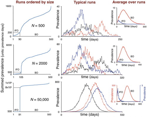
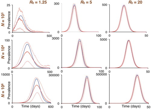
The effects of ensemble size n are fairly obvious: for example, compare the middle panel of individual runs and the left panel of averages depicted in Figure 5. To see the effects of N and ${\mathcal{R}}_0$ on the mean of ensembles of instantiations of the stochastic model, consider the $({\gamma }^{\mathrm{E}},k^{\mathrm{E}},{\gamma }^{\mathrm{I}},k^{\mathrm{I}})=(5,5,1,1)$ configuration of the model for the cases $\beta =0.25$ (${\mathcal{R}}_0=1.25$), $\beta =1$ (${\mathcal{R}}_0=5$), and $\beta =2$ (${\mathcal{R}}_0=20$), which correspond to, Runs 1, 17, and 33 in Table 1, for scenarios $N={10}^3$, ${10}^4$,and ${10}^6$. The results obtained are presented in Figure 6. From these results, we see that ensembles larger than n=100 are needed to smooth out the curves generated when ${\mathcal{R}}_0$ and N are both relatively small (e.g. ${\mathcal{R}}_0=1.25$ and $N={10}^3$; top left panel), but are quite smooth when either N is relatively large (e.g. ${\mathcal{R}}_0=1.25$ and $N={10}^6$; bottom left panel), or when ${\mathcal{R}}_0$ is somewhat larger (e.g. ${\mathcal{R}}_0=5$ and $N={10}^3$; top middle panel). When ${\mathcal{R}}_0=1.25$, the ensemble mean underestimates the deterministic solution (left column of panels) by 25–30%. This falls to just under 10% when ${\mathcal{R}}_0=5$ (centre column of panels), and below 2% when ${\mathcal{R}}_0=20$ (right column of panels).

Figure 6. The left, middle, and right columns are plots of prevalence obtained from the discrete deterministic model (blue curves) and averages over ensembles of 100 runs (n=100) of the discrete stochastic Erlang models (red curves; broken lines are ± one standard deviation around solid curve mean) for Cases 1, 17, and 33 (cf. Table 1).

Model comparisons

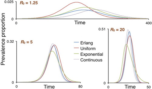
We compared the deterministic solutions obtained from the $(k^{\mathrm{E}},k^{\mathrm{I}},{\gamma }^{\mathrm{E}},{\gamma }^{\mathrm{I}})=(1,5,1,5)$ Erlang models (both discrete and continuous) with their ${\mathcal{R}}_0$-equivalent deterministic Uniform and Exponential discrete-time models for the scenarios ${\mathcal{R}}_0=1.25$ ($\beta =0.25$), ${\mathcal{R}}_0=5$ ($\beta =1$) and ${\mathcal{R}}_0=20$ ($\beta =0.4$). The prevalence curves obtained, normalized to proportions (since deterministic solutions do not depend on N) are presented in Figure 7. Except in cases with a low ${\mathcal{R}}_0$ value (top panel), the Uniform provides a much better fit to the Erlang model than the Exponential does.

Figure 7. The prevalence in the population (normalized to a proportion) is plotted for the continuous and discrete $(k^{\mathrm{E}},k^{\mathrm{I}},{\gamma }^{\mathrm{E}},{\gamma }^{\mathrm{I}})=(1,5,1,5)$ Erlang models (dotted and blue curves respectively), as well as their Uniform (brown curve) and Exponential (green curve) discrete-time counterparts for the cases $\beta =0.25$, 1 and 4 (${\mathcal{R}}_0=1.25$, 5, and 20 respectively).

Fitting models to Ebola data

Using published data from the Ebola outbreak in Liberia during the 74 weeks following initial reporting in March of 2014 (compiled by [5]), we fitted several of the proposed formulations to real outbreak data. The models tested on the Ebola data (the discrete and continuous Erlang) were compared to the discrete and continuous versions of the standard SEIR formulation (with an exponential distribution governing transitions between compartments) to judge the utility of the alternative methods for model fitting. Because the transmission rate was treated as a constant throughout the epidemic, only the initial quasi-exponential increase was used for the purposes of fitting. In order to fit these models to the subsequent decline in infections (when the population of susceptible hosts is not exhausted during the initial increase), assumptions regarding the form of the change in the transmission parameter (β) must be made. While some have used an exponential decay to represent this shifting β value over time [3], others have used threshold functions [34] or related the transmission parameter to environmental covariates like seasonality [43]. Fitting to the initial increase in the epidemic should be informative with regard to the ability of each alternative formulation to fit to real epidemic data without requiring a potentially confounding assumption about the form of the change in the transmission rate over time. As in [3], a total population size of ${10}^6$ was used for each model, and the epidemic was initialized with a single infected case.

The standard SEIR formulation, which consists of three parameters (β, γ, and σ), converged relatively quickly, as indicated by the resulting multivariate potential scale reduction factor (PSRF; a metric of MCMC convergence associated with Gelman and Rubin [19], where values close to 1 indicate success). The negative log-likelihood of the discrete model was lower than that of the continuous formulation, no matter the number of iterations, despite being slightly less computationally efficient. The MCMC sampling algorithm mixed well in both cases, with acceptance rates between approximately 0.1 and 0.6 generally treated as suitable (Table 3). Importantly, the ${\mathcal{R}}_0$ values for each of the models were fairly consistent with one another, ranging from 4.25 to 4.62 (Table 4).

Table 3. Diagnostic results of the standard SEIR Model using both discrete and continuous time formulations.

Model	Iterations (Burn-In)	Time (hrs)	Likelihood	Mixing Rate	Convergence
Discrete SEIR	50,000 (10,000)	0.831	−99.37	0.381	1.47
Discrete SEIR	100,000 (20,000)	1.651	−99.426	0.387	1.15
Discrete SEIR	200,000 (40,000)	3.265	−99.334	0.388	1.12
Continuous SEIR	50,000 (10,000)	0.403	−115.377	0.318	1.3
Continuous SEIR	100,000 (20,000)	0.812	−115.289	0.322	1.51
Continuous SEIR	200,000 (40,000)	1.577	−114.246	0.327	1.16

Note: The computational time required to run six parallel chains, the mixing rate (as determined by the mean acceptance rate across all chains) and convergence (PSRF), as well as the negative log-likelihood of the best fitting chain are displayed. Three different sets were run, each with a different number of iterations to illustrate how the diagnostic statistics and fit changed with additional time.

Table 4. The parameter values associated with the best fitting model (in terms of negative log-likelihood) are shown for each of the standard SEIR models.

Model	Iterations (Burn-In)	β	σ (days)	γ (days)	${\mathcal{R}}_0$
Discrete SEIR	50,000 (10,000)	0.181	22.421	25.415	4.596
Discrete SEIR	100,000 (20,000)	0.196	24.440	23.593	4.622
Discrete SEIR	200,000 (40,000)	0.198	24.621	23.248	4.605
Continuous SEIR	50,000 (10,000)	0.180	18.671	25.036	4.518
Continuous SEIR	100,000 (20,000)	0.192	20.337	23.976	4.594
Continuous SEIR	200,000 (40,000)	0.175	17.135	24.302	4.248

Note: Three of the parameters (σ, γ, and ${\mathcal{R}}_0$) were estimated directly using an MCMC approach, whereas β was derived based on the other parameter estimates.

The Erlang models have more dynamic model structures than the standard SEIR formulations due to the complications involved in altering the number of compartments through which exposed and infected individuals move. This resulted in substantially longer computation times for these models compared to the simpler SEIR models (Table 5). The Erlang formulations also required more iterations to converge consistently on the same parameter values. Despite nearly optimal mixing rates, the six chains of the discrete Erlang model still had PSRF values substantially higher than 1, indicating that even more iterations (and computational resources) were required for the six chains to converge on the same parameter estimates. The best fitting chains of the discrete Erlang model (after at least 100,000 iterations) did fit more closely to the data than the best fitting models from the discrete standard SEIR model (Table 5; Figure 8). This indicates that the discrete Erlang offers a more accurate representation of epidemic dynamics than the simple SEIR model, but the additional computation time and the failure to converge consistently on the same parameter values makes the method much more demanding than the approximation offered by the standard SEIR model. Notably, the ${\mathcal{R}}_0$ values estimated using the Erlang models ranged from 3.76 to 4.60, a slightly larger range than the standard SEIR models (likely due to the lack of convergence), but similar in magnitude to those obtained using the simpler alternatives (Table 6). In both cases, these ${\mathcal{R}}_0$ values are higher than previously published estimates for Ebola, which have ranged from 1.35 to 3.65 [28].

Figure 8. The incidence data from the first 155 days of the 2014 Ebola outbreak in Liberia are plotted together with output from the best fitting continuous and discrete SEIR and SE${}_n$I${}_m$R-Erlang models (corresponding to the fits that run for the longest number of iterations in each case), with details diagnostic fitting and parameter value details provided in Tables 3 and 6.

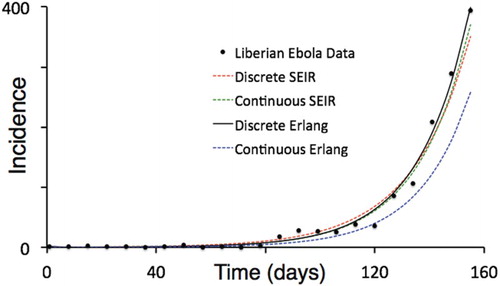
Table 5. Diagnostic results of the Erlang formulations using both discrete and continuous time formulations.

Model	Iterations (Burn-In)	Time (hrs)	Likelihood	Mixing rate	Convergence
Discrete Erlang	50,000 (10,000)	7.905	−108.36	0.231	6.12
Discrete Erlang	100,000 (20,000)	19.428	−98.522	0.244	4.03
Discrete Erlang	200,000 (40,000)	51.943	−92.633	0.275	5.24
Discrete Erlang	500,000 (100,000)	98.625	−92.424	0.232	4.96
Continuous Erlang	50,000 (10,000)	13.368	−120.624	0.193	5.77
Continuous Erlang	100,000 (20,000)	31.038	−118.533	0.235	5.62
Continuous Erlang	200,000 (40,000)	59.164	−118.258	0.218	2.00
Continuous Erlang	500,000 (200,000)*	106.123	−115.815	0.214	2.35

Note: The computational time required to run six parallel chains, the mixing rate (as determined by the mean acceptance rate across all chains) and convergence (PSRF), as well as the negative log-likelihood of the best fitting chain are displayed. Four different sets were run, each with a different number of iterations to illustrate how the diagnostic statistics and fit changed with additional time. The asterisk indicates the fact that final run of the continuous Erlang was analysed using a longer burn-in period of 200,000 iterations (40%) rather than the 20% used for the other runs.

Table 6. The parameter values associated with the best fitting model (in terms of negative log-likelihood) are shown for each of the Erlang models.

Model	Iterations (Burn-In)	β	$k^{\mathrm{E}}$	$k^{\mathrm{I}}$	${\gamma }^{\mathrm{E}}$	${\gamma }^{\mathrm{I}}$	${\mathcal{R}}_0$
Discrete Erlang	50,000 (10,000)	0.361	5	5	1.889	1.440	3.760
Discrete Erlang	100,000 (20,000)	0.316	5	5	1.468	1.172	4.044
Discrete Erlang	200,000 (40,000)	0.219	5	5	1.825	0.778	4.222
Discrete Erlang	500,000 (100,000)	0.203	5	5	1.887	0.708	4.301
Continuous Erlang	50,000 (10,000)	0.298	7	9	0.336	0.662	4.054
Continuous Erlang	100,000 (20,000)	0.323	7	8	0.307	0.562	4.598
Continuous Erlang	200,000 (40,000)	0.254	8	12	0.425	0.786	3.878
Continuous Erlang	500,000 (200,000)*	0.286	7	11	0.387	0.762	4.128

Note: In the discrete case, three of the parameters (β, ${\gamma }^{\mathrm{E}}$, and ${\gamma }^{\mathrm{I}}$), whereas the shape parameters ($k^{\mathrm{E}}$ and $k^{\mathrm{I}}$) were fixed at 5. These shape parameters were multiplied by 3 to determine the number of boxcars in the E and I classes to ensure that $\sim 99\mathrm{\%}$ of individuals made it through the E and I states. Finally, the ${\mathcal{R}}_0$ values were derived from the other parameter values. In the case of the continuous model, five parameters ($k^{\mathrm{E}}$, $k^{\mathrm{I}}$, ${\gamma }^{\mathrm{E}}$, ${\gamma }^{\mathrm{I}}$, and ${\mathcal{R}}_0$) were fit directly with the MCMC sampler, while β was derived from the other parameter estimates. The asterisk indicates the fact that final run of the continuous Erlang was analysed using a longer burn-in period of 200,000 iterations (40%) rather than the 20% used for the other runs.

The discrete stochastic Erlang model was not used to fit the empirical epidemic data because of the complexities involved in the interpretation of the results. Even when averages over a substantial number of instantiations are used to calculate the fit associated with a particular parameter set, the uncertainty bounds surrounding this mean may be just as important in producing the empirical data as the mean itself. A real-world epidemic is indeed a stochastic process, but it is unclear whether the epidemic represents an instantiation at one of the extremes around the set of parameters that govern the process or the mean or a realization somewhere in between. This fact hinders model fitting procedures in epidemiology when using a deterministic model as well. However, due to computational limitations, the most efficient method likely involves fitting a discrete deterministic model first, and then exploring the potential spread that an epidemic can exhibit around those resulting parameters using a stochastic formulation of the model.

Conclusion

Continuous-time Erlang SE${}_n$I${}_m$R models may be aesthetically appealing because epidemic events can arise at any time (i.e. time is continuous), and humped-shaped specific disease-class residence times provide better fits to real data than the exponentially distributed residence times associated with the standard single component SEIR model [49,56]. Data, however, are usually aggregated and binned into discrete-time intervals, not only for convenience, but also because the precise times of actual events (e.g. when exactly a particular individual was exposed to a dose of pathogen, or when exactly a particular individual became or ceased to be infectious) is not usually known. Thus, continuous models cannot be regarded as intrinsically more accurate than discrete models, particularly when noise within the data is taken into account. All else being equal, we should choose models that are computationally more tractable. This is particularly the case for discrete-time models where the interval is synchronized with the temporal aggregation of data, typically daily or weekly for fast epidemics, or monthly or quarterly for slow epidemics. Further, when extending formulations to incorporate stochasticity, discrete models are more easily implemented than having to apply a Gillespie or modified Gillespie algorithm to simulate continuous time stochastic processes, which may also require an unrealistic Poisson process assumption [17,18,54]. No matter how little or much stochasticity is associated with environmental factors, demographic stochasticity always plays a major role in epidemics because all epidemics start with a small number of infected individuals. This implies that even for values of ${\mathcal{R}}_0$ comfortably larger than 1 (e.g. in the range 2–4), the fadeout of an epidemic before it can breakout is an event we can expect to occasionally observe [2,10,24,45,47,48].

The real challenge in applying epidemic models is to either strategically identify key factors that lead to outbreaks (thereby providing a guide to reducing the risk of such outbreaks) or tactically manage ongoing epidemics through appropriate interventions. In both cases, we should avoid focusing our computational efforts on model fitting at the expense of numerical simulations to obtain broad comprehension: the imperative to find the best fitting set of parameters for the model at hand comes at the expense of obtaining a deeper understanding through exploratory simulations. This exploration includes a full assessment of possible ranges of outcomes due to stochastic factors (both demographic and environmental). Additional exploration requires that we incorporate factors that profoundly affect the course of epidemics, yet are not included in our SEIR formulations. Specifically, here we addressed the issue of replacing exponential residence times in disease classes with the more realistic distributed-delay residences times. We also overcome the issue of modelling declining transmission rates over time by fitting our models only to data from early stages of the epidemic.

Future studies that fit models to data that continue beyond the exponential outbreak phase need to include time-varying transmission rate functions of the form depicted in Equation (5(5) $\beta \left(t\right)=\frac{{\beta }_0}{1+{\left(\frac{t}{t_{\mathrm{c}}}\right)}^{\epsilon }},$(5) ). Equally important for many diseases is eliminating the assumption that the epidemic is occurring in a spatially homogeneous population. In these cases, models need to include spatial structure. This is most easily done by assuming a metapopulation structure: i.e. a small network of relatively large homogeneous subpopulations [6,30,36]. In the context of epidemics, spatial structure typically has two major components. The first is the way populations are distributed into major population centres, each of which can be assumed to constitute a homogeneous subpopulation. The second is to appropriately characterize the movement of individuals among subpopulations [32], particularly individuals who are infected, but still asymptomatic (e.g. individuals who are in class E, but make the transition to class I once they have moved).

Whatever approach is taken in future studies to modelling epidemics in populations with notable substructures – whether that substructure depends upon spatial organization, age, behavioural, or alternative means of categorizing individuals – computationally efficient stochastic models are needed. Further, these models should exhibit realistic residence-time properties for individuals within disease classes. The discrete time-to-go model formulated here represents a useful step towards satisfying the latter proposition.

Acknowledgments

WMG would like to thank Juliet Pulliam for hosting his visit in October 2016 to the South African Center for Epidemiological Modeling and Analysis (SACEMA) where his initial work on the SEIR time-to-go model began. WMG developed the discrete SEIR time-to-go formulation (Figure 1) and formulated the model equations reported in Section 2, as well as generating the comparative simulations (Figures 2–6). ERD fitted the models to the Liberian Ebola data and obtained the results reported in Tables 3-6. Both authors contributed to the writing and editing of the manuscript.

Disclosure statement

No potential conflict of interest was reported by the authors.

Additional information

Funding

This work in part was thus supported by South African Center for Epidemiological Modeling and Analysis and also by NIH Grant GM117617 to Jason Blackburn with WMG as subcontractor.

References

- M. Ajelli, B. Gonçalves, D. Balcan, V. Colizza, H. Hu, J.J. Ramasco, S. Merler, and A. Vespignani, Comparing large-scale computational approaches to epidemic modeling: Agent-based versus structured metapopulation models, BMC Infect. Dis. 10(1) (2010), p. 190. doi: 10.1186/1471-2334-10-190
- L.J. Allen, A primer on stochastic epidemic models: Formulation, numerical simulation, and analysis, Infect. Dis. Model. 2(2) (2017), pp. 128–142. doi: 10.1016/j.idm.2017.03.001
- C.L. Althaus, Estimating the reproduction number of Ebola Virus (EBOV) during the 2014 outbreak in West Africa, PLOS Curr. Outbreaks 6 (2014), doi:10.1371/currents.outbreaks.91afb5e0f279e7f29e7056095255b288.
- R.M. Anderson and R.M. May, Infectious Diseases of Humans: Dynamics and Control. Oxford: Oxford University Press, 1991.
- J.A. Backer and J. Wallinga, Spatiotemporal analysis of the 2014 Ebola epidemic in West Africa, PLOS Comput. Biol. 12(12) (2016), p. e1005210. doi: 10.1371/journal.pcbi.1005210
- D. Balcan, B. Gonçalves, H. Hu, J.J. Ramasco, V. Colizza, and A. Vespignani, Modeling the spatial spread of infectious diseases: The GLobal Epidemic and Mobility computational model, J. Comput. Sci. 1(3) (2010), pp. 132–145. doi: 10.1016/j.jocs.2010.07.002
- N. Bame, S. Bowong, J. Mbang, G. Sallet, and J.-J. Tewa, Global stability analysis for SEIS models with n latent classes, Math. Biosci. Eng. 5(1) (2008), pp. 20–33. doi: 10.3934/mbe.2008.5.20
- S. Blumberg and J.O. Lloyd-Smith, Inference of R0 and transmission heterogeneity from the size distribution of stuttering chains, PLoS Comput. Biol. 9(5) (2013), p. e1002993. doi: 10.1371/journal.pcbi.1002993
- S.P. Blythe and R.M. Anderson, Distributed incubation and infectious periods in models of the transmission dynamics of the human immunodeficiency virus (HIV), Math. Med. Biol. 5(1) (1988), pp. 1–19. doi: 10.1093/imammb/5.1.1
- T. Britton, Stochastic epidemic models: A survey, Math. Biosci. 225(1) (2010), pp. 24–35. doi: 10.1016/j.mbs.2010.01.006
- D.S. Burke, J.M. Epstein, D.A.T. Cummings, J.I. Parker, K.C. Cline, R.M. Singa, and S. Chakravarty, Individual-based computational modeling of smallpox epidemic control strategies, Acad. Emerg. Med. 13(11) (2006), pp. 1142–1149. doi: 10.1111/j.1553-2712.2006.tb01638.x
- A. Camacho, A.J. Kucharski, S. Funk, J. Breman, P. Piot, and W.J. Edmunds, Potential for large outbreaks of Ebola virus disease, Epidemics 9 (2014), pp. 70–78. doi: 10.1016/j.epidem.2014.09.003
- D. Clancy, SIR epidemic models with general infectious period distribution, Statist. Probab. Lett. 85 (2014), pp. 1–5. doi: 10.1016/j.spl.2013.10.017
- J.M. Cushing, Integrodifferential Equations and Delay Models in Population Dynamics, Vol. 20, Springer-Verlag, Berlin, 1977.
- O. Diekmann, J.A.P Heesterbeek, and J.A.J. Metz, On the definition and the computation of the basic reproduction ratio R0 in models for infectious diseases in heterogeneous populations, J. Math. Biol. 28(4) (1990), pp. 365–382. doi: 10.1007/BF00178324
- S. Funk, M. Salathé, and V.A. Jansen, Modelling the influence of human behaviour on the spread of infectious diseases: A review, J. R. Soc. Interface (2010), p. rsif20100142.
- D.T. Gillespie, A general method for numerically simulating the stochastic time evolution of coupled chemical reactions, J. Comput. Phys. 22(4) (1976), pp. 403–434. doi: 10.1016/0021-9991(76)90041-3
- D.T. Gillespie, Exact stochastic simulation of coupled chemical reactions, J. Phys. Chem. 81(25) (1977), pp. 2340–2361. doi: 10.1021/j100540a008
- A. Gelman and D.B. Rubin, Inference from iterative simulation using multiple sequences, Statist. Sci. 7 (1992), pp. 457–472. doi: 10.1214/ss/1177011136
- W.M. Getz, A hypothesis regarding the abruptness of density dependence and the growth rate of populations, Ecology 77(7) (1996), pp. 2014–2026. doi: 10.2307/2265697
- W.M. Getz and J.O. Lloyd-Smith, Basic methods for modeling the invasion and spread of contagious diseases, DIMACS Ser. Discrete Math. Theoret. Comput. Sci. 71 (2006), p. 87. doi: 10.1090/dimacs/071/05
- W.M. Getz and J. Pickering, Epidemic models: Thresholds and population regulation, Am. Nat. 121(6) (1983), pp. 892–898. doi: 10.1086/284112
- W.M. Getz, J.O. Lloyd-Smith, P.C. Cross, S. Bar-David, P.L. Johnson, and T.C. Porco, et al., Modeling the invasion and spread of contagious diseases in heterogeneous populations, in Disease Evolution: Models, Concepts, and Data Analyses, Vol. 71, Z. Feng, U. Dieckmann, and S.A. Levin, eds., American Mathematical Society, Providence, RI, 2006, pp. 113–144.
- W.M. Getz, J.-P . Gonzalez, R. Salter, J. Bangura, C. Carlson, M. Coomber, E. Dougherty, D. Kargbo, N.D. Wolfe and N. Wauquier, Tactics and strategies for managing Ebola outbreaks and the salience of immunization, Comput. Math. Methods Med. 2015 (2015), pp. 1–9. doi: 10.1155/2015/736507
- B. Grenfell, O. Bjørnstad, and J. Kappey, Travelling waves and spatial hierarchies in measles epidemics, Nature 414(6865) (2001), pp. 716–723. doi: 10.1038/414716a
- J.M. Heffernan, R.J. Smith, and L.M. Wahl, Perspectives on the basic reproductive ratio, J. R. Soc. Interf. 2(4) (2005), pp. 281–293. doi: 10.1098/rsif.2005.0042
- H.W. Hethcote, The mathematics of infectious diseases, SIAM Rev. 42(4) (2000), pp. 599–653. doi: 10.1137/S0036144500371907
- T. House, Epidemiological dynamics of Ebola outbreaks, Elife 3 (2014), p. e03908.
- H.S. Hurd, J.B. Kaneene, and J.W. Lloyd, A stochastic distributed-delay model of disease processes in dynamic populations, Prev. Vet. Med. 16(1) (1993), pp. 21–29. doi: 10.1016/0167-5877(93)90005-E
- M.J. Keeling, The effects of local spatial structure on epidemiological invasions, Proc. R. Soc. Lond. B 266(1421) (1999), pp. 859–867. doi: 10.1098/rspb.1999.0716
- A.A. King, M.D. de Cellès, F.M. Magpantay, and P. Rohani, Avoidable errors in the modelling of outbreaks of emerging pathogens, with special reference to Ebola, Proc. R. Soc. B 282 (2015), doi: 10.1098/rspb.2015.0347.
- A.M. Kramer, J.T. Pulliam, L.W. Alexander, A.W. Park, P. Rohani, and J.M. Drake, Spatial spread of the West Africa Ebola epidemic, Royal Soc. Open Sci. 3(8) (2016), doi: 10.1098/rsos.160294.
- M. Leclerc, T. Doré, C.A. Gilligan, P. Lucas, and J.A. Filipe, Estimating the delay between host infection and disease (incubation period) and assessing its significance to the epidemiology of plant diseases, PloS One 9(1) (2014), p. e86568. doi: 10.1371/journal.pone.0086568
- P.E. Lekone and B.F. Finkenstädt, Statistical inference in a stochastic epidemic SEIR model with control intervention: Ebola as a case study, Biometrics 62(4) (2006), pp. 1170–1177. doi: 10.1111/j.1541-0420.2006.00609.x
- A.L. Lloyd, Destabilization of epidemic models with the inclusion of realistic distributions of infectious periods, Proc. R. Soc. Lond. B 268(1470) (2001), pp. 985–993. doi: 10.1098/rspb.2001.1599
- A.L. Lloyd and V.A. Jansen, Spatiotemporal dynamics of epidemics: Synchrony in metapopulation models, Math. Biosci. 188(1) (2004), pp. 1–16. doi: 10.1016/j.mbs.2003.09.003
- J.O. Lloyd-Smith, A.P. Galvani, and W.M. Getz, Curtailing transmission of severe acute respiratory syndrome within a community and its hospital, Proc. R. Soc. Lond. B 270(1528) (2003), pp. 1979–1989. doi: 10.1098/rspb.2003.2481
- J.O. Lloyd-Smith, P.C. Cross, C.J. Briggs, M. Daugherty, W.M. Getz, J. Latto, M.S. Sanchez, A.B. Smith, and A. Swei, Should we expect population thresholds for wildlife disease?, Trends Ecol. Evol. 20(9) (2005), pp. 511–519. doi: 10.1016/j.tree.2005.07.004
- J.O. Lloyd-Smith, S. Funk, A.R. McLean, S. Riley, and J.L. Wood, Nine challenges in modelling the emergence of novel pathogens, Epidemics 10 (2015), pp. 35–39. doi: 10.1016/j.epidem.2014.09.002
- N. MacDonald, Time Lags in Biological Models, Springer-Verlag, Berlin, 1978.
- H. McCallum, N. Barlow, and J. Hone, How should pathogen transmission be modelled?, Trends Ecol. Evol. 16(6) (2001), pp. 295–300. doi: 10.1016/S0169-5347(01)02144-9
- B. Meerson and P.V. Sasorov, WKB theory of epidemic fade-out in stochastic populations, Phys. Rev. E 80(4) (2009), p. 041130. doi: 10.1103/PhysRevE.80.041130
- C.J.E. Metcalf, O.N. Bjørnstad, B.T. Grenfell, and V. Andreasen, Seasonality and comparative dynamics of six childhood infections in pre-vaccination Copenhagen, Proc. R. Soc. Lond. B 276(1676) (2009), pp. 4111–4118. doi: 10.1098/rspb.2009.1058
- J.A. Metz and O. Diekmann, The Dynamics of Physiologically Structured Populations, Vol. 68, Springer-Verlag, Berlin, 1986.
- I. Nåsell, The threshold concept in stochastic epidemic and endemic models, Epidemic models: their structure and relation to data 5 (1995), p. 71.
- I. Nåsell, On the time to extinction in recurrent epidemics, J. R. Stat. Soc. Ser. B Stat. Methodol. 61(2) (1999), pp. 309–330. doi: 10.1111/1467-9868.00178
- I. Nåsell, Stochastic models of some endemic infections, Math. Biosci. 179(1) (2002), pp. 1–19. doi: 10.1016/S0025-5564(02)00098-6
- I. Nåsell, A new look at the critical community size for childhood infections, Theor. Popul. Biol. 67(3) (2005), pp. 203–216. doi: 10.1016/j.tpb.2005.01.002
- P.D. O'Neill, Introduction and snapshot review: Relating infectious disease transmission models to data, Stat. Med. 29(20) (2010), pp. 2069–2077. doi: 10.1002/sim.3968
- I. Sazonov, M. Kelbert, and M.B. Gravenor, A two-stage model for the SIR outbreak: Accounting for the discrete and stochastic nature of the epidemic at the initial contamination stage, Math. Biosci. 234(2) (2011), pp. 108–117. doi: 10.1016/j.mbs.2011.09.002
- H. Smith, An Introduction to Delay Differential Equations with Applications to the Life Sciences, Vol. 57, Springer Science & Business Media, New York, 2010.
- D.L. Smith, K.E. Battle, S.I. Hay, C.M. Barker, T.W. Scott, and F.E. McKenzie, Ross, Macdonald, and a theory for the dynamics and control of mosquito-transmitted pathogens, PLoS Pathog. 8(4) (2012), p. e1002588. doi: 10.1371/journal.ppat.1002588
- P. Van den Driessche and J. Watmough, Reproduction numbers and sub-threshold endemic equilibria for compartmental models of disease transmission, Math. Biosci. 180(1) (2002), pp. 29–48. doi: 10.1016/S0025-5564(02)00108-6
- C.L. Vestergaard and M. Génois, Temporal Gillespie algorithm: Fast simulation of contagion processes on time-varying networks, PLoS Comput. Biol. 11(10) (2015), p. e1004579. doi: 10.1371/journal.pcbi.1004579
- J. Wallinga, P. Teunis, and M. Kretzschmar, Using data on social contacts to estimate age-specific transmission parameters for respiratory-spread infectious agents, Am. J. Epidemiol. 164(10) (2006), pp. 936–944. doi: 10.1093/aje/kwj317
- H.J. Wearing, P. Rohani, and M.J. Keeling, Appropriate models for the management of infectious diseases, PLoS Med. 2(7) (2005), p. e174. doi: 10.1371/journal.pmed.0020174