An age-structured within-host HIV-1 infection model with virus-to-cell and cell-to-cell transmissions

ABSTRACT

In this paper, a within-host HIV-1 infection model with virus-to-cell and direct cell-to-cell transmission and explicit age-since-infection structure for infected cells is investigated. It is shown that the model demonstrates a global threshold dynamics, fully described by the basic reproduction number. By analysing the corresponding characteristic equations, the local stability of an infection-free steady state and a chronic-infection steady state of the model is established. By using the persistence theory in infinite dimensional system, the uniform persistence of the system is established when the basic reproduction number is greater than unity. By means of suitable Lyapunov functionals and LaSalle's invariance principle, it is shown that if the basic reproduction number is less than unity, the infection-free steady state is globally asymptotically stable; if the basic reproduction number is greater than unity, the chronic-infection steady state is globally asymptotically stable. Numerical simulations are carried out to illustrate the feasibility of the theoretical results.

KEYWORDS:

• Within-host HIV-1 infection
• age since infection
• persistence
• Lyapunov functional
• LaSalle's invariance principle
• stability

2000 MATHEMATICS SUBJECT CLASSIFICATION:

• 37N25
• 92B05
• 37B25

1. Introduction

In past decades, great attention has been paid to the within-host dynamics of HIV using mathematical modelling. Mathematical modelling combined with experimental measurements has yielded important insights into HIV-1 pathogenesis and has enhanced progress in the understanding of HIV-1 infection (see, e.g. [1,6,16,18–21]). These models mainly investigated the dynamics of the target cells and infected cells, viral production and clearance, and the effects of antiretroviral drugs treatment. For decades it was believed that the spreading of HIV-1 within a host was mainly through free circulation of the viral particles with a repeated process. Models used to study HIV-1 infection have involved the concentrations of uninfected target cells, T, infected cells that are producing virus, $T^{\ast }$, and virus, V. The following classic and basic mathematical model describing HIV-1 infection dynamics was proposed and studied in [17,21]: (1) $\begin{array}{rl}\dot{T}\left(t\right)& =\lambda -dT\left(t\right)-\beta T\left(t\right)V\left(t\right),\\ {\dot{T}}^{\ast }\left(t\right)& =\beta T\left(t\right)V\left(t\right)-a{T}^{\ast }\left(t\right),\\ \dot{V}\left(t\right)& =k{T}^{\ast }\left(t\right)-uV\left(t\right),\end{array}$(1) where uninfected, susceptible cells are produced at a rate, λ, and die at rate dT, and become infected at rate $\beta TV$, where β is the rate constant describing the infection process; infected cells are produced at rate $\beta TV$ and die at rate $a{T}^{\ast }$; free virions are produced from infected cells at rate $k{T}^{\ast }$ and are removed at rate uV.

However, recent studies have revealed that a large number of viral particles can also be transferred from infected cells to uninfected cells through the formation of virally induced structures termed virological synapses (see, [2,4,8,25,26,29]). Cell-to-cell spread of HIV-1 between CD4${}^{+}$T cells is an efficient means of viral dissemination [25] and has been estimated to be several orders of magnitude more rapid than cell-free virus infection [2]. Cell-to-cell spread not only facilitates the rapid viral dissemination but may also promote immune invasion and, thereby, influence the disease [14]. It was shown in [27] that cell-to-cell spread of HIV-1 does reduce the efficacy of antiretroviral therapy, because cell-to-cell infection can cause multiple infections of target cells, which can in turn reduce the sensitivity to the antiretroviral drugs. The relative contribution of the two transmission pathways to virus growth through multiple rounds of replication has been examined by Sourisseau et al. [29], but it has not yet been quantified rigorously. In [10], by fitting a mathematical model to data reported in [29] as well as newly generated experimental data, Komarova et al. determined that free-virus and synaptic transmission make approximately equal contributions to virus growth in vitro.

In [11], Lai and Zou considered the following dynamical system model to incorporate both cell-to-cell infection mechanism and virus-to-cell infection mode: (2) $\begin{array}{rl}\dot{T}\left(t\right)& =\lambda -d_{T}T\left(t\right)-{\beta }_{1}T\left(t\right)V\left(t\right)-{\beta }_{2}T\left(t\right)T^{\ast }\left(t\right),\\ {\dot{T}}^{\ast }\left(t\right)& ={\beta }_1{\int }_0^{\mathrm{\infty }}f\left(s\right){\mathrm{e}}^{-\mu s}T(t-s)V(t-s)\mathrm{d}s\\ & +{\beta }_2{\int }_0^{\mathrm{\infty }}f\left(s\right){\mathrm{e}}^{-\mu s}T(t-s)T^{\ast }(t-s)\mathrm{d}s-\delta T^{\ast }\left(t\right),\\ \dot{V}\left(t\right)& =b{T}^{\ast }\left(t\right)-cV\left(t\right),\end{array}$(2) where $T\left(t\right),T^{\ast }\left(t\right)$ and $V\left(t\right)$ are concentrations of uninfected T cells, infected T cells, and free viral particles at time t, respectively. In system (2(2) $\begin{array}{rl}\dot{T}\left(t\right)& =\lambda -d_{T}T\left(t\right)-{\beta }_{1}T\left(t\right)V\left(t\right)-{\beta }_{2}T\left(t\right)T^{\ast }\left(t\right),\\ {\dot{T}}^{\ast }\left(t\right)& ={\beta }_1{\int }_0^{\mathrm{\infty }}f\left(s\right){\mathrm{e}}^{-\mu s}T(t-s)V(t-s)\mathrm{d}s\\ & +{\beta }_2{\int }_0^{\mathrm{\infty }}f\left(s\right){\mathrm{e}}^{-\mu s}T(t-s)T^{\ast }(t-s)\mathrm{d}s-\delta T^{\ast }\left(t\right),\\ \dot{V}\left(t\right)& =b{T}^{\ast }\left(t\right)-cV\left(t\right),\end{array}$(2) ), uninfected, susceptible cells are produced at a rate λ, and die at rate $d_{T}T\left(t\right)$, and become infected at rate ${\beta }_{1}TV+{\beta }_{2}T{T}^{\ast }$, where ${\beta }_1$ is the infection rate of free virus and ${\beta }_2$ is the infection rate of productively infected cells; infected cells are produced at rate ${\int }_0^{\mathrm{\infty }}f\left(s\right){\mathrm{e}}^{-\mu s}\left[{\beta }_{1}T\right(t-s\left)V\right(t-s)+{\beta }_{2}T(t-s\left)T^{\ast }\right(t-s\left)\right]\mathrm{d}s$ and die at rate $\delta T^{\ast }$. The time for infected cells to become productively infected may vary from individual to individual, and hence, a distribution function $f\left(s\right)$ is introduced to account for such variance. The term ${\mathrm{e}}^{-\mu s}$ accounts for the survival rates of cells that are infected at time t and become productively infected s time units later. Free virions are produced from infected cells at rate $b{T}^{\ast }$ and are removed at rate cV. In [12], Lai and Zou further studied an HIV-1 infection model with diffusion-limited cell-free virus transmission and cell-to-cell transfer and logistic target cell growth.

Note that in systems (1(1) $\begin{array}{rl}\dot{T}\left(t\right)& =\lambda -dT\left(t\right)-\beta T\left(t\right)V\left(t\right),\\ {\dot{T}}^{\ast }\left(t\right)& =\beta T\left(t\right)V\left(t\right)-a{T}^{\ast }\left(t\right),\\ \dot{V}\left(t\right)& =k{T}^{\ast }\left(t\right)-uV\left(t\right),\end{array}$(1) ) and (2(2) $\begin{array}{rl}\dot{T}\left(t\right)& =\lambda -d_{T}T\left(t\right)-{\beta }_{1}T\left(t\right)V\left(t\right)-{\beta }_{2}T\left(t\right)T^{\ast }\left(t\right),\\ {\dot{T}}^{\ast }\left(t\right)& ={\beta }_1{\int }_0^{\mathrm{\infty }}f\left(s\right){\mathrm{e}}^{-\mu s}T(t-s)V(t-s)\mathrm{d}s\\ & +{\beta }_2{\int }_0^{\mathrm{\infty }}f\left(s\right){\mathrm{e}}^{-\mu s}T(t-s)T^{\ast }(t-s)\mathrm{d}s-\delta T^{\ast }\left(t\right),\\ \dot{V}\left(t\right)& =b{T}^{\ast }\left(t\right)-cV\left(t\right),\end{array}$(2) ), both the death rate and virus production rate of infected cells are assumed to be constant. It was reported in [23] that virus production increases exponentially with the age of the infected cell in the case of simian immunodeficiency virus-infected CD4${}^{+}$ T cells in rhesus macaques. Recently, age-structured within-host HIV infection models have received increasing interest due to their greater flexibility in modelling variations in the death rate of productively infected T cells and the production rate of viral particles as a function of the length of time a T cell has been infected [15]. In [15], Nelson et al. developed the following age-structured within-host HIV-1 infection model: (3) $\begin{array}{rl}& \dot{T}\left(t\right)=s-d_{T}T\left(t\right)-\beta T\left(t\right)V\left(t\right),\\ & \frac{\mathrm{\partial }{T}^{\ast }(a,t)}{\mathrm{\partial }t}+\frac{\mathrm{\partial }{T}^{\ast }(a,t)}{\mathrm{\partial }a}=-\mu \left(a\right)T^{\ast }(a,t),\\ & \dot{V}\left(t\right)={\int }_0^{\mathrm{\infty }}p\left(a\right)T^{\ast }(a,t)\mathrm{d}a-uV\left(t\right),\end{array}$(3) with boundary condition $T^{\ast }(0,t)=\beta T\left(t\right)V\left(t\right)$. In system (3(3) $\begin{array}{rl}& \dot{T}\left(t\right)=s-d_{T}T\left(t\right)-\beta T\left(t\right)V\left(t\right),\\ & \frac{\mathrm{\partial }{T}^{\ast }(a,t)}{\mathrm{\partial }t}+\frac{\mathrm{\partial }{T}^{\ast }(a,t)}{\mathrm{\partial }a}=-\mu \left(a\right)T^{\ast }(a,t),\\ & \dot{V}\left(t\right)={\int }_0^{\mathrm{\infty }}p\left(a\right)T^{\ast }(a,t)\mathrm{d}a-uV\left(t\right),\end{array}$(3) ), $T^{\ast }(a,t)$ denotes the density of infected T cells of infection age a (i.e. the time that has elapsed since an HIV virion has penetrated the cell) at time t, $\mu \left(a\right)$ is the age-dependent per capita death rate of infected cells, $p\left(a\right)$ is the viral production rate of an infected cell with age a. The age of cellular infection plays a key role in determining the rate of viral particle production per productively infected T cell and how long the productively infected T cell lives. In [24], in order to assess the effect of different combination therapies on viral dynamics, Rong et al. incorporated treatment with three different classes of drugs into the age-structured model. In [7], by using the direct Lyapunov method, Huang et al. established the global stability of feasible steady states of system (3(3) $\begin{array}{rl}& \dot{T}\left(t\right)=s-d_{T}T\left(t\right)-\beta T\left(t\right)V\left(t\right),\\ & \frac{\mathrm{\partial }{T}^{\ast }(a,t)}{\mathrm{\partial }t}+\frac{\mathrm{\partial }{T}^{\ast }(a,t)}{\mathrm{\partial }a}=-\mu \left(a\right)T^{\ast }(a,t),\\ & \dot{V}\left(t\right)={\int }_0^{\mathrm{\infty }}p\left(a\right)T^{\ast }(a,t)\mathrm{d}a-uV\left(t\right),\end{array}$(3) ).

We note that the infection process in system (3(3) $\begin{array}{rl}& \dot{T}\left(t\right)=s-d_{T}T\left(t\right)-\beta T\left(t\right)V\left(t\right),\\ & \frac{\mathrm{\partial }{T}^{\ast }(a,t)}{\mathrm{\partial }t}+\frac{\mathrm{\partial }{T}^{\ast }(a,t)}{\mathrm{\partial }a}=-\mu \left(a\right)T^{\ast }(a,t),\\ & \dot{V}\left(t\right)={\int }_0^{\mathrm{\infty }}p\left(a\right)T^{\ast }(a,t)\mathrm{d}a-uV\left(t\right),\end{array}$(3) ) is assumed to be governed by the mass-action principle, that is, the infection rate per host and per virus is a constant. However, experiments reported in [3] strongly suggested that the infection rate of microparasitic infections is an increasing function of the parasite dose, and is usually sigmoidal in shape. In [22], to place the model on more sound biological grounds, Regoes et al. replaced the mass-action infection rate with a dose-dependent infection rate.

Motivated by the works of Lai and Zou [11], Nelson et al. [15] and Regoes et al. [22], in the present paper, we are concerned with the joint effects of age since infection, direct cell-to-cell transfer and virus-to-cell infection on the dynamics of HIV-1 infection. To this end, we consider the following within-host HIV-1 infection model: (4) $\begin{array}{rl}& \dot{x}\left(t\right)=s-\mathrm{d}x\left(t\right)-\frac{\beta x\left(t\right)v\left(t\right)}{1+\alpha v\left(t\right)}-x\left(t\right){\int }_0^{\mathrm{\infty }}{\beta }_1\left(a\right)y(a,t)\mathrm{d}a,\\ & \frac{\mathrm{\partial }y(a,t)}{\mathrm{\partial }t}+\frac{\mathrm{\partial }y(a,t)}{\mathrm{\partial }a}=-\mu \left(a\right)y(a,t),\\ & \dot{v}\left(t\right)={\int }_0^{\mathrm{\infty }}k\left(a\right)y(a,t)\mathrm{d}a-uv\left(t\right),\end{array}$(4) with boundary condition (5) $y(0,t)=\frac{\beta x\left(t\right)v\left(t\right)}{1+\alpha v\left(t\right)}+x\left(t\right){\int }_0^{\mathrm{\infty }}{\beta }_1\left(a\right)y(a,t)\mathrm{d}a,t>0,$(5) and initial condition (6) $X_0:=\left(x\right(0),y(\cdot ,0),v(0\left)\right)=(x^0,y_0(\cdot ),v^0)\in \mathcal{X},$(6) where $\mathcal{X}={\mathbb{R}}^{+}\times L_{+}^1(0,\mathrm{\infty })\times {\mathbb{R}}^{+}$, $L_{+}^1(0,\mathrm{\infty })$ is the set of all integrable functions from $(0,\mathrm{\infty })$ into ${\mathbb{R}}^{+}=[0,\mathrm{\infty })$.

In system (4(4) $\begin{array}{rl}& \dot{x}\left(t\right)=s-\mathrm{d}x\left(t\right)-\frac{\beta x\left(t\right)v\left(t\right)}{1+\alpha v\left(t\right)}-x\left(t\right){\int }_0^{\mathrm{\infty }}{\beta }_1\left(a\right)y(a,t)\mathrm{d}a,\\ & \frac{\mathrm{\partial }y(a,t)}{\mathrm{\partial }t}+\frac{\mathrm{\partial }y(a,t)}{\mathrm{\partial }a}=-\mu \left(a\right)y(a,t),\\ & \dot{v}\left(t\right)={\int }_0^{\mathrm{\infty }}k\left(a\right)y(a,t)\mathrm{d}a-uv\left(t\right),\end{array}$(4) ), $x\left(t\right)$ represents the concentration of uninfected target T cells at time t, $y(a,t)$ denotes the density of infected T cells of infection age a (i.e. the time that has elapsed since an HIV virion has penetrated cell) at time t, and $v\left(t\right)$ denotes the concentration of infectious free virion at time t. The definitions of all parameters in system (4(4) $\begin{array}{rl}& \dot{x}\left(t\right)=s-\mathrm{d}x\left(t\right)-\frac{\beta x\left(t\right)v\left(t\right)}{1+\alpha v\left(t\right)}-x\left(t\right){\int }_0^{\mathrm{\infty }}{\beta }_1\left(a\right)y(a,t)\mathrm{d}a,\\ & \frac{\mathrm{\partial }y(a,t)}{\mathrm{\partial }t}+\frac{\mathrm{\partial }y(a,t)}{\mathrm{\partial }a}=-\mu \left(a\right)y(a,t),\\ & \dot{v}\left(t\right)={\int }_0^{\mathrm{\infty }}k\left(a\right)y(a,t)\mathrm{d}a-uv\left(t\right),\end{array}$(4) ) are listed in Table 1.

Table 1. The definitions of the parameters in system (4(4) $\begin{array}{rl}& \dot{x}\left(t\right)=s-\mathrm{d}x\left(t\right)-\frac{\beta x\left(t\right)v\left(t\right)}{1+\alpha v\left(t\right)}-x\left(t\right){\int }_0^{\mathrm{\infty }}{\beta }_1\left(a\right)y(a,t)\mathrm{d}a,\\ & \frac{\mathrm{\partial }y(a,t)}{\mathrm{\partial }t}+\frac{\mathrm{\partial }y(a,t)}{\mathrm{\partial }a}=-\mu \left(a\right)y(a,t),\\ & \dot{v}\left(t\right)={\int }_0^{\mathrm{\infty }}k\left(a\right)y(a,t)\mathrm{d}a-uv\left(t\right),\end{array}$(4) ).

Parameters	Description
s	The recruitment rate of healthy T cells
d	The per capita death rate of uninfected cells
u	Clearance rate of virions
α	Saturation constant
β	The rate at which an uninfected cell becomes infected by an infectious virus
a	Age of infection, that is, the time since an HIV virion penetrated cell
${\beta }_1\left(a\right)$	The infection rate of productively infected cells with age a
$\mu \left(a\right)$	The age-dependent per capita death rate of infected cells
$k\left(a\right)$	The viral production rate of an infected cell with age a

We make the following assumptions on the parameters in system (4(4) $\begin{array}{rl}& \dot{x}\left(t\right)=s-\mathrm{d}x\left(t\right)-\frac{\beta x\left(t\right)v\left(t\right)}{1+\alpha v\left(t\right)}-x\left(t\right){\int }_0^{\mathrm{\infty }}{\beta }_1\left(a\right)y(a,t)\mathrm{d}a,\\ & \frac{\mathrm{\partial }y(a,t)}{\mathrm{\partial }t}+\frac{\mathrm{\partial }y(a,t)}{\mathrm{\partial }a}=-\mu \left(a\right)y(a,t),\\ & \dot{v}\left(t\right)={\int }_0^{\mathrm{\infty }}k\left(a\right)y(a,t)\mathrm{d}a-uv\left(t\right),\end{array}$(4) ).

(H1)	$k,\mu ,{\beta }_1\in L_{+}^1(0,\mathrm{\infty })$, let $\overline{k},\overline{\mu },{\overline{\beta }}_1$ be the essential supremums of $k,\mu ,{\beta }_1$, respectively;
(H2)	${\beta }_1\left(a\right)$ is Lipschitz continuous on ${\mathbb{R}}^{+}$ with Lipschitz coefficient $M_{{\beta }_1}$;
(H3)	There is a positive constant ${\mu }_0\le min\{d,u\}$ such that $\mu \left(a\right)\ge {\mu }_0$ for all $a\ge 0$.

Using the theory of age-structured dynamical systems developed in [9,30], we can verify that system (4(4) $\begin{array}{rl}& \dot{x}\left(t\right)=s-\mathrm{d}x\left(t\right)-\frac{\beta x\left(t\right)v\left(t\right)}{1+\alpha v\left(t\right)}-x\left(t\right){\int }_0^{\mathrm{\infty }}{\beta }_1\left(a\right)y(a,t)\mathrm{d}a,\\ & \frac{\mathrm{\partial }y(a,t)}{\mathrm{\partial }t}+\frac{\mathrm{\partial }y(a,t)}{\mathrm{\partial }a}=-\mu \left(a\right)y(a,t),\\ & \dot{v}\left(t\right)={\int }_0^{\mathrm{\infty }}k\left(a\right)y(a,t)\mathrm{d}a-uv\left(t\right),\end{array}$(4) ) has a unique solution $\left(x\right(t),y(\cdot ,t),v(t\left)\right)$ satisfying the boundary condition (5(5) $y(0,t)=\frac{\beta x\left(t\right)v\left(t\right)}{1+\alpha v\left(t\right)}+x\left(t\right){\int }_0^{\mathrm{\infty }}{\beta }_1\left(a\right)y(a,t)\mathrm{d}a,t>0,$(5) ) and the initial condition (6(6) $X_0:=\left(x\right(0),y(\cdot ,0),v(0\left)\right)=(x^0,y_0(\cdot ),v^0)\in \mathcal{X},$(6) ). Moreover, it is easy to show that all solutions of system (4(4) $\begin{array}{rl}& \dot{x}\left(t\right)=s-\mathrm{d}x\left(t\right)-\frac{\beta x\left(t\right)v\left(t\right)}{1+\alpha v\left(t\right)}-x\left(t\right){\int }_0^{\mathrm{\infty }}{\beta }_1\left(a\right)y(a,t)\mathrm{d}a,\\ & \frac{\mathrm{\partial }y(a,t)}{\mathrm{\partial }t}+\frac{\mathrm{\partial }y(a,t)}{\mathrm{\partial }a}=-\mu \left(a\right)y(a,t),\\ & \dot{v}\left(t\right)={\int }_0^{\mathrm{\infty }}k\left(a\right)y(a,t)\mathrm{d}a-uv\left(t\right),\end{array}$(4) ) with the boundary condition (5(5) $y(0,t)=\frac{\beta x\left(t\right)v\left(t\right)}{1+\alpha v\left(t\right)}+x\left(t\right){\int }_0^{\mathrm{\infty }}{\beta }_1\left(a\right)y(a,t)\mathrm{d}a,t>0,$(5) ) and the initial condition (6(6) $X_0:=\left(x\right(0),y(\cdot ,0),v(0\left)\right)=(x^0,y_0(\cdot ),v^0)\in \mathcal{X},$(6) ) are defined on $[0,+\mathrm{\infty })$ and remain positive for all $t\ge 0$. Furthermore, $\mathcal{X}$ is positively invariant and system (4(4) $\begin{array}{rl}& \dot{x}\left(t\right)=s-\mathrm{d}x\left(t\right)-\frac{\beta x\left(t\right)v\left(t\right)}{1+\alpha v\left(t\right)}-x\left(t\right){\int }_0^{\mathrm{\infty }}{\beta }_1\left(a\right)y(a,t)\mathrm{d}a,\\ & \frac{\mathrm{\partial }y(a,t)}{\mathrm{\partial }t}+\frac{\mathrm{\partial }y(a,t)}{\mathrm{\partial }a}=-\mu \left(a\right)y(a,t),\\ & \dot{v}\left(t\right)={\int }_0^{\mathrm{\infty }}k\left(a\right)y(a,t)\mathrm{d}a-uv\left(t\right),\end{array}$(4) ) exhibits a continuous semi-flow $\mathrm{\Phi }:{\mathbb{R}}^{+}\times \mathcal{X}\to \mathcal{X}$, namely, ${\mathrm{\Phi }}_t\left(X_0\right)=\mathrm{\Phi }(t,X_0):=\left(x\right(t),y(\cdot ,t),v(t\left)\right),t\ge 0,X_0\in \mathcal{X}.$ Given a point $(x,\varphi ,z)\in \mathcal{X}$, one has the norm $\Vert (x,\varphi ,z){\Vert }_{\mathcal{X}}:=x+{\int }_0^{\mathrm{\infty }}\varphi \left(a\right)\mathrm{d}a+z$.

In this paper, our primary goal is to carry out a complete mathematical analysis of system (4(4) $\begin{array}{rl}& \dot{x}\left(t\right)=s-\mathrm{d}x\left(t\right)-\frac{\beta x\left(t\right)v\left(t\right)}{1+\alpha v\left(t\right)}-x\left(t\right){\int }_0^{\mathrm{\infty }}{\beta }_1\left(a\right)y(a,t)\mathrm{d}a,\\ & \frac{\mathrm{\partial }y(a,t)}{\mathrm{\partial }t}+\frac{\mathrm{\partial }y(a,t)}{\mathrm{\partial }a}=-\mu \left(a\right)y(a,t),\\ & \dot{v}\left(t\right)={\int }_0^{\mathrm{\infty }}k\left(a\right)y(a,t)\mathrm{d}a-uv\left(t\right),\end{array}$(4) ) with the boundary condition (5(5) $y(0,t)=\frac{\beta x\left(t\right)v\left(t\right)}{1+\alpha v\left(t\right)}+x\left(t\right){\int }_0^{\mathrm{\infty }}{\beta }_1\left(a\right)y(a,t)\mathrm{d}a,t>0,$(5) ) and the initial condition (6(6) $X_0:=\left(x\right(0),y(\cdot ,0),v(0\left)\right)=(x^0,y_0(\cdot ),v^0)\in \mathcal{X},$(6) ) and establish its global dynamics. The organization of this paper is as follows. In the next section, we are concerned with the asymptotic smoothness of the semi-flow generated by system (4(4) $\begin{array}{rl}& \dot{x}\left(t\right)=s-\mathrm{d}x\left(t\right)-\frac{\beta x\left(t\right)v\left(t\right)}{1+\alpha v\left(t\right)}-x\left(t\right){\int }_0^{\mathrm{\infty }}{\beta }_1\left(a\right)y(a,t)\mathrm{d}a,\\ & \frac{\mathrm{\partial }y(a,t)}{\mathrm{\partial }t}+\frac{\mathrm{\partial }y(a,t)}{\mathrm{\partial }a}=-\mu \left(a\right)y(a,t),\\ & \dot{v}\left(t\right)={\int }_0^{\mathrm{\infty }}k\left(a\right)y(a,t)\mathrm{d}a-uv\left(t\right),\end{array}$(4) ). In Section 3, we calculate the basic reproduction number and investigate the existence of feasible steady states of system (4(4) $\begin{array}{rl}& \dot{x}\left(t\right)=s-\mathrm{d}x\left(t\right)-\frac{\beta x\left(t\right)v\left(t\right)}{1+\alpha v\left(t\right)}-x\left(t\right){\int }_0^{\mathrm{\infty }}{\beta }_1\left(a\right)y(a,t)\mathrm{d}a,\\ & \frac{\mathrm{\partial }y(a,t)}{\mathrm{\partial }t}+\frac{\mathrm{\partial }y(a,t)}{\mathrm{\partial }a}=-\mu \left(a\right)y(a,t),\\ & \dot{v}\left(t\right)={\int }_0^{\mathrm{\infty }}k\left(a\right)y(a,t)\mathrm{d}a-uv\left(t\right),\end{array}$(4) ). In Section 4, by analysing corresponding characteristic equations, we study the local asymptotic stability of an infection-free steady state and a chronic-infection steady state of system (4(4) $\begin{array}{rl}& \dot{x}\left(t\right)=s-\mathrm{d}x\left(t\right)-\frac{\beta x\left(t\right)v\left(t\right)}{1+\alpha v\left(t\right)}-x\left(t\right){\int }_0^{\mathrm{\infty }}{\beta }_1\left(a\right)y(a,t)\mathrm{d}a,\\ & \frac{\mathrm{\partial }y(a,t)}{\mathrm{\partial }t}+\frac{\mathrm{\partial }y(a,t)}{\mathrm{\partial }a}=-\mu \left(a\right)y(a,t),\\ & \dot{v}\left(t\right)={\int }_0^{\mathrm{\infty }}k\left(a\right)y(a,t)\mathrm{d}a-uv\left(t\right),\end{array}$(4) ). In Section 5, using the persistence theory in infinite dimensional system developed by Hale and Waltman in [5], the uniform persistence of the semi-flow generated by system (4(4) $\begin{array}{rl}& \dot{x}\left(t\right)=s-\mathrm{d}x\left(t\right)-\frac{\beta x\left(t\right)v\left(t\right)}{1+\alpha v\left(t\right)}-x\left(t\right){\int }_0^{\mathrm{\infty }}{\beta }_1\left(a\right)y(a,t)\mathrm{d}a,\\ & \frac{\mathrm{\partial }y(a,t)}{\mathrm{\partial }t}+\frac{\mathrm{\partial }y(a,t)}{\mathrm{\partial }a}=-\mu \left(a\right)y(a,t),\\ & \dot{v}\left(t\right)={\int }_0^{\mathrm{\infty }}k\left(a\right)y(a,t)\mathrm{d}a-uv\left(t\right),\end{array}$(4) ) is established when the basic reproduction number is greater than unity. In Section 6, we are concerned with the global stability of each of feasible steady states by constructing suitable Lyapunov functionals and using LaSalle's invariance principle. In Section 7, numerical examples are carried out to illustrate the feasibility of theoretical results. A brief discussion is given in Section 8 to conclude this work.

2. Asymptotic smoothness

In order to study the global dynamics of system (4(4) $\begin{array}{rl}& \dot{x}\left(t\right)=s-\mathrm{d}x\left(t\right)-\frac{\beta x\left(t\right)v\left(t\right)}{1+\alpha v\left(t\right)}-x\left(t\right){\int }_0^{\mathrm{\infty }}{\beta }_1\left(a\right)y(a,t)\mathrm{d}a,\\ & \frac{\mathrm{\partial }y(a,t)}{\mathrm{\partial }t}+\frac{\mathrm{\partial }y(a,t)}{\mathrm{\partial }a}=-\mu \left(a\right)y(a,t),\\ & \dot{v}\left(t\right)={\int }_0^{\mathrm{\infty }}k\left(a\right)y(a,t)\mathrm{d}a-uv\left(t\right),\end{array}$(4) ), in this section, we need to verify the asymptotic smoothness of the semi-flow $\left\{\mathrm{\Phi }\right(t){\}}_{t\ge 0}$ generated by system (4(4) $\begin{array}{rl}& \dot{x}\left(t\right)=s-\mathrm{d}x\left(t\right)-\frac{\beta x\left(t\right)v\left(t\right)}{1+\alpha v\left(t\right)}-x\left(t\right){\int }_0^{\mathrm{\infty }}{\beta }_1\left(a\right)y(a,t)\mathrm{d}a,\\ & \frac{\mathrm{\partial }y(a,t)}{\mathrm{\partial }t}+\frac{\mathrm{\partial }y(a,t)}{\mathrm{\partial }a}=-\mu \left(a\right)y(a,t),\\ & \dot{v}\left(t\right)={\int }_0^{\mathrm{\infty }}k\left(a\right)y(a,t)\mathrm{d}a-uv\left(t\right),\end{array}$(4) ).

2.1. Boundedness of solutions

Denote (7) $\pi \left(a\right)={\mathrm{e}}^{-{\int }_0^a\mu \left(s\right)\mathrm{d}s}\mathrm{for}a\in {\mathbb{R}}^{+}.$(7) It follows from (H1) and (H3) that $0<{\mathrm{e}}^{-\overline{\mu }a}\le \pi \left(a\right)\le {\mathrm{e}}^{-{\mu }_{0}a}$ for all $a\ge 0$. Clearly, $\pi \left(a\right)$ is a deceasing function.

Let ${\mathrm{\Phi }}_t\left(X_0\right)=\mathrm{\Phi }(t,X_0):=\left(x\right(t),y(a,t),v(t\left)\right)$ be any non-negative solution of system (4(4) $\begin{array}{rl}& \dot{x}\left(t\right)=s-\mathrm{d}x\left(t\right)-\frac{\beta x\left(t\right)v\left(t\right)}{1+\alpha v\left(t\right)}-x\left(t\right){\int }_0^{\mathrm{\infty }}{\beta }_1\left(a\right)y(a,t)\mathrm{d}a,\\ & \frac{\mathrm{\partial }y(a,t)}{\mathrm{\partial }t}+\frac{\mathrm{\partial }y(a,t)}{\mathrm{\partial }a}=-\mu \left(a\right)y(a,t),\\ & \dot{v}\left(t\right)={\int }_0^{\mathrm{\infty }}k\left(a\right)y(a,t)\mathrm{d}a-uv\left(t\right),\end{array}$(4) ) with the boundary condition (5(5) $y(0,t)=\frac{\beta x\left(t\right)v\left(t\right)}{1+\alpha v\left(t\right)}+x\left(t\right){\int }_0^{\mathrm{\infty }}{\beta }_1\left(a\right)y(a,t)\mathrm{d}a,t>0,$(5) ) and the initial condition (6(6) $X_0:=\left(x\right(0),y(\cdot ,0),v(0\left)\right)=(x^0,y_0(\cdot ),v^0)\in \mathcal{X},$(6) ). Integrating the second equation of system (4(4) $\begin{array}{rl}& \dot{x}\left(t\right)=s-\mathrm{d}x\left(t\right)-\frac{\beta x\left(t\right)v\left(t\right)}{1+\alpha v\left(t\right)}-x\left(t\right){\int }_0^{\mathrm{\infty }}{\beta }_1\left(a\right)y(a,t)\mathrm{d}a,\\ & \frac{\mathrm{\partial }y(a,t)}{\mathrm{\partial }t}+\frac{\mathrm{\partial }y(a,t)}{\mathrm{\partial }a}=-\mu \left(a\right)y(a,t),\\ & \dot{v}\left(t\right)={\int }_0^{\mathrm{\infty }}k\left(a\right)y(a,t)\mathrm{d}a-uv\left(t\right),\end{array}$(4) ) along the characteristic line $t-a=\mathrm{const}$. yields (8) $y(a,t)=\{\begin{array}{ll}L(t-a)\pi \left(a\right),& 0\le a<t,\\ y_0(a-t)\frac{\pi \left(a\right)}{\pi (a-t)},& 0\le t\le a,\end{array}$(8) where $L\left(t\right):=y(0,t)=\beta x\left(t\right)v\left(t\right)/(1+\alpha v(t\left)\right)+x\left(t\right){\int }_0^{\mathrm{\infty }}{\beta }_1\left(a\right)y(a,t)\mathrm{d}a$.

Denote $\Vert X_0{\Vert }_{\mathcal{X}}=x^0+{\int }_0^{\mathrm{\infty }}{y}_0\left(a\right)\mathrm{d}a+v^0$ and $N\left(t\right)=\Vert \mathrm{\Phi }(t,X_0){\Vert }_{\mathcal{X}}=x\left(t\right)+{\int }_0^{\mathrm{\infty }}y(a,t)\mathrm{d}a+v\left(t\right)$.

Proposition 2.1

For system (4(4) $\begin{array}{rl}& \dot{x}\left(t\right)=s-\mathrm{d}x\left(t\right)-\frac{\beta x\left(t\right)v\left(t\right)}{1+\alpha v\left(t\right)}-x\left(t\right){\int }_0^{\mathrm{\infty }}{\beta }_1\left(a\right)y(a,t)\mathrm{d}a,\\ & \frac{\mathrm{\partial }y(a,t)}{\mathrm{\partial }t}+\frac{\mathrm{\partial }y(a,t)}{\mathrm{\partial }a}=-\mu \left(a\right)y(a,t),\\ & \dot{v}\left(t\right)={\int }_0^{\mathrm{\infty }}k\left(a\right)y(a,t)\mathrm{d}a-uv\left(t\right),\end{array}$(4) ), the following statements hold.

1. $\left(\mathrm{d}/\mathrm{d}t\right)N\left(t\right)\le s+\overline{k}max\{s/{\mu }_0,\Vert X_0{\Vert }_{\mathcal{X}}\}-{\mu }_{0}N\left(t\right)$ for all $t\ge 0;$

2. $N\left(t\right)\le max\{s/{\mu }_0+(\overline{k}/{\mu }_0)max\{s/{\mu }_0,\Vert X_0{\Vert }_{\mathcal{X}}\},\Vert X_0{\Vert }_{\mathcal{X}}\}$ for all $t\ge 0;$

3. $\underset{t\to +\mathrm{\infty }}{lim sup}N\left(t\right)\le s(1+\overline{k}/{\mu }_0)/{\mu }_0;$

4. ${\mathrm{\Phi }}_t$ is point dissipative: there is a bounded set that attracts all points in $\mathcal{X}$.

Proof.

It follows from Equations (4(4) $\begin{array}{rl}& \dot{x}\left(t\right)=s-\mathrm{d}x\left(t\right)-\frac{\beta x\left(t\right)v\left(t\right)}{1+\alpha v\left(t\right)}-x\left(t\right){\int }_0^{\mathrm{\infty }}{\beta }_1\left(a\right)y(a,t)\mathrm{d}a,\\ & \frac{\mathrm{\partial }y(a,t)}{\mathrm{\partial }t}+\frac{\mathrm{\partial }y(a,t)}{\mathrm{\partial }a}=-\mu \left(a\right)y(a,t),\\ & \dot{v}\left(t\right)={\int }_0^{\mathrm{\infty }}k\left(a\right)y(a,t)\mathrm{d}a-uv\left(t\right),\end{array}$(4) )–(6(6) $X_0:=\left(x\right(0),y(\cdot ,0),v(0\left)\right)=(x^0,y_0(\cdot ),v^0)\in \mathcal{X},$(6) ) that (9) $\begin{array}{rl}\frac{\mathrm{d}}{\mathrm{d}t}\left(x\right(t)+{\int }_0^{\mathrm{\infty }}y(a,t\left)\mathrm{d}a\right)& =s-\mathrm{d}x\left(t\right)-\frac{\beta x\left(t\right)v\left(t\right)}{1+\alpha v\left(t\right)}-x\left(t\right){\int }_0^{\mathrm{\infty }}{\beta }_1\left(a\right)y(a,t)\mathrm{d}a\\ & -{\int }_0^{\mathrm{\infty }}\frac{\mathrm{\partial }y(a,t)}{\mathrm{\partial }a}\mathrm{d}a-{\int }_0^{\mathrm{\infty }}\mu \left(a\right)y(a,t)\mathrm{d}a\\ & =s-\mathrm{d}x\left(t\right)-\frac{\beta x\left(t\right)v\left(t\right)}{1+\alpha v\left(t\right)}-x\left(t\right){\int }_0^{\mathrm{\infty }}{\beta }_1\left(a\right)y(a,t)\mathrm{d}a\\ & -y(a,t){|}_0^{\mathrm{\infty }}-{\int }_0^{\mathrm{\infty }}\mu \left(a\right)y(a,t)\mathrm{d}a.\end{array}$(9)

On substituting Equation (5(5) $y(0,t)=\frac{\beta x\left(t\right)v\left(t\right)}{1+\alpha v\left(t\right)}+x\left(t\right){\int }_0^{\mathrm{\infty }}{\beta }_1\left(a\right)y(a,t)\mathrm{d}a,t>0,$(5) ) into Equation (9(9) $\begin{array}{rl}\frac{\mathrm{d}}{\mathrm{d}t}\left(x\right(t)+{\int }_0^{\mathrm{\infty }}y(a,t\left)\mathrm{d}a\right)& =s-\mathrm{d}x\left(t\right)-\frac{\beta x\left(t\right)v\left(t\right)}{1+\alpha v\left(t\right)}-x\left(t\right){\int }_0^{\mathrm{\infty }}{\beta }_1\left(a\right)y(a,t)\mathrm{d}a\\ & -{\int }_0^{\mathrm{\infty }}\frac{\mathrm{\partial }y(a,t)}{\mathrm{\partial }a}\mathrm{d}a-{\int }_0^{\mathrm{\infty }}\mu \left(a\right)y(a,t)\mathrm{d}a\\ & =s-\mathrm{d}x\left(t\right)-\frac{\beta x\left(t\right)v\left(t\right)}{1+\alpha v\left(t\right)}-x\left(t\right){\int }_0^{\mathrm{\infty }}{\beta }_1\left(a\right)y(a,t)\mathrm{d}a\\ & -y(a,t){|}_0^{\mathrm{\infty }}-{\int }_0^{\mathrm{\infty }}\mu \left(a\right)y(a,t)\mathrm{d}a.\end{array}$(9) ), one obtains that (10) $\begin{array}{rl}\frac{\mathrm{d}}{\mathrm{d}t}\left(x\right(t)+{\int }_0^{\mathrm{\infty }}y(a,t\left)\mathrm{d}a\right)& \le s-\mathrm{d}x\left(t\right)-{\int }_0^{\mathrm{\infty }}\mu \left(a\right)y(a,t)\mathrm{d}a\\ & \le s-{\mu }_0\left(x\right(t)+{\int }_0^{\mathrm{\infty }}y(a,t\left)\mathrm{d}a\right).\end{array}$(10) The variation of constants formula implies $\begin{array}{rl}x\left(t\right)+{\int }_0^{\mathrm{\infty }}y(a,t)\mathrm{d}a& \le \frac{s}{{\mu }_0}-{\mathrm{e}}^{-{\mu }_{0}t}[\frac{s}{{\mu }_0}-(x^0+{\int }_0^{\mathrm{\infty }}{y}_0(a\left)\mathrm{d}a\right)]\\ & <\frac{s}{{\mu }_0}-{\mathrm{e}}^{-{\mu }_{0}t}\{\frac{s}{{\mu }_0}-\Vert X_0{\Vert }_{\mathcal{X}}\},\end{array}$ which yields (11) $x\left(t\right)+{\int }_0^{\mathrm{\infty }}y(a,t)\mathrm{d}a\le max\{\frac{s}{{\mu }_0},\Vert X_0{\Vert }_{\mathcal{X}}\}$(11) for all $t\ge 0$.

We derive from Equation (11(11) $x\left(t\right)+{\int }_0^{\mathrm{\infty }}y(a,t)\mathrm{d}a\le max\{\frac{s}{{\mu }_0},\Vert X_0{\Vert }_{\mathcal{X}}\}$(11) ) and the third equation of system (4(4) $\begin{array}{rl}& \dot{x}\left(t\right)=s-\mathrm{d}x\left(t\right)-\frac{\beta x\left(t\right)v\left(t\right)}{1+\alpha v\left(t\right)}-x\left(t\right){\int }_0^{\mathrm{\infty }}{\beta }_1\left(a\right)y(a,t)\mathrm{d}a,\\ & \frac{\mathrm{\partial }y(a,t)}{\mathrm{\partial }t}+\frac{\mathrm{\partial }y(a,t)}{\mathrm{\partial }a}=-\mu \left(a\right)y(a,t),\\ & \dot{v}\left(t\right)={\int }_0^{\mathrm{\infty }}k\left(a\right)y(a,t)\mathrm{d}a-uv\left(t\right),\end{array}$(4) ) that (12) $\begin{array}{rl}\frac{\mathrm{d}v\left(t\right)}{\mathrm{d}t}& ={\int }_0^{\mathrm{\infty }}k\left(a\right)y(a,t)\mathrm{d}a-uv\left(t\right)\\ & \le \overline{k}max\{\frac{s}{{\mu }_0},\Vert X_0{\Vert }_{\mathcal{X}}\}-uv\left(t\right).\end{array}$(12) It follows from Equations (10(10) $\begin{array}{rl}\frac{\mathrm{d}}{\mathrm{d}t}\left(x\right(t)+{\int }_0^{\mathrm{\infty }}y(a,t\left)\mathrm{d}a\right)& \le s-\mathrm{d}x\left(t\right)-{\int }_0^{\mathrm{\infty }}\mu \left(a\right)y(a,t)\mathrm{d}a\\ & \le s-{\mu }_0\left(x\right(t)+{\int }_0^{\mathrm{\infty }}y(a,t\left)\mathrm{d}a\right).\end{array}$(10) ) and (12(12) $\begin{array}{rl}\frac{\mathrm{d}v\left(t\right)}{\mathrm{d}t}& ={\int }_0^{\mathrm{\infty }}k\left(a\right)y(a,t)\mathrm{d}a-uv\left(t\right)\\ & \le \overline{k}max\{\frac{s}{{\mu }_0},\Vert X_0{\Vert }_{\mathcal{X}}\}-uv\left(t\right).\end{array}$(12) ) that (13) $\begin{array}{rl}\frac{\mathrm{d}}{\mathrm{d}t}N\left(t\right)& \le s-{\mu }_0\left(x\right(t)+{\int }_0^{\mathrm{\infty }}y(a,t\left)\mathrm{d}a\right)+\overline{k}max\{\frac{s}{{\mu }_0},\Vert X_0{\Vert }_{\mathcal{X}}\}-uv\left(t\right)\\ & \le s+\overline{k}max\{\frac{s}{{\mu }_0},\Vert X_0{\Vert }_{\mathcal{X}}\}-{\mu }_{0}N\left(t\right).\end{array}$(13) Again, using variation of constants formula we have from Equation (13(13) $\begin{array}{rl}\frac{\mathrm{d}}{\mathrm{d}t}N\left(t\right)& \le s-{\mu }_0\left(x\right(t)+{\int }_0^{\mathrm{\infty }}y(a,t\left)\mathrm{d}a\right)+\overline{k}max\{\frac{s}{{\mu }_0},\Vert X_0{\Vert }_{\mathcal{X}}\}-uv\left(t\right)\\ & \le s+\overline{k}max\{\frac{s}{{\mu }_0},\Vert X_0{\Vert }_{\mathcal{X}}\}-{\mu }_{0}N\left(t\right).\end{array}$(13) ) that $\begin{array}{rl}N\left(t\right)& \le \frac{s}{{\mu }_0}+\frac{\overline{k}}{{\mu }_0}max\{\frac{s}{{\mu }_0},\Vert X_0{\Vert }_{\mathcal{X}}\}\\ & -{\mathrm{e}}^{-{\mu }_{0}t}\{\frac{s}{{\mu }_0}+\frac{\overline{k}}{{\mu }_0}max\{\frac{s}{{\mu }_0},\Vert X_0{\Vert }_{\mathcal{X}}\}-\Vert X_0{\Vert }_{\mathcal{X}}\}\end{array}$ for all $t\ge 0$. This yields $N\left(t\right)\le max\{s/{\mu }_0+(\overline{k}/{\mu }_0)max\{s/{\mu }_0,\Vert X_0{\Vert }_{\mathcal{X}}\},\Vert X_0{\Vert }_{\mathcal{X}}\}$. The proof is complete.

The following results are direct consequences of Proposition 2.1.

Proposition 2.2

If $X_0\in \mathcal{X}$ and $\Vert X_0{\Vert }_{\mathcal{X}}\le K$ for some $K\ge s(1+\overline{k}/{\mu }_0)/{\mu }_0,$ then $x\left(t\right)\le K,{\int }_0^{\mathrm{\infty }}y(a,t)\mathrm{d}a\le K,v\left(t\right)\le K\mathrm{for}\mathrm{all}t\ge 0.$

Proposition 2.3

Let $C\in \mathcal{X}$ be bounded. Then

1. ${\mathrm{\Phi }}_t\left(C\right)$ is bounded for all $t\ge 0;$

2. ${\mathrm{\Phi }}_t$ is eventually bounded on C.

2.2. Asymptotic smoothness

In this section, we show the asymptotic smoothness of the semi-flow $\left\{\mathrm{\Phi }\right(t){\}}_{t\ge 0}$ generated by system (4(4) $\begin{array}{rl}& \dot{x}\left(t\right)=s-\mathrm{d}x\left(t\right)-\frac{\beta x\left(t\right)v\left(t\right)}{1+\alpha v\left(t\right)}-x\left(t\right){\int }_0^{\mathrm{\infty }}{\beta }_1\left(a\right)y(a,t)\mathrm{d}a,\\ & \frac{\mathrm{\partial }y(a,t)}{\mathrm{\partial }t}+\frac{\mathrm{\partial }y(a,t)}{\mathrm{\partial }a}=-\mu \left(a\right)y(a,t),\\ & \dot{v}\left(t\right)={\int }_0^{\mathrm{\infty }}k\left(a\right)y(a,t)\mathrm{d}a-uv\left(t\right),\end{array}$(4) ).

Denote $A\left(t\right)=\beta x\left(t\right)v\left(t\right)/(1+\alpha v(t\left)\right),B\left(t\right)={\int }_0^{\mathrm{\infty }}{\beta }_1\left(a\right)y(a,t)\mathrm{d}a$.

Proposition 2.4

The function $B\left(t\right)$ is Lipschitz continuous on ${\mathbb{R}}^{+}$.

Proof.

Let $K\ge max\left\{s\right(1+\overline{k}/u)/{\mu }_0,\Vert X_0{\Vert }_{\mathcal{X}}\}$. By Proposition 2.1 we have $\Vert {\mathrm{\Phi }}_t{\Vert }_{\mathcal{X}}\le K$ for all $t\ge 0$. Fix $t\ge 0$ and h>0. Then (14) $\begin{array}{rl}B(t+h)-B\left(t\right)& ={\int }_0^{\mathrm{\infty }}{\beta }_1\left(a\right)y(a,t+h)\mathrm{d}a-{\int }_0^{\mathrm{\infty }}{\beta }_1\left(a\right)y(a,t)\mathrm{d}a\\ & ={\int }_0^h{\beta }_1\left(a\right)y(a,t+h)\mathrm{d}a+{\int }_h^{\mathrm{\infty }}{\beta }_1\left(a\right)y(a,t+h)\mathrm{d}a\\ & -{\int }_0^{\mathrm{\infty }}{\beta }_1\left(a\right)y(a,t)\mathrm{d}a.\end{array}$(14) On substituting Equation (8(8) $y(a,t)=\{\begin{array}{ll}L(t-a)\pi \left(a\right),& 0\le a<t,\\ y_0(a-t)\frac{\pi \left(a\right)}{\pi (a-t)},& 0\le t\le a,\end{array}$(8) ) into Equation (14(14) $\begin{array}{rl}B(t+h)-B\left(t\right)& ={\int }_0^{\mathrm{\infty }}{\beta }_1\left(a\right)y(a,t+h)\mathrm{d}a-{\int }_0^{\mathrm{\infty }}{\beta }_1\left(a\right)y(a,t)\mathrm{d}a\\ & ={\int }_0^h{\beta }_1\left(a\right)y(a,t+h)\mathrm{d}a+{\int }_h^{\mathrm{\infty }}{\beta }_1\left(a\right)y(a,t+h)\mathrm{d}a\\ & -{\int }_0^{\mathrm{\infty }}{\beta }_1\left(a\right)y(a,t)\mathrm{d}a.\end{array}$(14) ), it follows that (15) $\begin{array}{rl}B(t+h)-B\left(t\right)& ={\int }_0^h{\beta }_1\left(a\right)L(t+h-a)\pi \left(a\right)\mathrm{d}a\\ & +{\int }_h^{\mathrm{\infty }}{\beta }_1\left(a\right)y(a,t+h)\mathrm{d}a-{\int }_0^{\mathrm{\infty }}{\beta }_1\left(a\right)y(a,t)\mathrm{d}a.\end{array}$(15) By Proposition 2.2, we have $L\left(t\right)\le \beta K^2/(1+\alpha K)+\overline{{\beta }_1}{K}^2$. Noting that $\pi \left(a\right)\le 1$, we obtain from Equation (15(15) $\begin{array}{rl}B(t+h)-B\left(t\right)& ={\int }_0^h{\beta }_1\left(a\right)L(t+h-a)\pi \left(a\right)\mathrm{d}a\\ & +{\int }_h^{\mathrm{\infty }}{\beta }_1\left(a\right)y(a,t+h)\mathrm{d}a-{\int }_0^{\mathrm{\infty }}{\beta }_1\left(a\right)y(a,t)\mathrm{d}a.\end{array}$(15) ) that (16) $\begin{array}{rl}\left|B\right(t+h)-B(t\left)\right|& \le (\frac{\overline{{\beta }_1}\beta K^2}{1+\alpha K}+\overline{{\beta }_1}{K}^2)h\\ & +\left|{\int }_h^{\mathrm{\infty }}{\beta }_1\right(a\left)y\right(a,t+h)\mathrm{d}a-{\int }_0^{\mathrm{\infty }}{\beta }_1(a\left)y\right(a,t\left)\mathrm{d}a\right|\\ & =(\frac{\overline{{\beta }_1}\beta K^2}{1+\alpha K}+\overline{{\beta }_1}{K}^2)h\\ & +\left|{\int }_0^{\mathrm{\infty }}{\beta }_1\right(\sigma +h\left)y\right(\sigma +h,t+h)\mathrm{d}\sigma -{\int }_0^{\mathrm{\infty }}{\beta }_1(a\left)y\right(a,t\left)\mathrm{d}a\right|.\end{array}$(16) It follows from Equation (8(8) $y(a,t)=\{\begin{array}{ll}L(t-a)\pi \left(a\right),& 0\le a<t,\\ y_0(a-t)\frac{\pi \left(a\right)}{\pi (a-t)},& 0\le t\le a,\end{array}$(8) ) that $y(a+h,t+h)=y(a,t)\frac{\pi (a+h)}{\pi \left(a\right)}=y(a,t){\mathrm{e}}^{-{\int }_0^h\mu \left(s\right)\mathrm{d}s}$ for all $a\ge 0,t\ge 0,h\ge 0$. Hence, Equation (16(16) $\begin{array}{rl}\left|B\right(t+h)-B(t\left)\right|& \le (\frac{\overline{{\beta }_1}\beta K^2}{1+\alpha K}+\overline{{\beta }_1}{K}^2)h\\ & +\left|{\int }_h^{\mathrm{\infty }}{\beta }_1\right(a\left)y\right(a,t+h)\mathrm{d}a-{\int }_0^{\mathrm{\infty }}{\beta }_1(a\left)y\right(a,t\left)\mathrm{d}a\right|\\ & =(\frac{\overline{{\beta }_1}\beta K^2}{1+\alpha K}+\overline{{\beta }_1}{K}^2)h\\ & +\left|{\int }_0^{\mathrm{\infty }}{\beta }_1\right(\sigma +h\left)y\right(\sigma +h,t+h)\mathrm{d}\sigma -{\int }_0^{\mathrm{\infty }}{\beta }_1(a\left)y\right(a,t\left)\mathrm{d}a\right|.\end{array}$(16) ) can be rewritten as (17) $\begin{array}{rl}\left|B\right(t+h)-B(t\left)\right|& \le (\frac{\overline{{\beta }_1}\beta K^2}{1+\alpha K}+\overline{{\beta }_1}{K}^2)h\\ & +\left|{\int }_0^{\mathrm{\infty }}{\beta }_1\right(a+h\left)y\right(a,t){\mathrm{e}}^{-{\int }_0^h\mu \left(s\right)\mathrm{d}s}\mathrm{d}a-{\int }_0^{\mathrm{\infty }}{\beta }_1(a\left)y\right(a,t\left)\mathrm{d}a\right|\\ & \le (\frac{\overline{{\beta }_1}\beta K^2}{1+\alpha K}+\overline{{\beta }_1}{K}^2)h+{\int }_0^{\mathrm{\infty }}{\beta }_1(a+h)(1-{\mathrm{e}}^{-{\int }_0^h\mu \left(s\right)\mathrm{d}s})y(a,t)\mathrm{d}a\\ & +{\int }_0^{\mathrm{\infty }}\left|\beta \right(a+h)-{\beta }_1(a\left)\right|y(a,t)\mathrm{d}a.\end{array}$(17) Noting that $1-{\mathrm{e}}^{-x}\le x$ for $x\ge 0$, we obtain from Equation (17(17) $\begin{array}{rl}\left|B\right(t+h)-B(t\left)\right|& \le (\frac{\overline{{\beta }_1}\beta K^2}{1+\alpha K}+\overline{{\beta }_1}{K}^2)h\\ & +\left|{\int }_0^{\mathrm{\infty }}{\beta }_1\right(a+h\left)y\right(a,t){\mathrm{e}}^{-{\int }_0^h\mu \left(s\right)\mathrm{d}s}\mathrm{d}a-{\int }_0^{\mathrm{\infty }}{\beta }_1(a\left)y\right(a,t\left)\mathrm{d}a\right|\\ & \le (\frac{\overline{{\beta }_1}\beta K^2}{1+\alpha K}+\overline{{\beta }_1}{K}^2)h+{\int }_0^{\mathrm{\infty }}{\beta }_1(a+h)(1-{\mathrm{e}}^{-{\int }_0^h\mu \left(s\right)\mathrm{d}s})y(a,t)\mathrm{d}a\\ & +{\int }_0^{\mathrm{\infty }}\left|\beta \right(a+h)-{\beta }_1(a\left)\right|y(a,t)\mathrm{d}a.\end{array}$(17) ) that (18) $\left|B\right(t+h)-B(t\left)\right|\le (\frac{\overline{{\beta }_1}\beta K^2}{1+\alpha K}+\overline{{\beta }_1}{K}^2)h+\overline{{\beta }_1}\overline{\mu }Kh+M_{{\beta }_1}Kh,$(18) where $M_{{\beta }_1}$ is defined in (H2). This completes the proof.

Proposition 2.5

The function $A\left(t\right)$ is Lipschitz continuous on ${\mathbb{R}}^{+}$.

Proof.

Let $K\ge max\left\{s\right(1+\overline{k}/u)/{\mu }_0,\Vert X_0{\Vert }_{\mathcal{X}}\}$. By Proposition 2.1 we have $x\left(t\right)\le K,v\left(t\right)\le K$ for all $t\ge 0$. Fix $t\ge 0$ and h>0. Then (19) $\begin{array}{rl}\left|A\right(t+h)-A(t\left)\right|& =|\frac{\beta x(t+h)v(t+h)}{1+\alpha v(t+h)}-\frac{\beta x\left(t\right)v\left(t\right)}{1+\alpha v\left(t\right)}|\\ & =\beta |\frac{x(t+h)\left(v\right(t+h)-v(t\left)\right)}{(1+\alpha v(t\left)\right)(1+\alpha v(t+h\left)\right)}+\frac{v\left(t\right)\left(x\right(t+h)-x(t\left)\right)}{1+\alpha v\left(t\right)}|\\ & \le \beta K|v(t+h)-v\left(t\right)|+K|x(t+h)-x\left(t\right)|.\end{array}$(19) Note that the Lipschitz continuity of $x(\cdot )$ and $v(\cdot )$ on ${\mathbb{R}}^{+}$ can be verified from Equation (4(4) $\begin{array}{rl}& \dot{x}\left(t\right)=s-\mathrm{d}x\left(t\right)-\frac{\beta x\left(t\right)v\left(t\right)}{1+\alpha v\left(t\right)}-x\left(t\right){\int }_0^{\mathrm{\infty }}{\beta }_1\left(a\right)y(a,t)\mathrm{d}a,\\ & \frac{\mathrm{\partial }y(a,t)}{\mathrm{\partial }t}+\frac{\mathrm{\partial }y(a,t)}{\mathrm{\partial }a}=-\mu \left(a\right)y(a,t),\\ & \dot{v}\left(t\right)={\int }_0^{\mathrm{\infty }}k\left(a\right)y(a,t)\mathrm{d}a-uv\left(t\right),\end{array}$(4) ) and Proposition 2.2. Hence, there are positive constants $M_x$ and $M_v$ such that (20) $|x(t+h)-x\left(t\right)|\le M_{x}h,|v(t+h)-v\left(t\right)|\le M_{v}h.$(20) It therefore follows from Equations (19(19) $\begin{array}{rl}\left|A\right(t+h)-A(t\left)\right|& =|\frac{\beta x(t+h)v(t+h)}{1+\alpha v(t+h)}-\frac{\beta x\left(t\right)v\left(t\right)}{1+\alpha v\left(t\right)}|\\ & =\beta |\frac{x(t+h)\left(v\right(t+h)-v(t\left)\right)}{(1+\alpha v(t\left)\right)(1+\alpha v(t+h\left)\right)}+\frac{v\left(t\right)\left(x\right(t+h)-x(t\left)\right)}{1+\alpha v\left(t\right)}|\\ & \le \beta K|v(t+h)-v\left(t\right)|+K|x(t+h)-x\left(t\right)|.\end{array}$(19) ) and (20(20) $|x(t+h)-x\left(t\right)|\le M_{x}h,|v(t+h)-v\left(t\right)|\le M_{v}h.$(20) ) that (21) $\left|A\right(t+h)-A(t\left)\right|\le \beta K(M_v+M_x)h.$(21) This completes the proof.

By Propositions 2.4 and 2.5, one can directly obtain the following result.

Proposition 2.6

The function $L\left(t\right)$ is Lipschitz continuous on ${\mathbb{R}}^{+}$.

We now state two theorems introduced in [28] which are useful in proving the asymptotic smoothness of the semi-flow $\left\{\mathrm{\Phi }\right(t){\}}_{t\ge 0}$.

Theorem 2.1

The semi-flow $\mathrm{\Phi }:{\mathbb{R}}^{+}\times {\mathcal{X}}_{+}\to {\mathcal{X}}_{+}$ is asymptotically smooth if there are maps $\mathrm{\Theta },\mathrm{\Psi }:{\mathbb{R}}^{+}\times {\mathcal{X}}_{+}\to {\mathcal{X}}_{+}$ such that $\mathrm{\Phi }(t,x)=\mathrm{\Theta }(t,X)+\mathrm{\Psi }(t,X)$ and the following hold for any bounded closed set $\mathcal{C}\subset {\mathcal{X}}_{+}$ that is forward invariant under Φ:

1. $\underset{t\to +\mathrm{\infty }}{lim}\mathrm{diam}\mathrm{\Theta }(t,\mathcal{C})=0;$

2. there exists $t_{\mathcal{C}}\ge 0$ such that $\mathrm{\Psi }(t,\mathcal{C})$ has compact closure for each $t\ge t_{\mathcal{C}}$.

Theorem 2.2

Let $\mathcal{C}$ be a subset of $L^1\left({\mathbb{R}}^{+}\right)$. Then $\mathcal{C}$ has compact closure if and only if the following assumptions hold:

1. $\underset{f\in \mathcal{C}}{sup}{\int }_0^{\mathrm{\infty }}|f\left(a\right)|\mathrm{d}a<\mathrm{\infty };$

2. $\underset{r\to \mathrm{\infty }}{lim}{\int }_r^{\mathrm{\infty }}|f\left(a\right)|\mathrm{d}a=0$ uniformly in $f\in \mathcal{C};$

3. $\underset{h\to 0^{+}}{lim}{\int }_0^{\mathrm{\infty }}|f(a+h)-f\left(a\right)|\mathrm{d}a=0$ uniformly in $f\in \mathcal{C};$

4. $\underset{h\to 0^{+}}{lim}{\int }_0^h|f\left(a\right)|\mathrm{d}a=0$ uniformly in $f\in \mathcal{C}$.

We are now ready to state and prove the asymptotic smoothness of the semi-flow Φ.

Theorem 2.3

The semi-flow $\left\{\mathrm{\Phi }\right(t){\}}_{t\ge 0}$ generated by system (4(4) $\begin{array}{rl}& \dot{x}\left(t\right)=s-\mathrm{d}x\left(t\right)-\frac{\beta x\left(t\right)v\left(t\right)}{1+\alpha v\left(t\right)}-x\left(t\right){\int }_0^{\mathrm{\infty }}{\beta }_1\left(a\right)y(a,t)\mathrm{d}a,\\ & \frac{\mathrm{\partial }y(a,t)}{\mathrm{\partial }t}+\frac{\mathrm{\partial }y(a,t)}{\mathrm{\partial }a}=-\mu \left(a\right)y(a,t),\\ & \dot{v}\left(t\right)={\int }_0^{\mathrm{\infty }}k\left(a\right)y(a,t)\mathrm{d}a-uv\left(t\right),\end{array}$(4) ) is asymptotically smooth.

Proof.

To verify the two conditions in Theorem 2.1, we first decompose the semi-flow Φ into two parts: for $t\ge 0$, let $\mathrm{\Psi }(t,X_0):=\left(x\right(t),\tilde{y}(\cdot ,t),v(t\left)\right),\mathrm{\Theta }(t,X_0):=(0,{\tilde{\phi }}_y(\cdot ,t),0)$, where $\begin{array}{rl}\tilde{y}(a,t)& =\{\begin{array}{ll}L(t-a)\pi \left(a\right),& 0\le a\le t,\\ 0,& t<a,\end{array}\\ {\tilde{\phi }}_y(a,t)& =\{\begin{array}{ll}0,& 0\le a\le t,\\ y_0(a-t)\frac{\pi \left(a\right)}{\pi (a-t)},& t<a.\end{array}\end{array}$ Clearly, for $t\ge 0$, we have $\mathrm{\Phi }=\mathrm{\Theta }+\mathrm{\Psi }$.

Let $\mathcal{C}$ be a bounded subset of $\mathcal{X}$ and $K>s(1+\overline{k}/u)/{\mu }_0$ the bound for $\mathcal{C}$. Let $\mathrm{\Phi }(t,X_0)=\left(x\right(t),y(\cdot ,t),v(t\left)\right)$, where $X_0=(x^0,y_0(a),v^0)\in \mathcal{C}$. Then (22) $\begin{array}{rl}\Vert \mathrm{\Theta }(t,X_0)\Vert & =\Vert {\tilde{\phi }}_y(\cdot ,t){\Vert }_{L^1}\\ & ={\int }_0^{\mathrm{\infty }}|{\tilde{\phi }}_y(a,t)|\mathrm{d}a\\ & ={\int }_t^{\mathrm{\infty }}{y}_0(a-t)\frac{\pi \left(a\right)}{\pi (a-t)}\mathrm{d}a.\end{array}$(22)

Letting $a-t=\sigma$, it follows from Equation (22(22) $\begin{array}{rl}\Vert \mathrm{\Theta }(t,X_0)\Vert & =\Vert {\tilde{\phi }}_y(\cdot ,t){\Vert }_{L^1}\\ & ={\int }_0^{\mathrm{\infty }}|{\tilde{\phi }}_y(a,t)|\mathrm{d}a\\ & ={\int }_t^{\mathrm{\infty }}{y}_0(a-t)\frac{\pi \left(a\right)}{\pi (a-t)}\mathrm{d}a.\end{array}$(22) ) that $\begin{array}{rl}\Vert \mathrm{\Theta }(t,X_0)\Vert & ={\int }_0^{\mathrm{\infty }}{y}_0\left(\sigma \right)\frac{\pi (\sigma +t)}{\pi \left(\sigma \right)}\mathrm{d}\sigma \\ & ={\int }_0^{\mathrm{\infty }}{y}_0\left(\sigma \right){\mathrm{e}}^{-{\int }_{\sigma }^{\sigma +t}\mu \left(s\right)\mathrm{d}s}\mathrm{d}\sigma \\ & \le {\mathrm{e}}^{-{\mu }_{0}t}{\int }_0^{\mathrm{\infty }}{y}_0\left(\sigma \right)\mathrm{d}\sigma \\ & \le K{\mathrm{e}}^{-{\mu }_{0}t},\end{array}$ which yields $\underset{t\to +\mathrm{\infty }}{lim}\Vert \mathrm{\Theta }(t,X_0)\Vert =0$. Hence, $\underset{t\to +\mathrm{\infty }}{lim}\mathrm{diam}\mathrm{\Theta }(t,\mathcal{C})=0$. The assumption (1) in Theorem 2.1 holds.

In the following we show that $\mathrm{\Psi }(t,\mathcal{C})$ has compact closure for each $t\ge t_{\mathcal{C}}$ by verifying the assumptions (i)-(iv) of Theorem 2.2. From Proposition 2.2 we see that $x\left(t\right)$ and $v\left(t\right)$ remain in the compact set $[0,K]$. Next, we show that $\tilde{y}(a,t)$ remains in a pre-compact subset of $L_{+}^1$ independent of $X_0$. It is easy to show that $\tilde{y}(a,t)\le \overline{L}{\mathrm{e}}^{-{\mu }_{0}a}$, where $\overline{L}=\beta K^2/(1+\alpha K)+{\overline{\beta }}_{1}K$. Hence, the assumptions (i),(ii) and (iv) of Theorem 2.2 follow directly. We need only to verify that (iii) of Theorem 2.2 holds. Since we are concerned with the limit as $h\to 0$, we assume that $h\in (0,t)$. In this case, we have (23) $\begin{array}{rl}{\int }_0^{\mathrm{\infty }}|\tilde{y}(a+h,t)-\tilde{y}(a,t)|\mathrm{d}a& ={\int }_0^{t-h}\left|L\right(t-a-h\left)\pi \right(a+h)-L(t-a\left)\pi \right(a\left)\right|\mathrm{d}a\\ & +{\int }_{t-h}^{t}L(t-a)\pi \left(a\right)\mathrm{d}a\\ & \le {\int }_0^{t-h}L(t-a-h)\left|\pi \right(a+h)-\pi (a\left)\right|\mathrm{d}a\\ & +{\int }_0^{t-h}\left|L\right(t-a-h)-L(t-a\left)\right|\pi \left(a\right)\mathrm{d}a\\ & +{\int }_{t-h}^{t}L(t-a)\pi \left(a\right)\mathrm{d}a.\end{array}$(23) It follows from Equations (18(18) $\left|B\right(t+h)-B(t\left)\right|\le (\frac{\overline{{\beta }_1}\beta K^2}{1+\alpha K}+\overline{{\beta }_1}{K}^2)h+\overline{{\beta }_1}\overline{\mu }Kh+M_{{\beta }_1}Kh,$(18) ) and (21(21) $\left|A\right(t+h)-A(t\left)\right|\le \beta K(M_v+M_x)h.$(21) ) that (24) $|L(a+h)-L\left(a\right)|\le M_{L}h,$(24) where $M_L=K(M_v+M_x)+\left[{\overline{\beta }}_1\beta K^2/\right(1+\alpha K)+{\overline{\beta }}_1{K}^2]+{\overline{\beta }}_1\overline{\mu }Kh+M_{{\beta }_1}K$.

We therefore obtain from Equations (23(23) $\begin{array}{rl}{\int }_0^{\mathrm{\infty }}|\tilde{y}(a+h,t)-\tilde{y}(a,t)|\mathrm{d}a& ={\int }_0^{t-h}\left|L\right(t-a-h\left)\pi \right(a+h)-L(t-a\left)\pi \right(a\left)\right|\mathrm{d}a\\ & +{\int }_{t-h}^{t}L(t-a)\pi \left(a\right)\mathrm{d}a\\ & \le {\int }_0^{t-h}L(t-a-h)\left|\pi \right(a+h)-\pi (a\left)\right|\mathrm{d}a\\ & +{\int }_0^{t-h}\left|L\right(t-a-h)-L(t-a\left)\right|\pi \left(a\right)\mathrm{d}a\\ & +{\int }_{t-h}^{t}L(t-a)\pi \left(a\right)\mathrm{d}a.\end{array}$(23) )–(24(24) $|L(a+h)-L\left(a\right)|\le M_{L}h,$(24) ) that $\begin{array}{rl}{\int }_0^{\mathrm{\infty }}|\tilde{y}(a+h,t)-\tilde{y}(a,t)|\mathrm{d}a& \le \overline{L}{\int }_0^{t-h}\pi \left(a\right)(1-{\mathrm{e}}^{-{\int }_a^{a+h}\mu \left(s\right)\mathrm{d}s})\mathrm{d}a\\ & +M_{L}h{\int }_0^{t-h}\pi \left(a\right)\mathrm{d}a+\overline{L}{\int }_{t-h}^t\pi \left(a\right)\mathrm{d}a\\ & \le \overline{L}{\int }_0^{t-h}\pi \left(a\right){\int }_a^{a+h}\mu \left(s\right)\mathrm{d}s\mathrm{d}a+M_{L}h+\overline{L}h\\ & \le (\overline{\mu }\overline{L}+M_L+\overline{L})h.\end{array}$ Hence, the condition (iii) of Theorem 2.2 holds. By Theorem 2.1, the asymptotic smoothness of the semi-flow $\left\{\mathrm{\Phi }\right(t){\}}_{t\ge 0}$ follows. This completes the proof.

The following result is immediate from Theorem 2.33 in [28] and Theorem 2.3.

Theorem 2.4

There exists a global attractor $\mathcal{A}$ of bounded sets in $\mathcal{X}$.

3. Steady states and basic reproduction number

In this section, we calculate the basic reproduction number and study the existence of feasible steady states of system (4(4) $\begin{array}{rl}& \dot{x}\left(t\right)=s-\mathrm{d}x\left(t\right)-\frac{\beta x\left(t\right)v\left(t\right)}{1+\alpha v\left(t\right)}-x\left(t\right){\int }_0^{\mathrm{\infty }}{\beta }_1\left(a\right)y(a,t)\mathrm{d}a,\\ & \frac{\mathrm{\partial }y(a,t)}{\mathrm{\partial }t}+\frac{\mathrm{\partial }y(a,t)}{\mathrm{\partial }a}=-\mu \left(a\right)y(a,t),\\ & \dot{v}\left(t\right)={\int }_0^{\mathrm{\infty }}k\left(a\right)y(a,t)\mathrm{d}a-uv\left(t\right),\end{array}$(4) ) with the boundary condition (5(5) $y(0,t)=\frac{\beta x\left(t\right)v\left(t\right)}{1+\alpha v\left(t\right)}+x\left(t\right){\int }_0^{\mathrm{\infty }}{\beta }_1\left(a\right)y(a,t)\mathrm{d}a,t>0,$(5) ).

Clearly, system (4(4) $\begin{array}{rl}& \dot{x}\left(t\right)=s-\mathrm{d}x\left(t\right)-\frac{\beta x\left(t\right)v\left(t\right)}{1+\alpha v\left(t\right)}-x\left(t\right){\int }_0^{\mathrm{\infty }}{\beta }_1\left(a\right)y(a,t)\mathrm{d}a,\\ & \frac{\mathrm{\partial }y(a,t)}{\mathrm{\partial }t}+\frac{\mathrm{\partial }y(a,t)}{\mathrm{\partial }a}=-\mu \left(a\right)y(a,t),\\ & \dot{v}\left(t\right)={\int }_0^{\mathrm{\infty }}k\left(a\right)y(a,t)\mathrm{d}a-uv\left(t\right),\end{array}$(4) ) always has an infection-free steady state $E_1(s/d,0,0)$. If system (4(4) $\begin{array}{rl}& \dot{x}\left(t\right)=s-\mathrm{d}x\left(t\right)-\frac{\beta x\left(t\right)v\left(t\right)}{1+\alpha v\left(t\right)}-x\left(t\right){\int }_0^{\mathrm{\infty }}{\beta }_1\left(a\right)y(a,t)\mathrm{d}a,\\ & \frac{\mathrm{\partial }y(a,t)}{\mathrm{\partial }t}+\frac{\mathrm{\partial }y(a,t)}{\mathrm{\partial }a}=-\mu \left(a\right)y(a,t),\\ & \dot{v}\left(t\right)={\int }_0^{\mathrm{\infty }}k\left(a\right)y(a,t)\mathrm{d}a-uv\left(t\right),\end{array}$(4) ) has a chronic-infection steady state $(x^{\ast },y^{\ast }(a),v^{\ast })$, it must satisfy the following equations: (25) $\begin{array}{rl}& s-\mathrm{d}{x}^{\ast }-\frac{\beta x^{\ast }{v}^{\ast }}{1+\alpha v^{\ast }}-x^{\ast }{\int }_0^{\mathrm{\infty }}{\beta }_1\left(a\right)y^{\ast }\left(a\right)\mathrm{d}a=0,\\ & {y^{\ast }}^{\mathrm{\prime }}\left(a\right)=-\mu \left(a\right)y^{\ast }\left(a\right),\\ & {\int }_0^{\mathrm{\infty }}k\left(a\right)y^{\ast }\left(a\right)\mathrm{d}a-u{v}^{\ast }=0,\\ & y^{\ast }\left(0\right)=\frac{\beta x^{\ast }{v}^{\ast }}{1+\alpha v^{\ast }}+x^{\ast }{\int }_0^{\mathrm{\infty }}{\beta }_1\left(a\right)y^{\ast }\left(a\right)\mathrm{d}a.\end{array}$(25) It follows from the second and the third equations of (25(25) $\begin{array}{rl}& s-\mathrm{d}{x}^{\ast }-\frac{\beta x^{\ast }{v}^{\ast }}{1+\alpha v^{\ast }}-x^{\ast }{\int }_0^{\mathrm{\infty }}{\beta }_1\left(a\right)y^{\ast }\left(a\right)\mathrm{d}a=0,\\ & {y^{\ast }}^{\mathrm{\prime }}\left(a\right)=-\mu \left(a\right)y^{\ast }\left(a\right),\\ & {\int }_0^{\mathrm{\infty }}k\left(a\right)y^{\ast }\left(a\right)\mathrm{d}a-u{v}^{\ast }=0,\\ & y^{\ast }\left(0\right)=\frac{\beta x^{\ast }{v}^{\ast }}{1+\alpha v^{\ast }}+x^{\ast }{\int }_0^{\mathrm{\infty }}{\beta }_1\left(a\right)y^{\ast }\left(a\right)\mathrm{d}a.\end{array}$(25) ) that (26) $y^{\ast }\left(a\right)=y^{\ast }\left(0\right)\pi \left(a\right),y^{\ast }\left(0\right)=\frac{u{v}^{\ast }}{{\int }_0^{\mathrm{\infty }}k\left(a\right)\pi \left(a\right)\mathrm{d}a},$(26) where $\pi \left(a\right)$ is defined in Equation (7(7) $\pi \left(a\right)={\mathrm{e}}^{-{\int }_0^a\mu \left(s\right)\mathrm{d}s}\mathrm{for}a\in {\mathbb{R}}^{+}.$(7) ).

We obtain from the first and the fourth equations of (25(25) $\begin{array}{rl}& s-\mathrm{d}{x}^{\ast }-\frac{\beta x^{\ast }{v}^{\ast }}{1+\alpha v^{\ast }}-x^{\ast }{\int }_0^{\mathrm{\infty }}{\beta }_1\left(a\right)y^{\ast }\left(a\right)\mathrm{d}a=0,\\ & {y^{\ast }}^{\mathrm{\prime }}\left(a\right)=-\mu \left(a\right)y^{\ast }\left(a\right),\\ & {\int }_0^{\mathrm{\infty }}k\left(a\right)y^{\ast }\left(a\right)\mathrm{d}a-u{v}^{\ast }=0,\\ & y^{\ast }\left(0\right)=\frac{\beta x^{\ast }{v}^{\ast }}{1+\alpha v^{\ast }}+x^{\ast }{\int }_0^{\mathrm{\infty }}{\beta }_1\left(a\right)y^{\ast }\left(a\right)\mathrm{d}a.\end{array}$(25) ) and (26(26) $y^{\ast }\left(a\right)=y^{\ast }\left(0\right)\pi \left(a\right),y^{\ast }\left(0\right)=\frac{u{v}^{\ast }}{{\int }_0^{\mathrm{\infty }}k\left(a\right)\pi \left(a\right)\mathrm{d}a},$(26) ) that (27) $x^{\ast }=\frac{1}{d}(s-\frac{u{v}^{\ast }}{{\int }_0^{\mathrm{\infty }}k\left(a\right)\pi \left(a\right)\mathrm{d}a}).$(27) On substituting Equation (26(26) $y^{\ast }\left(a\right)=y^{\ast }\left(0\right)\pi \left(a\right),y^{\ast }\left(0\right)=\frac{u{v}^{\ast }}{{\int }_0^{\mathrm{\infty }}k\left(a\right)\pi \left(a\right)\mathrm{d}a},$(26) ) into the fourth equation of (25(25) $\begin{array}{rl}& s-\mathrm{d}{x}^{\ast }-\frac{\beta x^{\ast }{v}^{\ast }}{1+\alpha v^{\ast }}-x^{\ast }{\int }_0^{\mathrm{\infty }}{\beta }_1\left(a\right)y^{\ast }\left(a\right)\mathrm{d}a=0,\\ & {y^{\ast }}^{\mathrm{\prime }}\left(a\right)=-\mu \left(a\right)y^{\ast }\left(a\right),\\ & {\int }_0^{\mathrm{\infty }}k\left(a\right)y^{\ast }\left(a\right)\mathrm{d}a-u{v}^{\ast }=0,\\ & y^{\ast }\left(0\right)=\frac{\beta x^{\ast }{v}^{\ast }}{1+\alpha v^{\ast }}+x^{\ast }{\int }_0^{\mathrm{\infty }}{\beta }_1\left(a\right)y^{\ast }\left(a\right)\mathrm{d}a.\end{array}$(25) ), it follows that (28) $x^{\ast }=\frac{u(1+\alpha v^{\ast })}{\beta {\int }_0^{\mathrm{\infty }}k\left(a\right)\pi \left(a\right)\mathrm{d}a+u(1+\alpha v^{\ast }){\int }_0^{\mathrm{\infty }}{\beta }_1\left(a\right)\pi \left(a\right)\mathrm{d}a}.$(28) From Equations (27(27) $x^{\ast }=\frac{1}{d}(s-\frac{u{v}^{\ast }}{{\int }_0^{\mathrm{\infty }}k\left(a\right)\pi \left(a\right)\mathrm{d}a}).$(27) )–(28(28) $x^{\ast }=\frac{u(1+\alpha v^{\ast })}{\beta {\int }_0^{\mathrm{\infty }}k\left(a\right)\pi \left(a\right)\mathrm{d}a+u(1+\alpha v^{\ast }){\int }_0^{\mathrm{\infty }}{\beta }_1\left(a\right)\pi \left(a\right)\mathrm{d}a}.$(28) ) we obtain that $A{v^{\ast }}^2+B{v}^{\ast }+C=0$, where (29) $\begin{array}{rl}A& =\alpha u^2{\int }_0^{\mathrm{\infty }}{\beta }_1\left(a\right)\pi \left(a\right)\mathrm{d}a,\\ B& =\alpha {\int }_0^{\mathrm{\infty }}k\left(a\right)\pi \left(a\right)\mathrm{d}a(\mathrm{d}u(1-{\mathcal{R}}_0)+s\beta {\int }_0^{\mathrm{\infty }}k(a\left)\pi \right(a\left)\mathrm{d}a\right)\\ & +\beta u{\int }_0^{\mathrm{\infty }}k\left(a\right)\pi \left(a\right)\mathrm{d}a+u^2{\int }_0^{\mathrm{\infty }}{\beta }_1\left(a\right)\pi \left(a\right)\mathrm{d}a,\\ C& =\mathrm{d}u{\int }_0^{\mathrm{\infty }}k\left(a\right)\pi \left(a\right)\mathrm{d}a(1-{\mathcal{R}}_0),\end{array}$(29) where ${\mathcal{R}}_0=\frac{s\beta {\int }_0^{\mathrm{\infty }}k\left(a\right)\pi \left(a\right)\mathrm{d}a}{\mathrm{d}u}+\frac{s{\int }_0^{\mathrm{\infty }}{\beta }_1\left(a\right)\pi \left(a\right)\mathrm{d}a}{d}.$ ${\mathcal{R}}_0$ is called the basic reproduction number of system (4(4) $\begin{array}{rl}& \dot{x}\left(t\right)=s-\mathrm{d}x\left(t\right)-\frac{\beta x\left(t\right)v\left(t\right)}{1+\alpha v\left(t\right)}-x\left(t\right){\int }_0^{\mathrm{\infty }}{\beta }_1\left(a\right)y(a,t)\mathrm{d}a,\\ & \frac{\mathrm{\partial }y(a,t)}{\mathrm{\partial }t}+\frac{\mathrm{\partial }y(a,t)}{\mathrm{\partial }a}=-\mu \left(a\right)y(a,t),\\ & \dot{v}\left(t\right)={\int }_0^{\mathrm{\infty }}k\left(a\right)y(a,t)\mathrm{d}a-uv\left(t\right),\end{array}$(4) ) representing the number of newly infected cells produced by one infected cell during its lifespan.

Hence, if ${\mathcal{R}}_0>1$, in addition to the infection-free steady state $E_1$, system (4(4) $\begin{array}{rl}& \dot{x}\left(t\right)=s-\mathrm{d}x\left(t\right)-\frac{\beta x\left(t\right)v\left(t\right)}{1+\alpha v\left(t\right)}-x\left(t\right){\int }_0^{\mathrm{\infty }}{\beta }_1\left(a\right)y(a,t)\mathrm{d}a,\\ & \frac{\mathrm{\partial }y(a,t)}{\mathrm{\partial }t}+\frac{\mathrm{\partial }y(a,t)}{\mathrm{\partial }a}=-\mu \left(a\right)y(a,t),\\ & \dot{v}\left(t\right)={\int }_0^{\mathrm{\infty }}k\left(a\right)y(a,t)\mathrm{d}a-uv\left(t\right),\end{array}$(4) ) has a unique chronic-infection steady state $E^{\ast }(x^{\ast },y^{\ast }(a),v^{\ast })$, where $v^{\ast }=(-B+\sqrt{B^2-4AC})/\left(2A\right)$, $x^{\ast }$ and $y^{\ast }\left(a\right)$ are defined in Equations (28(28) $x^{\ast }=\frac{u(1+\alpha v^{\ast })}{\beta {\int }_0^{\mathrm{\infty }}k\left(a\right)\pi \left(a\right)\mathrm{d}a+u(1+\alpha v^{\ast }){\int }_0^{\mathrm{\infty }}{\beta }_1\left(a\right)\pi \left(a\right)\mathrm{d}a}.$(28) ) and (26(26) $y^{\ast }\left(a\right)=y^{\ast }\left(0\right)\pi \left(a\right),y^{\ast }\left(0\right)=\frac{u{v}^{\ast }}{{\int }_0^{\mathrm{\infty }}k\left(a\right)\pi \left(a\right)\mathrm{d}a},$(26) ), respectively, A,B and C are defined in Equation (29(29) $\begin{array}{rl}A& =\alpha u^2{\int }_0^{\mathrm{\infty }}{\beta }_1\left(a\right)\pi \left(a\right)\mathrm{d}a,\\ B& =\alpha {\int }_0^{\mathrm{\infty }}k\left(a\right)\pi \left(a\right)\mathrm{d}a(\mathrm{d}u(1-{\mathcal{R}}_0)+s\beta {\int }_0^{\mathrm{\infty }}k(a\left)\pi \right(a\left)\mathrm{d}a\right)\\ & +\beta u{\int }_0^{\mathrm{\infty }}k\left(a\right)\pi \left(a\right)\mathrm{d}a+u^2{\int }_0^{\mathrm{\infty }}{\beta }_1\left(a\right)\pi \left(a\right)\mathrm{d}a,\\ C& =\mathrm{d}u{\int }_0^{\mathrm{\infty }}k\left(a\right)\pi \left(a\right)\mathrm{d}a(1-{\mathcal{R}}_0),\end{array}$(29) ). It is easy to see that if ${\mathcal{R}}_0=1$, system (4(4) $\begin{array}{rl}& \dot{x}\left(t\right)=s-\mathrm{d}x\left(t\right)-\frac{\beta x\left(t\right)v\left(t\right)}{1+\alpha v\left(t\right)}-x\left(t\right){\int }_0^{\mathrm{\infty }}{\beta }_1\left(a\right)y(a,t)\mathrm{d}a,\\ & \frac{\mathrm{\partial }y(a,t)}{\mathrm{\partial }t}+\frac{\mathrm{\partial }y(a,t)}{\mathrm{\partial }a}=-\mu \left(a\right)y(a,t),\\ & \dot{v}\left(t\right)={\int }_0^{\mathrm{\infty }}k\left(a\right)y(a,t)\mathrm{d}a-uv\left(t\right),\end{array}$(4) ) has only the infection-free steady state $E_1$.

4. Local stability

In this section, we are concerned with the local stability of each of feasible steady states of system (4(4) $\begin{array}{rl}& \dot{x}\left(t\right)=s-\mathrm{d}x\left(t\right)-\frac{\beta x\left(t\right)v\left(t\right)}{1+\alpha v\left(t\right)}-x\left(t\right){\int }_0^{\mathrm{\infty }}{\beta }_1\left(a\right)y(a,t)\mathrm{d}a,\\ & \frac{\mathrm{\partial }y(a,t)}{\mathrm{\partial }t}+\frac{\mathrm{\partial }y(a,t)}{\mathrm{\partial }a}=-\mu \left(a\right)y(a,t),\\ & \dot{v}\left(t\right)={\int }_0^{\mathrm{\infty }}k\left(a\right)y(a,t)\mathrm{d}a-uv\left(t\right),\end{array}$(4) ).

We first consider the local stability of the steady state $E_1(x_0,0,0)$, where $x_0=s/d$. Letting $x\left(t\right)=x_1\left(t\right)+x_0,y(a,t)=y_1(a,t),v\left(t\right)=v_1\left(t\right)$, and linearizing system (4(4) $\begin{array}{rl}& \dot{x}\left(t\right)=s-\mathrm{d}x\left(t\right)-\frac{\beta x\left(t\right)v\left(t\right)}{1+\alpha v\left(t\right)}-x\left(t\right){\int }_0^{\mathrm{\infty }}{\beta }_1\left(a\right)y(a,t)\mathrm{d}a,\\ & \frac{\mathrm{\partial }y(a,t)}{\mathrm{\partial }t}+\frac{\mathrm{\partial }y(a,t)}{\mathrm{\partial }a}=-\mu \left(a\right)y(a,t),\\ & \dot{v}\left(t\right)={\int }_0^{\mathrm{\infty }}k\left(a\right)y(a,t)\mathrm{d}a-uv\left(t\right),\end{array}$(4) ) at $E_1$, we obtain that (30) $\begin{array}{rl}& {\dot{x}}_1\left(t\right)=-d{x}_1\left(t\right)-\beta x_0{v}_1\left(t\right)-x_0{\int }_0^{\mathrm{\infty }}{\beta }_1\left(a\right)y_1(a,t)\mathrm{d}a,\\ & \frac{\mathrm{\partial }{y}_1(a,t)}{\mathrm{\partial }t}+\frac{\mathrm{\partial }{y}_1(a,t)}{\mathrm{\partial }a}=-\mu \left(a\right)y_1(a,t),\\ & {\dot{v}}_1\left(t\right)={\int }_0^{\mathrm{\infty }}k\left(a\right)y_1(a,t)\mathrm{d}a-u{v}_1\left(t\right),\\ & y_1(0,t)=\beta x_0{v}_1\left(t\right)+x_0{\int }_0^{\mathrm{\infty }}{\beta }_1\left(a\right)y_1(a,t)\mathrm{d}a.\end{array}$(30) Looking for solutions of system (30(30) $\begin{array}{rl}& {\dot{x}}_1\left(t\right)=-d{x}_1\left(t\right)-\beta x_0{v}_1\left(t\right)-x_0{\int }_0^{\mathrm{\infty }}{\beta }_1\left(a\right)y_1(a,t)\mathrm{d}a,\\ & \frac{\mathrm{\partial }{y}_1(a,t)}{\mathrm{\partial }t}+\frac{\mathrm{\partial }{y}_1(a,t)}{\mathrm{\partial }a}=-\mu \left(a\right)y_1(a,t),\\ & {\dot{v}}_1\left(t\right)={\int }_0^{\mathrm{\infty }}k\left(a\right)y_1(a,t)\mathrm{d}a-u{v}_1\left(t\right),\\ & y_1(0,t)=\beta x_0{v}_1\left(t\right)+x_0{\int }_0^{\mathrm{\infty }}{\beta }_1\left(a\right)y_1(a,t)\mathrm{d}a.\end{array}$(30) ) of the form $x_1\left(t\right)=x_{11}{\mathrm{e}}^{\lambda t},y_1(a,t)=y_{11}\left(a\right){\mathrm{e}}^{\lambda t},v_1\left(t\right)=v_{11}{\mathrm{e}}^{\lambda t}$, where $x_{11},y_{11}\left(a\right)$ and $v_{11}$ will be determined later, we obtain the following linear eigenvalue problem: (31) $\begin{array}{rl}(\lambda +d)x_{11}& =-\beta x_0{v}_{11}-x_0{\int }_0^{\mathrm{\infty }}{\beta }_1\left(a\right)y_{11}\left(a\right)\mathrm{d}a,\\ y_{11}^{\mathrm{\prime }}\left(a\right)& =-(\lambda +\mu (a\left)\right)y_{11}\left(a\right),\\ (\lambda +u)v_{11}& ={\int }_0^{\mathrm{\infty }}k\left(a\right)y_{11}\left(a\right)\mathrm{d}a,\\ y_{11}\left(0\right)& =\beta x_0{v}_{11}+x_0{\int }_0^{\mathrm{\infty }}{\beta }_1\left(a\right)y_{11}\left(a\right)\mathrm{d}a.\end{array}$(31) It follows from Equation (31(31) $\begin{array}{rl}(\lambda +d)x_{11}& =-\beta x_0{v}_{11}-x_0{\int }_0^{\mathrm{\infty }}{\beta }_1\left(a\right)y_{11}\left(a\right)\mathrm{d}a,\\ y_{11}^{\mathrm{\prime }}\left(a\right)& =-(\lambda +\mu (a\left)\right)y_{11}\left(a\right),\\ (\lambda +u)v_{11}& ={\int }_0^{\mathrm{\infty }}k\left(a\right)y_{11}\left(a\right)\mathrm{d}a,\\ y_{11}\left(0\right)& =\beta x_0{v}_{11}+x_0{\int }_0^{\mathrm{\infty }}{\beta }_1\left(a\right)y_{11}\left(a\right)\mathrm{d}a.\end{array}$(31) ) that (32) $y_{11}\left(a\right)=y_{11}\left(0\right){\mathrm{e}}^{-{\int }_0^a(\lambda +\mu (s\left)\right)\mathrm{d}s},v_{11}=\frac{{\int }_0^{\mathrm{\infty }}k\left(a\right)y_{11}\left(a\right)\mathrm{d}a}{\lambda +u}.$(32) On substituting Equation (32(32) $y_{11}\left(a\right)=y_{11}\left(0\right){\mathrm{e}}^{-{\int }_0^a(\lambda +\mu (s\left)\right)\mathrm{d}s},v_{11}=\frac{{\int }_0^{\mathrm{\infty }}k\left(a\right)y_{11}\left(a\right)\mathrm{d}a}{\lambda +u}.$(32) ) into the fourth equation of (31(31) $\begin{array}{rl}(\lambda +d)x_{11}& =-\beta x_0{v}_{11}-x_0{\int }_0^{\mathrm{\infty }}{\beta }_1\left(a\right)y_{11}\left(a\right)\mathrm{d}a,\\ y_{11}^{\mathrm{\prime }}\left(a\right)& =-(\lambda +\mu (a\left)\right)y_{11}\left(a\right),\\ (\lambda +u)v_{11}& ={\int }_0^{\mathrm{\infty }}k\left(a\right)y_{11}\left(a\right)\mathrm{d}a,\\ y_{11}\left(0\right)& =\beta x_0{v}_{11}+x_0{\int }_0^{\mathrm{\infty }}{\beta }_1\left(a\right)y_{11}\left(a\right)\mathrm{d}a.\end{array}$(31) ), we obtain the characteristic equation of system (4(4) $\begin{array}{rl}& \dot{x}\left(t\right)=s-\mathrm{d}x\left(t\right)-\frac{\beta x\left(t\right)v\left(t\right)}{1+\alpha v\left(t\right)}-x\left(t\right){\int }_0^{\mathrm{\infty }}{\beta }_1\left(a\right)y(a,t)\mathrm{d}a,\\ & \frac{\mathrm{\partial }y(a,t)}{\mathrm{\partial }t}+\frac{\mathrm{\partial }y(a,t)}{\mathrm{\partial }a}=-\mu \left(a\right)y(a,t),\\ & \dot{v}\left(t\right)={\int }_0^{\mathrm{\infty }}k\left(a\right)y(a,t)\mathrm{d}a-uv\left(t\right),\end{array}$(4) ) at $E_1$ of the form (33) $f\left(\lambda \right)=1,$(33) where $f\left(\lambda \right)=\frac{\beta x_0}{\lambda +u}{\int }_0^{\mathrm{\infty }}k\left(a\right){\mathrm{e}}^{-{\int }_0^a(\lambda +\mu (s\left)\right)\mathrm{d}s}\mathrm{d}a+x_0{\int }_0^{\mathrm{\infty }}{\beta }_1\left(a\right){\mathrm{e}}^{-{\int }_0^a(\lambda +\mu (s\left)\right)\mathrm{d}s}\mathrm{d}a.$ It is easy to show that $f\left(0\right)={\mathcal{R}}_0$, and $f^{\mathrm{\prime }}\left(\lambda \right)<0,\underset{\lambda \to +\mathrm{\infty }}{lim}f\left(\lambda \right)=0$. Hence, if ${\mathcal{R}}_0>1$, $f\left(\lambda \right)=1$ has a unique positive root. Accordingly, if ${\mathcal{R}}_0>1$, the steady state $E_1$ is unstable.

If ${\mathcal{R}}_0<1$, we claim that all roots of Equation (33(33) $f\left(\lambda \right)=1,$(33) ) have negative real parts. Otherwise, Equation (33(33) $f\left(\lambda \right)=1,$(33) ) has at least one root ${\lambda }_0$ satisfying $\mathrm{Re}{\lambda }_0\ge 0$. In this case, we have that $\begin{array}{rl}|f\left({\lambda }_0\right)|& \le \frac{\beta x_0}{|{\lambda }_0+u|}\left|{\int }_0^{\mathrm{\infty }}k\right(a\left){\mathrm{e}}^{-{\int }_0^a({\lambda }_0+\mu (s\left)\right)\mathrm{d}s}\mathrm{d}a\right|+x_0\left|{\int }_0^{\mathrm{\infty }}{\beta }_1\right(a\left){\mathrm{e}}^{-{\int }_0^a({\lambda }_0+\mu (s\left)\right)\mathrm{d}s}\mathrm{d}a\right|\\ & \le \frac{\beta x_0}{u}{\int }_0^{\mathrm{\infty }}k\left(a\right){\mathrm{e}}^{-{\int }_0^a\mu \left(s\right)\mathrm{d}s}\mathrm{d}a+x_0{\int }_0^{\mathrm{\infty }}{\beta }_1\left(a\right){\mathrm{e}}^{-{\int }_0^a\mu \left(s\right)\mathrm{d}s}\mathrm{d}a\\ & ={\mathcal{R}}_0,\end{array}$ a contradiction. Hence, if ${\mathcal{R}}_0<1$, $E_1(x_0,0,0)$ is locally asymptotically stable.

We now study the local stability of the steady state $E^{\ast }(x^{\ast },y^{\ast }(a),v^{\ast })$ of system (4(4) $\begin{array}{rl}& \dot{x}\left(t\right)=s-\mathrm{d}x\left(t\right)-\frac{\beta x\left(t\right)v\left(t\right)}{1+\alpha v\left(t\right)}-x\left(t\right){\int }_0^{\mathrm{\infty }}{\beta }_1\left(a\right)y(a,t)\mathrm{d}a,\\ & \frac{\mathrm{\partial }y(a,t)}{\mathrm{\partial }t}+\frac{\mathrm{\partial }y(a,t)}{\mathrm{\partial }a}=-\mu \left(a\right)y(a,t),\\ & \dot{v}\left(t\right)={\int }_0^{\mathrm{\infty }}k\left(a\right)y(a,t)\mathrm{d}a-uv\left(t\right),\end{array}$(4) ). Letting $x\left(t\right)=x_2\left(t\right)+x^{\ast },y(a,t)=y_2(a,t)+y^{\ast }\left(a\right),v\left(t\right)=v_2\left(t\right)+v^{\ast }$, and linearizing system (4(4) $\begin{array}{rl}& \dot{x}\left(t\right)=s-\mathrm{d}x\left(t\right)-\frac{\beta x\left(t\right)v\left(t\right)}{1+\alpha v\left(t\right)}-x\left(t\right){\int }_0^{\mathrm{\infty }}{\beta }_1\left(a\right)y(a,t)\mathrm{d}a,\\ & \frac{\mathrm{\partial }y(a,t)}{\mathrm{\partial }t}+\frac{\mathrm{\partial }y(a,t)}{\mathrm{\partial }a}=-\mu \left(a\right)y(a,t),\\ & \dot{v}\left(t\right)={\int }_0^{\mathrm{\infty }}k\left(a\right)y(a,t)\mathrm{d}a-uv\left(t\right),\end{array}$(4) ) at $E^{\ast }$, one obtains that (34) $\begin{array}{rl}& {\dot{x}}_2\left(t\right)=-(d+\frac{\beta v^{\ast }}{1+\alpha v^{\ast }}+{\int }_0^{\mathrm{\infty }}{\beta }_1(a\left)y^{\ast }\right(a\left)\mathrm{d}a\right)x_2\left(t\right)\\ & -\frac{\beta x^{\ast }}{(1+\alpha v^{\ast }{)}^2}{v}_2\left(t\right)-x^{\ast }{\int }_0^{\mathrm{\infty }}{\beta }_1\left(a\right)y_2(a,t)\mathrm{d}a,\\ & \frac{\mathrm{\partial }{y}_2(a,t)}{\mathrm{\partial }t}+\frac{\mathrm{\partial }{y}_2(a,t)}{\mathrm{\partial }a}=-\mu \left(a\right)y_2(a,t),\\ & {\dot{v}}_2\left(t\right)={\int }_0^{\mathrm{\infty }}k\left(a\right)y_2(a,t)\mathrm{d}a-u{v}_2\left(t\right),\\ & y_2(0,t)=(\frac{\beta v^{\ast }}{1+\alpha v^{\ast }}+{\int }_0^{\mathrm{\infty }}{\beta }_1(a\left)y^{\ast }\right(a\left)\mathrm{d}a\right)x_2\left(t\right)\\ & +\frac{\beta x^{\ast }}{(1+\alpha v^{\ast }{)}^2}{v}_2\left(t\right)+x^{\ast }{\int }_0^{\mathrm{\infty }}{\beta }_1\left(a\right)y_2(a,t)\mathrm{d}a.\end{array}$(34) Looking for solutions of system (34(34) $\begin{array}{rl}& {\dot{x}}_2\left(t\right)=-(d+\frac{\beta v^{\ast }}{1+\alpha v^{\ast }}+{\int }_0^{\mathrm{\infty }}{\beta }_1(a\left)y^{\ast }\right(a\left)\mathrm{d}a\right)x_2\left(t\right)\\ & -\frac{\beta x^{\ast }}{(1+\alpha v^{\ast }{)}^2}{v}_2\left(t\right)-x^{\ast }{\int }_0^{\mathrm{\infty }}{\beta }_1\left(a\right)y_2(a,t)\mathrm{d}a,\\ & \frac{\mathrm{\partial }{y}_2(a,t)}{\mathrm{\partial }t}+\frac{\mathrm{\partial }{y}_2(a,t)}{\mathrm{\partial }a}=-\mu \left(a\right)y_2(a,t),\\ & {\dot{v}}_2\left(t\right)={\int }_0^{\mathrm{\infty }}k\left(a\right)y_2(a,t)\mathrm{d}a-u{v}_2\left(t\right),\\ & y_2(0,t)=(\frac{\beta v^{\ast }}{1+\alpha v^{\ast }}+{\int }_0^{\mathrm{\infty }}{\beta }_1(a\left)y^{\ast }\right(a\left)\mathrm{d}a\right)x_2\left(t\right)\\ & +\frac{\beta x^{\ast }}{(1+\alpha v^{\ast }{)}^2}{v}_2\left(t\right)+x^{\ast }{\int }_0^{\mathrm{\infty }}{\beta }_1\left(a\right)y_2(a,t)\mathrm{d}a.\end{array}$(34) ) of the form $x_2\left(t\right)=x_{21}{\mathrm{e}}^{\lambda t},y_2(a,t)=y_{21}\left(a\right){\mathrm{e}}^{\lambda t},v_1\left(t\right)=v_{21}{\mathrm{e}}^{\lambda t}$, where $x_{21},y_{21}\left(a\right)$ and $v_{21}$ will be determined later, we obtain the following linear eigenvalue problem: (35) $\begin{array}{rl}\lambda x_{21}& =-(d+\frac{\beta v^{\ast }}{1+\alpha v^{\ast }}+{\int }_0^{\mathrm{\infty }}{\beta }_1(a\left)y^{\ast }\right(a\left)\mathrm{d}a\right)x_{21}\\ & -\frac{\beta x^{\ast }}{(1+\alpha v^{\ast }{)}^2}{v}_{21}-x^{\ast }{\int }_0^{\mathrm{\infty }}{\beta }_1\left(a\right)y_{21}\left(a\right)\mathrm{d}a,\\ y_{21}^{\mathrm{\prime }}\left(a\right)& =-(\lambda +\mu (a\left)\right)y_{21}\left(a\right),\\ \lambda v_{21}& ={\int }_0^{\mathrm{\infty }}k\left(a\right)y_{21}\left(a\right)\mathrm{d}a-u{v}_{21},\\ y_{21}\left(0\right)& =(\frac{\beta v^{\ast }}{1+\alpha v^{\ast }}+{\int }_0^{\mathrm{\infty }}{\beta }_1(a\left)y^{\ast }\right(a\left)\mathrm{d}a\right)x_{21}\\ & +\frac{\beta x^{\ast }}{(1+\alpha v^{\ast }{)}^2}{v}_{21}+x^{\ast }{\int }_0^{\mathrm{\infty }}{\beta }_1\left(a\right)y_{21}\left(a\right)\mathrm{d}a.\end{array}$(35) It follows from system (35(35) $\begin{array}{rl}\lambda x_{21}& =-(d+\frac{\beta v^{\ast }}{1+\alpha v^{\ast }}+{\int }_0^{\mathrm{\infty }}{\beta }_1(a\left)y^{\ast }\right(a\left)\mathrm{d}a\right)x_{21}\\ & -\frac{\beta x^{\ast }}{(1+\alpha v^{\ast }{)}^2}{v}_{21}-x^{\ast }{\int }_0^{\mathrm{\infty }}{\beta }_1\left(a\right)y_{21}\left(a\right)\mathrm{d}a,\\ y_{21}^{\mathrm{\prime }}\left(a\right)& =-(\lambda +\mu (a\left)\right)y_{21}\left(a\right),\\ \lambda v_{21}& ={\int }_0^{\mathrm{\infty }}k\left(a\right)y_{21}\left(a\right)\mathrm{d}a-u{v}_{21},\\ y_{21}\left(0\right)& =(\frac{\beta v^{\ast }}{1+\alpha v^{\ast }}+{\int }_0^{\mathrm{\infty }}{\beta }_1(a\left)y^{\ast }\right(a\left)\mathrm{d}a\right)x_{21}\\ & +\frac{\beta x^{\ast }}{(1+\alpha v^{\ast }{)}^2}{v}_{21}+x^{\ast }{\int }_0^{\mathrm{\infty }}{\beta }_1\left(a\right)y_{21}\left(a\right)\mathrm{d}a.\end{array}$(35) ) that (36) $(\lambda +d)x_{21}=-y_2\left(0\right),y_{21}\left(a\right)=y_{21}\left(0\right){\mathrm{e}}^{-{\int }_0^a(\lambda +\mu (s\left)\right)\mathrm{d}s},$(36) and (37) $v_{21}=\frac{{\int }_0^{\mathrm{\infty }}k\left(a\right)y_{21}\left(a\right)\mathrm{d}a}{\lambda +u}.$(37) On substituting Equations (36(36) $(\lambda +d)x_{21}=-y_2\left(0\right),y_{21}\left(a\right)=y_{21}\left(0\right){\mathrm{e}}^{-{\int }_0^a(\lambda +\mu (s\left)\right)\mathrm{d}s},$(36) )–(37(37) $v_{21}=\frac{{\int }_0^{\mathrm{\infty }}k\left(a\right)y_{21}\left(a\right)\mathrm{d}a}{\lambda +u}.$(37) ) into the fourth equation of (35(35) $\begin{array}{rl}\lambda x_{21}& =-(d+\frac{\beta v^{\ast }}{1+\alpha v^{\ast }}+{\int }_0^{\mathrm{\infty }}{\beta }_1(a\left)y^{\ast }\right(a\left)\mathrm{d}a\right)x_{21}\\ & -\frac{\beta x^{\ast }}{(1+\alpha v^{\ast }{)}^2}{v}_{21}-x^{\ast }{\int }_0^{\mathrm{\infty }}{\beta }_1\left(a\right)y_{21}\left(a\right)\mathrm{d}a,\\ y_{21}^{\mathrm{\prime }}\left(a\right)& =-(\lambda +\mu (a\left)\right)y_{21}\left(a\right),\\ \lambda v_{21}& ={\int }_0^{\mathrm{\infty }}k\left(a\right)y_{21}\left(a\right)\mathrm{d}a-u{v}_{21},\\ y_{21}\left(0\right)& =(\frac{\beta v^{\ast }}{1+\alpha v^{\ast }}+{\int }_0^{\mathrm{\infty }}{\beta }_1(a\left)y^{\ast }\right(a\left)\mathrm{d}a\right)x_{21}\\ & +\frac{\beta x^{\ast }}{(1+\alpha v^{\ast }{)}^2}{v}_{21}+x^{\ast }{\int }_0^{\mathrm{\infty }}{\beta }_1\left(a\right)y_{21}\left(a\right)\mathrm{d}a.\end{array}$(35) ), we obtain the characteristic equation of system (4(4) $\begin{array}{rl}& \dot{x}\left(t\right)=s-\mathrm{d}x\left(t\right)-\frac{\beta x\left(t\right)v\left(t\right)}{1+\alpha v\left(t\right)}-x\left(t\right){\int }_0^{\mathrm{\infty }}{\beta }_1\left(a\right)y(a,t)\mathrm{d}a,\\ & \frac{\mathrm{\partial }y(a,t)}{\mathrm{\partial }t}+\frac{\mathrm{\partial }y(a,t)}{\mathrm{\partial }a}=-\mu \left(a\right)y(a,t),\\ & \dot{v}\left(t\right)={\int }_0^{\mathrm{\infty }}k\left(a\right)y(a,t)\mathrm{d}a-uv\left(t\right),\end{array}$(4) ) at $E^{\ast }$ as follows: (38) $\begin{array}{rl}\frac{\lambda +d+\frac{\beta v^{\ast }}{1+\alpha v^{\ast }}+{\int }_0^{\mathrm{\infty }}{\beta }_1\left(a\right)y^{\ast }\left(a\right)\mathrm{d}a}{\lambda +d}& =\frac{\beta x^{\ast }}{(1+\alpha v^{\ast }{)}^2}\frac{{\int }_0^{\mathrm{\infty }}k\left(a\right){\mathrm{e}}^{-{\int }_0^a(\lambda +\mu (s\left)\right)\mathrm{d}s}\mathrm{d}a}{\lambda +u}\\ & +x^{\ast }{\int }_0^{\mathrm{\infty }}{\beta }_1\left(a\right){\mathrm{e}}^{-{\int }_0^a(\lambda +\mu (s\left)\right)\mathrm{d}s}\mathrm{d}a.\end{array}$(38) We claim that if ${\mathcal{R}}_0>1$, all roots of Equation (38(38) $\begin{array}{rl}\frac{\lambda +d+\frac{\beta v^{\ast }}{1+\alpha v^{\ast }}+{\int }_0^{\mathrm{\infty }}{\beta }_1\left(a\right)y^{\ast }\left(a\right)\mathrm{d}a}{\lambda +d}& =\frac{\beta x^{\ast }}{(1+\alpha v^{\ast }{)}^2}\frac{{\int }_0^{\mathrm{\infty }}k\left(a\right){\mathrm{e}}^{-{\int }_0^a(\lambda +\mu (s\left)\right)\mathrm{d}s}\mathrm{d}a}{\lambda +u}\\ & +x^{\ast }{\int }_0^{\mathrm{\infty }}{\beta }_1\left(a\right){\mathrm{e}}^{-{\int }_0^a(\lambda +\mu (s\left)\right)\mathrm{d}s}\mathrm{d}a.\end{array}$(38) ) has negative real parts. Otherwise, Equation (38(38) $\begin{array}{rl}\frac{\lambda +d+\frac{\beta v^{\ast }}{1+\alpha v^{\ast }}+{\int }_0^{\mathrm{\infty }}{\beta }_1\left(a\right)y^{\ast }\left(a\right)\mathrm{d}a}{\lambda +d}& =\frac{\beta x^{\ast }}{(1+\alpha v^{\ast }{)}^2}\frac{{\int }_0^{\mathrm{\infty }}k\left(a\right){\mathrm{e}}^{-{\int }_0^a(\lambda +\mu (s\left)\right)\mathrm{d}s}\mathrm{d}a}{\lambda +u}\\ & +x^{\ast }{\int }_0^{\mathrm{\infty }}{\beta }_1\left(a\right){\mathrm{e}}^{-{\int }_0^a(\lambda +\mu (s\left)\right)\mathrm{d}s}\mathrm{d}a.\end{array}$(38) ) has at least one root ${\lambda }_1$ satisfying $\mathrm{Re}{\lambda }_1\ge 0.$ In this case, it is readily seen that $|{\lambda }_1+d+\frac{\beta v^{\ast }}{1+\alpha v^{\ast }}+{\int }_0^{\mathrm{\infty }}{\beta }_1(a\left)y^{\ast }\right(a\left)\mathrm{d}a\right|>|{\lambda }_1+d|.$

On the other hand, the modulus of the right-hand side of Equation (38(38) $\begin{array}{rl}\frac{\lambda +d+\frac{\beta v^{\ast }}{1+\alpha v^{\ast }}+{\int }_0^{\mathrm{\infty }}{\beta }_1\left(a\right)y^{\ast }\left(a\right)\mathrm{d}a}{\lambda +d}& =\frac{\beta x^{\ast }}{(1+\alpha v^{\ast }{)}^2}\frac{{\int }_0^{\mathrm{\infty }}k\left(a\right){\mathrm{e}}^{-{\int }_0^a(\lambda +\mu (s\left)\right)\mathrm{d}s}\mathrm{d}a}{\lambda +u}\\ & +x^{\ast }{\int }_0^{\mathrm{\infty }}{\beta }_1\left(a\right){\mathrm{e}}^{-{\int }_0^a(\lambda +\mu (s\left)\right)\mathrm{d}s}\mathrm{d}a.\end{array}$(38) ) satisfies $\begin{array}{rl}& |\frac{\beta x^{\ast }}{(1+\alpha v^{\ast }{)}^2}\frac{{\int }_0^{\mathrm{\infty }}k\left(a\right){\mathrm{e}}^{-{\int }_0^a({\lambda }_1+\mu (s\left)\right)\mathrm{d}s}\mathrm{d}a}{{\lambda }_1+u}+x^{\ast }{\int }_0^{\mathrm{\infty }}{\beta }_1(a\left){\mathrm{e}}^{-{\int }_0^a({\lambda }_1+\mu (s\left)\right)\mathrm{d}s}\mathrm{d}a\right|\\ & \le \frac{\beta x^{\ast }}{1+\alpha v^{\ast }}\frac{\left|{\int }_0^{\mathrm{\infty }}k\right(a\left){\mathrm{e}}^{-{\int }_0^a({\lambda }_1+\mu (s\left)\right)\mathrm{d}s}\mathrm{d}a\right|}{|{\lambda }_1+u|}+x^{\ast }\left|{\int }_0^{\mathrm{\infty }}{\beta }_1\right(a\left){\mathrm{e}}^{-{\int }_0^a({\lambda }_1+\mu (s\left)\right)\mathrm{d}s}\mathrm{d}a\right|\\ & \le \frac{\beta x^{\ast }}{1+\alpha v^{\ast }}\frac{{\int }_0^{\mathrm{\infty }}k\left(a\right)\pi \left(a\right)\mathrm{d}a}{u}+x^{\ast }{\int }_0^{\mathrm{\infty }}{\beta }_1\left(a\right)\pi \left(a\right)\mathrm{d}a\\ & =1,\end{array}$ a contradiction. Hence, if ${\mathcal{R}}_0>1$, $E^{\ast }$ is locally asymptotically stable.

In conclusion, we have the following result.

Theorem 4.1

For system (4(4) $\begin{array}{rl}& \dot{x}\left(t\right)=s-\mathrm{d}x\left(t\right)-\frac{\beta x\left(t\right)v\left(t\right)}{1+\alpha v\left(t\right)}-x\left(t\right){\int }_0^{\mathrm{\infty }}{\beta }_1\left(a\right)y(a,t)\mathrm{d}a,\\ & \frac{\mathrm{\partial }y(a,t)}{\mathrm{\partial }t}+\frac{\mathrm{\partial }y(a,t)}{\mathrm{\partial }a}=-\mu \left(a\right)y(a,t),\\ & \dot{v}\left(t\right)={\int }_0^{\mathrm{\infty }}k\left(a\right)y(a,t)\mathrm{d}a-uv\left(t\right),\end{array}$(4) ) with the boundary condition (5(5) $y(0,t)=\frac{\beta x\left(t\right)v\left(t\right)}{1+\alpha v\left(t\right)}+x\left(t\right){\int }_0^{\mathrm{\infty }}{\beta }_1\left(a\right)y(a,t)\mathrm{d}a,t>0,$(5) ), if ${\mathcal{R}}_0<1,$ the infection-free steady state $E_1(s/d,0,0)$ is locally asymptotically stable; if ${\mathcal{R}}_0>1,$ $E_1$ is unstable and the chronic-infection steady state $E^{\ast }(x^{\ast },y^{\ast }(a),v^{\ast })$ exists and is locally asymptotically stable.

5. Uniform persistence

In this section, we establish the uniform persistence of the semi-flow $\left\{\mathrm{\Phi }\right(t){\}}_{t\ge 0}$ generated by system (4(4) $\begin{array}{rl}& \dot{x}\left(t\right)=s-\mathrm{d}x\left(t\right)-\frac{\beta x\left(t\right)v\left(t\right)}{1+\alpha v\left(t\right)}-x\left(t\right){\int }_0^{\mathrm{\infty }}{\beta }_1\left(a\right)y(a,t)\mathrm{d}a,\\ & \frac{\mathrm{\partial }y(a,t)}{\mathrm{\partial }t}+\frac{\mathrm{\partial }y(a,t)}{\mathrm{\partial }a}=-\mu \left(a\right)y(a,t),\\ & \dot{v}\left(t\right)={\int }_0^{\mathrm{\infty }}k\left(a\right)y(a,t)\mathrm{d}a-uv\left(t\right),\end{array}$(4) ) when ${\mathcal{R}}_0>1$.

Define ${\overline{a}}_1=inf\{a:{\int }_a^{\mathrm{\infty }}k(u)\mathrm{d}u=0\},{\overline{a}}_2=inf\{a:{\int }_a^{\mathrm{\infty }}{\beta }_1(u)\mathrm{d}u=0\}.$ Noting that $k(\cdot ),{\beta }_1(\cdot )\in L_{+}^1(0,\mathrm{\infty })$, we have ${\overline{a}}_1>0,{\overline{a}}_2>0$.

Denote $\begin{array}{rl}\mathcal{X}& =L_{+}^1(0,+\mathrm{\infty })\times {\mathbb{R}}^{+},\overline{a}=max\{{\overline{a}}_1,{\overline{a}}_2\},\\ \tilde{\mathcal{Y}}& =\left\{\right(y(\cdot ,t),v\left(t\right){)}^{\mathrm{\top }}\in \mathcal{X}:{\int }_0^{\overline{a}}y(a,t)\mathrm{d}a>0\mathrm{or}v\left(t\right)>0\},\end{array}$ and $\mathcal{Y}={\mathbb{R}}^{+}\times \tilde{\mathcal{Y}},\mathrm{\partial }\mathcal{Y}=\mathcal{X}\setminus \mathcal{Y},\mathrm{\partial }\tilde{\mathcal{Y}}=\mathcal{X}\setminus \tilde{\mathcal{Y}}.$ Following [13], the following result is immediate.

Proposition 5.1

The subsets $\mathcal{Y}$ and $\mathrm{\partial }\mathcal{Y}$ are both positively invariant under the semi-flow $\left\{\mathrm{\Phi }\right(t){\}}_{t\ge 0},$ namely, $\mathrm{\Phi }(t,\mathcal{Y})\subset \mathcal{Y}$ and $\mathrm{\Phi }(t,\mathrm{\partial }\mathcal{Y})\subset \mathrm{\partial }\mathcal{Y}$ for $t\ge 0$.

The following result is useful in proving the uniform persistence of the semi-flow $\left\{\mathrm{\Phi }\right(t){\}}_{t\ge 0}$ generated by system (4(4) $\begin{array}{rl}& \dot{x}\left(t\right)=s-\mathrm{d}x\left(t\right)-\frac{\beta x\left(t\right)v\left(t\right)}{1+\alpha v\left(t\right)}-x\left(t\right){\int }_0^{\mathrm{\infty }}{\beta }_1\left(a\right)y(a,t)\mathrm{d}a,\\ & \frac{\mathrm{\partial }y(a,t)}{\mathrm{\partial }t}+\frac{\mathrm{\partial }y(a,t)}{\mathrm{\partial }a}=-\mu \left(a\right)y(a,t),\\ & \dot{v}\left(t\right)={\int }_0^{\mathrm{\infty }}k\left(a\right)y(a,t)\mathrm{d}a-uv\left(t\right),\end{array}$(4) ).

Theorem 5.1

The infection-free steady state $E_1(s/d,0,0)$ is globally asymptotically stable for the semi-flow $\left\{\mathrm{\Phi }\right(t){\}}_{t\ge 0}$ restricted to $\mathrm{\partial }\mathcal{Y}$.

Proof.

Let $(x^0,y_0(\cdot ),v^0)\in \mathrm{\partial }\mathcal{Y}$. Then $\left(y_0\right(\cdot ),v^0)\in \mathrm{\partial }\tilde{\mathcal{Y}}$. We consider the following system $\begin{array}{rl}\frac{\mathrm{\partial }y(a,t)}{\mathrm{\partial }t}+\frac{\mathrm{\partial }y(a,t)}{\mathrm{\partial }a}& =-\mu \left(a\right)y(a,t),\\ \dot{v}\left(t\right)& ={\int }_0^{\mathrm{\infty }}k\left(a\right)y(a,t)\mathrm{d}a-uv\left(t\right),\\ y(0,t)& =\frac{\beta x\left(t\right)v\left(t\right)}{1+\alpha v\left(t\right)}+x\left(t\right){\int }_0^{\mathrm{\infty }}{\beta }_1\left(a\right)y(a,t)\mathrm{d}a,\\ y(a,0)& =y_0\left(a\right),v\left(0\right)=0.\end{array}$ Since $\underset{t\to +\mathrm{\infty }}{lim sup}x\left(t\right)\le s/d$, by comparison principle, we have $y(a,t)\le \hat{y}(a,t),v\left(t\right)\le \hat{v}\left(t\right)$, where $\hat{y}(a,t)$ and $\hat{v}\left(t\right)$ satisfy (39) $\begin{array}{rl}& \frac{\mathrm{\partial }\hat{y}(a,t)}{\mathrm{\partial }t}+\frac{\mathrm{\partial }\hat{y}(a,t)}{\mathrm{\partial }a}=-\mu \left(a\right)\hat{y}(a,t),\\ & \dot{\hat{v}}\left(t\right)={\int }_0^{\mathrm{\infty }}k\left(a\right)\hat{y}(a,t)\mathrm{d}a-u\hat{v}\left(t\right),\\ & \hat{y}(0,t)=\frac{\beta s}{d}\hat{v}\left(t\right)+\frac{s}{d}{\int }_0^{\mathrm{\infty }}{\beta }_1\left(a\right)\hat{y}(a,t)\mathrm{d}a,\\ & \hat{y}(a,0)=y_0\left(a\right),\hat{v}\left(0\right)=0.\end{array}$(39) Solving the first equation of system (39(39) $\begin{array}{rl}& \frac{\mathrm{\partial }\hat{y}(a,t)}{\mathrm{\partial }t}+\frac{\mathrm{\partial }\hat{y}(a,t)}{\mathrm{\partial }a}=-\mu \left(a\right)\hat{y}(a,t),\\ & \dot{\hat{v}}\left(t\right)={\int }_0^{\mathrm{\infty }}k\left(a\right)\hat{y}(a,t)\mathrm{d}a-u\hat{v}\left(t\right),\\ & \hat{y}(0,t)=\frac{\beta s}{d}\hat{v}\left(t\right)+\frac{s}{d}{\int }_0^{\mathrm{\infty }}{\beta }_1\left(a\right)\hat{y}(a,t)\mathrm{d}a,\\ & \hat{y}(a,0)=y_0\left(a\right),\hat{v}\left(0\right)=0.\end{array}$(39) ), we obtain that (40) $\hat{y}(a,t)=\{\begin{array}{ll}\hat{L}(t-a)\pi \left(a\right),& 0\le a<t,\\ y_0(a-t)\frac{\pi \left(a\right)}{\pi (a-t)},& 0\le t\le a,\end{array}$(40) where $\hat{L}\left(t\right)=\hat{y}(0,t)=\left(\beta s/d\right)\hat{v}\left(t\right)+\left(s/d\right){\int }_0^{\mathrm{\infty }}{\beta }_1\left(a\right)\hat{y}(a,t)\mathrm{d}a$.

On substituting Equation (40(40) $\hat{y}(a,t)=\{\begin{array}{ll}\hat{L}(t-a)\pi \left(a\right),& 0\le a<t,\\ y_0(a-t)\frac{\pi \left(a\right)}{\pi (a-t)},& 0\le t\le a,\end{array}$(40) ) into the second equation of system (39(39) $\begin{array}{rl}& \frac{\mathrm{\partial }\hat{y}(a,t)}{\mathrm{\partial }t}+\frac{\mathrm{\partial }\hat{y}(a,t)}{\mathrm{\partial }a}=-\mu \left(a\right)\hat{y}(a,t),\\ & \dot{\hat{v}}\left(t\right)={\int }_0^{\mathrm{\infty }}k\left(a\right)\hat{y}(a,t)\mathrm{d}a-u\hat{v}\left(t\right),\\ & \hat{y}(0,t)=\frac{\beta s}{d}\hat{v}\left(t\right)+\frac{s}{d}{\int }_0^{\mathrm{\infty }}{\beta }_1\left(a\right)\hat{y}(a,t)\mathrm{d}a,\\ & \hat{y}(a,0)=y_0\left(a\right),\hat{v}\left(0\right)=0.\end{array}$(39) ), it follows that (41) $\begin{array}{rl}\dot{\hat{v}}\left(t\right)& ={\int }_0^{t}k\left(a\right)\hat{L}(t-a)\pi \left(a\right)\mathrm{d}a-u\hat{v}\left(t\right)+G_1\left(t\right),\\ \hat{L}\left(t\right)& =\frac{\beta s}{d}\hat{v}\left(t\right)+\frac{s}{d}{\int }_0^t{\beta }_1\left(a\right)\hat{L}(t-a)\pi \left(a\right)\mathrm{d}a+G_2\left(t\right),\\ G_1\left(t\right)& ={\int }_t^{\mathrm{\infty }}k\left(a\right)y_0(a-t)\frac{\pi \left(a\right)}{\pi (a-t)}\mathrm{d}a,\\ G_2\left(t\right)& ={\int }_t^{\mathrm{\infty }}{\beta }_1\left(a\right)y_0(a-t)\frac{\pi \left(a\right)}{\pi (a-t)}\mathrm{d}a,\\ \hat{v}\left(0\right)& =0.\end{array}$(41) Since $\left(y_0\right(\cdot ),v^0)\in \mathrm{\partial }\mathcal{Y}$, we have $G_1\left(t\right)\equiv 0$ and $G_2\left(t\right)\equiv 0$ for all $t\ge 0$. We obtain from Equation (41(41) $\begin{array}{rl}\dot{\hat{v}}\left(t\right)& ={\int }_0^{t}k\left(a\right)\hat{L}(t-a)\pi \left(a\right)\mathrm{d}a-u\hat{v}\left(t\right)+G_1\left(t\right),\\ \hat{L}\left(t\right)& =\frac{\beta s}{d}\hat{v}\left(t\right)+\frac{s}{d}{\int }_0^t{\beta }_1\left(a\right)\hat{L}(t-a)\pi \left(a\right)\mathrm{d}a+G_2\left(t\right),\\ G_1\left(t\right)& ={\int }_t^{\mathrm{\infty }}k\left(a\right)y_0(a-t)\frac{\pi \left(a\right)}{\pi (a-t)}\mathrm{d}a,\\ G_2\left(t\right)& ={\int }_t^{\mathrm{\infty }}{\beta }_1\left(a\right)y_0(a-t)\frac{\pi \left(a\right)}{\pi (a-t)}\mathrm{d}a,\\ \hat{v}\left(0\right)& =0.\end{array}$(41) ) that (42) $\begin{array}{rl}\dot{\hat{v}}\left(t\right)& ={\int }_0^{t}k\left(a\right)\hat{L}(t-a)\pi \left(a\right)\mathrm{d}a-u\hat{v}\left(t\right),\\ \hat{L}\left(t\right)& =\frac{\beta s}{d}\hat{v}\left(t\right)+\frac{s}{d}{\int }_0^t{\beta }_1\left(a\right)\hat{L}(t-a)\pi \left(a\right)\mathrm{d}a,\\ \hat{v}\left(0\right)& =0.\end{array}$(42) It is easy to show that system (42(42) $\begin{array}{rl}\dot{\hat{v}}\left(t\right)& ={\int }_0^{t}k\left(a\right)\hat{L}(t-a)\pi \left(a\right)\mathrm{d}a-u\hat{v}\left(t\right),\\ \hat{L}\left(t\right)& =\frac{\beta s}{d}\hat{v}\left(t\right)+\frac{s}{d}{\int }_0^t{\beta }_1\left(a\right)\hat{L}(t-a)\pi \left(a\right)\mathrm{d}a,\\ \hat{v}\left(0\right)& =0.\end{array}$(42) ) has a unique solution $\hat{v}\left(t\right)=0,\hat{L}\left(t\right)=0$. It follows from Equation (40(40) $\hat{y}(a,t)=\{\begin{array}{ll}\hat{L}(t-a)\pi \left(a\right),& 0\le a<t,\\ y_0(a-t)\frac{\pi \left(a\right)}{\pi (a-t)},& 0\le t\le a,\end{array}$(40) ) that $\hat{y}(a,t)=0$ for $0\le a<t$. For $a\ge t$, we have $\Vert \hat{y}(a,t){\Vert }_{L^1}={\Vert y_0(a-t)\frac{\pi \left(a\right)}{\pi (a-t)}\Vert }_{L^1}\le {\mathrm{e}}^{-{\mu }_{0}t}\Vert y_0{\Vert }_{L^1},$ which yields $\underset{t\to +\mathrm{\infty }}{lim}\hat{y}(a,t)=0$. By comparison principle, it follows that $\underset{t\to +\mathrm{\infty }}{lim}v\left(t\right)=0,\underset{t\to +\mathrm{\infty }}{lim}y(a,t)=0$. From the first equation of system (4(4) $\begin{array}{rl}& \dot{x}\left(t\right)=s-\mathrm{d}x\left(t\right)-\frac{\beta x\left(t\right)v\left(t\right)}{1+\alpha v\left(t\right)}-x\left(t\right){\int }_0^{\mathrm{\infty }}{\beta }_1\left(a\right)y(a,t)\mathrm{d}a,\\ & \frac{\mathrm{\partial }y(a,t)}{\mathrm{\partial }t}+\frac{\mathrm{\partial }y(a,t)}{\mathrm{\partial }a}=-\mu \left(a\right)y(a,t),\\ & \dot{v}\left(t\right)={\int }_0^{\mathrm{\infty }}k\left(a\right)y(a,t)\mathrm{d}a-uv\left(t\right),\end{array}$(4) ) we have $\underset{t\to +\mathrm{\infty }}{lim}x\left(t\right)=s/d$. This completes the proof.

Theorem 5.2

If ${\mathcal{R}}_0>1,$ then the semi-flow $\left\{\mathrm{\Phi }\right(t){\}}_{t\ge 0}$ generated by system (4(4) $\begin{array}{rl}& \dot{x}\left(t\right)=s-\mathrm{d}x\left(t\right)-\frac{\beta x\left(t\right)v\left(t\right)}{1+\alpha v\left(t\right)}-x\left(t\right){\int }_0^{\mathrm{\infty }}{\beta }_1\left(a\right)y(a,t)\mathrm{d}a,\\ & \frac{\mathrm{\partial }y(a,t)}{\mathrm{\partial }t}+\frac{\mathrm{\partial }y(a,t)}{\mathrm{\partial }a}=-\mu \left(a\right)y(a,t),\\ & \dot{v}\left(t\right)={\int }_0^{\mathrm{\infty }}k\left(a\right)y(a,t)\mathrm{d}a-uv\left(t\right),\end{array}$(4) ) is uniformly persistent with respect to the pair $(\mathcal{Y},\mathrm{\partial }\mathcal{Y});$ that is, there exists an $\epsilon >0$ such that $\underset{t\to +\mathrm{\infty }}{lim}\Vert \mathrm{\Phi }(t,x){\Vert }_{\mathcal{X}}\ge \epsilon$ for $x\in \mathcal{Y}$. Furthermore, there is a compact subset ${\mathcal{A}}_0\subset \mathcal{Y}$ which is a global attractor for $\left\{\mathrm{\Phi }\right(t){\}}_{t\ge 0}$ in $\mathcal{Y}$.

Proof.

Since the infection-free steady state $E_1(s/d,0,0)$ is globally asymptotically stable in $\mathrm{\partial }\mathcal{Y}$, applying Theorem 4.2 in [5], we need only to show that $W^s\left(E_1\right)\cap \mathcal{Y}=\mathrm{\varnothing }$, where $W^s\left(E_1\right)=\{x\in \mathcal{Y}:\underset{t\to +\mathrm{\infty }}{lim}\mathrm{\Phi }(t,x)=E_1\}.$ Otherwise, there exists a solution $u\in \mathcal{Y}$ such that $\mathrm{\Phi }(t,u)\to E_1$ as $t\to \mathrm{\infty }$. In this case, one can find a sequence $\left\{u_n\right\}\subset \mathcal{Y}$ such that $\Vert \mathrm{\Phi }(t,u_n)-\overline{u}{\Vert }_{\mathcal{X}}<1/n,t\ge 0$, where $\overline{u}=(x_0,0,0),x_0=s/d$.

Denote $\mathrm{\Phi }(t,u_n)=\left(x_n\right(t),y_n(\cdot ,t),v_n(t\left)\right)$ and $u_n=\left(x_n\right(0),y_n(\cdot ,0),v_n(0\left)\right)$. Since ${\mathcal{R}}_0>1$, one can choose n sufficiently large satisfying $x_0-1/n>0$ and (43) $\frac{\beta (x_0-\frac{1}{n})}{1+\frac{\alpha }{n}}{\int }_0^{\mathrm{\infty }}k\left(a\right)\pi \left(a\right)\mathrm{d}a+(x_0-\frac{1}{n}){\int }_0^{\mathrm{\infty }}{\beta }_1\left(a\right)\pi \left(a\right)\mathrm{d}a>1.$(43) For such an n>0, there exists a T>0 such that for t>T, $x_0-\frac{1}{n}<x_n\left(t\right)<x_0+\frac{1}{n},0\le v_n\left(t\right)\le \frac{1}{n}.$ Consider the following auxiliary system (44) $\begin{array}{rl}& \frac{\mathrm{\partial }\tilde{y}(a,t)}{\mathrm{\partial }t}+\frac{\mathrm{\partial }\tilde{y}(a,t)}{\mathrm{\partial }a}=-\mu \left(a\right)\tilde{y}(a,t),\\ & \dot{\tilde{v}}\left(t\right)={\int }_0^{\mathrm{\infty }}k\left(a\right)\tilde{y}(a,t)\mathrm{d}a-u\tilde{v}\left(t\right),\\ & \tilde{y}(0,t)=\frac{\beta (x_0-\frac{1}{n})\tilde{v}\left(t\right)}{1+\frac{\alpha }{n}}+(x_0-\frac{1}{n}){\int }_0^{\mathrm{\infty }}{\beta }_1\left(a\right)\tilde{y}(a,t)\mathrm{d}a.\end{array}$(44) It is easy to show that if (43(43) $\frac{\beta (x_0-\frac{1}{n})}{1+\frac{\alpha }{n}}{\int }_0^{\mathrm{\infty }}k\left(a\right)\pi \left(a\right)\mathrm{d}a+(x_0-\frac{1}{n}){\int }_0^{\mathrm{\infty }}{\beta }_1\left(a\right)\pi \left(a\right)\mathrm{d}a>1.$(43) ) holds, then system (44(44) $\begin{array}{rl}& \frac{\mathrm{\partial }\tilde{y}(a,t)}{\mathrm{\partial }t}+\frac{\mathrm{\partial }\tilde{y}(a,t)}{\mathrm{\partial }a}=-\mu \left(a\right)\tilde{y}(a,t),\\ & \dot{\tilde{v}}\left(t\right)={\int }_0^{\mathrm{\infty }}k\left(a\right)\tilde{y}(a,t)\mathrm{d}a-u\tilde{v}\left(t\right),\\ & \tilde{y}(0,t)=\frac{\beta (x_0-\frac{1}{n})\tilde{v}\left(t\right)}{1+\frac{\alpha }{n}}+(x_0-\frac{1}{n}){\int }_0^{\mathrm{\infty }}{\beta }_1\left(a\right)\tilde{y}(a,t)\mathrm{d}a.\end{array}$(44) ) has a unique steady state $E_0(0,0)$. Looking for solutions of system (44(44) $\begin{array}{rl}& \frac{\mathrm{\partial }\tilde{y}(a,t)}{\mathrm{\partial }t}+\frac{\mathrm{\partial }\tilde{y}(a,t)}{\mathrm{\partial }a}=-\mu \left(a\right)\tilde{y}(a,t),\\ & \dot{\tilde{v}}\left(t\right)={\int }_0^{\mathrm{\infty }}k\left(a\right)\tilde{y}(a,t)\mathrm{d}a-u\tilde{v}\left(t\right),\\ & \tilde{y}(0,t)=\frac{\beta (x_0-\frac{1}{n})\tilde{v}\left(t\right)}{1+\frac{\alpha }{n}}+(x_0-\frac{1}{n}){\int }_0^{\mathrm{\infty }}{\beta }_1\left(a\right)\tilde{y}(a,t)\mathrm{d}a.\end{array}$(44) ) of the form $\tilde{y}(a,t)={\tilde{y}}_1\left(a\right){\mathrm{e}}^{\lambda t},\tilde{v}\left(t\right)={\tilde{v}}_1{\mathrm{e}}^{\lambda t}$, where ${\tilde{y}}_1\left(a\right)$ and ${\tilde{v}}_1$ will be determined later, we obtain the following linear eigenvalue problem: $\begin{array}{rl}& {\tilde{y}}_1^{\mathrm{\prime }}\left(a\right)=-(\lambda +\mu (a\left)\right){\tilde{y}}_1\left(a\right),\\ & {\int }_0^{\mathrm{\infty }}k\left(a\right){\tilde{y}}_1\left(a\right)\mathrm{d}a=(\lambda +u){\tilde{v}}_1,\\ & {\tilde{y}}_1\left(0\right)=\frac{\beta (x_0-\frac{1}{n})}{1+\frac{\alpha }{n}}{\tilde{v}}_1+(x_0-\frac{1}{n}){\int }_0^{\mathrm{\infty }}{\beta }_1\left(a\right){\tilde{y}}_1\left(a\right)\mathrm{d}a.\end{array}$ We therefore obtain the characteristic equation of system (44(44) $\begin{array}{rl}& \frac{\mathrm{\partial }\tilde{y}(a,t)}{\mathrm{\partial }t}+\frac{\mathrm{\partial }\tilde{y}(a,t)}{\mathrm{\partial }a}=-\mu \left(a\right)\tilde{y}(a,t),\\ & \dot{\tilde{v}}\left(t\right)={\int }_0^{\mathrm{\infty }}k\left(a\right)\tilde{y}(a,t)\mathrm{d}a-u\tilde{v}\left(t\right),\\ & \tilde{y}(0,t)=\frac{\beta (x_0-\frac{1}{n})\tilde{v}\left(t\right)}{1+\frac{\alpha }{n}}+(x_0-\frac{1}{n}){\int }_0^{\mathrm{\infty }}{\beta }_1\left(a\right)\tilde{y}(a,t)\mathrm{d}a.\end{array}$(44) ) at $E_0$ of the form (45) $f_1\left(\lambda \right)=1,$(45) where $\begin{array}{rl}{f}_1\left(\lambda \right)& =\frac{\beta (x_0-\frac{1}{n})}{1+\frac{\alpha }{n}}\frac{{\int }_0^{\mathrm{\infty }}k\left(a\right){\mathrm{e}}^{-{\int }_0^a(\lambda +\mu (s\left)\right)\mathrm{d}s}\mathrm{d}a}{\lambda +u}\\ & +(x_0-\frac{1}{n}){\int }_0^{\mathrm{\infty }}{\beta }_1\left(a\right){\mathrm{e}}^{-{\int }_0^a(\lambda +\mu (s\left)\right)\mathrm{d}s}\mathrm{d}a.\end{array}$ Clearly, $\underset{\lambda \to +\mathrm{\infty }}{lim}{f}_1\left(\lambda \right)=0$. From Equation (43(43) $\frac{\beta (x_0-\frac{1}{n})}{1+\frac{\alpha }{n}}{\int }_0^{\mathrm{\infty }}k\left(a\right)\pi \left(a\right)\mathrm{d}a+(x_0-\frac{1}{n}){\int }_0^{\mathrm{\infty }}{\beta }_1\left(a\right)\pi \left(a\right)\mathrm{d}a>1.$(43) ) we have $f_1\left(0\right)>1$. Hence, if ${\mathcal{R}}_0>1$, Equation (45(45) $f_1\left(\lambda \right)=1,$(45) ) has at least one positive root. This implies that the solution $\left(\tilde{y}\right(a,t),\tilde{v}(t\left)\right)$ of system (44(44) $\begin{array}{rl}& \frac{\mathrm{\partial }\tilde{y}(a,t)}{\mathrm{\partial }t}+\frac{\mathrm{\partial }\tilde{y}(a,t)}{\mathrm{\partial }a}=-\mu \left(a\right)\tilde{y}(a,t),\\ & \dot{\tilde{v}}\left(t\right)={\int }_0^{\mathrm{\infty }}k\left(a\right)\tilde{y}(a,t)\mathrm{d}a-u\tilde{v}\left(t\right),\\ & \tilde{y}(0,t)=\frac{\beta (x_0-\frac{1}{n})\tilde{v}\left(t\right)}{1+\frac{\alpha }{n}}+(x_0-\frac{1}{n}){\int }_0^{\mathrm{\infty }}{\beta }_1\left(a\right)\tilde{y}(a,t)\mathrm{d}a.\end{array}$(44) ) is unbounded. By comparison principle, the solution $\mathrm{\Phi }(t,y_n)$ of system (4(4) $\begin{array}{rl}& \dot{x}\left(t\right)=s-\mathrm{d}x\left(t\right)-\frac{\beta x\left(t\right)v\left(t\right)}{1+\alpha v\left(t\right)}-x\left(t\right){\int }_0^{\mathrm{\infty }}{\beta }_1\left(a\right)y(a,t)\mathrm{d}a,\\ & \frac{\mathrm{\partial }y(a,t)}{\mathrm{\partial }t}+\frac{\mathrm{\partial }y(a,t)}{\mathrm{\partial }a}=-\mu \left(a\right)y(a,t),\\ & \dot{v}\left(t\right)={\int }_0^{\mathrm{\infty }}k\left(a\right)y(a,t)\mathrm{d}a-uv\left(t\right),\end{array}$(4) ) is unbounded, which contradicts Proposition 2.2. Therefore, the semi-flow $\left\{\mathrm{\Phi }\right(t){\}}_{t\ge 0}$ generated by system (4(4) $\begin{array}{rl}& \dot{x}\left(t\right)=s-\mathrm{d}x\left(t\right)-\frac{\beta x\left(t\right)v\left(t\right)}{1+\alpha v\left(t\right)}-x\left(t\right){\int }_0^{\mathrm{\infty }}{\beta }_1\left(a\right)y(a,t)\mathrm{d}a,\\ & \frac{\mathrm{\partial }y(a,t)}{\mathrm{\partial }t}+\frac{\mathrm{\partial }y(a,t)}{\mathrm{\partial }a}=-\mu \left(a\right)y(a,t),\\ & \dot{v}\left(t\right)={\int }_0^{\mathrm{\infty }}k\left(a\right)y(a,t)\mathrm{d}a-uv\left(t\right),\end{array}$(4) ) is uniformly persistent. Furthermore, there is a compact subset ${\mathcal{A}}_0\subset \mathcal{Y}$ which is a global attractor for $\left\{\mathrm{\Phi }\right(t){\}}_{t\ge 0}$ in $\mathcal{Y}$. This completes the proof.

6. Global stability

In this section, we study the global stability of each of feasible steady states of system (4(4) $\begin{array}{rl}& \dot{x}\left(t\right)=s-\mathrm{d}x\left(t\right)-\frac{\beta x\left(t\right)v\left(t\right)}{1+\alpha v\left(t\right)}-x\left(t\right){\int }_0^{\mathrm{\infty }}{\beta }_1\left(a\right)y(a,t)\mathrm{d}a,\\ & \frac{\mathrm{\partial }y(a,t)}{\mathrm{\partial }t}+\frac{\mathrm{\partial }y(a,t)}{\mathrm{\partial }a}=-\mu \left(a\right)y(a,t),\\ & \dot{v}\left(t\right)={\int }_0^{\mathrm{\infty }}k\left(a\right)y(a,t)\mathrm{d}a-uv\left(t\right),\end{array}$(4) ). The strategy of proofs is to use suitable Lyapunov functionals and LaSalle's invariance principle.

We first state and prove a result on the global stability of the infection-free steady state $E_1(s/d,0,0)$ of system (4(4) $\begin{array}{rl}& \dot{x}\left(t\right)=s-\mathrm{d}x\left(t\right)-\frac{\beta x\left(t\right)v\left(t\right)}{1+\alpha v\left(t\right)}-x\left(t\right){\int }_0^{\mathrm{\infty }}{\beta }_1\left(a\right)y(a,t)\mathrm{d}a,\\ & \frac{\mathrm{\partial }y(a,t)}{\mathrm{\partial }t}+\frac{\mathrm{\partial }y(a,t)}{\mathrm{\partial }a}=-\mu \left(a\right)y(a,t),\\ & \dot{v}\left(t\right)={\int }_0^{\mathrm{\infty }}k\left(a\right)y(a,t)\mathrm{d}a-uv\left(t\right),\end{array}$(4) ).

Theorem 6.1

The infection-free steady state $E_1(s/d,0,0)$ of system (4(4) $\begin{array}{rl}& \dot{x}\left(t\right)=s-\mathrm{d}x\left(t\right)-\frac{\beta x\left(t\right)v\left(t\right)}{1+\alpha v\left(t\right)}-x\left(t\right){\int }_0^{\mathrm{\infty }}{\beta }_1\left(a\right)y(a,t)\mathrm{d}a,\\ & \frac{\mathrm{\partial }y(a,t)}{\mathrm{\partial }t}+\frac{\mathrm{\partial }y(a,t)}{\mathrm{\partial }a}=-\mu \left(a\right)y(a,t),\\ & \dot{v}\left(t\right)={\int }_0^{\mathrm{\infty }}k\left(a\right)y(a,t)\mathrm{d}a-uv\left(t\right),\end{array}$(4) ) is globally asymptotically stable if ${\mathcal{R}}_0<1$.

Proof.

Let $\left(x\right(t),y(a,t),v(t\left)\right)$ be any positive solution of system (4(4) $\begin{array}{rl}& \dot{x}\left(t\right)=s-\mathrm{d}x\left(t\right)-\frac{\beta x\left(t\right)v\left(t\right)}{1+\alpha v\left(t\right)}-x\left(t\right){\int }_0^{\mathrm{\infty }}{\beta }_1\left(a\right)y(a,t)\mathrm{d}a,\\ & \frac{\mathrm{\partial }y(a,t)}{\mathrm{\partial }t}+\frac{\mathrm{\partial }y(a,t)}{\mathrm{\partial }a}=-\mu \left(a\right)y(a,t),\\ & \dot{v}\left(t\right)={\int }_0^{\mathrm{\infty }}k\left(a\right)y(a,t)\mathrm{d}a-uv\left(t\right),\end{array}$(4) ) with the boundary condition (5(5) $y(0,t)=\frac{\beta x\left(t\right)v\left(t\right)}{1+\alpha v\left(t\right)}+x\left(t\right){\int }_0^{\mathrm{\infty }}{\beta }_1\left(a\right)y(a,t)\mathrm{d}a,t>0,$(5) ) and the initial condition (6(6) $X_0:=\left(x\right(0),y(\cdot ,0),v(0\left)\right)=(x^0,y_0(\cdot ),v^0)\in \mathcal{X},$(6) ). Denote $x_0=s/d$.

Define $V_1\left(t\right)=x\left(t\right)-x_0-x_0\ln \frac{x\left(t\right)}{x_0}+{\int }_0^{\mathrm{\infty }}{F}_1\left(a\right)y(a,t)\mathrm{d}a+k_{1}v\left(t\right),$ where the non-negative kernel function $F_1\left(a\right)$ and the positive constant $k_1$ will be determined later.

Calculating the derivative of $V_1\left(t\right)$ along positive solutions of system (4(4) $\begin{array}{rl}& \dot{x}\left(t\right)=s-\mathrm{d}x\left(t\right)-\frac{\beta x\left(t\right)v\left(t\right)}{1+\alpha v\left(t\right)}-x\left(t\right){\int }_0^{\mathrm{\infty }}{\beta }_1\left(a\right)y(a,t)\mathrm{d}a,\\ & \frac{\mathrm{\partial }y(a,t)}{\mathrm{\partial }t}+\frac{\mathrm{\partial }y(a,t)}{\mathrm{\partial }a}=-\mu \left(a\right)y(a,t),\\ & \dot{v}\left(t\right)={\int }_0^{\mathrm{\infty }}k\left(a\right)y(a,t)\mathrm{d}a-uv\left(t\right),\end{array}$(4) ), we obtain that (46) $\begin{array}{rl}\frac{\mathrm{d}}{\mathrm{d}t}{V}_1\left(t\right)& =(1-\frac{x_0}{x\left(t\right)})[s-\mathrm{d}x(t)-\frac{\beta x\left(t\right)v\left(t\right)}{1+\alpha v\left(t\right)}-x(t\left){\int }_0^{\mathrm{\infty }}{\beta }_1\right(a\left)y\right(a,t\left)\mathrm{d}a\right]\\ & +{\int }_0^{\mathrm{\infty }}{F}_1\left(a\right)\frac{\mathrm{\partial }y(a,t)}{\mathrm{\partial }t}\mathrm{d}a+k_1\left[{\int }_0^{\mathrm{\infty }}k\right(a\left)y\right(a,t)\mathrm{d}a-uv(t\left)\right].\end{array}$(46) On substituting $s=d{x}_0$ and $\mathrm{\partial }y(a,t)/\mathrm{\partial }t=-\mu \left(a\right)y(a,t)-\mathrm{\partial }y(a,t)/\mathrm{\partial }a$ into Equation (46(46) $\begin{array}{rl}\frac{\mathrm{d}}{\mathrm{d}t}{V}_1\left(t\right)& =(1-\frac{x_0}{x\left(t\right)})[s-\mathrm{d}x(t)-\frac{\beta x\left(t\right)v\left(t\right)}{1+\alpha v\left(t\right)}-x(t\left){\int }_0^{\mathrm{\infty }}{\beta }_1\right(a\left)y\right(a,t\left)\mathrm{d}a\right]\\ & +{\int }_0^{\mathrm{\infty }}{F}_1\left(a\right)\frac{\mathrm{\partial }y(a,t)}{\mathrm{\partial }t}\mathrm{d}a+k_1\left[{\int }_0^{\mathrm{\infty }}k\right(a\left)y\right(a,t)\mathrm{d}a-uv(t\left)\right].\end{array}$(46) ), it follows that (47) $\begin{array}{rl}\frac{\mathrm{d}}{\mathrm{d}t}{V}_1\left(t\right)& =(1-\frac{x_0}{x\left(t\right)})[-d(x\left(t\right)-x_0\left)\right]\\ & -\frac{\beta x\left(t\right)v\left(t\right)}{1+\alpha v\left(t\right)}-x\left(t\right){\int }_0^{\mathrm{\infty }}{\beta }_1\left(a\right)y(a,t)\mathrm{d}a\\ & +\frac{\beta x_{0}v\left(t\right)}{1+\alpha v\left(t\right)}+x_0{\int }_0^{\mathrm{\infty }}{\beta }_1\left(a\right)y(a,t)\mathrm{d}a\\ & -{\int }_0^{\mathrm{\infty }}{F}_1\left(a\right)\left[\mu \right(a)+\frac{\mathrm{\partial }y(a,t)}{\mathrm{\partial }a}]\mathrm{d}a\\ & +k_1{\int }_0^{\mathrm{\infty }}k\left(a\right)y(a,t)\mathrm{d}a-k_{1}uv\left(t\right).\end{array}$(47) Using integration by parts, we derive from Equation (47(47) $\begin{array}{rl}\frac{\mathrm{d}}{\mathrm{d}t}{V}_1\left(t\right)& =(1-\frac{x_0}{x\left(t\right)})[-d(x\left(t\right)-x_0\left)\right]\\ & -\frac{\beta x\left(t\right)v\left(t\right)}{1+\alpha v\left(t\right)}-x\left(t\right){\int }_0^{\mathrm{\infty }}{\beta }_1\left(a\right)y(a,t)\mathrm{d}a\\ & +\frac{\beta x_{0}v\left(t\right)}{1+\alpha v\left(t\right)}+x_0{\int }_0^{\mathrm{\infty }}{\beta }_1\left(a\right)y(a,t)\mathrm{d}a\\ & -{\int }_0^{\mathrm{\infty }}{F}_1\left(a\right)\left[\mu \right(a)+\frac{\mathrm{\partial }y(a,t)}{\mathrm{\partial }a}]\mathrm{d}a\\ & +k_1{\int }_0^{\mathrm{\infty }}k\left(a\right)y(a,t)\mathrm{d}a-k_{1}uv\left(t\right).\end{array}$(47) ) that (48) (dv100) $\begin{array}{rl}\frac{\mathrm{d}}{\mathrm{d}t}{V}_1\left(t\right)& =-d\frac{\left(x\right(t)-x_0{)}^2}{x\left(t\right)}-\frac{\beta x\left(t\right)v\left(t\right)}{1+\alpha v\left(t\right)}-x\left(t\right){\int }_0^{\mathrm{\infty }}{\beta }_1\left(a\right)y(a,t)\mathrm{d}a\\ & +\frac{\beta x_{0}v\left(t\right)}{1+\alpha v\left(t\right)}+x_0{\int }_0^{\mathrm{\infty }}{\beta }_1\left(a\right)y(a,t)\mathrm{d}a\\ & +F_1\left(a\right)y(a,t){|}_0^{\mathrm{\infty }}+{\int }_0^{\mathrm{\infty }}\left(F_1^{\mathrm{\prime }}\right(a)-\mu (a\left)F_1\right(a\left)\right)y(a,t)\mathrm{d}a\\ & +k_1{\int }_0^{\mathrm{\infty }}k\left(a\right)y(a,t)\mathrm{d}a-k_{1}uv\left(t\right).\end{array}$(48) (dv100) Choose $F_1\left(a\right)=x_0{\int }_a^{\mathrm{\infty }}{\beta }_1\left(u\right){\mathrm{e}}^{-{\int }_a^u\mu \left(s\right)\mathrm{d}s}\mathrm{d}u+k_1{\int }_a^{\mathrm{\infty }}k\left(u\right){\mathrm{e}}^{-{\int }_a^u\mu \left(s\right)\mathrm{d}s}\mathrm{d}u.$ By calculation, we have (49) $\begin{array}{rl}{F}_1\left(0\right)& =x_0{\int }_0^{\mathrm{\infty }}{\beta }_1\left(a\right)\pi \left(a\right)\mathrm{d}a+k_1{\int }_0^{\mathrm{\infty }}k\left(a\right)\pi \left(a\right)\mathrm{d}a,\\ F_1^{\mathrm{\prime }}\left(a\right)& =-x_0{\beta }_1\left(a\right)-k_{1}k\left(a\right)+\mu \left(a\right)F_1\left(a\right),\underset{a\to +\mathrm{\infty }}{lim}{F}_1\left(a\right)=0.\end{array}$(49) We obtain from Equations (48(48) (dv100) $\begin{array}{rl}\frac{\mathrm{d}}{\mathrm{d}t}{V}_1\left(t\right)& =-d\frac{\left(x\right(t)-x_0{)}^2}{x\left(t\right)}-\frac{\beta x\left(t\right)v\left(t\right)}{1+\alpha v\left(t\right)}-x\left(t\right){\int }_0^{\mathrm{\infty }}{\beta }_1\left(a\right)y(a,t)\mathrm{d}a\\ & +\frac{\beta x_{0}v\left(t\right)}{1+\alpha v\left(t\right)}+x_0{\int }_0^{\mathrm{\infty }}{\beta }_1\left(a\right)y(a,t)\mathrm{d}a\\ & +F_1\left(a\right)y(a,t){|}_0^{\mathrm{\infty }}+{\int }_0^{\mathrm{\infty }}\left(F_1^{\mathrm{\prime }}\right(a)-\mu (a\left)F_1\right(a\left)\right)y(a,t)\mathrm{d}a\\ & +k_1{\int }_0^{\mathrm{\infty }}k\left(a\right)y(a,t)\mathrm{d}a-k_{1}uv\left(t\right).\end{array}$(48) (dv100) )– (49(49) $\begin{array}{rl}{F}_1\left(0\right)& =x_0{\int }_0^{\mathrm{\infty }}{\beta }_1\left(a\right)\pi \left(a\right)\mathrm{d}a+k_1{\int }_0^{\mathrm{\infty }}k\left(a\right)\pi \left(a\right)\mathrm{d}a,\\ F_1^{\mathrm{\prime }}\left(a\right)& =-x_0{\beta }_1\left(a\right)-k_{1}k\left(a\right)+\mu \left(a\right)F_1\left(a\right),\underset{a\to +\mathrm{\infty }}{lim}{F}_1\left(a\right)=0.\end{array}$(49) ) that (50) $\begin{array}{rl}\frac{\mathrm{d}}{\mathrm{d}t}{V}_1\left(t\right)& =-d\frac{\left(x\right(t)-x_0{)}^2}{x\left(t\right)}-\frac{\beta x\left(t\right)v\left(t\right)}{1+\alpha v\left(t\right)}-x\left(t\right){\int }_0^{\mathrm{\infty }}{\beta }_1\left(a\right)y(a,t)\mathrm{d}a\\ & +\frac{\beta x_{0}v\left(t\right)}{1+\alpha v\left(t\right)}+x_0{\int }_0^{\mathrm{\infty }}{\beta }_1\left(a\right)y(a,t)\mathrm{d}a\\ & +\left(x_0{\int }_0^{\mathrm{\infty }}{\beta }_1\right(a\left)\pi \right(a)\mathrm{d}a+k_1{\int }_0^{\mathrm{\infty }}k(a\left)\pi \right(a\left)\mathrm{d}a\right)y(0,t)\\ & -{\int }_0^{\mathrm{\infty }}\left(x_0{\beta }_1\right(a)+k_{1}k(a\left)\right)y(a,t)\mathrm{d}a\\ & +k_1{\int }_0^{\mathrm{\infty }}k\left(a\right)y(a,t)\mathrm{d}a-k_{1}uv\left(t\right).\end{array}$(50) On substituting Equation (5(5) $y(0,t)=\frac{\beta x\left(t\right)v\left(t\right)}{1+\alpha v\left(t\right)}+x\left(t\right){\int }_0^{\mathrm{\infty }}{\beta }_1\left(a\right)y(a,t)\mathrm{d}a,t>0,$(5) ) into Equation (50(50) $\begin{array}{rl}\frac{\mathrm{d}}{\mathrm{d}t}{V}_1\left(t\right)& =-d\frac{\left(x\right(t)-x_0{)}^2}{x\left(t\right)}-\frac{\beta x\left(t\right)v\left(t\right)}{1+\alpha v\left(t\right)}-x\left(t\right){\int }_0^{\mathrm{\infty }}{\beta }_1\left(a\right)y(a,t)\mathrm{d}a\\ & +\frac{\beta x_{0}v\left(t\right)}{1+\alpha v\left(t\right)}+x_0{\int }_0^{\mathrm{\infty }}{\beta }_1\left(a\right)y(a,t)\mathrm{d}a\\ & +\left(x_0{\int }_0^{\mathrm{\infty }}{\beta }_1\right(a\left)\pi \right(a)\mathrm{d}a+k_1{\int }_0^{\mathrm{\infty }}k(a\left)\pi \right(a\left)\mathrm{d}a\right)y(0,t)\\ & -{\int }_0^{\mathrm{\infty }}\left(x_0{\beta }_1\right(a)+k_{1}k(a\left)\right)y(a,t)\mathrm{d}a\\ & +k_1{\int }_0^{\mathrm{\infty }}k\left(a\right)y(a,t)\mathrm{d}a-k_{1}uv\left(t\right).\end{array}$(50) ), one has (51) $\begin{array}{rl}& \frac{\mathrm{d}}{\mathrm{d}t}{V}_1\left(t\right)=-d\frac{\left(x\right(t)-x_0{)}^2}{x\left(t\right)}-\frac{\beta x\left(t\right)v\left(t\right)}{1+\alpha v\left(t\right)}\\ & -x\left(t\right){\int }_0^{\mathrm{\infty }}{\beta }_1\left(a\right)y(a,t)\mathrm{d}a+\frac{\beta x_{0}v\left(t\right)}{1+\alpha v\left(t\right)}-k_{1}uv\left(t\right)\\ & +\left(x_0{\int }_0^{\mathrm{\infty }}{\beta }_1\right(a\left)\pi \right(a)\mathrm{d}a+k_1{\int }_0^{\mathrm{\infty }}k(a\left)\pi \right(a\left)\mathrm{d}a\right)\frac{\beta x\left(t\right)v\left(t\right)}{1+\alpha v\left(t\right)}\\ & +x\left(t\right){\int }_0^{\mathrm{\infty }}{\beta }_1\left(a\right)y(a,t)\mathrm{d}a\left(x_0{\int }_0^{\mathrm{\infty }}{\beta }_1\right(a\left)\pi \right(a)\mathrm{d}a+k_1{\int }_0^{\mathrm{\infty }}k(a\left)\pi \right(a\left)\mathrm{d}a\right).\end{array}$(51) Noting that if ${\mathcal{R}}_0<1,$ one can choose $k_1>0$ satisfying $x_0{\int }_0^{\mathrm{\infty }}{\beta }_1\left(a\right)\pi \left(a\right)\mathrm{d}a+k_1{\int }_0^{\mathrm{\infty }}k\left(a\right)\pi \left(a\right)\mathrm{d}a=1.$ It therefore follows from Equation (51(51) $\begin{array}{rl}& \frac{\mathrm{d}}{\mathrm{d}t}{V}_1\left(t\right)=-d\frac{\left(x\right(t)-x_0{)}^2}{x\left(t\right)}-\frac{\beta x\left(t\right)v\left(t\right)}{1+\alpha v\left(t\right)}\\ & -x\left(t\right){\int }_0^{\mathrm{\infty }}{\beta }_1\left(a\right)y(a,t)\mathrm{d}a+\frac{\beta x_{0}v\left(t\right)}{1+\alpha v\left(t\right)}-k_{1}uv\left(t\right)\\ & +\left(x_0{\int }_0^{\mathrm{\infty }}{\beta }_1\right(a\left)\pi \right(a)\mathrm{d}a+k_1{\int }_0^{\mathrm{\infty }}k(a\left)\pi \right(a\left)\mathrm{d}a\right)\frac{\beta x\left(t\right)v\left(t\right)}{1+\alpha v\left(t\right)}\\ & +x\left(t\right){\int }_0^{\mathrm{\infty }}{\beta }_1\left(a\right)y(a,t)\mathrm{d}a\left(x_0{\int }_0^{\mathrm{\infty }}{\beta }_1\right(a\left)\pi \right(a)\mathrm{d}a+k_1{\int }_0^{\mathrm{\infty }}k(a\left)\pi \right(a\left)\mathrm{d}a\right).\end{array}$(51) ) that $\frac{\mathrm{d}}{\mathrm{d}t}{V}_1\left(t\right)=-d\frac{\left(x\right(t)-x_0{)}^2}{x\left(t\right)}+\frac{v\left(t\right)}{1+\alpha v\left(t\right)}(\frac{u}{{\int }_0^{\mathrm{\infty }}k\left(a\right)\pi \left(a\right)\mathrm{d}a}({\mathcal{R}}_0-1)-k_{1}u\alpha v(t\left)\right).$ Clearly, if ${\mathcal{R}}_0<1$, $V_1^{\mathrm{\prime }}\left(t\right)\le 0$ holds and $V_1^{\mathrm{\prime }}\left(t\right)=0$ implies that $x\left(t\right)=x_0,v\left(t\right)=0$. It is readily seen that the largest invariant subset of $\left\{V_1^{\mathrm{\prime }}\right(t)=0\}$ is the singleton $E_1(x_0,0,0)$. By Theorem 4.1, we see that if ${\mathcal{R}}_0<1$, $E_1$ is locally asymptotically stable. Hence, the global asymptotic stability of $E_1$ follows from LaSalle's invariance principle. This completes the proof.

Remark

From the proof of Theorem 6.1, we see that if ${\mathcal{R}}_0=1$, the infection-free steady state $E_1(s/d,0,0)$ is globally attractive.

In the following, we establish the global asymptotic stability of the chronic-infection steady state $E^{\ast }(x^{\ast },y^{\ast }(a),v^{\ast })$ of system (4(4) $\begin{array}{rl}& \dot{x}\left(t\right)=s-\mathrm{d}x\left(t\right)-\frac{\beta x\left(t\right)v\left(t\right)}{1+\alpha v\left(t\right)}-x\left(t\right){\int }_0^{\mathrm{\infty }}{\beta }_1\left(a\right)y(a,t)\mathrm{d}a,\\ & \frac{\mathrm{\partial }y(a,t)}{\mathrm{\partial }t}+\frac{\mathrm{\partial }y(a,t)}{\mathrm{\partial }a}=-\mu \left(a\right)y(a,t),\\ & \dot{v}\left(t\right)={\int }_0^{\mathrm{\infty }}k\left(a\right)y(a,t)\mathrm{d}a-uv\left(t\right),\end{array}$(4) ).

Theorem 6.2

If ${\mathcal{R}}_0>1,$ the chronic-infection steady state $E^{\ast }(x^{\ast },y^{\ast }(a),v^{\ast })$ of system (4(4) $\begin{array}{rl}& \dot{x}\left(t\right)=s-\mathrm{d}x\left(t\right)-\frac{\beta x\left(t\right)v\left(t\right)}{1+\alpha v\left(t\right)}-x\left(t\right){\int }_0^{\mathrm{\infty }}{\beta }_1\left(a\right)y(a,t)\mathrm{d}a,\\ & \frac{\mathrm{\partial }y(a,t)}{\mathrm{\partial }t}+\frac{\mathrm{\partial }y(a,t)}{\mathrm{\partial }a}=-\mu \left(a\right)y(a,t),\\ & \dot{v}\left(t\right)={\int }_0^{\mathrm{\infty }}k\left(a\right)y(a,t)\mathrm{d}a-uv\left(t\right),\end{array}$(4) ) is globally asymptotically stable.

Proof.

Let $\left(x\right(t),y(a,t),v(t\left)\right)$ be any positive solution of system (4(4) $\begin{array}{rl}& \dot{x}\left(t\right)=s-\mathrm{d}x\left(t\right)-\frac{\beta x\left(t\right)v\left(t\right)}{1+\alpha v\left(t\right)}-x\left(t\right){\int }_0^{\mathrm{\infty }}{\beta }_1\left(a\right)y(a,t)\mathrm{d}a,\\ & \frac{\mathrm{\partial }y(a,t)}{\mathrm{\partial }t}+\frac{\mathrm{\partial }y(a,t)}{\mathrm{\partial }a}=-\mu \left(a\right)y(a,t),\\ & \dot{v}\left(t\right)={\int }_0^{\mathrm{\infty }}k\left(a\right)y(a,t)\mathrm{d}a-uv\left(t\right),\end{array}$(4) ) with the boundary condition (5(5) $y(0,t)=\frac{\beta x\left(t\right)v\left(t\right)}{1+\alpha v\left(t\right)}+x\left(t\right){\int }_0^{\mathrm{\infty }}{\beta }_1\left(a\right)y(a,t)\mathrm{d}a,t>0,$(5) ) and the initial condition (6(6) $X_0:=\left(x\right(0),y(\cdot ,0),v(0\left)\right)=(x^0,y_0(\cdot ),v^0)\in \mathcal{X},$(6) ).

Define $V_2\left(t\right)=x^{\ast }G\left(\frac{x\left(t\right)}{x^{\ast }}\right)+{\int }_0^{\mathrm{\infty }}F\left(a\right)y^{\ast }\left(a\right)G\left(\frac{y(a,t)}{y^{\ast }\left(a\right)}\right)\mathrm{d}a+k_2{v}^{\ast }G\left(\frac{v\left(t\right)}{v^{\ast }}\right),$ where the function $G\left(x\right)=x-1-\ln x$ for x>0, the non-negative kernel function $F\left(a\right)$ and the positive constant $k_2$ will be determined later.

Calculating the derivative of $V_2\left(t\right)$ along positive solutions of system (4(4) $\begin{array}{rl}& \dot{x}\left(t\right)=s-\mathrm{d}x\left(t\right)-\frac{\beta x\left(t\right)v\left(t\right)}{1+\alpha v\left(t\right)}-x\left(t\right){\int }_0^{\mathrm{\infty }}{\beta }_1\left(a\right)y(a,t)\mathrm{d}a,\\ & \frac{\mathrm{\partial }y(a,t)}{\mathrm{\partial }t}+\frac{\mathrm{\partial }y(a,t)}{\mathrm{\partial }a}=-\mu \left(a\right)y(a,t),\\ & \dot{v}\left(t\right)={\int }_0^{\mathrm{\infty }}k\left(a\right)y(a,t)\mathrm{d}a-uv\left(t\right),\end{array}$(4) ), we obtain that (52) $\begin{array}{rl}\frac{\mathrm{d}}{\mathrm{d}t}{V}_2\left(t\right)& =(1-\frac{x^{\ast }}{x\left(t\right)})[s-\mathrm{d}x(t)-\frac{\beta x\left(t\right)v\left(t\right)}{1+\alpha v\left(t\right)}-x(t\left){\int }_0^{\mathrm{\infty }}{\beta }_1\right(a\left)y\right(a,t\left)\mathrm{d}a\right]\\ & +{\int }_0^{\mathrm{\infty }}F\left(a\right)y^{\ast }\left(a\right)\frac{\mathrm{\partial }}{\mathrm{\partial }t}G\left(\frac{y(a,t)}{y^{\ast }\left(a\right)}\right)\mathrm{d}a\\ & +k_2(1-\frac{v^{\ast }}{v\left(t\right)})\left[{\int }_0^{\mathrm{\infty }}k\right(a\left)y\right(a,t)\mathrm{d}a-uv(t\left)\right]\\ & =(1-\frac{x^{\ast }}{x\left(t\right)})[s-\mathrm{d}x(t)-\frac{\beta x\left(t\right)v\left(t\right)}{1+\alpha v\left(t\right)}-x(t\left){\int }_0^{\mathrm{\infty }}{\beta }_1\right(a\left)y\right(a,t\left)\mathrm{d}a\right]\\ & +{\int }_0^{\mathrm{\infty }}F\left(a\right)(1-\frac{y^{\ast }\left(a\right)}{y(a,t)})\frac{\mathrm{\partial }y(a,t)}{\mathrm{\partial }t}\mathrm{d}a\\ & +k_2(1-\frac{v^{\ast }}{v\left(t\right)})\left[{\int }_0^{\mathrm{\infty }}k\right(a\left)y\right(a,t)\mathrm{d}a-uv(t\left)\right].\end{array}$(52) On substituting $s=\mathrm{d}{x}^{\ast }+\beta x^{\ast }{v}^{\ast }/(1+\alpha v^{\ast })+x^{\ast }{\int }_0^{\mathrm{\infty }}{\beta }_1\left(a\right)y^{\ast }\left(a\right)\mathrm{d}a$ and $\mathrm{\partial }y(a,t)/\mathrm{\partial }t=-\mu \left(a\right)y(a,t)-\mathrm{\partial }y(a,t)/\mathrm{\partial }a$ into Equation (52(52) $\begin{array}{rl}\frac{\mathrm{d}}{\mathrm{d}t}{V}_2\left(t\right)& =(1-\frac{x^{\ast }}{x\left(t\right)})[s-\mathrm{d}x(t)-\frac{\beta x\left(t\right)v\left(t\right)}{1+\alpha v\left(t\right)}-x(t\left){\int }_0^{\mathrm{\infty }}{\beta }_1\right(a\left)y\right(a,t\left)\mathrm{d}a\right]\\ & +{\int }_0^{\mathrm{\infty }}F\left(a\right)y^{\ast }\left(a\right)\frac{\mathrm{\partial }}{\mathrm{\partial }t}G\left(\frac{y(a,t)}{y^{\ast }\left(a\right)}\right)\mathrm{d}a\\ & +k_2(1-\frac{v^{\ast }}{v\left(t\right)})\left[{\int }_0^{\mathrm{\infty }}k\right(a\left)y\right(a,t)\mathrm{d}a-uv(t\left)\right]\\ & =(1-\frac{x^{\ast }}{x\left(t\right)})[s-\mathrm{d}x(t)-\frac{\beta x\left(t\right)v\left(t\right)}{1+\alpha v\left(t\right)}-x(t\left){\int }_0^{\mathrm{\infty }}{\beta }_1\right(a\left)y\right(a,t\left)\mathrm{d}a\right]\\ & +{\int }_0^{\mathrm{\infty }}F\left(a\right)(1-\frac{y^{\ast }\left(a\right)}{y(a,t)})\frac{\mathrm{\partial }y(a,t)}{\mathrm{\partial }t}\mathrm{d}a\\ & +k_2(1-\frac{v^{\ast }}{v\left(t\right)})\left[{\int }_0^{\mathrm{\infty }}k\right(a\left)y\right(a,t)\mathrm{d}a-uv(t\left)\right].\end{array}$(52) ), it follows that (53) $\begin{array}{rl}\frac{\mathrm{d}}{\mathrm{d}t}{V}_2\left(t\right)& =(1-\frac{x^{\ast }}{x\left(t\right)})[-d(x\left(t\right)-x^{\ast })+\frac{\beta x^{\ast }{v}^{\ast }}{1+\alpha v^{\ast }}+x^{\ast }{\int }_0^{\mathrm{\infty }}{\beta }_1(a\left)y^{\ast }\right(a\left)\mathrm{d}a\right]\\ & -\frac{\beta x\left(t\right)v\left(t\right)}{1+\alpha v\left(t\right)}+\frac{\beta x^{\ast }v\left(t\right)}{1+\alpha v\left(t\right)}\\ & -x\left(t\right){\int }_0^{\mathrm{\infty }}{\beta }_1\left(a\right)y(a,t)\mathrm{d}a+x^{\ast }{\int }_0^{\mathrm{\infty }}{\beta }_1\left(a\right)y(a,t)\mathrm{d}a\\ & -{\int }_0^{\mathrm{\infty }}F\left(a\right)(1-\frac{y^{\ast }\left(a\right)}{y(a,t)})(\frac{\mathrm{\partial }y(a,t)}{\mathrm{\partial }a}+\mu (a\left)y\right(a,t\left)\right)\mathrm{d}a\\ & +k_2\left[{\int }_0^{\mathrm{\infty }}k\right(a\left)y\right(a,t)\mathrm{d}a-uv(t)-\frac{v^{\ast }}{v\left(t\right)}{\int }_0^{\mathrm{\infty }}k(a\left)y\right(a,t)\mathrm{d}a+u{v}^{\ast }].\end{array}$(53) A direct calculation shows that (54) $y^{\ast }\left(a\right)\frac{\mathrm{\partial }}{\mathrm{\partial }a}G\left(\frac{y(a,t)}{y^{\ast }\left(a\right)}\right)=(1-\frac{y^{\ast }\left(a\right)}{y(a,t)})(\frac{\mathrm{\partial }y(a,t)}{\mathrm{\partial }a}+\mu (a\left)y\right(a,t\left)\right).$(54) On substituting Equation (54(54) $y^{\ast }\left(a\right)\frac{\mathrm{\partial }}{\mathrm{\partial }a}G\left(\frac{y(a,t)}{y^{\ast }\left(a\right)}\right)=(1-\frac{y^{\ast }\left(a\right)}{y(a,t)})(\frac{\mathrm{\partial }y(a,t)}{\mathrm{\partial }a}+\mu (a\left)y\right(a,t\left)\right).$(54) ) into Equation (53(53) $\begin{array}{rl}\frac{\mathrm{d}}{\mathrm{d}t}{V}_2\left(t\right)& =(1-\frac{x^{\ast }}{x\left(t\right)})[-d(x\left(t\right)-x^{\ast })+\frac{\beta x^{\ast }{v}^{\ast }}{1+\alpha v^{\ast }}+x^{\ast }{\int }_0^{\mathrm{\infty }}{\beta }_1(a\left)y^{\ast }\right(a\left)\mathrm{d}a\right]\\ & -\frac{\beta x\left(t\right)v\left(t\right)}{1+\alpha v\left(t\right)}+\frac{\beta x^{\ast }v\left(t\right)}{1+\alpha v\left(t\right)}\\ & -x\left(t\right){\int }_0^{\mathrm{\infty }}{\beta }_1\left(a\right)y(a,t)\mathrm{d}a+x^{\ast }{\int }_0^{\mathrm{\infty }}{\beta }_1\left(a\right)y(a,t)\mathrm{d}a\\ & -{\int }_0^{\mathrm{\infty }}F\left(a\right)(1-\frac{y^{\ast }\left(a\right)}{y(a,t)})(\frac{\mathrm{\partial }y(a,t)}{\mathrm{\partial }a}+\mu (a\left)y\right(a,t\left)\right)\mathrm{d}a\\ & +k_2\left[{\int }_0^{\mathrm{\infty }}k\right(a\left)y\right(a,t)\mathrm{d}a-uv(t)-\frac{v^{\ast }}{v\left(t\right)}{\int }_0^{\mathrm{\infty }}k(a\left)y\right(a,t)\mathrm{d}a+u{v}^{\ast }].\end{array}$(53) ), one obtains (55) $\begin{array}{rl}\frac{\mathrm{d}}{\mathrm{d}t}{V}_2\left(t\right)& =(1-\frac{x^{\ast }}{x\left(t\right)})[-d(x\left(t\right)-x^{\ast })+\frac{\beta x^{\ast }{v}^{\ast }}{1+\alpha v^{\ast }}+x^{\ast }{\int }_0^{\mathrm{\infty }}{\beta }_1(a\left)y^{\ast }\right(a\left)\mathrm{d}a\right]\\ & -\frac{\beta x\left(t\right)v\left(t\right)}{1+\alpha v\left(t\right)}+\frac{\beta x^{\ast }v\left(t\right)}{1+\alpha v\left(t\right)}\\ & -x\left(t\right){\int }_0^{\mathrm{\infty }}{\beta }_1\left(a\right)y(a,t)\mathrm{d}a+x^{\ast }{\int }_0^{\mathrm{\infty }}{\beta }_1\left(a\right)y(a,t)\mathrm{d}a\\ & -{\int }_0^{\mathrm{\infty }}F\left(a\right)y^{\ast }\left(a\right)\frac{\mathrm{\partial }}{\mathrm{\partial }a}G\left(\frac{y(a,t)}{y^{\ast }\left(a\right)}\right)\mathrm{d}a\\ & +k_2\left[{\int }_0^{\mathrm{\infty }}k\right(a\left)y\right(a,t)\mathrm{d}a-uv(t)-\frac{v^{\ast }}{v\left(t\right)}{\int }_0^{\mathrm{\infty }}k(a\left)y\right(a,t)\mathrm{d}a+u{v}^{\ast }].\end{array}$(55) Using integration by parts, it follows from Equation (55(55) $\begin{array}{rl}\frac{\mathrm{d}}{\mathrm{d}t}{V}_2\left(t\right)& =(1-\frac{x^{\ast }}{x\left(t\right)})[-d(x\left(t\right)-x^{\ast })+\frac{\beta x^{\ast }{v}^{\ast }}{1+\alpha v^{\ast }}+x^{\ast }{\int }_0^{\mathrm{\infty }}{\beta }_1(a\left)y^{\ast }\right(a\left)\mathrm{d}a\right]\\ & -\frac{\beta x\left(t\right)v\left(t\right)}{1+\alpha v\left(t\right)}+\frac{\beta x^{\ast }v\left(t\right)}{1+\alpha v\left(t\right)}\\ & -x\left(t\right){\int }_0^{\mathrm{\infty }}{\beta }_1\left(a\right)y(a,t)\mathrm{d}a+x^{\ast }{\int }_0^{\mathrm{\infty }}{\beta }_1\left(a\right)y(a,t)\mathrm{d}a\\ & -{\int }_0^{\mathrm{\infty }}F\left(a\right)y^{\ast }\left(a\right)\frac{\mathrm{\partial }}{\mathrm{\partial }a}G\left(\frac{y(a,t)}{y^{\ast }\left(a\right)}\right)\mathrm{d}a\\ & +k_2\left[{\int }_0^{\mathrm{\infty }}k\right(a\left)y\right(a,t)\mathrm{d}a-uv(t)-\frac{v^{\ast }}{v\left(t\right)}{\int }_0^{\mathrm{\infty }}k(a\left)y\right(a,t)\mathrm{d}a+u{v}^{\ast }].\end{array}$(55) ) that (56) $\begin{array}{rl}\frac{\mathrm{d}}{\mathrm{d}t}{V}_2\left(t\right)& =(1-\frac{x^{\ast }}{x\left(t\right)})[-d(x\left(t\right)-x^{\ast })+\frac{\beta x^{\ast }{v}^{\ast }}{1+\alpha v^{\ast }}+x^{\ast }{\int }_0^{\mathrm{\infty }}{\beta }_1(a\left)y^{\ast }\right(a\left)\mathrm{d}a\right]\\ & -\frac{\beta x\left(t\right)v\left(t\right)}{1+\alpha v\left(t\right)}+\frac{\beta x^{\ast }v\left(t\right)}{1+\alpha v\left(t\right)}-x\left(t\right){\int }_0^{\mathrm{\infty }}{\beta }_1\left(a\right)y(a,t)\mathrm{d}a\\ & +x^{\ast }{\int }_0^{\mathrm{\infty }}{\beta }_1\left(a\right)y(a,t)\mathrm{d}a-F\left(a\right)y^{\ast }\left(a\right)G\left(\frac{y(a,t)}{y^{\ast }\left(a\right)}\right){|}_0^{\mathrm{\infty }}\\ & +{\int }_0^{\mathrm{\infty }}G\left(\frac{y(a,t)}{y^{\ast }\left(a\right)}\right)\left[F^{\mathrm{\prime }}\right(a\left)y^{\ast }\right(a)+F(a\left){y^{\ast }}^{\mathrm{\prime }}\right(a\left)\right]\mathrm{d}a\\ & +k_2\left[{\int }_0^{\mathrm{\infty }}k\right(a\left)y\right(a,t)\mathrm{d}a-uv(t)-\frac{v^{\ast }}{v\left(t\right)}{\int }_0^{\mathrm{\infty }}k(a\left)y\right(a,t)\mathrm{d}a+u{v}^{\ast }].\end{array}$(56) Noting that ${y^{\ast }}^{\mathrm{\prime }}\left(a\right)=-\mu \left(a\right)y^{\ast }\left(a\right)$, we obtain from Equation (56(56) $\begin{array}{rl}\frac{\mathrm{d}}{\mathrm{d}t}{V}_2\left(t\right)& =(1-\frac{x^{\ast }}{x\left(t\right)})[-d(x\left(t\right)-x^{\ast })+\frac{\beta x^{\ast }{v}^{\ast }}{1+\alpha v^{\ast }}+x^{\ast }{\int }_0^{\mathrm{\infty }}{\beta }_1(a\left)y^{\ast }\right(a\left)\mathrm{d}a\right]\\ & -\frac{\beta x\left(t\right)v\left(t\right)}{1+\alpha v\left(t\right)}+\frac{\beta x^{\ast }v\left(t\right)}{1+\alpha v\left(t\right)}-x\left(t\right){\int }_0^{\mathrm{\infty }}{\beta }_1\left(a\right)y(a,t)\mathrm{d}a\\ & +x^{\ast }{\int }_0^{\mathrm{\infty }}{\beta }_1\left(a\right)y(a,t)\mathrm{d}a-F\left(a\right)y^{\ast }\left(a\right)G\left(\frac{y(a,t)}{y^{\ast }\left(a\right)}\right){|}_0^{\mathrm{\infty }}\\ & +{\int }_0^{\mathrm{\infty }}G\left(\frac{y(a,t)}{y^{\ast }\left(a\right)}\right)\left[F^{\mathrm{\prime }}\right(a\left)y^{\ast }\right(a)+F(a\left){y^{\ast }}^{\mathrm{\prime }}\right(a\left)\right]\mathrm{d}a\\ & +k_2\left[{\int }_0^{\mathrm{\infty }}k\right(a\left)y\right(a,t)\mathrm{d}a-uv(t)-\frac{v^{\ast }}{v\left(t\right)}{\int }_0^{\mathrm{\infty }}k(a\left)y\right(a,t)\mathrm{d}a+u{v}^{\ast }].\end{array}$(56) ) that (57) $\begin{array}{rl}\frac{\mathrm{d}}{\mathrm{d}t}{V}_2\left(t\right)& =(1-\frac{x^{\ast }}{x\left(t\right)})[-d(x\left(t\right)-x^{\ast })+\frac{\beta x^{\ast }{v}^{\ast }}{1+\alpha v^{\ast }}+x^{\ast }{\int }_0^{\mathrm{\infty }}{\beta }_1(a\left)y^{\ast }\right(a\left)\mathrm{d}a\right]\\ & -\frac{\beta x\left(t\right)v\left(t\right)}{1+\alpha v\left(t\right)}+\frac{\beta x^{\ast }v\left(t\right)}{1+\alpha v\left(t\right)}-x\left(t\right){\int }_0^{\mathrm{\infty }}{\beta }_1\left(a\right)y(a,t)\mathrm{d}a\\ & +x^{\ast }{\int }_0^{\mathrm{\infty }}{\beta }_1\left(a\right)y(a,t)\mathrm{d}a-F\left(a\right)y^{\ast }\left(a\right)G\left(\frac{y(a,t)}{y^{\ast }\left(a\right)}\right){|}_0^{\mathrm{\infty }}\\ & +{\int }_0^{\mathrm{\infty }}\left(F^{\mathrm{\prime }}\right(a)-\mu (a\left)F\right(a\left)\right)y^{\ast }\left(a\right)G\left(\frac{y(a,t)}{y^{\ast }\left(a\right)}\right)\mathrm{d}a\\ & +k_2\left[{\int }_0^{\mathrm{\infty }}k\right(a\left)y\right(a,t)\mathrm{d}a-uv(t)-\frac{v^{\ast }}{v\left(t\right)}{\int }_0^{\mathrm{\infty }}k(a\left)y\right(a,t)\mathrm{d}a+u{v}^{\ast }].\end{array}$(57) Choose $k_2=\beta x^{\ast }/u(1+\alpha v^{\ast })$ and $F\left(a\right)=x^{\ast }{\int }_a^{\mathrm{\infty }}{\beta }_1\left(u\right){\mathrm{e}}^{-{\int }_a^u\mu \left(s\right)\mathrm{d}s}\mathrm{d}u+k_2{\int }_a^{\mathrm{\infty }}k\left(u\right){\mathrm{e}}^{-{\int }_a^u\mu \left(s\right)\mathrm{d}s}\mathrm{d}u$. By calculation, we have (58) $F\left(0\right)=x^{\ast }{\int }_0^{\mathrm{\infty }}{\beta }_1\left(u\right){\mathrm{e}}^{-{\int }_0^u\mu \left(s\right)\mathrm{d}s}\mathrm{d}u+\frac{\beta x^{\ast }}{u(1+\alpha v^{\ast })}{\int }_0^{\mathrm{\infty }}k\left(u\right){\mathrm{e}}^{-{\int }_0^u\mu \left(s\right)\mathrm{d}s}\mathrm{d}u=1,$(58) and (59) $\underset{a\to \mathrm{\infty }}{lim}F\left(a\right)=0,F^{\mathrm{\prime }}\left(a\right)=-x^{\ast }{\beta }_1\left(a\right)-k_{2}k\left(a\right)+\mu \left(a\right)F\left(a\right).$(59) On substituting Equations (58(58) $F\left(0\right)=x^{\ast }{\int }_0^{\mathrm{\infty }}{\beta }_1\left(u\right){\mathrm{e}}^{-{\int }_0^u\mu \left(s\right)\mathrm{d}s}\mathrm{d}u+\frac{\beta x^{\ast }}{u(1+\alpha v^{\ast })}{\int }_0^{\mathrm{\infty }}k\left(u\right){\mathrm{e}}^{-{\int }_0^u\mu \left(s\right)\mathrm{d}s}\mathrm{d}u=1,$(58) )–(59(59) $\underset{a\to \mathrm{\infty }}{lim}F\left(a\right)=0,F^{\mathrm{\prime }}\left(a\right)=-x^{\ast }{\beta }_1\left(a\right)-k_{2}k\left(a\right)+\mu \left(a\right)F\left(a\right).$(59) ) into Equation (57(57) $\begin{array}{rl}\frac{\mathrm{d}}{\mathrm{d}t}{V}_2\left(t\right)& =(1-\frac{x^{\ast }}{x\left(t\right)})[-d(x\left(t\right)-x^{\ast })+\frac{\beta x^{\ast }{v}^{\ast }}{1+\alpha v^{\ast }}+x^{\ast }{\int }_0^{\mathrm{\infty }}{\beta }_1(a\left)y^{\ast }\right(a\left)\mathrm{d}a\right]\\ & -\frac{\beta x\left(t\right)v\left(t\right)}{1+\alpha v\left(t\right)}+\frac{\beta x^{\ast }v\left(t\right)}{1+\alpha v\left(t\right)}-x\left(t\right){\int }_0^{\mathrm{\infty }}{\beta }_1\left(a\right)y(a,t)\mathrm{d}a\\ & +x^{\ast }{\int }_0^{\mathrm{\infty }}{\beta }_1\left(a\right)y(a,t)\mathrm{d}a-F\left(a\right)y^{\ast }\left(a\right)G\left(\frac{y(a,t)}{y^{\ast }\left(a\right)}\right){|}_0^{\mathrm{\infty }}\\ & +{\int }_0^{\mathrm{\infty }}\left(F^{\mathrm{\prime }}\right(a)-\mu (a\left)F\right(a\left)\right)y^{\ast }\left(a\right)G\left(\frac{y(a,t)}{y^{\ast }\left(a\right)}\right)\mathrm{d}a\\ & +k_2\left[{\int }_0^{\mathrm{\infty }}k\right(a\left)y\right(a,t)\mathrm{d}a-uv(t)-\frac{v^{\ast }}{v\left(t\right)}{\int }_0^{\mathrm{\infty }}k(a\left)y\right(a,t)\mathrm{d}a+u{v}^{\ast }].\end{array}$(57) ), it follows that (60) $\begin{array}{rl}& \frac{\mathrm{d}}{\mathrm{d}t}{V}_2\left(t\right)=(1-\frac{x^{\ast }}{x\left(t\right)})[-d(x\left(t\right)-x^{\ast })+\frac{\beta x^{\ast }{v}^{\ast }}{1+\alpha v^{\ast }}+x^{\ast }{\int }_0^{\mathrm{\infty }}{\beta }_1(a\left)y^{\ast }\right(a\left)\mathrm{d}a\right]\\ & -\frac{\beta x\left(t\right)v\left(t\right)}{1+\alpha v\left(t\right)}+\frac{\beta x^{\ast }v\left(t\right)}{1+\alpha v\left(t\right)}-x\left(t\right){\int }_0^{\mathrm{\infty }}{\beta }_1\left(a\right)y(a,t)\mathrm{d}a\\ & +x^{\ast }{\int }_0^{\mathrm{\infty }}{\beta }_1\left(a\right)y(a,t)\mathrm{d}a-y^{\ast }\left(0\right)G\left(\frac{y(0,t)}{y^{\ast }\left(0\right)}\right)\\ & -{\int }_0^{\mathrm{\infty }}\left(x^{\ast }{\beta }_1\right(a)+k_{2}k(a\left)\right)y^{\ast }\left(a\right)G\left(\frac{y(a,t)}{y^{\ast }\left(a\right)}\right)\mathrm{d}a\\ & +k_2\left[{\int }_0^{\mathrm{\infty }}k\right(a\left)y\right(a,t)\mathrm{d}a-uv(t)-\frac{v^{\ast }}{v\left(t\right)}{\int }_0^{\mathrm{\infty }}k(a\left)y\right(a,t)\mathrm{d}a+u{v}^{\ast }].\end{array}$(60) Noting that $y^{\ast }\left(0\right)=\beta x^{\ast }{v}^{\ast }/(1+\alpha v^{\ast })+x^{\ast }{\int }_0^{\mathrm{\infty }}{\beta }_1\left(a\right)y^{\ast }\left(a\right)\mathrm{d}a$ and ${\int }_0^{\mathrm{\infty }}k\left(a\right)y^{\ast }\left(a\right)\mathrm{d}a=u{v}^{\ast }$, we have from Equations (5(5) $y(0,t)=\frac{\beta x\left(t\right)v\left(t\right)}{1+\alpha v\left(t\right)}+x\left(t\right){\int }_0^{\mathrm{\infty }}{\beta }_1\left(a\right)y(a,t)\mathrm{d}a,t>0,$(5) ) and (60(60) $\begin{array}{rl}& \frac{\mathrm{d}}{\mathrm{d}t}{V}_2\left(t\right)=(1-\frac{x^{\ast }}{x\left(t\right)})[-d(x\left(t\right)-x^{\ast })+\frac{\beta x^{\ast }{v}^{\ast }}{1+\alpha v^{\ast }}+x^{\ast }{\int }_0^{\mathrm{\infty }}{\beta }_1(a\left)y^{\ast }\right(a\left)\mathrm{d}a\right]\\ & -\frac{\beta x\left(t\right)v\left(t\right)}{1+\alpha v\left(t\right)}+\frac{\beta x^{\ast }v\left(t\right)}{1+\alpha v\left(t\right)}-x\left(t\right){\int }_0^{\mathrm{\infty }}{\beta }_1\left(a\right)y(a,t)\mathrm{d}a\\ & +x^{\ast }{\int }_0^{\mathrm{\infty }}{\beta }_1\left(a\right)y(a,t)\mathrm{d}a-y^{\ast }\left(0\right)G\left(\frac{y(0,t)}{y^{\ast }\left(0\right)}\right)\\ & -{\int }_0^{\mathrm{\infty }}\left(x^{\ast }{\beta }_1\right(a)+k_{2}k(a\left)\right)y^{\ast }\left(a\right)G\left(\frac{y(a,t)}{y^{\ast }\left(a\right)}\right)\mathrm{d}a\\ & +k_2\left[{\int }_0^{\mathrm{\infty }}k\right(a\left)y\right(a,t)\mathrm{d}a-uv(t)-\frac{v^{\ast }}{v\left(t\right)}{\int }_0^{\mathrm{\infty }}k(a\left)y\right(a,t)\mathrm{d}a+u{v}^{\ast }].\end{array}$(60) ) that (61) $\begin{array}{rl}\frac{\mathrm{d}}{\mathrm{d}t}{V}_2\left(t\right)& =(1-\frac{x^{\ast }}{x\left(t\right)})[-d(x\left(t\right)-x^{\ast }\left)\right]\\ & -(\frac{\beta x^{\ast }{v}^{\ast }}{1+\alpha v^{\ast }}+x^{\ast }{\int }_0^{\mathrm{\infty }}{\beta }_1(a\left)y^{\ast }\right(a\left)\mathrm{d}a\right)[\frac{x^{\ast }}{x\left(t\right)}-1-\ln \frac{x^{\ast }}{x\left(t\right)}]\\ & -k_2{\int }_0^{\mathrm{\infty }}k\left(a\right)y^{\ast }\left(a\right)[\frac{v^{\ast }y(a,t)}{y^{\ast }\left(a\right)v\left(t\right)}-1-\ln \frac{v^{\ast }y(a,t)}{y^{\ast }\left(a\right)v\left(t\right)}]\mathrm{d}a\\ & +\frac{\beta x^{\ast }{v}^{\ast }}{1+\alpha v^{\ast }}[\frac{(1+\alpha v^{\ast })v\left(t\right)}{v^{\ast }(1+\alpha v(t\left)\right)}-\frac{v\left(t\right)}{v^{\ast }}-1+\frac{1+\alpha v\left(t\right)}{1+\alpha v^{\ast }}]\\ & -\frac{\beta x^{\ast }{v}^{\ast }}{1+\alpha v^{\ast }}[\frac{1+\alpha v\left(t\right)}{1+\alpha v^{\ast }}-1-\ln \frac{1+\alpha v\left(t\right)}{1+\alpha v^{\ast }}]\\ & -\frac{\beta x^{\ast }{v}^{\ast }}{1+\alpha v^{\ast }}\ln \frac{1+\alpha v\left(t\right)}{1+\alpha v^{\ast }}-y^{\ast }\left(0\right)\ln \frac{y(0,t)}{y^{\ast }\left(0\right)}\end{array}$(61) $\begin{array}{rl}& +{\int }_0^{\mathrm{\infty }}\left(x^{\ast }{\beta }_1\right(a)+k_{2}k(a\left)\right)y^{\ast }\left(a\right)\ln \frac{y(a,t)}{y^{\ast }\left(a\right)}\mathrm{d}a\\ & -(\frac{\beta x^{\ast }{v}^{\ast }}{1+\alpha v^{\ast }}+x^{\ast }{\int }_0^{\mathrm{\infty }}{\beta }_1(a\left)y^{\ast }\right(a\left)\mathrm{d}a\right)\ln \frac{x^{\ast }}{x\left(t\right)}\\ & -k_2{\int }_0^{\mathrm{\infty }}k\left(a\right)y^{\ast }\left(a\right)\ln \frac{y(a,t)}{y^{\ast }\left(a\right)}\frac{v^{\ast }}{v\left(t\right)}\mathrm{d}a\\ & =-d\frac{\left(x\right(t)-x^{\ast }{)}^2}{x\left(t\right)}-\frac{\alpha \beta x^{\ast }\left(v\right(t)-v^{\ast }{)}^2}{(1+\alpha v^{\ast }{)}^2(1+\alpha v\left(t\right))}\\ & -(\frac{\beta x^{\ast }{v}^{\ast }}{1+\alpha v^{\ast }}+x^{\ast }{\int }_0^{\mathrm{\infty }}{\beta }_1(a\left)y^{\ast }\right(a\left)\mathrm{d}a\right)[\frac{x^{\ast }}{x\left(t\right)}-1-\ln \frac{x^{\ast }}{x\left(t\right)}]\\ & -\frac{\beta x^{\ast }{v}^{\ast }}{1+\alpha v^{\ast }}[\frac{1+\alpha v\left(t\right)}{1+\alpha v^{\ast }}-1-\ln \frac{1+\alpha v\left(t\right)}{1+\alpha v^{\ast }}]\\ & -k_2{\int }_0^{\mathrm{\infty }}k\left(a\right)y^{\ast }\left(a\right)[\frac{v^{\ast }y(a,t)}{y^{\ast }\left(a\right)v\left(t\right)}-1-\ln \frac{v^{\ast }y(a,t)}{y^{\ast }\left(a\right)v\left(t\right)}]\mathrm{d}a\end{array}$ $\begin{array}{rl}& +\frac{\beta x^{\ast }{v}^{\ast }}{1+\alpha v^{\ast }}\ln \frac{(1+\alpha v^{\ast })y^{\ast }\left(0\right)x\left(t\right)v\left(t\right)}{x^{\ast }{v}^{\ast }(1+\alpha v(t\left)\right)y(0,t)}\\ & +x^{\ast }{\int }_0^{\mathrm{\infty }}{\beta }_1\left(a\right)y^{\ast }\left(a\right)\ln \frac{y^{\ast }\left(0\right)x\left(t\right)y(a,t)}{x^{\ast }{y}^{\ast }\left(a\right)y(0,t)}\mathrm{d}a\\ & =-d\frac{\left(x\right(t)-x^{\ast }{)}^2}{x\left(t\right)}-\frac{\alpha \beta x^{\ast }\left(v\right(t)-v^{\ast }{)}^2}{(1+\alpha v^{\ast }{)}^2(1+\alpha v\left(t\right))}\\ & -(\frac{\beta x^{\ast }{v}^{\ast }}{1+\alpha v^{\ast }}+x^{\ast }{\int }_0^{\mathrm{\infty }}{\beta }_1(a\left)y^{\ast }\right(a\left)\mathrm{d}a\right)G\left(\frac{x^{\ast }}{x\left(t\right)}\right)\\ & -\frac{\beta x^{\ast }{v}^{\ast }}{1+\alpha v^{\ast }}G\left(\frac{1+\alpha v\left(t\right)}{1+\alpha v^{\ast }}\right)-k_2{\int }_0^{\mathrm{\infty }}k\left(a\right)y^{\ast }\left(a\right)G\left(\frac{v^{\ast }y(a,t)}{y^{\ast }\left(a\right)v\left(t\right)}\right)\mathrm{d}a\\ & -\frac{\beta x^{\ast }{v}^{\ast }}{1+\alpha v^{\ast }}G\left(\frac{(1+\alpha v^{\ast })y^{\ast }\left(0\right)x\left(t\right)v\left(t\right)}{x^{\ast }{v}^{\ast }(1+\alpha v(t\left)\right)y(0,t)}\right)\\ & -x^{\ast }{\int }_0^{\mathrm{\infty }}{\beta }_1\left(a\right)y^{\ast }\left(a\right)G\left(\frac{y^{\ast }\left(0\right)x\left(t\right)y(a,t)}{x^{\ast }{y}^{\ast }\left(a\right)y(0,t)}\right)\mathrm{d}a.\end{array}$ Since the function $G\left(x\right)=x-1-\ln x\ge 0$ for all x>0 and $G\left(x\right)=0$ holds iff x=1. Hence, $V_2^{\mathrm{\prime }}\left(t\right)\le 0$ holds. It is readily seen from Equation (61(61) $\begin{array}{rl}\frac{\mathrm{d}}{\mathrm{d}t}{V}_2\left(t\right)& =(1-\frac{x^{\ast }}{x\left(t\right)})[-d(x\left(t\right)-x^{\ast }\left)\right]\\ & -(\frac{\beta x^{\ast }{v}^{\ast }}{1+\alpha v^{\ast }}+x^{\ast }{\int }_0^{\mathrm{\infty }}{\beta }_1(a\left)y^{\ast }\right(a\left)\mathrm{d}a\right)[\frac{x^{\ast }}{x\left(t\right)}-1-\ln \frac{x^{\ast }}{x\left(t\right)}]\\ & -k_2{\int }_0^{\mathrm{\infty }}k\left(a\right)y^{\ast }\left(a\right)[\frac{v^{\ast }y(a,t)}{y^{\ast }\left(a\right)v\left(t\right)}-1-\ln \frac{v^{\ast }y(a,t)}{y^{\ast }\left(a\right)v\left(t\right)}]\mathrm{d}a\\ & +\frac{\beta x^{\ast }{v}^{\ast }}{1+\alpha v^{\ast }}[\frac{(1+\alpha v^{\ast })v\left(t\right)}{v^{\ast }(1+\alpha v(t\left)\right)}-\frac{v\left(t\right)}{v^{\ast }}-1+\frac{1+\alpha v\left(t\right)}{1+\alpha v^{\ast }}]\\ & -\frac{\beta x^{\ast }{v}^{\ast }}{1+\alpha v^{\ast }}[\frac{1+\alpha v\left(t\right)}{1+\alpha v^{\ast }}-1-\ln \frac{1+\alpha v\left(t\right)}{1+\alpha v^{\ast }}]\\ & -\frac{\beta x^{\ast }{v}^{\ast }}{1+\alpha v^{\ast }}\ln \frac{1+\alpha v\left(t\right)}{1+\alpha v^{\ast }}-y^{\ast }\left(0\right)\ln \frac{y(0,t)}{y^{\ast }\left(0\right)}\end{array}$(61) ) that $V_2^{\mathrm{\prime }}\left(t\right)=0$ if and only if $x\left(t\right)=x^{\ast },v\left(t\right)=v^{\ast },\frac{y(a,t)}{y^{\ast }\left(a\right)}=\frac{y(0,t)}{y^{\ast }\left(0\right)},\mathrm{for}\mathrm{all}a\ge 0.$ It is easy to verify that the largest invariant subset of $\left\{V_2^{\mathrm{\prime }}\right(t)=0\}$ is the singleton $E^{\ast }$. By Theorem 4.1, we see that if ${\mathcal{R}}_0>1$, $E^{\ast }$ is locally asymptotically stable. Therefore, the global asymptotic stability of of $E^{\ast }$ follows from LaSalle's invariance principle. This completes the proof.

7. Numerical simulations

In this section, we give some numerical simulations to illustrate the theoretical results in Sections 3 and 4. The backward Euler and linearized finite difference method will be used to discretize the ODEs and PDE in system (4(4) $\begin{array}{rl}& \dot{x}\left(t\right)=s-\mathrm{d}x\left(t\right)-\frac{\beta x\left(t\right)v\left(t\right)}{1+\alpha v\left(t\right)}-x\left(t\right){\int }_0^{\mathrm{\infty }}{\beta }_1\left(a\right)y(a,t)\mathrm{d}a,\\ & \frac{\mathrm{\partial }y(a,t)}{\mathrm{\partial }t}+\frac{\mathrm{\partial }y(a,t)}{\mathrm{\partial }a}=-\mu \left(a\right)y(a,t),\\ & \dot{v}\left(t\right)={\int }_0^{\mathrm{\infty }}k\left(a\right)y(a,t)\mathrm{d}a-uv\left(t\right),\end{array}$(4) ), and the integral will be numerically calculated using Simpson's rule.

We choose viral production rate as in [24]: $k\left(a\right)=\{\begin{array}{ll}0,& a<a_1,\\ k^{\ast }(1-{\mathrm{e}}^{-\theta (a-a_1)}),& a\ge a_1,\end{array}$ where the parameter θ determines how quickly $k\left(a\right)$ reaches its saturation level $k^{\ast }$ and $a_1$ is the age at which reverse transcription is completed. Here, we choose $a_1=0.25$ days, $k^{\ast }=6.4201\times {10}^3$ day⁻¹, $\theta =1$.

The age-dependent per capita death rate of infected cells is chosen as in [15]: $\mu \left(a\right)=\{\begin{array}{ll}{\delta }_0,& a<a_2,\\ {\delta }_0+{\delta }_m(1-{\mathrm{e}}^{-\gamma (a-a_2)}),& a\ge a_2,\end{array}$ where ${\delta }_0+{\delta }_m$ is the maximal death rate, describes the time to saturation and $a_2$ is the delay between infection and the onset of cell-mediated killing. The term ${\delta }_0$ is a background death rate. Here, we choose ${\delta }_0=0.05$ day⁻¹, ${\delta }_m=0.35$ day⁻¹, $\gamma =0.5,a_2=0$, $a_{max}=15$ days.

The other parameters in system (4(4) $\begin{array}{rl}& \dot{x}\left(t\right)=s-\mathrm{d}x\left(t\right)-\frac{\beta x\left(t\right)v\left(t\right)}{1+\alpha v\left(t\right)}-x\left(t\right){\int }_0^{\mathrm{\infty }}{\beta }_1\left(a\right)y(a,t)\mathrm{d}a,\\ & \frac{\mathrm{\partial }y(a,t)}{\mathrm{\partial }t}+\frac{\mathrm{\partial }y(a,t)}{\mathrm{\partial }a}=-\mu \left(a\right)y(a,t),\\ & \dot{v}\left(t\right)={\int }_0^{\mathrm{\infty }}k\left(a\right)y(a,t)\mathrm{d}a-uv\left(t\right),\end{array}$(4) ) are chosen as follows [24]: $s={10}^4$ ml⁻¹ day⁻¹, d=0.01 day⁻¹, u=23 day⁻¹, $\alpha =0.01$.

If we choose $\beta =2.4\times {10}^{-8}$ ml day⁻¹, ${\beta }_1\left(a\right)={10}^{-6}$ ml day⁻¹, then we have the basic reproduction number ${\mathcal{R}}_0=\mathrm{21.7534.}$ By Theorem 4.1, we see that in addition to the infection-free steady state $E_1({10}^6,0,0)$, system (4(4) $\begin{array}{rl}& \dot{x}\left(t\right)=s-\mathrm{d}x\left(t\right)-\frac{\beta x\left(t\right)v\left(t\right)}{1+\alpha v\left(t\right)}-x\left(t\right){\int }_0^{\mathrm{\infty }}{\beta }_1\left(a\right)y(a,t)\mathrm{d}a,\\ & \frac{\mathrm{\partial }y(a,t)}{\mathrm{\partial }t}+\frac{\mathrm{\partial }y(a,t)}{\mathrm{\partial }a}=-\mu \left(a\right)y(a,t),\\ & \dot{v}\left(t\right)={\int }_0^{\mathrm{\infty }}k\left(a\right)y(a,t)\mathrm{d}a-uv\left(t\right),\end{array}$(4) ) has an endemic steady state $E^{\ast }(2.7005\times {10}^5,7299.5\pi (a),5.49\times {10}^6)$ which is locally asymptotically stable. Numerical simulation illustrates this fact (see Figure 1). In Figure 1, $Y\left(t\right)={\int }_0^{300}y(a,t)\mathrm{d}a$.

Figure 1. The temporal solution found by numerical integration of system (4(4) $\begin{array}{rl}& \dot{x}\left(t\right)=s-\mathrm{d}x\left(t\right)-\frac{\beta x\left(t\right)v\left(t\right)}{1+\alpha v\left(t\right)}-x\left(t\right){\int }_0^{\mathrm{\infty }}{\beta }_1\left(a\right)y(a,t)\mathrm{d}a,\\ & \frac{\mathrm{\partial }y(a,t)}{\mathrm{\partial }t}+\frac{\mathrm{\partial }y(a,t)}{\mathrm{\partial }a}=-\mu \left(a\right)y(a,t),\\ & \dot{v}\left(t\right)={\int }_0^{\mathrm{\infty }}k\left(a\right)y(a,t)\mathrm{d}a-uv\left(t\right),\end{array}$(4) ) with the boundary condition (5(5) $y(0,t)=\frac{\beta x\left(t\right)v\left(t\right)}{1+\alpha v\left(t\right)}+x\left(t\right){\int }_0^{\mathrm{\infty }}{\beta }_1\left(a\right)y(a,t)\mathrm{d}a,t>0,$(5) ) and the initial condition $x\left(0\right)={10}^6$ ml⁻¹, $v\left(0\right)={10}^{-6}$ ml⁻¹, and the parameters $\beta =2.4\times {10}^{-8}$ ml day⁻¹, ${\beta }_1\left(a\right)={10}^{-6}$ ml day⁻¹.

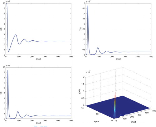
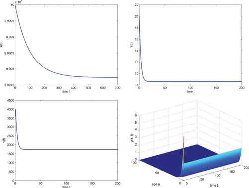
In order to evaluate the effect of cell-to-cell transmission on the virus dynamics, we let ${\beta }_1\left(a\right)=0$ and other parameters remain unchanged. In this case, a direct calculation shows that the basic reproduction number ${\mathcal{R}}_0=18.0506,$ and the endemic steady state becomes $E^{\ast }(9.9977\times {10}^5,2.2665\pi (a),1704.7)$. Comparing Figures 1 and 2, we see that the cell-to-cell transmission can significantly increase the virus load.

Figure 2. The temporal solution found by numerical integration of system (1.4) with the boundary condition (1.5) and initial condition $x\left(0\right)={10}^6$ ml⁻¹, $v\left(0\right)={10}^{-6}$ ml⁻¹, and the parameters $\beta =2.4\times {10}^{-8}$ ml day⁻¹, ${\beta }_1\left(a\right)=0$ ml day⁻¹.

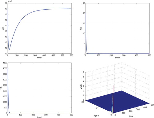
If we choose $\beta =2.4\times {10}^{-10}$ ml day⁻¹, ${\beta }_1\left(a\right)=9\times {10}^{-9}$ ml day⁻¹, then we have the basic reproduction number ${\mathcal{R}}_0=\mathrm{0.2138.}$ By Theorem 4.1, we see that system (4(4) $\begin{array}{rl}& \dot{x}\left(t\right)=s-\mathrm{d}x\left(t\right)-\frac{\beta x\left(t\right)v\left(t\right)}{1+\alpha v\left(t\right)}-x\left(t\right){\int }_0^{\mathrm{\infty }}{\beta }_1\left(a\right)y(a,t)\mathrm{d}a,\\ & \frac{\mathrm{\partial }y(a,t)}{\mathrm{\partial }t}+\frac{\mathrm{\partial }y(a,t)}{\mathrm{\partial }a}=-\mu \left(a\right)y(a,t),\\ & \dot{v}\left(t\right)={\int }_0^{\mathrm{\infty }}k\left(a\right)y(a,t)\mathrm{d}a-uv\left(t\right),\end{array}$(4) ) has only the infection-free steady state $E_1({10}^6,0,0)$ which is locally asymptotically stable. Numerical simulation illustrates this fact (see Figure 3). In Figure 2, $Y\left(t\right)={\int }_0^{300}y(a,t)\mathrm{d}a$.

Figure 3. The temporal solution found by numerical integration of system (4(4) $\begin{array}{rl}& \dot{x}\left(t\right)=s-\mathrm{d}x\left(t\right)-\frac{\beta x\left(t\right)v\left(t\right)}{1+\alpha v\left(t\right)}-x\left(t\right){\int }_0^{\mathrm{\infty }}{\beta }_1\left(a\right)y(a,t)\mathrm{d}a,\\ & \frac{\mathrm{\partial }y(a,t)}{\mathrm{\partial }t}+\frac{\mathrm{\partial }y(a,t)}{\mathrm{\partial }a}=-\mu \left(a\right)y(a,t),\\ & \dot{v}\left(t\right)={\int }_0^{\mathrm{\infty }}k\left(a\right)y(a,t)\mathrm{d}a-uv\left(t\right),\end{array}$(4) ) with the boundary condition (5(5) $y(0,t)=\frac{\beta x\left(t\right)v\left(t\right)}{1+\alpha v\left(t\right)}+x\left(t\right){\int }_0^{\mathrm{\infty }}{\beta }_1\left(a\right)y(a,t)\mathrm{d}a,t>0,$(5) ) and the initial condition $x\left(0\right)={10}^6$ ml⁻¹, $v\left(0\right)={10}^{-6}$ ml⁻¹, and the parameters $\beta =2.4\times {10}^{-10}$ ml day⁻¹, ${\beta }_1\left(a\right)=9\times {10}^{-9}$ ml day⁻¹.

8. Conclusion

In this work, we have investigated an age structured within-host HIV-1 infection model with both virus-to-cell infection and direct cell-to-cell transmission. The model allows the production rate of viral particles and the death rate of productively infected cells to vary and depend on the infection age. By constructing suitable Lyapunov functionals and using LaSalle's invariance principle, it has been shown that global dynamics of system (4(4) $\begin{array}{rl}& \dot{x}\left(t\right)=s-\mathrm{d}x\left(t\right)-\frac{\beta x\left(t\right)v\left(t\right)}{1+\alpha v\left(t\right)}-x\left(t\right){\int }_0^{\mathrm{\infty }}{\beta }_1\left(a\right)y(a,t)\mathrm{d}a,\\ & \frac{\mathrm{\partial }y(a,t)}{\mathrm{\partial }t}+\frac{\mathrm{\partial }y(a,t)}{\mathrm{\partial }a}=-\mu \left(a\right)y(a,t),\\ & \dot{v}\left(t\right)={\int }_0^{\mathrm{\infty }}k\left(a\right)y(a,t)\mathrm{d}a-uv\left(t\right),\end{array}$(4) ) is completely determined by the basic reproduction number. It has been verified that if the basic reproduction number is less than unity, the infection-free steady state is globally asymptotically stable; if the basic reproduction number is greater than unity, the chronic-infection steady state is globally asymptotically stable. The global stability of the chronic-infection steady state rules out any possibility for the existence of Hopf bifurcations and sustained oscillations in system (4(4) $\begin{array}{rl}& \dot{x}\left(t\right)=s-\mathrm{d}x\left(t\right)-\frac{\beta x\left(t\right)v\left(t\right)}{1+\alpha v\left(t\right)}-x\left(t\right){\int }_0^{\mathrm{\infty }}{\beta }_1\left(a\right)y(a,t)\mathrm{d}a,\\ & \frac{\mathrm{\partial }y(a,t)}{\mathrm{\partial }t}+\frac{\mathrm{\partial }y(a,t)}{\mathrm{\partial }a}=-\mu \left(a\right)y(a,t),\\ & \dot{v}\left(t\right)={\int }_0^{\mathrm{\infty }}k\left(a\right)y(a,t)\mathrm{d}a-uv\left(t\right),\end{array}$(4) ).

Disclosure statement

No potential conflict of interest was reported by the authors.

Additional information

Funding

This work was supported by the National Natural Science Foundation of China [No. 11371368] and the Natural Science Foundation of Hebei Province [No. A2014506015].

References

- S. Bonhoeffer, R.M. May, G.M. Shaw, and M.A. Nowak, Virus dynamics and drug therapy, Proc. Natl. Acad. Sci. USA 94 (1997), pp. 6971–6976. doi: 10.1073/pnas.94.13.6971
- P. Chen, W. Hübner, M.A. Spinelli, and B.K. Chen, Predominant mode of human immunodeficiency virus transfer between T cells is mediated by sustained Env-dependent neutralization-resistant virological synapses, J. Virol. 81 (2007), pp. 582–595.
- D. Ebert, C.D. Zschokke-Rohringer, and H.J. Carius, Dose effects and density-dependent regulation of two microparasites of Daphnia magna, Oecologia 122 (2000), pp. 200–209. doi: 10.1007/PL00008847
- J. Feldmann and O. Schwartz, HIV-1 virological synapse: Live imaging of transmission, Viruses 2 (2010), pp. 1666–1680. doi: 10.3390/v2081666
- J.K. Hale and P. Waltman, Persistence in infinite dimensional systems, SIAM J. Math. Anal. 20 (1989), pp. 388–395. doi: 10.1137/0520025
- D.D. Ho, A.U. Neumann, A.S. Perelson, W. Chen, J.M. Leonard, and M. Markowitz, Rapid turnover of plasma virions and CD4+ lymphocytes in HIV-1 infection, Nature 373 (1995), pp. 123–126. doi: 10.1038/373123a0
- G. Huang, X. Liu, and Y. Takeuchi, Lyapunov functions and global stability for age-structured HIV infection model, SIAM J. Appl. Math. 72 (2012), pp. 25–38. doi: 10.1137/110826588
- W. Hübner, G.P. McNerney, P. Chen, B.M. Dale, R.E. Gordon, F.Y.S. Chuang, X.-D. Li, D.M. Asmuth, T. Huser, and B.K. Chen, Quantitative 3D video microscopy of HIV transfer across T cell virological synapses, Science 323 (2009), pp. 1743–1747. doi: 10.1126/science.1167525
- M. Iannelli, Mathematical Theory of Age-Structured Population Dynamics, Applied Mathematics Monographs, Vol. 7, Consiglio Nazionale delle Ricerche (C.N.R), Giardini Pisa, 1995, comitato nazionale per le scienze matematiche.
- N.L. Komarova, D. Anghelina, I. Voznesensky, B. Trinite, D.N. Levy, and D. Wodarz, Relative contribution of free-virus and synaptic transmission to the spread of HIV-1 through target cell populations, Biol. Lett. 9 (2012), pp. 1049–1055. doi: 10.1098/rsbl.2012.1049
- X. Lai and X. Zou, Modeling HIV-1 virus dynamics with both virus-to-cell infection and cell-to-cell transmission, SIAM J. Appl. Math. 74 (2014), pp. 898–917. doi: 10.1137/130930145
- X. Lai and X. Zou, Modeling cell-to-cell spread of HIV-1 with logistic target cell growth, J. Math. Anal. Appl. 426 (2015), pp. 563–584. doi: 10.1016/j.jmaa.2014.10.086
- P. Magal, Compact attractors for time periodic age-structured population models, Electron. J. Differential Equations 2001(65) (2001), pp. 1–35.
- N. Martin and Q. Sattentau, Cell-to-cell HIV-1 spread and its implications for immune evasion, Curr. Opin. HIV AIDS 4 (2009), pp. 143–149. doi: 10.1097/COH.0b013e328322f94a
- P.W. Nelson, M.A. Gilchrist, D. Coombs, J.M. Hyman, and A.S. Perelson, An age-structured model of HIV infection that allows for variations in the production rate of viral particles and the death rate of productively infected cells, Math. Biosci. Eng. 1 (2004), pp. 267–288. doi: 10.3934/mbe.2004.1.267
- M. Nowak and R. May, Virus Dynamics, Oxford University Press, Oxford, 2000.
- M.A. Nowak, R.M. Anderson, M.C. Boerlijst, S. Bonhoeffer, R.M. May, A.J. McMichael, S.M. Wolinsky, K.J. Kunstman, J.T. Safrit, R.A. Koup, A.U. Neumann, and B.T.M. Korber, HIV-1 evolution and disease progression, Science 274 (1996), pp. 1008–1011. doi: 10.1126/science.274.5289.1008
- M.A. Nowak, S. Bonhoeffer, G.M. Shaw, and R.M. May, Anti-viral drug treatment: Dynamics of resistance in free virus and infected cell populations, J. Theoret. Biol. 184 (1997), pp. 203–217. doi: 10.1006/jtbi.1996.0307
- A.S. Perelson and P.W. Nelson, Mathematical analysis of HIV-1 dynamics in vivo, SIAM Rev. 41 (1999), pp. 3–44. doi: 10.1137/S0036144598335107
- A.S. Perelson, D.E. Kirschner, and R. De Boer, Dynamics of HIV infection of CD4+ T cells, Math. Biosci. 114 (1993), pp. 81–125. doi: 10.1016/0025-5564(93)90043-A
- A.S. Perelson, A.U. Neumann, M. Markowitz, J.M. Leonard, and D.D. Ho, HIV-1 dynamics in vivo: Virion clearance rate, infected cell life-span, and viral generation time, Science 271 (1996), pp. 1582–1586. doi: 10.1126/science.271.5255.1582
- R.R. Regoes, D. Ebert, and S. Bonhoeffer, Dose-dependent infection rates of parasites produce the Allee effect in epidemiology, Proc. R. Soc. Lond. B 269 (2002), pp. 271–279. doi: 10.1098/rspb.2001.1816
- C. Reilly, S. Wietgrefe, G. Sedgewick, and A. Haase, Determination of simian immunodeficiency virus production by infected activated and resting cells, AIDS 21 (2007), pp. 163–168. doi: 10.1097/QAD.0b013e328012565b
- L. Rong, Z. Feng, and A.S. Perelson, Mathematical analysis of age-structured HIV-1 dynamics with combination antiretroviral therapy, SIAM J. Appl. Math. 67(3) (2007), pp. 731–756. doi: 10.1137/060663945
- Q. Sattentau, Avoiding the void: Cell-to-cell spread of human viruses, Nat. Rev. Microbiol. 6 (2008), pp. 815–826. doi: 10.1038/nrmicro1972
- Q.J. Sattentau, Cell-to-cell spread of retroviruses, Viruses 2 (2010), pp. 1306–1321. doi: 10.3390/v2061306
- A. Sigal, J.T. Kim, A.B. Balazs, E. Dekel, A. Mayo, R. Milo, and D. Baltimore, Cell-to- cell spread of HIV permits ongoing replication despite antiretroviral therapy, Nature 477 (2011), pp. 95–98. doi: 10.1038/nature10347
- H.L. Smith and H.R. Thieme, Dynamical Systems and Population Persistence, Amer. Math. Soc., Providence, 2011.
- M. Sourisseau, N. Sol-Foulon, F. Porrot, F. Blanchet, and O. Schwartz, Inefficient human immunodeficiency virus replication in mobile lymphocytes, J. Virol. 81 (2007), pp. 1000–1012. doi: 10.1128/JVI.01629-06
- G. Webb, Theory of Nonlinear Age-Dependent Population Dynamics, Marcel Dekker, New York, 1985.