Global dynamics of an epidemiological model with age of infection and disease relapse

ABSTRACT

In this paper, an epidemiological model with age of infection and disease relapse is investigated. The basic reproduction number for the model is identified, and it is shown to be a sharp threshold to completely determine the global dynamics of the model. By analysing the corresponding characteristic equations, the local stability of a disease-free steady state and an endemic steady state of the model is established. By means of suitable Lyapunov functionals and LaSalle's invariance principle, it is verified that if the basic reproduction number is less than unity, the disease-free steady state is globally asymptotically stable, and hence the disease dies out; if the basic reproduction number is greater than unity, the endemic steady state is globally asymptotically stable and the disease becomes endemic.

KEYWORDS:

• Age of infection
• disease relapse
• Lyapunov functional
• LaSalle's invariance principle
• stability

2000 MATHEMATICS SUBJECT CLASSIFICATION:

• 37N25
• 92B05
• 37B25

View correction statement:

Correction

1. Introduction

It is well known that for some diseases, recovered individuals may relapse with reactivation of latent infection and revert back to the infective class. This recurrence of disease is an important feature of some animal and human diseases, for example, tuberculosis (TB), including human and bovine [5,19], and herpes [5,26]. For human TB, incomplete treatment can lead to relapse, but relapse can also occur in patients who took a full course of treatment and were declared cured [25]. Herpes is a human disease that is transmitted by close physical or sexual contact. Important features of herpes are that an individual once infected remains infected for life, and the virus reactivates regularly with reactivation producing a relapse period of infectiousness (see, e.g. [2,14] and references cited therein).

In [22], Tudor formulated the following ordinary differential equation (ODE) compartmental model for herpes: (1) $\begin{array}{rl}\dot{S}\left(t\right)& =A-\mu S\left(t\right)-\beta S\left(t\right)I\left(t\right),\\ \dot{I}\left(t\right)& =\beta S\left(t\right)I\left(t\right)-(\mu +\gamma )I\left(t\right)+\delta R\left(t\right),\\ \dot{R}\left(t\right)& =\gamma I\left(t\right)-(\mu +\delta )R\left(t\right).\end{array}$(1)

In system (1(1) $\begin{array}{rl}\dot{S}\left(t\right)& =A-\mu S\left(t\right)-\beta S\left(t\right)I\left(t\right),\\ \dot{I}\left(t\right)& =\beta S\left(t\right)I\left(t\right)-(\mu +\gamma )I\left(t\right)+\delta R\left(t\right),\\ \dot{R}\left(t\right)& =\gamma I\left(t\right)-(\mu +\delta )R\left(t\right).\end{array}$(1) ), the population is divided into three compartments depending on disease status, where $S\left(t\right)$ represents the number of individuals who are not previously exposed to the virus at time t, $I\left(t\right)$ represents the number of infected individuals who are infectious and are able to spread the disease by contact with susceptible individuals at time t, and $R\left(t\right)$ represents the number of recovered individuals who are previously infected with the virus but not currently shedding virus (latent) at time t. In system (1(1) $\begin{array}{rl}\dot{S}\left(t\right)& =A-\mu S\left(t\right)-\beta S\left(t\right)I\left(t\right),\\ \dot{I}\left(t\right)& =\beta S\left(t\right)I\left(t\right)-(\mu +\gamma )I\left(t\right)+\delta R\left(t\right),\\ \dot{R}\left(t\right)& =\gamma I\left(t\right)-(\mu +\delta )R\left(t\right).\end{array}$(1) ), it is assumed that the population is homogeneous mixing with constant size. The parameter A is the constant birth rate, μ is the death rate, $\beta >0$ is the contact rate, that is, the average number of effective contacts of an infective individual per unit time, and $\gamma >0$ is the rate at which infective individuals recover (latent). It is assumed that an individual in the recovered class can revert to the infective class with a constant rate δ. Here $\delta >0$ implies that the recovered individuals would lose the immunity, and $\delta =0$ implies that the recovered individuals acquire permanent immunity. In [22], the basic reproduction number was identified, and it was shown to be a sharp threshold to determine whether or not the disease dies out or approaches an endemic value. In [20], Moreira and Wang extended system (1(1) $\begin{array}{rl}\dot{S}\left(t\right)& =A-\mu S\left(t\right)-\beta S\left(t\right)I\left(t\right),\\ \dot{I}\left(t\right)& =\beta S\left(t\right)I\left(t\right)-(\mu +\gamma )I\left(t\right)+\delta R\left(t\right),\\ \dot{R}\left(t\right)& =\gamma I\left(t\right)-(\mu +\delta )R\left(t\right).\end{array}$(1) ) to include more general incidence functions, and by using an elementary analysis of Li$\acute{e}$nard's equation and Lyapunov's direct method, and sufficient conditions were established for the global asymptotic stability of the disease-free and endemic equilibria.

There are growing interests in infectious disease models with disease relapse (see, e.g. [1,11,24,25,27,28,30]). In [25], van den Driessche et al. formulated and analysed a model including a general exposed distribution and the possibility of relapse in which a constant exposed period was assumed, for the spread of bovine TB (Mycobacterium bovis) in a cattle herd. For this model with a general probability of remaining in the exposed class, the basic reproduction number was identified and its threshold property was discussed. A model for herpes with a general relapse distribution, but ignoring the exposed class, was formulated in [24] and shown to exhibit a threshold phenomenon.

We note that in model (1(1) $\begin{array}{rl}\dot{S}\left(t\right)& =A-\mu S\left(t\right)-\beta S\left(t\right)I\left(t\right),\\ \dot{I}\left(t\right)& =\beta S\left(t\right)I\left(t\right)-(\mu +\gamma )I\left(t\right)+\delta R\left(t\right),\\ \dot{R}\left(t\right)& =\gamma I\left(t\right)-(\mu +\delta )R\left(t\right).\end{array}$(1) ), infectious individuals are assumed to be equally infectious during their periodic infectivity. However, laboratory studies suggest that the infectivity of infectious individuals be different at the differential age of infection [33]. For TB infection, the TB bacteria need to develop in the lung to be transmissible through coughing, and their transmissibility depends on their progression in the lung as well as the strength of a host's immune system. Active TB has the highest possibility of developing within the first two to five years of infection, while most TB infections remain latent for a long period of time until immune compromise occurs due to ageing or co-infection with other illnesses such as HIV (see, e.g. [6,12,16]). Models with age of infection are often formulated to describe the heterogeneity in infectious individuals.

Recently, great attention has been paid to the modelling and analysis on infectious disease dynamics with age of infection (see, e.g. [3,4,7–10,18,31,32]). In [18], Magal et al. considered an infection-age model of disease transmission with a mass action law incidence, where both the infectiousness and the removal rate may depend on the infection age. A Lyapunov functional was used to prove that the unique endemic steady state is globally stable among solutions for which disease transmission occurs.

Motivated by the works of Magal et al. [18], Tudor [22] and van den Driessche et al. [25], in the present paper, we are concerned with the joint effects of disease relapse and age of infection on the transmission dynamics of infectious diseases. To this end, we consider the following differential equation system: (2) $\begin{array}{rl}& \dot{S}\left(t\right)=A-\mu S\left(t\right)-S\left(t\right){\int }_0^{\mathrm{\infty }}\beta \left(a\right)i(a,t)\mathrm{d}a,\\ & \frac{\mathrm{\partial }i(a,t)}{\mathrm{\partial }t}+\frac{\mathrm{\partial }i(a,t)}{\mathrm{\partial }a}=-(\mu +\gamma (a\left)\right)i(a,t),a>0,\\ & \dot{R}\left(t\right)={\int }_0^{\mathrm{\infty }}\gamma \left(a\right)i(a,t)\mathrm{d}a-(\mu +\delta )R\left(t\right),\end{array}$(2) with the boundary condition (3) $i(0,t)=S\left(t\right){\int }_0^{\mathrm{\infty }}\beta \left(a\right)i(a,t)\mathrm{d}a+\delta R\left(t\right),$(3) and the initial condition (4) $X_0:=\left(S\left(0\right),i(\cdot ,0),R\left(0\right)\right)=\left(S^0,i_0(\cdot ),R^0\right)\in \mathcal{X},$(4) where $\mathcal{X}={\mathbb{R}}^{+}\times L_{+}^1(0,\mathrm{\infty })\times {\mathbb{R}}^{+}$, $L_{+}^1(0,\mathrm{\infty })$ is the set of all integrable functions from $(0,\mathrm{\infty })$ into ${\mathbb{R}}^{+}=[0,\mathrm{\infty })$. In system (2(2) $\begin{array}{rl}& \dot{S}\left(t\right)=A-\mu S\left(t\right)-S\left(t\right){\int }_0^{\mathrm{\infty }}\beta \left(a\right)i(a,t)\mathrm{d}a,\\ & \frac{\mathrm{\partial }i(a,t)}{\mathrm{\partial }t}+\frac{\mathrm{\partial }i(a,t)}{\mathrm{\partial }a}=-(\mu +\gamma (a\left)\right)i(a,t),a>0,\\ & \dot{R}\left(t\right)={\int }_0^{\mathrm{\infty }}\gamma \left(a\right)i(a,t)\mathrm{d}a-(\mu +\delta )R\left(t\right),\end{array}$(2) ), $S\left(t\right)$ represents the number of individuals who are susceptible to the disease, that is, who are not yet infected at time t; $i(a,t)$ represents the density of infected individuals with age of infection a at time t, and $R\left(t\right)$ represents the number of individuals who have been infected and temporarily recovered at time t. Recovery may be natural or due to treatment of infective individuals. The definitions of all parameters in system (2(2) $\begin{array}{rl}& \dot{S}\left(t\right)=A-\mu S\left(t\right)-S\left(t\right){\int }_0^{\mathrm{\infty }}\beta \left(a\right)i(a,t)\mathrm{d}a,\\ & \frac{\mathrm{\partial }i(a,t)}{\mathrm{\partial }t}+\frac{\mathrm{\partial }i(a,t)}{\mathrm{\partial }a}=-(\mu +\gamma (a\left)\right)i(a,t),a>0,\\ & \dot{R}\left(t\right)={\int }_0^{\mathrm{\infty }}\gamma \left(a\right)i(a,t)\mathrm{d}a-(\mu +\delta )R\left(t\right),\end{array}$(2) ) are listed in Table 1.

Table 1. The definition of the parameters in system (2(2) $\begin{array}{rl}& \dot{S}\left(t\right)=A-\mu S\left(t\right)-S\left(t\right){\int }_0^{\mathrm{\infty }}\beta \left(a\right)i(a,t)\mathrm{d}a,\\ & \frac{\mathrm{\partial }i(a,t)}{\mathrm{\partial }t}+\frac{\mathrm{\partial }i(a,t)}{\mathrm{\partial }a}=-(\mu +\gamma (a\left)\right)i(a,t),a>0,\\ & \dot{R}\left(t\right)={\int }_0^{\mathrm{\infty }}\gamma \left(a\right)i(a,t)\mathrm{d}a-(\mu +\delta )R\left(t\right),\end{array}$(2) ).

Parameters	Description
A	Recruitment rate
a	Age of infection, i.e. the time that has lapsed since the individual became infected
μ	Per capita natural death rate
$\beta \left(a\right)$	Transmission coefficient of the infected individuals at age of infection a
$\gamma \left(a\right)$	The rate that an infected individual with age of infection a recovers from the disease
δ	The rate at which an individual in the recovered class reverts to the infective class

In the sequel, we further make the following assumptions:

1. β is Lipschitz continuous on ${\mathbb{R}}^{+}$ with the Lipschitz coefficient $L_{\beta }$.

2. $\beta ,\gamma \in L_{+}^1(0,\mathrm{\infty })$, $\overline{\beta }$ and $\overline{\gamma }$ are the essential supremums of β and γ, respectively.

Using the theory of age-structured dynamical systems developed in [15,29], one can show that system (2(2) $\begin{array}{rl}& \dot{S}\left(t\right)=A-\mu S\left(t\right)-S\left(t\right){\int }_0^{\mathrm{\infty }}\beta \left(a\right)i(a,t)\mathrm{d}a,\\ & \frac{\mathrm{\partial }i(a,t)}{\mathrm{\partial }t}+\frac{\mathrm{\partial }i(a,t)}{\mathrm{\partial }a}=-(\mu +\gamma (a\left)\right)i(a,t),a>0,\\ & \dot{R}\left(t\right)={\int }_0^{\mathrm{\infty }}\gamma \left(a\right)i(a,t)\mathrm{d}a-(\mu +\delta )R\left(t\right),\end{array}$(2) ) has a unique solution $\left(S\right(t),i(a,t),R(t\left)\right)$ satisfying the boundary condition (3(3) $i(0,t)=S\left(t\right){\int }_0^{\mathrm{\infty }}\beta \left(a\right)i(a,t)\mathrm{d}a+\delta R\left(t\right),$(3) ) and the initial condition (4(4) $X_0:=\left(S\left(0\right),i(\cdot ,0),R\left(0\right)\right)=\left(S^0,i_0(\cdot ),R^0\right)\in \mathcal{X},$(4) ). Moreover, it is not difficult to show that all solutions of system (2(2) $\begin{array}{rl}& \dot{S}\left(t\right)=A-\mu S\left(t\right)-S\left(t\right){\int }_0^{\mathrm{\infty }}\beta \left(a\right)i(a,t)\mathrm{d}a,\\ & \frac{\mathrm{\partial }i(a,t)}{\mathrm{\partial }t}+\frac{\mathrm{\partial }i(a,t)}{\mathrm{\partial }a}=-(\mu +\gamma (a\left)\right)i(a,t),a>0,\\ & \dot{R}\left(t\right)={\int }_0^{\mathrm{\infty }}\gamma \left(a\right)i(a,t)\mathrm{d}a-(\mu +\delta )R\left(t\right),\end{array}$(2) ) with the boundary condition (3(3) $i(0,t)=S\left(t\right){\int }_0^{\mathrm{\infty }}\beta \left(a\right)i(a,t)\mathrm{d}a+\delta R\left(t\right),$(3) ) and the initial condition (4(4) $X_0:=\left(S\left(0\right),i(\cdot ,0),R\left(0\right)\right)=\left(S^0,i_0(\cdot ),R^0\right)\in \mathcal{X},$(4) ) are defined on $[0,+\mathrm{\infty })$ and remain positive for all $t\ge 0$. Furthermore, $\mathcal{X}$ is positively invariant and system (2(2) $\begin{array}{rl}& \dot{S}\left(t\right)=A-\mu S\left(t\right)-S\left(t\right){\int }_0^{\mathrm{\infty }}\beta \left(a\right)i(a,t)\mathrm{d}a,\\ & \frac{\mathrm{\partial }i(a,t)}{\mathrm{\partial }t}+\frac{\mathrm{\partial }i(a,t)}{\mathrm{\partial }a}=-(\mu +\gamma (a\left)\right)i(a,t),a>0,\\ & \dot{R}\left(t\right)={\int }_0^{\mathrm{\infty }}\gamma \left(a\right)i(a,t)\mathrm{d}a-(\mu +\delta )R\left(t\right),\end{array}$(2) ) exhibits a continuous semi-flow $\mathrm{\Phi }:{\mathbb{R}}^{+}\times \mathcal{X}\to \mathcal{X}$, namely, (5) ${\mathrm{\Phi }}_t\left(X_0\right)=\mathrm{\Phi }(t,X_0):=\left(S\left(t\right),i(\cdot ,t),R\left(t\right)\right),t\ge 0,X_0\in \mathcal{X}.$(5) Given a point $(x,\varphi ,z)\in \mathcal{X}$, we have the norm $\parallel (x,\varphi ,z){\parallel }_{\mathcal{X}}:=x+{\int }_0^{\mathrm{\infty }}\varphi \left(a\right)\mathrm{d}a+z.$ The analysis of the global stability of infectious disease models with infection age has been a much more interesting topic recently from realistic views to theoretical views. The primary goal of this work is to carry out a complete mathematical analysis of system (2(2) $\begin{array}{rl}& \dot{S}\left(t\right)=A-\mu S\left(t\right)-S\left(t\right){\int }_0^{\mathrm{\infty }}\beta \left(a\right)i(a,t)\mathrm{d}a,\\ & \frac{\mathrm{\partial }i(a,t)}{\mathrm{\partial }t}+\frac{\mathrm{\partial }i(a,t)}{\mathrm{\partial }a}=-(\mu +\gamma (a\left)\right)i(a,t),a>0,\\ & \dot{R}\left(t\right)={\int }_0^{\mathrm{\infty }}\gamma \left(a\right)i(a,t)\mathrm{d}a-(\mu +\delta )R\left(t\right),\end{array}$(2) ) with the boundary condition (3(3) $i(0,t)=S\left(t\right){\int }_0^{\mathrm{\infty }}\beta \left(a\right)i(a,t)\mathrm{d}a+\delta R\left(t\right),$(3) ) and the initial condition (4(4) $X_0:=\left(S\left(0\right),i(\cdot ,0),R\left(0\right)\right)=\left(S^0,i_0(\cdot ),R^0\right)\in \mathcal{X},$(4) ), and establish its global dynamics. The organization of this paper is as follows. In the next section, in order to study the global dynamics, we are concerned with the asymptotic smoothness of the semi-flow generated by system (2(2) $\begin{array}{rl}& \dot{S}\left(t\right)=A-\mu S\left(t\right)-S\left(t\right){\int }_0^{\mathrm{\infty }}\beta \left(a\right)i(a,t)\mathrm{d}a,\\ & \frac{\mathrm{\partial }i(a,t)}{\mathrm{\partial }t}+\frac{\mathrm{\partial }i(a,t)}{\mathrm{\partial }a}=-(\mu +\gamma (a\left)\right)i(a,t),a>0,\\ & \dot{R}\left(t\right)={\int }_0^{\mathrm{\infty }}\gamma \left(a\right)i(a,t)\mathrm{d}a-(\mu +\delta )R\left(t\right),\end{array}$(2) ). In Section 3, we calculate the basic reproduction number and establish the existence of feasible steady states of system (2(2) $\begin{array}{rl}& \dot{S}\left(t\right)=A-\mu S\left(t\right)-S\left(t\right){\int }_0^{\mathrm{\infty }}\beta \left(a\right)i(a,t)\mathrm{d}a,\\ & \frac{\mathrm{\partial }i(a,t)}{\mathrm{\partial }t}+\frac{\mathrm{\partial }i(a,t)}{\mathrm{\partial }a}=-(\mu +\gamma (a\left)\right)i(a,t),a>0,\\ & \dot{R}\left(t\right)={\int }_0^{\mathrm{\infty }}\gamma \left(a\right)i(a,t)\mathrm{d}a-(\mu +\delta )R\left(t\right),\end{array}$(2) ) with the boundary condition (3(3) $i(0,t)=S\left(t\right){\int }_0^{\mathrm{\infty }}\beta \left(a\right)i(a,t)\mathrm{d}a+\delta R\left(t\right),$(3) ). In Section 4, by analysing corresponding characteristic equations, we study the local asymptotic stability of a disease-free steady state and an endemic steady state of system (2(2) $\begin{array}{rl}& \dot{S}\left(t\right)=A-\mu S\left(t\right)-S\left(t\right){\int }_0^{\mathrm{\infty }}\beta \left(a\right)i(a,t)\mathrm{d}a,\\ & \frac{\mathrm{\partial }i(a,t)}{\mathrm{\partial }t}+\frac{\mathrm{\partial }i(a,t)}{\mathrm{\partial }a}=-(\mu +\gamma (a\left)\right)i(a,t),a>0,\\ & \dot{R}\left(t\right)={\int }_0^{\mathrm{\infty }}\gamma \left(a\right)i(a,t)\mathrm{d}a-(\mu +\delta )R\left(t\right),\end{array}$(2) ). In Section 5, by using the persistence theory for infinite system developed by Hale and Waltman [13], we verify that if the endemic steady state exists, then system (2(2) $\begin{array}{rl}& \dot{S}\left(t\right)=A-\mu S\left(t\right)-S\left(t\right){\int }_0^{\mathrm{\infty }}\beta \left(a\right)i(a,t)\mathrm{d}a,\\ & \frac{\mathrm{\partial }i(a,t)}{\mathrm{\partial }t}+\frac{\mathrm{\partial }i(a,t)}{\mathrm{\partial }a}=-(\mu +\gamma (a\left)\right)i(a,t),a>0,\\ & \dot{R}\left(t\right)={\int }_0^{\mathrm{\infty }}\gamma \left(a\right)i(a,t)\mathrm{d}a-(\mu +\delta )R\left(t\right),\end{array}$(2) ) is uniformly persistent. In Section 6, we study the global stability of each of feasible steady states of system (2(2) $\begin{array}{rl}& \dot{S}\left(t\right)=A-\mu S\left(t\right)-S\left(t\right){\int }_0^{\mathrm{\infty }}\beta \left(a\right)i(a,t)\mathrm{d}a,\\ & \frac{\mathrm{\partial }i(a,t)}{\mathrm{\partial }t}+\frac{\mathrm{\partial }i(a,t)}{\mathrm{\partial }a}=-(\mu +\gamma (a\left)\right)i(a,t),a>0,\\ & \dot{R}\left(t\right)={\int }_0^{\mathrm{\infty }}\gamma \left(a\right)i(a,t)\mathrm{d}a-(\mu +\delta )R\left(t\right),\end{array}$(2) ) by means of Lyapunov functionals and LaSalle's invariance principle. Numerical simulations are carried out in Section 7 to illustrate the theoretical results. A brief discussion is given in Section 8 to conclude this work.

2. Asymptotic smoothness

In order to study the global dynamics of system (2(2) $\begin{array}{rl}& \dot{S}\left(t\right)=A-\mu S\left(t\right)-S\left(t\right){\int }_0^{\mathrm{\infty }}\beta \left(a\right)i(a,t)\mathrm{d}a,\\ & \frac{\mathrm{\partial }i(a,t)}{\mathrm{\partial }t}+\frac{\mathrm{\partial }i(a,t)}{\mathrm{\partial }a}=-(\mu +\gamma (a\left)\right)i(a,t),a>0,\\ & \dot{R}\left(t\right)={\int }_0^{\mathrm{\infty }}\gamma \left(a\right)i(a,t)\mathrm{d}a-(\mu +\delta )R\left(t\right),\end{array}$(2) ), we need to show the asymptotic smoothness of the semi-flow $\left\{\mathrm{\Phi }\right(t){\}}_{t\ge 0}$ generated by system (2(2) $\begin{array}{rl}& \dot{S}\left(t\right)=A-\mu S\left(t\right)-S\left(t\right){\int }_0^{\mathrm{\infty }}\beta \left(a\right)i(a,t)\mathrm{d}a,\\ & \frac{\mathrm{\partial }i(a,t)}{\mathrm{\partial }t}+\frac{\mathrm{\partial }i(a,t)}{\mathrm{\partial }a}=-(\mu +\gamma (a\left)\right)i(a,t),a>0,\\ & \dot{R}\left(t\right)={\int }_0^{\mathrm{\infty }}\gamma \left(a\right)i(a,t)\mathrm{d}a-(\mu +\delta )R\left(t\right),\end{array}$(2) ).

2.1. Boundedness of solutions

In this section, we show the boundedness of solutions of system (2(2) $\begin{array}{rl}& \dot{S}\left(t\right)=A-\mu S\left(t\right)-S\left(t\right){\int }_0^{\mathrm{\infty }}\beta \left(a\right)i(a,t)\mathrm{d}a,\\ & \frac{\mathrm{\partial }i(a,t)}{\mathrm{\partial }t}+\frac{\mathrm{\partial }i(a,t)}{\mathrm{\partial }a}=-(\mu +\gamma (a\left)\right)i(a,t),a>0,\\ & \dot{R}\left(t\right)={\int }_0^{\mathrm{\infty }}\gamma \left(a\right)i(a,t)\mathrm{d}a-(\mu +\delta )R\left(t\right),\end{array}$(2) ) with the boundary condition (3(3) $i(0,t)=S\left(t\right){\int }_0^{\mathrm{\infty }}\beta \left(a\right)i(a,t)\mathrm{d}a+\delta R\left(t\right),$(3) ) and the initial condition (4(4) $X_0:=\left(S\left(0\right),i(\cdot ,0),R\left(0\right)\right)=\left(S^0,i_0(\cdot ),R^0\right)\in \mathcal{X},$(4) ).

Proposition 2.1

Let ${\mathrm{\Phi }}_t$ be defined as in Equation (5(5) ${\mathrm{\Phi }}_t\left(X_0\right)=\mathrm{\Phi }(t,X_0):=\left(S\left(t\right),i(\cdot ,t),R\left(t\right)\right),t\ge 0,X_0\in \mathcal{X}.$(5) ). Then the following statements hold.

1. $\left(\mathrm{d}/\mathrm{d}t\right)\parallel {\mathrm{\Phi }}_t\left(X_0\right){\parallel }_{\mathcal{X}}\le A-\mu \parallel {\mathrm{\Phi }}_t\left(X_0\right){\parallel }_{\mathcal{X}}$ for all $t\ge 0;$

2. $\parallel {\mathrm{\Phi }}_t\left(X_0\right){\parallel }_{\mathcal{X}}\le max\{A/\mu ,\parallel X_0{\parallel }_{\mathcal{X}}\}$ for all $t\ge 0;$

3. $\underset{t\to +\mathrm{\infty }}{lim sup}\parallel {\mathrm{\Phi }}_t\left(X_0\right){\parallel }_{\mathcal{X}}\le A/\mu ;$

4. ${\mathrm{\Phi }}_t$ is point dissipative: there is a bounded set that attracts all points in $\mathcal{X}$.

Proof.

Let ${\mathrm{\Phi }}_t\left(X_0\right)=\mathrm{\Phi }(t,X_0):=\left(S\right(t),i(\cdot ,t),R(t\left)\right)$ be any nonnegative solution of system (2(2) $\begin{array}{rl}& \dot{S}\left(t\right)=A-\mu S\left(t\right)-S\left(t\right){\int }_0^{\mathrm{\infty }}\beta \left(a\right)i(a,t)\mathrm{d}a,\\ & \frac{\mathrm{\partial }i(a,t)}{\mathrm{\partial }t}+\frac{\mathrm{\partial }i(a,t)}{\mathrm{\partial }a}=-(\mu +\gamma (a\left)\right)i(a,t),a>0,\\ & \dot{R}\left(t\right)={\int }_0^{\mathrm{\infty }}\gamma \left(a\right)i(a,t)\mathrm{d}a-(\mu +\delta )R\left(t\right),\end{array}$(2) ) with the boundary condition (3(3) $i(0,t)=S\left(t\right){\int }_0^{\mathrm{\infty }}\beta \left(a\right)i(a,t)\mathrm{d}a+\delta R\left(t\right),$(3) ) and the initial condition (4(4) $X_0:=\left(S\left(0\right),i(\cdot ,0),R\left(0\right)\right)=\left(S^0,i_0(\cdot ),R^0\right)\in \mathcal{X},$(4) ). Denote $\parallel X_0{\parallel }_{\mathcal{X}}=S^0+{\int }_0^{\mathrm{\infty }}{i}_0\left(a\right)da+R^0$.

Define (6) $\parallel \mathrm{\Phi }(t,X_0){\parallel }_{\mathcal{X}}=S\left(t\right)+{\int }_0^{\mathrm{\infty }}i(a,t)\mathrm{d}a+R\left(t\right).$(6) It follows from system (2(2) $\begin{array}{rl}& \dot{S}\left(t\right)=A-\mu S\left(t\right)-S\left(t\right){\int }_0^{\mathrm{\infty }}\beta \left(a\right)i(a,t)\mathrm{d}a,\\ & \frac{\mathrm{\partial }i(a,t)}{\mathrm{\partial }t}+\frac{\mathrm{\partial }i(a,t)}{\mathrm{\partial }a}=-(\mu +\gamma (a\left)\right)i(a,t),a>0,\\ & \dot{R}\left(t\right)={\int }_0^{\mathrm{\infty }}\gamma \left(a\right)i(a,t)\mathrm{d}a-(\mu +\delta )R\left(t\right),\end{array}$(2) ) that (7) $\begin{array}{rl}\frac{\mathrm{d}}{\mathrm{d}t}\parallel \mathrm{\Phi }(t,X_0){\parallel }_{\mathcal{X}}& =A-\mu S\left(t\right)-S\left(t\right){\int }_0^{\mathrm{\infty }}\beta \left(a\right)i(a,t)\mathrm{d}a\\ & +{\int }_0^{\mathrm{\infty }}\frac{\mathrm{\partial }i(a,t)}{\mathrm{\partial }t}\mathrm{d}a+{\int }_0^{\mathrm{\infty }}\gamma \left(a\right)i(a,t)\mathrm{d}a-(\mu +\delta )R\left(t\right).\end{array}$(7) On substituting $\mathrm{\partial }i(a,t)/\mathrm{\partial }t+\mathrm{\partial }i(a,t)/\mathrm{\partial }a=-(\mu +\gamma (a\left)\right)i(a,t)$ into Equation (7(7) $\begin{array}{rl}\frac{\mathrm{d}}{\mathrm{d}t}\parallel \mathrm{\Phi }(t,X_0){\parallel }_{\mathcal{X}}& =A-\mu S\left(t\right)-S\left(t\right){\int }_0^{\mathrm{\infty }}\beta \left(a\right)i(a,t)\mathrm{d}a\\ & +{\int }_0^{\mathrm{\infty }}\frac{\mathrm{\partial }i(a,t)}{\mathrm{\partial }t}\mathrm{d}a+{\int }_0^{\mathrm{\infty }}\gamma \left(a\right)i(a,t)\mathrm{d}a-(\mu +\delta )R\left(t\right).\end{array}$(7) ), we obtain that (8) $\begin{array}{rl}\frac{\mathrm{d}}{\mathrm{d}t}\parallel \mathrm{\Phi }(t,X_0){\parallel }_{\mathcal{X}}& =A-\mu S\left(t\right)-S\left(t\right){\int }_0^{\mathrm{\infty }}\beta \left(a\right)i(a,t)\mathrm{d}a\\ & -{\int }_0^{\mathrm{\infty }}\frac{\mathrm{\partial }i(a,t)}{\mathrm{\partial }a}\mathrm{d}a-{\int }_0^{\mathrm{\infty }}\nu \left(a\right)i(a,t)\mathrm{d}a\\ & +{\int }_0^{\mathrm{\infty }}\gamma \left(a\right)i(a,t)\mathrm{d}a-(\mu +\delta )R\left(t\right)\\ & =A-\mu S\left(t\right)-S\left(t\right){\int }_0^{\mathrm{\infty }}\beta \left(a\right)i(a,t)\mathrm{d}a\\ & -i(a,t){|}_0^{\mathrm{\infty }}-{\int }_0^{\mathrm{\infty }}(\mu +\gamma (a\left)\right)i(a,t)\mathrm{d}a\\ & +{\int }_0^{\mathrm{\infty }}\gamma \left(a\right)i(a,t)\mathrm{d}a-(\mu +\delta )R\left(t\right).\end{array}$(8) It follows from Equations (3(3) $i(0,t)=S\left(t\right){\int }_0^{\mathrm{\infty }}\beta \left(a\right)i(a,t)\mathrm{d}a+\delta R\left(t\right),$(3) ) and (8(8) $\begin{array}{rl}\frac{\mathrm{d}}{\mathrm{d}t}\parallel \mathrm{\Phi }(t,X_0){\parallel }_{\mathcal{X}}& =A-\mu S\left(t\right)-S\left(t\right){\int }_0^{\mathrm{\infty }}\beta \left(a\right)i(a,t)\mathrm{d}a\\ & -{\int }_0^{\mathrm{\infty }}\frac{\mathrm{\partial }i(a,t)}{\mathrm{\partial }a}\mathrm{d}a-{\int }_0^{\mathrm{\infty }}\nu \left(a\right)i(a,t)\mathrm{d}a\\ & +{\int }_0^{\mathrm{\infty }}\gamma \left(a\right)i(a,t)\mathrm{d}a-(\mu +\delta )R\left(t\right)\\ & =A-\mu S\left(t\right)-S\left(t\right){\int }_0^{\mathrm{\infty }}\beta \left(a\right)i(a,t)\mathrm{d}a\\ & -i(a,t){|}_0^{\mathrm{\infty }}-{\int }_0^{\mathrm{\infty }}(\mu +\gamma (a\left)\right)i(a,t)\mathrm{d}a\\ & +{\int }_0^{\mathrm{\infty }}\gamma \left(a\right)i(a,t)\mathrm{d}a-(\mu +\delta )R\left(t\right).\end{array}$(8) ) that (9) $\begin{array}{rl}\frac{\mathrm{d}}{\mathrm{d}t}\parallel \mathrm{\Phi }(t,X_0){\parallel }_{\mathcal{X}}& \le A-\mu S\left(t\right)-\mu {\int }_0^{\mathrm{\infty }}i(a,t)\mathrm{d}a-\mu R\left(t\right)\\ & =A-\mu \parallel \mathrm{\Phi }(t,X_0){\parallel }_{\mathcal{X}}.\end{array}$(9) The variation of constants formula implies $\parallel \mathrm{\Phi }(t,X_0){\parallel }_{\mathcal{X}}\le \frac{A}{\mu }-{\mathrm{e}}^{-\mu t}\left\{\frac{A}{\mu }-\parallel X_0{\parallel }_{\mathcal{X}}\right\},$ which yields $\parallel \mathrm{\Phi }(t,X_0){\parallel }_{\mathcal{X}}\le max\left\{\frac{A}{\mu },\parallel X_0{\parallel }_{\mathcal{X}}\right\},$ for all $t\ge 0$. This completes the proof.

The following results are direct consequences of Proposition 2.1.

Proposition 2.2

If $X_0\in \mathcal{X}$ and $\parallel X_0{\parallel }_{\mathcal{X}}\le K$ for some $K\ge A/\mu ,$ then (10) $S\left(t\right)\le K,{\int }_0^{\mathrm{\infty }}i(a,t)\mathrm{d}a\le K,R\left(t\right)\le K,$(10) for all $t\ge 0$.

Proposition 2.3

Let $C\in \mathcal{X}$ be bounded. Then

1. ${\mathrm{\Phi }}_t\left(C\right)$ is bounded;

2. ${\mathrm{\Phi }}_t$ is eventually bounded on C.

2.2. Asymptotic smoothness

In this section, we are concerned with the asymptotic smoothness of the semi-flow Φ generated by system (2(2) $\begin{array}{rl}& \dot{S}\left(t\right)=A-\mu S\left(t\right)-S\left(t\right){\int }_0^{\mathrm{\infty }}\beta \left(a\right)i(a,t)\mathrm{d}a,\\ & \frac{\mathrm{\partial }i(a,t)}{\mathrm{\partial }t}+\frac{\mathrm{\partial }i(a,t)}{\mathrm{\partial }a}=-(\mu +\gamma (a\left)\right)i(a,t),a>0,\\ & \dot{R}\left(t\right)={\int }_0^{\mathrm{\infty }}\gamma \left(a\right)i(a,t)\mathrm{d}a-(\mu +\delta )R\left(t\right),\end{array}$(2) ).

Let $\left(S\right(t),i(\cdot ,t),R(t\left)\right)$ be a solution of system (2(2) $\begin{array}{rl}& \dot{S}\left(t\right)=A-\mu S\left(t\right)-S\left(t\right){\int }_0^{\mathrm{\infty }}\beta \left(a\right)i(a,t)\mathrm{d}a,\\ & \frac{\mathrm{\partial }i(a,t)}{\mathrm{\partial }t}+\frac{\mathrm{\partial }i(a,t)}{\mathrm{\partial }a}=-(\mu +\gamma (a\left)\right)i(a,t),a>0,\\ & \dot{R}\left(t\right)={\int }_0^{\mathrm{\infty }}\gamma \left(a\right)i(a,t)\mathrm{d}a-(\mu +\delta )R\left(t\right),\end{array}$(2) ) with the boundary condition (3(3) $i(0,t)=S\left(t\right){\int }_0^{\mathrm{\infty }}\beta \left(a\right)i(a,t)\mathrm{d}a+\delta R\left(t\right),$(3) ) and the initial condition (4(4) $X_0:=\left(S\left(0\right),i(\cdot ,0),R\left(0\right)\right)=\left(S^0,i_0(\cdot ),R^0\right)\in \mathcal{X},$(4) ). Integrating the second equation of system (2(2) $\begin{array}{rl}& \dot{S}\left(t\right)=A-\mu S\left(t\right)-S\left(t\right){\int }_0^{\mathrm{\infty }}\beta \left(a\right)i(a,t)\mathrm{d}a,\\ & \frac{\mathrm{\partial }i(a,t)}{\mathrm{\partial }t}+\frac{\mathrm{\partial }i(a,t)}{\mathrm{\partial }a}=-(\mu +\gamma (a\left)\right)i(a,t),a>0,\\ & \dot{R}\left(t\right)={\int }_0^{\mathrm{\infty }}\gamma \left(a\right)i(a,t)\mathrm{d}a-(\mu +\delta )R\left(t\right),\end{array}$(2) ) along the characteristic line $t-a=\mathrm{const}.$, we have (11) $i(a,t)=\left\{\begin{array}{ll}L(t-a)\phi \left(a\right),& 0\le a<t,\\ i_0(a-t)\frac{\phi \left(a\right)}{\phi (a-t)},& 0\le t\le a,\end{array}\right.$(11) where (12) $L\left(t\right)=S\left(t\right)A\left(t\right),A\left(t\right)={\int }_0^{\mathrm{\infty }}\beta \left(a\right)i(a,t)\mathrm{d}a,$(12) and (13) $\phi \left(a\right)={\mathrm{e}}^{-{\int }_0^a(\mu +\gamma (s\left)\right)\mathrm{d}s}.$(13)

Proposition 2.4

The functions $A\left(t\right)$ is Lipschitz continuous on ${\mathbb{R}}^{+}$.

Proof.

Let $K\ge max\{A/\mu ,\parallel X_0{\parallel }_{\mathcal{X}}\}$. By Proposition 2.1 we have $\parallel {\mathrm{\Phi }}_t{\parallel }_{\mathcal{X}}\le K$ for all $t\ge 0$.

Fix $t\ge 0$ and h>0. Then (14) $\begin{array}{rl}A(t+h)-A\left(t\right)& ={\int }_0^{\mathrm{\infty }}\beta \left(a\right)i(a,t+h)\mathrm{d}a-{\int }_0^{\mathrm{\infty }}\beta \left(a\right)i(a,t)\mathrm{d}a\\ & ={\int }_0^h\beta \left(a\right)i(a,t+h)\mathrm{d}a+{\int }_h^{\mathrm{\infty }}\beta \left(a\right)i(a,t+h)\mathrm{d}a\\ & -{\int }_0^{\mathrm{\infty }}\beta \left(a\right)i(a,t)\mathrm{d}a.\end{array}$(14) On substituting Equation (11(11) $i(a,t)=\left\{\begin{array}{ll}L(t-a)\phi \left(a\right),& 0\le a<t,\\ i_0(a-t)\frac{\phi \left(a\right)}{\phi (a-t)},& 0\le t\le a,\end{array}\right.$(11) ) into Equation (14(14) $\begin{array}{rl}A(t+h)-A\left(t\right)& ={\int }_0^{\mathrm{\infty }}\beta \left(a\right)i(a,t+h)\mathrm{d}a-{\int }_0^{\mathrm{\infty }}\beta \left(a\right)i(a,t)\mathrm{d}a\\ & ={\int }_0^h\beta \left(a\right)i(a,t+h)\mathrm{d}a+{\int }_h^{\mathrm{\infty }}\beta \left(a\right)i(a,t+h)\mathrm{d}a\\ & -{\int }_0^{\mathrm{\infty }}\beta \left(a\right)i(a,t)\mathrm{d}a.\end{array}$(14) ), we have (15) $\begin{array}{rl}A(t+h)-A\left(t\right)& ={\int }_0^h\beta \left(a\right)L(t+h-a)\phi \left(a\right)\mathrm{d}a\\ & +{\int }_h^{\mathrm{\infty }}\beta \left(a\right)i(a,t+h)\mathrm{d}a-{\int }_0^{\mathrm{\infty }}\beta \left(a\right)i(a,t)\mathrm{d}a.\end{array}$(15) By Proposition 2.2, we have $L\left(t\right)\le \overline{\beta }{K}^2$. Noting that $\phi \left(a\right)\le 1$, it follows from Equation (15(15) $\begin{array}{rl}A(t+h)-A\left(t\right)& ={\int }_0^h\beta \left(a\right)L(t+h-a)\phi \left(a\right)\mathrm{d}a\\ & +{\int }_h^{\mathrm{\infty }}\beta \left(a\right)i(a,t+h)\mathrm{d}a-{\int }_0^{\mathrm{\infty }}\beta \left(a\right)i(a,t)\mathrm{d}a.\end{array}$(15) ) that (16) $\begin{array}{rl}\left|A(t+h)-A\left(t\right)\right|& \le \overline{\beta }{K}^{2}h+\left|{\int }_h^{\mathrm{\infty }}\beta \left(a\right)i(a,t+h)\mathrm{d}a-{\int }_0^{\mathrm{\infty }}\beta \left(a\right)i(a,t)\mathrm{d}a\right|\\ & =\overline{\beta }{K}^{2}h+\left|{\int }_0^{\mathrm{\infty }}\beta (\sigma +h)i(\sigma +h,t+h)\mathrm{d}\sigma -{\int }_0^{\mathrm{\infty }}\beta \left(a\right)i(a,t)\mathrm{d}a\right|.\end{array}$(16) We derive from Equation (11(11) $i(a,t)=\left\{\begin{array}{ll}L(t-a)\phi \left(a\right),& 0\le a<t,\\ i_0(a-t)\frac{\phi \left(a\right)}{\phi (a-t)},& 0\le t\le a,\end{array}\right.$(11) ) that (17) $i(a+h,t+h)=i(a,t)\frac{\phi (a+h)}{\phi \left(a\right)}=i(a,t){\mathrm{e}}^{-{\int }_a^{a+h}(\mu +\gamma (s\left)\right)\mathrm{d}s},$(17) for all $a\ge 0,t\ge 0,h\ge 0$. Hence, Equation (16(16) $\begin{array}{rl}\left|A(t+h)-A\left(t\right)\right|& \le \overline{\beta }{K}^{2}h+\left|{\int }_h^{\mathrm{\infty }}\beta \left(a\right)i(a,t+h)\mathrm{d}a-{\int }_0^{\mathrm{\infty }}\beta \left(a\right)i(a,t)\mathrm{d}a\right|\\ & =\overline{\beta }{K}^{2}h+\left|{\int }_0^{\mathrm{\infty }}\beta (\sigma +h)i(\sigma +h,t+h)\mathrm{d}\sigma -{\int }_0^{\mathrm{\infty }}\beta \left(a\right)i(a,t)\mathrm{d}a\right|.\end{array}$(16) ) can be rewritten as (18) $\begin{array}{rl}\left|A(t+h)-A\left(t\right)\right|& \le \overline{\beta }{K}^{2}h+\left|{\int }_0^{\mathrm{\infty }}\beta (a+h)i(a,t){\mathrm{e}}^{-{\int }_a^{a+h}(\mu +\gamma (s\left)\right)\mathrm{d}s}\mathrm{d}a\right.\\ & \left.-{\int }_0^{\mathrm{\infty }}\beta \left(a\right)i(a,t)\mathrm{d}a\right|\\ & \le \overline{\beta }{K}^{2}h+{\int }_0^{\mathrm{\infty }}\beta (a+h)\left(1-{\mathrm{e}}^{-{\int }_a^{a+h}(\mu +\gamma (s\left)\right)\mathrm{d}s}\right)i(a,t)\mathrm{d}a\\ & +{\int }_0^{\mathrm{\infty }}\left|\beta (a+h)-\beta \left(a\right)\right|i(a,t)\mathrm{d}a.\end{array}$(18) Noting that $1-{\mathrm{e}}^{-x}\le x$ for $x\ge 0$, it follows from Equation (18(18) $\begin{array}{rl}\left|A(t+h)-A\left(t\right)\right|& \le \overline{\beta }{K}^{2}h+\left|{\int }_0^{\mathrm{\infty }}\beta (a+h)i(a,t){\mathrm{e}}^{-{\int }_a^{a+h}(\mu +\gamma (s\left)\right)\mathrm{d}s}\mathrm{d}a\right.\\ & \left.-{\int }_0^{\mathrm{\infty }}\beta \left(a\right)i(a,t)\mathrm{d}a\right|\\ & \le \overline{\beta }{K}^{2}h+{\int }_0^{\mathrm{\infty }}\beta (a+h)\left(1-{\mathrm{e}}^{-{\int }_a^{a+h}(\mu +\gamma (s\left)\right)\mathrm{d}s}\right)i(a,t)\mathrm{d}a\\ & +{\int }_0^{\mathrm{\infty }}\left|\beta (a+h)-\beta \left(a\right)\right|i(a,t)\mathrm{d}a.\end{array}$(18) ) that (19) $\left|A(t+h)-A\left(t\right)\right|\le K[\overline{\beta }K+\overline{\beta }(\mu +\overline{\gamma })+L_{\beta }]h,$(19) here the fact that $\beta \left(a\right)$ is Lipschitz continuous on ${\mathbb{R}}^{+}$ was used. This completes the proof.

Proposition 2.5

The function $L\left(t\right)$ is Lipschitz continuous on ${\mathbb{R}}^{+}$.

Proof.

Let $K\ge max\{A/\mu ,\parallel X_0{\parallel }_{\mathcal{X}}\}$. By Proposition 2.1, we have $\parallel {\mathrm{\Phi }}_t{\parallel }_{\mathcal{X}}\le K$ for all $t\ge 0$.

Fix $t\ge 0$ and h>0. Then (20) $\begin{array}{rl}\left|L(t+h)-L\left(t\right)\right|& \le A(t+h)\left|S(t+h)-S\left(t\right)\right|+S\left(t\right)\left|A(t+h)-A\left(t\right)\right|\\ & \le M_{L}h,\end{array}$(20) where (21) $M_L=\overline{\beta }K\left(A+\mu K+\overline{\beta }{K}^2\right)+K^2\left[\overline{\beta }\right(\mu +\overline{\gamma }+K)+L_{\beta }].$(21) This completes the proof.

In order to prove the asymptotic smoothness of the semi-flow Φ generated by system (2(2) $\begin{array}{rl}& \dot{S}\left(t\right)=A-\mu S\left(t\right)-S\left(t\right){\int }_0^{\mathrm{\infty }}\beta \left(a\right)i(a,t)\mathrm{d}a,\\ & \frac{\mathrm{\partial }i(a,t)}{\mathrm{\partial }t}+\frac{\mathrm{\partial }i(a,t)}{\mathrm{\partial }a}=-(\mu +\gamma (a\left)\right)i(a,t),a>0,\\ & \dot{R}\left(t\right)={\int }_0^{\mathrm{\infty }}\gamma \left(a\right)i(a,t)\mathrm{d}a-(\mu +\delta )R\left(t\right),\end{array}$(2) ), we introduce the following theorems (Theorems 2.46 and B.2 in [21]).

Theorem 2.1

The semi-flow $\mathrm{\Phi }:{\mathbb{R}}^{+}\times {\mathcal{X}}_{+}\to {\mathcal{X}}_{+}$ is asymptotically smooth if there are maps $\mathrm{\Theta },\mathrm{\Psi }:{\mathbb{R}}^{+}\times {\mathcal{X}}_{+}\to {\mathcal{X}}_{+}$ such that $\mathrm{\Phi }(t,X)=\mathrm{\Theta }(t,X)+\mathrm{\Psi }(t,X)$ and the following conditions hold for any bounded closed set $\mathcal{C}\subset {\mathcal{X}}_{+}$ that is forward invariant under Φ:

1. $\underset{t\to +\mathrm{\infty }}{lim}\mathrm{diam}\mathrm{\Theta }(t,\mathcal{C})=0;$

2. there exists $t_{\mathcal{C}}\ge 0$ such that $\mathrm{\Psi }(t,\mathcal{C})$ has compact closure for each $t\ge t_{\mathcal{C}}$.

Theorem 2.2

Let $\mathcal{C}$ be a subset of $L^1\left({\mathbb{R}}^{+}\right)$. Then $\mathcal{C}$ has compact closure if and only if the following assumptions hold:

1. $\underset{f\in \mathcal{C}}{sup}{\int }_0^{\mathrm{\infty }}|f\left(a\right)|\mathrm{d}a<\mathrm{\infty };$

2. $\underset{r\to \mathrm{\infty }}{lim}{\int }_r^{\mathrm{\infty }}|f\left(a\right)|\mathrm{d}a=0$ uniformly in $f\in \mathcal{C};$

3. $\underset{h\to 0^{+}}{lim}{\int }_0^{\mathrm{\infty }}|f(a+h)-f\left(a\right)|\mathrm{d}a=0$ uniformly in $f\in \mathcal{C};$

4. $\underset{h\to 0^{+}}{lim}{\int }_0^h|f\left(a\right)|\mathrm{d}a=0$ uniformly in $f\in \mathcal{C}$.

We are now in a position to state and prove a result on the asymptotic smoothness of the semi-flow Φ generated by system (2(2) $\begin{array}{rl}& \dot{S}\left(t\right)=A-\mu S\left(t\right)-S\left(t\right){\int }_0^{\mathrm{\infty }}\beta \left(a\right)i(a,t)\mathrm{d}a,\\ & \frac{\mathrm{\partial }i(a,t)}{\mathrm{\partial }t}+\frac{\mathrm{\partial }i(a,t)}{\mathrm{\partial }a}=-(\mu +\gamma (a\left)\right)i(a,t),a>0,\\ & \dot{R}\left(t\right)={\int }_0^{\mathrm{\infty }}\gamma \left(a\right)i(a,t)\mathrm{d}a-(\mu +\delta )R\left(t\right),\end{array}$(2) ).

Theorem 2.3

The semi-flow Φ generated by system (2(2) $\begin{array}{rl}& \dot{S}\left(t\right)=A-\mu S\left(t\right)-S\left(t\right){\int }_0^{\mathrm{\infty }}\beta \left(a\right)i(a,t)\mathrm{d}a,\\ & \frac{\mathrm{\partial }i(a,t)}{\mathrm{\partial }t}+\frac{\mathrm{\partial }i(a,t)}{\mathrm{\partial }a}=-(\mu +\gamma (a\left)\right)i(a,t),a>0,\\ & \dot{R}\left(t\right)={\int }_0^{\mathrm{\infty }}\gamma \left(a\right)i(a,t)\mathrm{d}a-(\mu +\delta )R\left(t\right),\end{array}$(2) ) is asymptotically smooth.

Proof.

To verify the conditions (1) and (2) in Theorem 2.1, we first decompose the semi-flow Φ into two parts: for $t\ge 0$, let $\mathrm{\Psi }(t,X_0):=\left(S\right(t),\tilde{i}(\cdot ,t),R(t\left)\right),\mathrm{\Theta }(t,X_0):=(0,{\tilde{\phi }}_i(\cdot ,t),0)$, where (22) $\begin{array}{rl}\tilde{i}(a,t)& =\left\{\begin{array}{ll}L(t-a)\phi \left(a\right),& 0\le a\le t,\\ 0,& 0\le t<a,\end{array}\right.\\ {\tilde{\phi }}_i(a,t)& =\left\{\begin{array}{ll}0,& 0\le a\le t,\\ i_0(a-t)\frac{\phi \left(a\right)}{\phi (a-t)},& 0\le t<a.\end{array}\right.\end{array}$(22) Clearly, we have $\mathrm{\Phi }=\mathrm{\Theta }+\mathrm{\Psi }$ for $t\ge 0$.

Let $\mathcal{C}$ be a bounded subset of $\mathcal{X}$ and $K>A/\mu$ the bound for $\mathcal{C}$. Let $\mathrm{\Phi }(t,X_0)=\left(S\right(t),i(\cdot ,t),R(t\left)\right)$, where $X_0=(S^0,i_0(\cdot ),R^0)\in \mathcal{C}$. Then (23) $\begin{array}{rl}\parallel {\tilde{\phi }}_i(\cdot ,t){\parallel }_{L^1}& ={\int }_0^{\mathrm{\infty }}|{\tilde{\phi }}_i(a,t)|\mathrm{d}a\\ & ={\int }_t^{\mathrm{\infty }}{i}_0(a-t)\frac{\phi \left(a\right)}{\phi (a-t)}\mathrm{d}a.\end{array}$(23) Letting $a-t=\sigma$, it follows from Equation (23(23) $\begin{array}{rl}\parallel {\tilde{\phi }}_i(\cdot ,t){\parallel }_{L^1}& ={\int }_0^{\mathrm{\infty }}|{\tilde{\phi }}_i(a,t)|\mathrm{d}a\\ & ={\int }_t^{\mathrm{\infty }}{i}_0(a-t)\frac{\phi \left(a\right)}{\phi (a-t)}\mathrm{d}a.\end{array}$(23) ) that (24) $\parallel {\tilde{\phi }}_i(\cdot ,t){\parallel }_{L^1}={\int }_0^{\mathrm{\infty }}{i}_0\left(\sigma \right){\mathrm{e}}^{-{\int }_{\sigma }^{\sigma +t}(\mu +\gamma (s\left)\right)\mathrm{d}s}\mathrm{d}\sigma \le K{\mathrm{e}}^{-\mu t},$(24) which yields $\underset{t\to +\mathrm{\infty }}{lim}\parallel {\tilde{\phi }}_i(\cdot ,t){\parallel }_{L^1}=0$. Hence, $\mathrm{\Theta }(t,X_0)$ approaches $\mathbf{\text{0}}\in \mathcal{X}$ with exponential decay and hence, $\underset{t\to +\mathrm{\infty }}{lim}\mathrm{diam}$ $\mathrm{\Theta }(t,\mathcal{C})=0$ and the assumption (1) in Theorem 2.1 holds.

In the following, we show that $\mathrm{\Psi }(t,\mathcal{C})$ has compact closure for each $t\ge t_{\mathcal{C}}$ by verifying the assumptions (i)–(iv) of Theorem 2.2.

From Proposition 2.2 we see that $S\left(t\right)$ and $R\left(t\right)$ remain in the compact set $[0,K]$. Next, we show that $\tilde{i}(a,t)$ remains in a pre-compact subset of $L_{+}^1$ independent of $X_0$.

It is easy to show that (25) $\tilde{i}(a,t)\le \overline{L}{\mathrm{e}}^{-\mu a},$(25) where (26) $\overline{L}=\overline{\beta }{K}^2.$(26) Therefore, the assumptions (i), (ii), and (iv) of Theorem 2.2 follow directly. We need only to verify that (iii) of Theorem 2.2 holds. Since we are concerned with the limit as $h\to 0$, we assume that $h\in (0,t)$. In this case, we have (27) $\begin{array}{rl}{\int }_0^{\mathrm{\infty }}|\tilde{i}(a+h,t)-\tilde{i}(a,t)|\mathrm{d}a& ={\int }_0^{t-h}\left|L(t-a-h)\phi (a+h)-L(t-a)\phi \left(a\right)\right|\mathrm{d}a\\ & +{\int }_{t-h}^{t}L(t-a)\phi \left(a\right)\mathrm{d}a\\ & \le {\int }_0^{t-h}L(t-a-h)\left|\phi (a+h)-\phi \left(a\right)\right|\mathrm{d}a\\ & +{\int }_0^{t-h}\left|L(a-t-h)-L(a-t)\right|\phi \left(a\right)\mathrm{d}a\\ & +{\int }_{t-h}^{t}L(t-a)\phi \left(a\right)\mathrm{d}a.\end{array}$(27) It follows from Equations (26(26) $\overline{L}=\overline{\beta }{K}^2.$(26) ) and (27(27) $\begin{array}{rl}{\int }_0^{\mathrm{\infty }}|\tilde{i}(a+h,t)-\tilde{i}(a,t)|\mathrm{d}a& ={\int }_0^{t-h}\left|L(t-a-h)\phi (a+h)-L(t-a)\phi \left(a\right)\right|\mathrm{d}a\\ & +{\int }_{t-h}^{t}L(t-a)\phi \left(a\right)\mathrm{d}a\\ & \le {\int }_0^{t-h}L(t-a-h)\left|\phi (a+h)-\phi \left(a\right)\right|\mathrm{d}a\\ & +{\int }_0^{t-h}\left|L(a-t-h)-L(a-t)\right|\phi \left(a\right)\mathrm{d}a\\ & +{\int }_{t-h}^{t}L(t-a)\phi \left(a\right)\mathrm{d}a.\end{array}$(27) ) that (28) $\begin{array}{rl}{\int }_0^{\mathrm{\infty }}|\tilde{i}(a+h,t)-\tilde{i}(a,t)|\mathrm{d}a& \le \overline{L}{\int }_0^{t-h}\phi \left(a\right)\left(1-{\mathrm{e}}^{-{\int }_a^{a+h}(\mu +\gamma (s\left)\right)\mathrm{d}s}\right)\mathrm{d}a\\ & +M_{L}h{\int }_0^{t-h}\phi \left(a\right)\mathrm{d}a+\overline{L}{\int }_{t-h}^t\phi \left(a\right)\mathrm{d}a\\ & \le \overline{L}{\int }_0^{t-h}\phi \left(a\right){\int }_a^{a+h}(\mu +\gamma (s\left)\right)\mathrm{d}s\mathrm{d}a+M_{L}h+\overline{L}h\\ & \le \left[(\mu +\overline{\gamma })\overline{L}+M_L+\overline{L}\right]h.\end{array}$(28) Hence, the condition (iii) of Theorem 2.2 holds. By Theorem 2.1, the asymptotic smoothness of the semi-flow Φ generated by system (2(2) $\begin{array}{rl}& \dot{S}\left(t\right)=A-\mu S\left(t\right)-S\left(t\right){\int }_0^{\mathrm{\infty }}\beta \left(a\right)i(a,t)\mathrm{d}a,\\ & \frac{\mathrm{\partial }i(a,t)}{\mathrm{\partial }t}+\frac{\mathrm{\partial }i(a,t)}{\mathrm{\partial }a}=-(\mu +\gamma (a\left)\right)i(a,t),a>0,\\ & \dot{R}\left(t\right)={\int }_0^{\mathrm{\infty }}\gamma \left(a\right)i(a,t)\mathrm{d}a-(\mu +\delta )R\left(t\right),\end{array}$(2) ) follows. This completes the proof.

The following result is immediate from Theorem 2.33 in [21] and Theorem 2.3.

Theorem 2.4

There exists a global attractor $\mathcal{A}$ of bounded sets in $\mathcal{X}$.

3. Steady states and basic reproduction number

In this section, we are concerned with the existence of feasible steady states of system (2(2) $\begin{array}{rl}& \dot{S}\left(t\right)=A-\mu S\left(t\right)-S\left(t\right){\int }_0^{\mathrm{\infty }}\beta \left(a\right)i(a,t)\mathrm{d}a,\\ & \frac{\mathrm{\partial }i(a,t)}{\mathrm{\partial }t}+\frac{\mathrm{\partial }i(a,t)}{\mathrm{\partial }a}=-(\mu +\gamma (a\left)\right)i(a,t),a>0,\\ & \dot{R}\left(t\right)={\int }_0^{\mathrm{\infty }}\gamma \left(a\right)i(a,t)\mathrm{d}a-(\mu +\delta )R\left(t\right),\end{array}$(2) ) with the boundary condition (3(3) $i(0,t)=S\left(t\right){\int }_0^{\mathrm{\infty }}\beta \left(a\right)i(a,t)\mathrm{d}a+\delta R\left(t\right),$(3) ).

Clearly, system (2(2) $\begin{array}{rl}& \dot{S}\left(t\right)=A-\mu S\left(t\right)-S\left(t\right){\int }_0^{\mathrm{\infty }}\beta \left(a\right)i(a,t)\mathrm{d}a,\\ & \frac{\mathrm{\partial }i(a,t)}{\mathrm{\partial }t}+\frac{\mathrm{\partial }i(a,t)}{\mathrm{\partial }a}=-(\mu +\gamma (a\left)\right)i(a,t),a>0,\\ & \dot{R}\left(t\right)={\int }_0^{\mathrm{\infty }}\gamma \left(a\right)i(a,t)\mathrm{d}a-(\mu +\delta )R\left(t\right),\end{array}$(2) ) always has a disease-free steady state $E_1(A/\mu ,0,0)$.

If system (2(2) $\begin{array}{rl}& \dot{S}\left(t\right)=A-\mu S\left(t\right)-S\left(t\right){\int }_0^{\mathrm{\infty }}\beta \left(a\right)i(a,t)\mathrm{d}a,\\ & \frac{\mathrm{\partial }i(a,t)}{\mathrm{\partial }t}+\frac{\mathrm{\partial }i(a,t)}{\mathrm{\partial }a}=-(\mu +\gamma (a\left)\right)i(a,t),a>0,\\ & \dot{R}\left(t\right)={\int }_0^{\mathrm{\infty }}\gamma \left(a\right)i(a,t)\mathrm{d}a-(\mu +\delta )R\left(t\right),\end{array}$(2) ) admits an endemic steady state $(S^{\ast },i^{\ast }(a),R^{\ast })$, then it must satisfy the following equations: (29) $\begin{array}{rl}& A=\mu S^{\ast }+S^{\ast }{\int }_0^{\mathrm{\infty }}\beta \left(a\right)i^{\ast }\left(a\right)\mathrm{d}a,\\ & \frac{\mathrm{d}}{\mathrm{d}a}{i}^{\ast }\left(a\right)=-(\mu +\gamma (a\left)\right)i^{\ast }\left(a\right),\\ & {\int }_0^{\mathrm{\infty }}\gamma \left(a\right)i^{\ast }\left(a\right)\mathrm{d}a=(\mu +\delta )R^{\ast },\\ & i^{\ast }\left(0\right)=S^{\ast }{\int }_0^{\mathrm{\infty }}\beta \left(a\right)i^{\ast }\left(a\right)\mathrm{d}a+\delta R^{\ast }.\end{array}$(29) We obtain from the second equation of (29(29) $\begin{array}{rl}& A=\mu S^{\ast }+S^{\ast }{\int }_0^{\mathrm{\infty }}\beta \left(a\right)i^{\ast }\left(a\right)\mathrm{d}a,\\ & \frac{\mathrm{d}}{\mathrm{d}a}{i}^{\ast }\left(a\right)=-(\mu +\gamma (a\left)\right)i^{\ast }\left(a\right),\\ & {\int }_0^{\mathrm{\infty }}\gamma \left(a\right)i^{\ast }\left(a\right)\mathrm{d}a=(\mu +\delta )R^{\ast },\\ & i^{\ast }\left(0\right)=S^{\ast }{\int }_0^{\mathrm{\infty }}\beta \left(a\right)i^{\ast }\left(a\right)\mathrm{d}a+\delta R^{\ast }.\end{array}$(29) ) that (30) $i^{\ast }\left(a\right)=i^{\ast }\left(0\right)\phi \left(a\right).$(30) It follows from the third equation of (29(29) $\begin{array}{rl}& A=\mu S^{\ast }+S^{\ast }{\int }_0^{\mathrm{\infty }}\beta \left(a\right)i^{\ast }\left(a\right)\mathrm{d}a,\\ & \frac{\mathrm{d}}{\mathrm{d}a}{i}^{\ast }\left(a\right)=-(\mu +\gamma (a\left)\right)i^{\ast }\left(a\right),\\ & {\int }_0^{\mathrm{\infty }}\gamma \left(a\right)i^{\ast }\left(a\right)\mathrm{d}a=(\mu +\delta )R^{\ast },\\ & i^{\ast }\left(0\right)=S^{\ast }{\int }_0^{\mathrm{\infty }}\beta \left(a\right)i^{\ast }\left(a\right)\mathrm{d}a+\delta R^{\ast }.\end{array}$(29) ) that (31) $R^{\ast }=\frac{{\int }_0^{\mathrm{\infty }}\gamma \left(a\right)i^{\ast }\left(a\right)\mathrm{d}a}{\mu +\delta }.$(31) On substituting Equation (31(31) $R^{\ast }=\frac{{\int }_0^{\mathrm{\infty }}\gamma \left(a\right)i^{\ast }\left(a\right)\mathrm{d}a}{\mu +\delta }.$(31) ) into the fourth equation of (29(29) $\begin{array}{rl}& A=\mu S^{\ast }+S^{\ast }{\int }_0^{\mathrm{\infty }}\beta \left(a\right)i^{\ast }\left(a\right)\mathrm{d}a,\\ & \frac{\mathrm{d}}{\mathrm{d}a}{i}^{\ast }\left(a\right)=-(\mu +\gamma (a\left)\right)i^{\ast }\left(a\right),\\ & {\int }_0^{\mathrm{\infty }}\gamma \left(a\right)i^{\ast }\left(a\right)\mathrm{d}a=(\mu +\delta )R^{\ast },\\ & i^{\ast }\left(0\right)=S^{\ast }{\int }_0^{\mathrm{\infty }}\beta \left(a\right)i^{\ast }\left(a\right)\mathrm{d}a+\delta R^{\ast }.\end{array}$(29) ), we have (32) $i^{\ast }\left(0\right)=S^{\ast }{\int }_0^{\mathrm{\infty }}\beta \left(a\right)i^{\ast }\left(a\right)\mathrm{d}a+\frac{\delta }{\mu +\delta }{\int }_0^{\mathrm{\infty }}\gamma \left(a\right)i^{\ast }\left(a\right)\mathrm{d}a.$(32) This, together with Equation (30(30) $i^{\ast }\left(a\right)=i^{\ast }\left(0\right)\phi \left(a\right).$(30) ), yields (33) $S^{\ast }{\int }_0^{\mathrm{\infty }}\beta \left(a\right)\phi \left(a\right)\mathrm{d}a+\frac{\delta }{\mu +\delta }{\int }_0^{\mathrm{\infty }}\gamma \left(a\right)\phi \left(a\right)\mathrm{d}a=1.$(33) It follows from Equation (33(33) $S^{\ast }{\int }_0^{\mathrm{\infty }}\beta \left(a\right)\phi \left(a\right)\mathrm{d}a+\frac{\delta }{\mu +\delta }{\int }_0^{\mathrm{\infty }}\gamma \left(a\right)\phi \left(a\right)\mathrm{d}a=1.$(33) ) that (34) $S^{\ast }=\frac{\mu +\delta -\delta {\int }_0^{\mathrm{\infty }}\gamma \left(a\right)\phi \left(a\right)\mathrm{d}a}{(\mu +\delta ){\int }_0^{\mathrm{\infty }}\beta \left(a\right)\phi \left(a\right)\mathrm{d}a}.$(34) Noting that ${\int }_0^{\mathrm{\infty }}\gamma \left(a\right)\phi \left(a\right)\mathrm{d}a\le {\int }_0^{\mathrm{\infty }}\gamma \left(a\right){\mathrm{e}}^{-{\int }_0^a\gamma \left(s\right)\mathrm{d}s}\mathrm{d}a=1-{\mathrm{e}}^{-{\int }_0^{\mathrm{\infty }}\gamma \left(s\right)\mathrm{d}s}<1,$ one has $S^{\ast }>0$.

We derive from the first equation of (29(29) $\begin{array}{rl}& A=\mu S^{\ast }+S^{\ast }{\int }_0^{\mathrm{\infty }}\beta \left(a\right)i^{\ast }\left(a\right)\mathrm{d}a,\\ & \frac{\mathrm{d}}{\mathrm{d}a}{i}^{\ast }\left(a\right)=-(\mu +\gamma (a\left)\right)i^{\ast }\left(a\right),\\ & {\int }_0^{\mathrm{\infty }}\gamma \left(a\right)i^{\ast }\left(a\right)\mathrm{d}a=(\mu +\delta )R^{\ast },\\ & i^{\ast }\left(0\right)=S^{\ast }{\int }_0^{\mathrm{\infty }}\beta \left(a\right)i^{\ast }\left(a\right)\mathrm{d}a+\delta R^{\ast }.\end{array}$(29) ) and (34(34) $S^{\ast }=\frac{\mu +\delta -\delta {\int }_0^{\mathrm{\infty }}\gamma \left(a\right)\phi \left(a\right)\mathrm{d}a}{(\mu +\delta ){\int }_0^{\mathrm{\infty }}\beta \left(a\right)\phi \left(a\right)\mathrm{d}a}.$(34) ) that (35) $\begin{array}{rl}{i}^{\ast }\left(0\right)& =\frac{1}{S^{\ast }{\left({\int }_0^{\mathrm{\infty }}\beta \left(a\right)\phi \left(a\right)\mathrm{d}a\right)}^2}\left[A{\int }_0^{\mathrm{\infty }}\beta \left(a\right)\phi \left(a\right)\mathrm{d}a+\frac{\mu \delta }{\mu +\delta }{\int }_0^{\mathrm{\infty }}\gamma \left(a\right)\phi \left(a\right)\mathrm{d}a-\mu \right].\end{array}$(35) Define the basic reproduction number as follows: (36) ${\mathcal{R}}_0=\frac{A}{\mu }{\int }_0^{\mathrm{\infty }}\beta \left(a\right)\phi \left(a\right)\mathrm{d}a+\frac{\delta }{\mu +\delta }{\int }_0^{\mathrm{\infty }}\gamma \left(a\right)\phi \left(a\right)\mathrm{d}a.$(36) Note that $\mu +\gamma \left(s\right)$ is the rate at which an infected individual of infection age s leaves the infectious class; it then follows that $\phi \left(a\right)$ represents the probability of remaining in the infected class for an infected case at the age of infection a. Hence, the first term in Equation (36(36) ${\mathcal{R}}_0=\frac{A}{\mu }{\int }_0^{\mathrm{\infty }}\beta \left(a\right)\phi \left(a\right)\mathrm{d}a+\frac{\delta }{\mu +\delta }{\int }_0^{\mathrm{\infty }}\gamma \left(a\right)\phi \left(a\right)\mathrm{d}a.$(36) ) represents the average number of secondary cases directly produced by an infected individual. Since the probability of surviving the recovered class and entering the infective class is $\delta /(\mu +\delta )$, the second term in Equation (36(36) ${\mathcal{R}}_0=\frac{A}{\mu }{\int }_0^{\mathrm{\infty }}\beta \left(a\right)\phi \left(a\right)\mathrm{d}a+\frac{\delta }{\mu +\delta }{\int }_0^{\mathrm{\infty }}\gamma \left(a\right)\phi \left(a\right)\mathrm{d}a.$(36) ) represents the cases resulting from disease relapse. Therefore, ${\mathcal{R}}_0$ represents the average number of new infections generated by a single newly infectious individual during the full infectious period [23].

Hence, if ${\mathcal{R}}_0>1$, in addition to the disease-free steady state $E_1$, system (2(2) $\begin{array}{rl}& \dot{S}\left(t\right)=A-\mu S\left(t\right)-S\left(t\right){\int }_0^{\mathrm{\infty }}\beta \left(a\right)i(a,t)\mathrm{d}a,\\ & \frac{\mathrm{\partial }i(a,t)}{\mathrm{\partial }t}+\frac{\mathrm{\partial }i(a,t)}{\mathrm{\partial }a}=-(\mu +\gamma (a\left)\right)i(a,t),a>0,\\ & \dot{R}\left(t\right)={\int }_0^{\mathrm{\infty }}\gamma \left(a\right)i(a,t)\mathrm{d}a-(\mu +\delta )R\left(t\right),\end{array}$(2) ) has a unique endemic steady state $E^{\ast }(S^{\ast },i^{\ast }(a),R^{\ast })$, where (37) $\begin{array}{rl}{S}^{\ast }& =\frac{\mu +\delta -\delta {\int }_0^{\mathrm{\infty }}\gamma \left(a\right)\phi \left(a\right)\mathrm{d}a}{(\mu +\delta ){\int }_0^{\mathrm{\infty }}\beta \left(a\right)\phi \left(a\right)\mathrm{d}a},i^{\ast }\left(a\right)=\frac{\mu \phi \left(a\right)}{S^{\ast }{\left({\int }_0^{\mathrm{\infty }}\beta \left(a\right)\phi \left(a\right)\mathrm{d}a\right)}^2}\left({\mathcal{R}}_0-1\right),\\ R^{\ast }& =\frac{\mu {\int }_0^{\mathrm{\infty }}\gamma \left(a\right)\phi \left(a\right)\mathrm{d}a}{S^{\ast }(\mu +\delta ){\left({\int }_0^{\mathrm{\infty }}\beta \left(a\right)\phi \left(a\right)\mathrm{d}a\right)}^2}\left({\mathcal{R}}_0-1\right).\end{array}$(37)

4. Local stability

In this section, we are concerned with the local stability of each of feasible steady states of system (2(2) $\begin{array}{rl}& \dot{S}\left(t\right)=A-\mu S\left(t\right)-S\left(t\right){\int }_0^{\mathrm{\infty }}\beta \left(a\right)i(a,t)\mathrm{d}a,\\ & \frac{\mathrm{\partial }i(a,t)}{\mathrm{\partial }t}+\frac{\mathrm{\partial }i(a,t)}{\mathrm{\partial }a}=-(\mu +\gamma (a\left)\right)i(a,t),a>0,\\ & \dot{R}\left(t\right)={\int }_0^{\mathrm{\infty }}\gamma \left(a\right)i(a,t)\mathrm{d}a-(\mu +\delta )R\left(t\right),\end{array}$(2) ).

We first consider the local stability of the disease-free steady state $E_1(A/\mu ,0,0)$.

Let $S\left(t\right)=x_1\left(t\right)+A/\mu ,i(a,t)=y_1(a,t),R\left(t\right)=z_1\left(t\right)$. Linearizing system (2(2) $\begin{array}{rl}& \dot{S}\left(t\right)=A-\mu S\left(t\right)-S\left(t\right){\int }_0^{\mathrm{\infty }}\beta \left(a\right)i(a,t)\mathrm{d}a,\\ & \frac{\mathrm{\partial }i(a,t)}{\mathrm{\partial }t}+\frac{\mathrm{\partial }i(a,t)}{\mathrm{\partial }a}=-(\mu +\gamma (a\left)\right)i(a,t),a>0,\\ & \dot{R}\left(t\right)={\int }_0^{\mathrm{\infty }}\gamma \left(a\right)i(a,t)\mathrm{d}a-(\mu +\delta )R\left(t\right),\end{array}$(2) ) at the steady state $E_1$, it follows that (38) $\begin{array}{rl}& {\dot{x}}_1\left(t\right)=-\mu x_1\left(t\right)-\frac{A}{\mu }{\int }_0^{\mathrm{\infty }}\beta \left(a\right)y_1(a,t)\mathrm{d}a,\\ & \frac{\mathrm{\partial }{y}_1(a,t)}{\mathrm{\partial }t}+\frac{\mathrm{\partial }{y}_1(a,t)}{\mathrm{\partial }a}=-(\mu +\gamma (a\left)\right)y_1(a,t),\\ & {\dot{z}}_1\left(t\right)={\int }_0^{\mathrm{\infty }}\gamma \left(a\right)y_1(a,t)\mathrm{d}a-(\mu +\delta )z_1\left(t\right),\\ & y_1(0,t)=\frac{A}{\mu }{\int }_0^{\mathrm{\infty }}\beta \left(a\right)y_1(a,t)\mathrm{d}a+\delta z_1\left(t\right).\end{array}$(38) Looking for solutions of system (38(38) $\begin{array}{rl}& {\dot{x}}_1\left(t\right)=-\mu x_1\left(t\right)-\frac{A}{\mu }{\int }_0^{\mathrm{\infty }}\beta \left(a\right)y_1(a,t)\mathrm{d}a,\\ & \frac{\mathrm{\partial }{y}_1(a,t)}{\mathrm{\partial }t}+\frac{\mathrm{\partial }{y}_1(a,t)}{\mathrm{\partial }a}=-(\mu +\gamma (a\left)\right)y_1(a,t),\\ & {\dot{z}}_1\left(t\right)={\int }_0^{\mathrm{\infty }}\gamma \left(a\right)y_1(a,t)\mathrm{d}a-(\mu +\delta )z_1\left(t\right),\\ & y_1(0,t)=\frac{A}{\mu }{\int }_0^{\mathrm{\infty }}\beta \left(a\right)y_1(a,t)\mathrm{d}a+\delta z_1\left(t\right).\end{array}$(38) ) of the form $x_1\left(t\right)=x_{11}{\mathrm{e}}^{\lambda t},y_1(a,t)=y_{11}\left(a\right){\mathrm{e}}^{\lambda t},z_1\left(t\right)=z_{11}{\mathrm{e}}^{\lambda t}$, where $x_{11},y_{11}\left(a\right)$ and $z_{11}$ will be determined later, we obtain the following linear eigenvalue problem: (39) $\begin{array}{rl}& (\lambda +\mu )x_{11}=-\frac{A}{\mu }{\int }_0^{\mathrm{\infty }}\beta \left(a\right)y_{11}\left(a\right)\mathrm{d}a,\\ & y_{11}^{\mathrm{\prime }}\left(a\right)=-(\lambda +\mu +\gamma (a\left)\right)y_{11}\left(a\right),\\ & (\lambda +\mu +\delta )z_{11}={\int }_0^{\mathrm{\infty }}\gamma \left(a\right)y_{11}\left(a\right)\mathrm{d}a,\\ & y_{11}\left(0\right)=\frac{A}{\mu }{\int }_0^{\mathrm{\infty }}\beta \left(a\right)y_{11}\left(a\right)\mathrm{d}a+\delta z_{11}.\end{array}$(39) It follows from the second equation of system (39(39) $\begin{array}{rl}& (\lambda +\mu )x_{11}=-\frac{A}{\mu }{\int }_0^{\mathrm{\infty }}\beta \left(a\right)y_{11}\left(a\right)\mathrm{d}a,\\ & y_{11}^{\mathrm{\prime }}\left(a\right)=-(\lambda +\mu +\gamma (a\left)\right)y_{11}\left(a\right),\\ & (\lambda +\mu +\delta )z_{11}={\int }_0^{\mathrm{\infty }}\gamma \left(a\right)y_{11}\left(a\right)\mathrm{d}a,\\ & y_{11}\left(0\right)=\frac{A}{\mu }{\int }_0^{\mathrm{\infty }}\beta \left(a\right)y_{11}\left(a\right)\mathrm{d}a+\delta z_{11}.\end{array}$(39) ) that (40) $y_{11}\left(a\right)=y_{11}\left(0\right){\mathrm{e}}^{-{\int }_0^a(\lambda +\mu +\gamma (s\left)\right)\mathrm{d}s}.$(40) We obtain from the third equation of system (39(39) $\begin{array}{rl}& (\lambda +\mu )x_{11}=-\frac{A}{\mu }{\int }_0^{\mathrm{\infty }}\beta \left(a\right)y_{11}\left(a\right)\mathrm{d}a,\\ & y_{11}^{\mathrm{\prime }}\left(a\right)=-(\lambda +\mu +\gamma (a\left)\right)y_{11}\left(a\right),\\ & (\lambda +\mu +\delta )z_{11}={\int }_0^{\mathrm{\infty }}\gamma \left(a\right)y_{11}\left(a\right)\mathrm{d}a,\\ & y_{11}\left(0\right)=\frac{A}{\mu }{\int }_0^{\mathrm{\infty }}\beta \left(a\right)y_{11}\left(a\right)\mathrm{d}a+\delta z_{11}.\end{array}$(39) ) that (41) $z_{11}=\frac{y_{11}\left(0\right)}{\lambda +\mu +\delta }{\int }_0^{\mathrm{\infty }}\gamma \left(a\right){\mathrm{e}}^{-{\int }_0^a(\lambda +\mu +\gamma (s\left)\right)\mathrm{d}s}\mathrm{d}a.$(41) On substituting Equations (40(40) $y_{11}\left(a\right)=y_{11}\left(0\right){\mathrm{e}}^{-{\int }_0^a(\lambda +\mu +\gamma (s\left)\right)\mathrm{d}s}.$(40) ) and (41(41) $z_{11}=\frac{y_{11}\left(0\right)}{\lambda +\mu +\delta }{\int }_0^{\mathrm{\infty }}\gamma \left(a\right){\mathrm{e}}^{-{\int }_0^a(\lambda +\mu +\gamma (s\left)\right)\mathrm{d}s}\mathrm{d}a.$(41) ) into the fourth equation of system (39(39) $\begin{array}{rl}& (\lambda +\mu )x_{11}=-\frac{A}{\mu }{\int }_0^{\mathrm{\infty }}\beta \left(a\right)y_{11}\left(a\right)\mathrm{d}a,\\ & y_{11}^{\mathrm{\prime }}\left(a\right)=-(\lambda +\mu +\gamma (a\left)\right)y_{11}\left(a\right),\\ & (\lambda +\mu +\delta )z_{11}={\int }_0^{\mathrm{\infty }}\gamma \left(a\right)y_{11}\left(a\right)\mathrm{d}a,\\ & y_{11}\left(0\right)=\frac{A}{\mu }{\int }_0^{\mathrm{\infty }}\beta \left(a\right)y_{11}\left(a\right)\mathrm{d}a+\delta z_{11}.\end{array}$(39) ), one obtains the characteristic equation of system (2(2) $\begin{array}{rl}& \dot{S}\left(t\right)=A-\mu S\left(t\right)-S\left(t\right){\int }_0^{\mathrm{\infty }}\beta \left(a\right)i(a,t)\mathrm{d}a,\\ & \frac{\mathrm{\partial }i(a,t)}{\mathrm{\partial }t}+\frac{\mathrm{\partial }i(a,t)}{\mathrm{\partial }a}=-(\mu +\gamma (a\left)\right)i(a,t),a>0,\\ & \dot{R}\left(t\right)={\int }_0^{\mathrm{\infty }}\gamma \left(a\right)i(a,t)\mathrm{d}a-(\mu +\delta )R\left(t\right),\end{array}$(2) ) at the steady state $E_1$ of the form: (42) $f\left(\lambda \right)=1,$(42) where $f\left(\lambda \right)=\frac{A}{\mu }{\int }_0^{\mathrm{\infty }}\beta \left(a\right){\mathrm{e}}^{-{\int }_0^a(\lambda +\mu +\gamma (s\left)\right)\mathrm{d}s}\mathrm{d}a+\frac{\delta }{\lambda +\mu +\delta }{\int }_0^{\mathrm{\infty }}\gamma \left(a\right){\mathrm{e}}^{-{\int }_0^a(\lambda +\mu +\gamma (s\left)\right)\mathrm{d}s}\mathrm{d}a.$ It is easy to show that $f\left(0\right)=\frac{A}{\mu }{\int }_0^{\mathrm{\infty }}\beta \left(a\right)\phi \left(a\right)\mathrm{d}a+\frac{\delta }{\mu +\delta }{\int }_0^{\mathrm{\infty }}\gamma \left(a\right)\phi \left(a\right)\mathrm{d}a={\mathcal{R}}_0,$ and $f^{\mathrm{\prime }}\left(\lambda \right)<0,\underset{\lambda \to +\mathrm{\infty }}{lim}f\left(\lambda \right)=0.$ Hence, $f\left(\lambda \right)$ is a decreasing function. Clearly, if ${\mathcal{R}}_0>1$, $f\left(\lambda \right)=1$ has a unique positive root. Accordingly, if ${\mathcal{R}}_0>1$, the steady state $E_1$ is unstable.

We now claim that if ${\mathcal{R}}_0<1$, the steady state $E_1$ is locally asymptotically stable. Otherwise, Equation (42(42) $f\left(\lambda \right)=1,$(42) ) has at least one root ${\lambda }_1=a_1+\mathrm{i}{b}_1$ satisfying $a_1\ge 0$. In this case, one has $\begin{array}{rl}\mid f\left({\lambda }_1\right)\mid & \le \left|\frac{A}{\mu }{\int }_0^{\mathrm{\infty }}\beta \left(a\right){\mathrm{e}}^{-(a_1+\mathrm{i}{b}_1)a}{\mathrm{e}}^{-{\int }_0^a(\mu +\gamma (s\left)\right)\mathrm{d}s}\mathrm{d}a\right|\\ & +\frac{\delta }{\mid a_1+\mathrm{i}{b}_1+\mu +\delta \mid }\left|{\int }_0^{\mathrm{\infty }}\gamma \left(a\right){\mathrm{e}}^{-(a_1+\mathrm{i}{b}_1)a}{\mathrm{e}}^{-{\int }_0^a(\mu +\gamma (s\left)\right)\mathrm{d}s}\mathrm{d}a\right|\\ & \le \frac{A}{\mu }{\int }_0^{\mathrm{\infty }}\beta \left(a\right){\mathrm{e}}^{-a_{1}a}{\mathrm{e}}^{-{\int }_0^a(\mu +\gamma (s\left)\right)\mathrm{d}s}\mathrm{d}a\\ & +\frac{\delta }{a_1+\mu +\delta }{\int }_0^{\mathrm{\infty }}\gamma \left(a\right){\mathrm{e}}^{-a_{1}a}{\mathrm{e}}^{-{\int }_0^a(\mu +\gamma (s\left)\right)\mathrm{d}s}\mathrm{d}a\\ & =f\left(a_1\right)\le f\left(0\right)<1,\end{array}$ a contradiction. Hence, if ${\mathcal{R}}_0<1$, all roots of Equation (42(42) $f\left(\lambda \right)=1,$(42) ) have negative real parts. Accordingly, the steady state $E_1$ is locally asymptotically stable if ${\mathcal{R}}_0<1$.

We are now in a position to study the local stability of the endemic steady state $E^{\ast }(S^{\ast },$ $i^{\ast }\left(a\right),R^{\ast })$ of system (2(2) $\begin{array}{rl}& \dot{S}\left(t\right)=A-\mu S\left(t\right)-S\left(t\right){\int }_0^{\mathrm{\infty }}\beta \left(a\right)i(a,t)\mathrm{d}a,\\ & \frac{\mathrm{\partial }i(a,t)}{\mathrm{\partial }t}+\frac{\mathrm{\partial }i(a,t)}{\mathrm{\partial }a}=-(\mu +\gamma (a\left)\right)i(a,t),a>0,\\ & \dot{R}\left(t\right)={\int }_0^{\mathrm{\infty }}\gamma \left(a\right)i(a,t)\mathrm{d}a-(\mu +\delta )R\left(t\right),\end{array}$(2) ).

Letting $S\left(t\right)=x_2\left(t\right)+S^{\ast },i(a,t)=y_2(a,t)+i^{\ast }\left(a\right),R\left(t\right)=z_2\left(t\right)+R^{\ast }$, and linearizing system (2(2) $\begin{array}{rl}& \dot{S}\left(t\right)=A-\mu S\left(t\right)-S\left(t\right){\int }_0^{\mathrm{\infty }}\beta \left(a\right)i(a,t)\mathrm{d}a,\\ & \frac{\mathrm{\partial }i(a,t)}{\mathrm{\partial }t}+\frac{\mathrm{\partial }i(a,t)}{\mathrm{\partial }a}=-(\mu +\gamma (a\left)\right)i(a,t),a>0,\\ & \dot{R}\left(t\right)={\int }_0^{\mathrm{\infty }}\gamma \left(a\right)i(a,t)\mathrm{d}a-(\mu +\delta )R\left(t\right),\end{array}$(2) ) at the steady state $E^{\ast }$, it follows that (43) $\begin{array}{rl}& \dot{x}\left(t\right)=-\mu x\left(t\right)-x\left(t\right){\int }_0^{\mathrm{\infty }}\beta \left(a\right)i^{\ast }\left(a\right)\mathrm{d}a-S^{\ast }{\int }_0^{\mathrm{\infty }}\beta \left(a\right)y(a,t)\mathrm{d}a,\\ & \frac{\mathrm{\partial }y(a,t)}{\mathrm{\partial }t}+\frac{\mathrm{\partial }y(a,t)}{\mathrm{\partial }a}=-(\mu +\gamma (a\left)\right)y(a,t),\\ & \dot{z}\left(t\right)={\int }_0^{\mathrm{\infty }}\gamma \left(a\right)y(a,t)\mathrm{d}a-(\mu +\delta )z\left(t\right),\\ & y(0,t)=x\left(t\right){\int }_0^{\mathrm{\infty }}\beta \left(a\right)i^{\ast }\left(a\right)\mathrm{d}a+S^{\ast }{\int }_0^{\mathrm{\infty }}\beta \left(a\right)y(a,t)\mathrm{d}a+\delta z\left(t\right).\end{array}$(43) Looking for solutions of system (43(43) $\begin{array}{rl}& \dot{x}\left(t\right)=-\mu x\left(t\right)-x\left(t\right){\int }_0^{\mathrm{\infty }}\beta \left(a\right)i^{\ast }\left(a\right)\mathrm{d}a-S^{\ast }{\int }_0^{\mathrm{\infty }}\beta \left(a\right)y(a,t)\mathrm{d}a,\\ & \frac{\mathrm{\partial }y(a,t)}{\mathrm{\partial }t}+\frac{\mathrm{\partial }y(a,t)}{\mathrm{\partial }a}=-(\mu +\gamma (a\left)\right)y(a,t),\\ & \dot{z}\left(t\right)={\int }_0^{\mathrm{\infty }}\gamma \left(a\right)y(a,t)\mathrm{d}a-(\mu +\delta )z\left(t\right),\\ & y(0,t)=x\left(t\right){\int }_0^{\mathrm{\infty }}\beta \left(a\right)i^{\ast }\left(a\right)\mathrm{d}a+S^{\ast }{\int }_0^{\mathrm{\infty }}\beta \left(a\right)y(a,t)\mathrm{d}a+\delta z\left(t\right).\end{array}$(43) ) of the form (44) $x_2\left(t\right)=x_{21}{\mathrm{e}}^{\lambda t},y_2(a,t)=y_{21}\left(a\right){\mathrm{e}}^{\lambda t},z_1\left(t\right)=z_{21}{\mathrm{e}}^{\lambda t},$(44) where $x_{21},y_{21}\left(a\right),$ and $z_{21}$ will be determined later, we obtain the following linear eigenvalue problem: (45) $\begin{array}{rl}& \left(\lambda +\mu +{\int }_0^{\mathrm{\infty }}\beta \left(a\right)i^{\ast }\left(a\right)\mathrm{d}a\right)x_{21}=-S^{\ast }{\int }_0^{\mathrm{\infty }}\beta \left(a\right)y_{21}\left(a\right)\mathrm{d}a,\\ & y_{21}^{\mathrm{\prime }}\left(a\right)=-(\lambda +\mu +\gamma (a\left)\right)y_{21}\left(a\right),\\ & (\lambda +\mu +\delta )z_{21}={\int }_0^{\mathrm{\infty }}\gamma \left(a\right)y_{21}\left(a\right)\mathrm{d}a,\\ & y_{21}\left(0\right)=x_{21}{\int }_0^{\mathrm{\infty }}\beta \left(a\right)i^{\ast }\left(a\right)\mathrm{d}a+S^{\ast }{\int }_0^{\mathrm{\infty }}\beta \left(a\right)y_{21}\left(a\right)\mathrm{d}a+\delta z_{21}.\end{array}$(45) It follows from the first, the second and the third equations of system (45(45) $\begin{array}{rl}& \left(\lambda +\mu +{\int }_0^{\mathrm{\infty }}\beta \left(a\right)i^{\ast }\left(a\right)\mathrm{d}a\right)x_{21}=-S^{\ast }{\int }_0^{\mathrm{\infty }}\beta \left(a\right)y_{21}\left(a\right)\mathrm{d}a,\\ & y_{21}^{\mathrm{\prime }}\left(a\right)=-(\lambda +\mu +\gamma (a\left)\right)y_{21}\left(a\right),\\ & (\lambda +\mu +\delta )z_{21}={\int }_0^{\mathrm{\infty }}\gamma \left(a\right)y_{21}\left(a\right)\mathrm{d}a,\\ & y_{21}\left(0\right)=x_{21}{\int }_0^{\mathrm{\infty }}\beta \left(a\right)i^{\ast }\left(a\right)\mathrm{d}a+S^{\ast }{\int }_0^{\mathrm{\infty }}\beta \left(a\right)y_{21}\left(a\right)\mathrm{d}a+\delta z_{21}.\end{array}$(45) ) that (46) $\begin{array}{rl}{x}_{21}& =-\frac{S^{\ast }{\int }_0^{\mathrm{\infty }}\beta \left(a\right)y_{21}\left(a\right)\mathrm{d}a}{\lambda +\mu +{\int }_0^{\mathrm{\infty }}\beta \left(a\right)i^{\ast }\left(a\right)\mathrm{d}a},\end{array}$(46) (47) $\begin{array}{rl}{y}_{21}\left(a\right)& =y_{21}\left(0\right){\mathrm{e}}^{-{\int }_0^a(\lambda +\mu +\gamma (s\left)\right)\mathrm{d}s},\end{array}$(47) and (48) $z_{21}=\frac{{\int }_0^{\mathrm{\infty }}\gamma \left(a\right)y_{21}\left(a\right)\mathrm{d}a}{\lambda +\mu +\delta }.$(48) On substituting Equations (46(46) $\begin{array}{rl}{x}_{21}& =-\frac{S^{\ast }{\int }_0^{\mathrm{\infty }}\beta \left(a\right)y_{21}\left(a\right)\mathrm{d}a}{\lambda +\mu +{\int }_0^{\mathrm{\infty }}\beta \left(a\right)i^{\ast }\left(a\right)\mathrm{d}a},\end{array}$(46) )–(48(48) $z_{21}=\frac{{\int }_0^{\mathrm{\infty }}\gamma \left(a\right)y_{21}\left(a\right)\mathrm{d}a}{\lambda +\mu +\delta }.$(48) ) into the fourth equation of system (45(45) $\begin{array}{rl}& \left(\lambda +\mu +{\int }_0^{\mathrm{\infty }}\beta \left(a\right)i^{\ast }\left(a\right)\mathrm{d}a\right)x_{21}=-S^{\ast }{\int }_0^{\mathrm{\infty }}\beta \left(a\right)y_{21}\left(a\right)\mathrm{d}a,\\ & y_{21}^{\mathrm{\prime }}\left(a\right)=-(\lambda +\mu +\gamma (a\left)\right)y_{21}\left(a\right),\\ & (\lambda +\mu +\delta )z_{21}={\int }_0^{\mathrm{\infty }}\gamma \left(a\right)y_{21}\left(a\right)\mathrm{d}a,\\ & y_{21}\left(0\right)=x_{21}{\int }_0^{\mathrm{\infty }}\beta \left(a\right)i^{\ast }\left(a\right)\mathrm{d}a+S^{\ast }{\int }_0^{\mathrm{\infty }}\beta \left(a\right)y_{21}\left(a\right)\mathrm{d}a+\delta z_{21}.\end{array}$(45) ), we obtain the characteristic equation of system (2(2) $\begin{array}{rl}& \dot{S}\left(t\right)=A-\mu S\left(t\right)-S\left(t\right){\int }_0^{\mathrm{\infty }}\beta \left(a\right)i(a,t)\mathrm{d}a,\\ & \frac{\mathrm{\partial }i(a,t)}{\mathrm{\partial }t}+\frac{\mathrm{\partial }i(a,t)}{\mathrm{\partial }a}=-(\mu +\gamma (a\left)\right)i(a,t),a>0,\\ & \dot{R}\left(t\right)={\int }_0^{\mathrm{\infty }}\gamma \left(a\right)i(a,t)\mathrm{d}a-(\mu +\delta )R\left(t\right),\end{array}$(2) ) at the steady state $E^{\ast }$ of the form: (49) $f_1\left(\lambda \right)=1,$(49) where (50) $\begin{array}{rl}{f}_1\left(\lambda \right)& =\frac{S^{\ast }(\lambda +\mu )}{\lambda +\mu +{\int }_0^{\mathrm{\infty }}\beta \left(a\right)i^{\ast }\left(a\right)\mathrm{d}a}{\int }_0^{\mathrm{\infty }}\beta \left(a\right){\mathrm{e}}^{-{\int }_0^a(\lambda +\mu +\gamma (s\left)\right)\mathrm{d}s}\mathrm{d}a\\ & +\frac{\delta }{\lambda +\mu +\delta }{\int }_0^{\mathrm{\infty }}\gamma \left(a\right){\mathrm{e}}^{-{\int }_0^a(\lambda +\mu +\gamma (s\left)\right)\mathrm{d}s}\mathrm{d}a.\end{array}$(50) We claim that all roots of Equation (49(49) $f_1\left(\lambda \right)=1,$(49) ) have negative real parts. Otherwise, Equation (49(49) $f_1\left(\lambda \right)=1,$(49) ) has at least one root ${\lambda }_2=a_2+b_2\mathrm{i}$ satisfying $a_2\ge 0$. In this case, we have (51) $\begin{array}{rl}|f_1\left({\lambda }_2\right)|& \le \frac{S^{\ast }\left|a_2+\mu +\mathrm{i}{b}_2\right|}{\left|a_2+\mu +{\int }_0^{\mathrm{\infty }}\beta \left(a\right)i^{\ast }\left(a\right)\mathrm{d}a+\mathrm{i}{b}_2\right|}\left|{\int }_0^{\mathrm{\infty }}\beta \left(a\right){\mathrm{e}}^{-{\int }_0^a(a_2+\mathrm{i}{b}_2+\mu +\gamma (s\left)\right)\mathrm{d}s}\mathrm{d}a\right|\\ & +\frac{\delta }{\left|a_2+\mu +\delta +\mathrm{i}{b}_2\right|}\left|{\int }_0^{\mathrm{\infty }}\gamma \left(a\right){\mathrm{e}}^{-{\int }_0^a(a_2+\mathrm{i}{b}_2+\mu +\gamma (s\left)\right)\mathrm{d}s}\mathrm{d}a\right|\\ & <S^{\ast }{\int }_0^{\mathrm{\infty }}\beta \left(a\right)\phi \left(a\right)\mathrm{d}a+\frac{\delta }{\mu +\delta }{\int }_0^{\mathrm{\infty }}\gamma \left(a\right)\phi \left(a\right)\mathrm{d}a\\ & =1,\end{array}$(51) a contradiction. Therefore, if ${\mathcal{R}}_0>1$, the endemic steady state $E^{\ast }$ is locally asymptotically stable.

In conclusion, we have the following result.

Theorem 4.1

For system (2(2) $\begin{array}{rl}& \dot{S}\left(t\right)=A-\mu S\left(t\right)-S\left(t\right){\int }_0^{\mathrm{\infty }}\beta \left(a\right)i(a,t)\mathrm{d}a,\\ & \frac{\mathrm{\partial }i(a,t)}{\mathrm{\partial }t}+\frac{\mathrm{\partial }i(a,t)}{\mathrm{\partial }a}=-(\mu +\gamma (a\left)\right)i(a,t),a>0,\\ & \dot{R}\left(t\right)={\int }_0^{\mathrm{\infty }}\gamma \left(a\right)i(a,t)\mathrm{d}a-(\mu +\delta )R\left(t\right),\end{array}$(2) ) with boundary condition (3(3) $i(0,t)=S\left(t\right){\int }_0^{\mathrm{\infty }}\beta \left(a\right)i(a,t)\mathrm{d}a+\delta R\left(t\right),$(3) ), if ${\mathcal{R}}_0<1,$ the disease-free steady state $E_1(A/\mu ,0,0)$ is locally asymptotically stable; if ${\mathcal{R}}_0>1,$ $E_1$ is unstable and the endemic steady state $E^{\ast }(S^{\ast },i^{\ast }(a),R^{\ast })$ exists and is locally asymptotically stable.

5. Uniform persistence

In this section, we establish the uniform persistence of the semi-flow $\left\{\mathrm{\Phi }\right(t){\}}_{t\ge 0}$ generated by system (2(2) $\begin{array}{rl}& \dot{S}\left(t\right)=A-\mu S\left(t\right)-S\left(t\right){\int }_0^{\mathrm{\infty }}\beta \left(a\right)i(a,t)\mathrm{d}a,\\ & \frac{\mathrm{\partial }i(a,t)}{\mathrm{\partial }t}+\frac{\mathrm{\partial }i(a,t)}{\mathrm{\partial }a}=-(\mu +\gamma (a\left)\right)i(a,t),a>0,\\ & \dot{R}\left(t\right)={\int }_0^{\mathrm{\infty }}\gamma \left(a\right)i(a,t)\mathrm{d}a-(\mu +\delta )R\left(t\right),\end{array}$(2) ) when ${\mathcal{R}}_0>1$.

Define ${\overline{a}}_1=inf\left\{a:{\int }_a^{\mathrm{\infty }}\beta \left(u\right)\mathrm{d}u=0\right\},{\overline{a}}_2=inf\left\{a:{\int }_a^{\mathrm{\infty }}\gamma \left(u\right)\mathrm{d}u=0\right\}.$ Noting that $\beta (\cdot ),\gamma (\cdot )\in L_{+}^1(0,\mathrm{\infty })$, we have ${\overline{a}}_1>0,{\overline{a}}_2>0$.

Denote $\begin{array}{rl}\mathcal{X}& =L_{+}^1(0,+\mathrm{\infty })\times {\mathbb{R}}^{+},\overline{a}=max\{{\overline{a}}_1,{\overline{a}}_2\},\\ \tilde{\mathcal{Y}}& =\left\{\left(i\right(\cdot ,t),R(t){)}^{\mathrm{\top }}\in \mathcal{X}:{\int }_0^{\overline{a}}i(a,t)\mathrm{d}a>0\mathrm{or}R(t)>0\right\},\end{array}$ and $\mathcal{Y}={\mathbb{R}}^{+}\times \tilde{\mathcal{Y}},\mathrm{\partial }\mathcal{Y}=\mathcal{X}\setminus \mathcal{Y},\mathrm{\partial }\tilde{\mathcal{Y}}=\mathcal{X}\setminus \tilde{\mathcal{Y}}.$ Following [17], we have the following result.

Proposition 5.1

The subsets $\mathcal{Y}$ and $\mathrm{\partial }\mathcal{Y}$ are both positively invariant under the semi-flow $\left\{\mathrm{\Phi }\right(t){\}}_{t\ge 0},$ namely, $\mathrm{\Phi }(t,\mathcal{Y})\subset \mathcal{Y}$ and $\mathrm{\Phi }(t,\mathrm{\partial }\mathcal{Y})\subset \mathrm{\partial }\mathcal{Y}$ for $t\ge 0$.

The following result is useful in proving the uniform persistence of the semi-flow $\left\{\mathrm{\Phi }\right(t){\}}_{t\ge 0}$ generated by system (2(2) $\begin{array}{rl}& \dot{S}\left(t\right)=A-\mu S\left(t\right)-S\left(t\right){\int }_0^{\mathrm{\infty }}\beta \left(a\right)i(a,t)\mathrm{d}a,\\ & \frac{\mathrm{\partial }i(a,t)}{\mathrm{\partial }t}+\frac{\mathrm{\partial }i(a,t)}{\mathrm{\partial }a}=-(\mu +\gamma (a\left)\right)i(a,t),a>0,\\ & \dot{R}\left(t\right)={\int }_0^{\mathrm{\infty }}\gamma \left(a\right)i(a,t)\mathrm{d}a-(\mu +\delta )R\left(t\right),\end{array}$(2) ).

Theorem 5.1

The disease-free steady state $E_1(A/\mu ,0,0)$ is globally asymptotically stable for the semi-flow $\left\{\mathrm{\Phi }\right(t){\}}_{t\ge 0}$ restricted to $\mathrm{\partial }\mathcal{Y}$.

Proof.

Let $(S^0,i_0(\cdot ),R^0)\in \mathrm{\partial }\mathcal{Y}$. Then $\left(i_0\right(\cdot ),R^0)\in \mathrm{\partial }\tilde{\mathcal{Y}}$. We consider the following system: (52) $\begin{array}{rl}& \frac{\mathrm{\partial }i(a,t)}{\mathrm{\partial }t}+\frac{\mathrm{\partial }i(a,t)}{\mathrm{\partial }a}=-(\mu +\gamma (a\left)\right)i(a,t),\\ & \dot{R}\left(t\right)={\int }_0^{\mathrm{\infty }}\gamma \left(a\right)i(a,t)\mathrm{d}a-(\mu +\delta )R\left(t\right),\\ & i(0,t)=S\left(t\right){\int }_0^{\mathrm{\infty }}\beta \left(a\right)i(a,t)\mathrm{d}a+\delta R\left(t\right),\\ & i(a,0)=i_0\left(a\right),R\left(0\right)=0.\end{array}$(52) Since $\underset{t\to +\mathrm{\infty }}{lim sup}S\left(t\right)\le A/\mu$, by comparison principle, we have (53) $i(a,t)\le \hat{i}(a,t),R\left(t\right)\le \hat{R}\left(t\right),$(53) where $\hat{i}(a,t)$ and $\hat{R}\left(t\right)$ satisfy (54) $\begin{array}{rl}& \frac{\mathrm{\partial }\hat{i}(a,t)}{\mathrm{\partial }t}+\frac{\mathrm{\partial }\hat{i}(a,t)}{\mathrm{\partial }a}=-(\mu +\gamma (a\left)\right)\hat{i}(a,t),\\ & \frac{\mathrm{d}}{\mathrm{d}t}\hat{R}\left(t\right)={\int }_0^{\mathrm{\infty }}\gamma \left(a\right)\hat{i}(a,t)\mathrm{d}a-(\mu +\delta )\hat{R}\left(t\right),\\ & \hat{i}(0,t)=\frac{A}{\mu }{\int }_0^{\mathrm{\infty }}\beta \left(a\right)\hat{i}(a,t)\mathrm{d}a+\delta \hat{R}\left(t\right),\\ & \hat{i}(a,0)=i_0\left(a\right),\hat{R}\left(0\right)=0.\end{array}$(54) Solving the first equation of system (54(54) $\begin{array}{rl}& \frac{\mathrm{\partial }\hat{i}(a,t)}{\mathrm{\partial }t}+\frac{\mathrm{\partial }\hat{i}(a,t)}{\mathrm{\partial }a}=-(\mu +\gamma (a\left)\right)\hat{i}(a,t),\\ & \frac{\mathrm{d}}{\mathrm{d}t}\hat{R}\left(t\right)={\int }_0^{\mathrm{\infty }}\gamma \left(a\right)\hat{i}(a,t)\mathrm{d}a-(\mu +\delta )\hat{R}\left(t\right),\\ & \hat{i}(0,t)=\frac{A}{\mu }{\int }_0^{\mathrm{\infty }}\beta \left(a\right)\hat{i}(a,t)\mathrm{d}a+\delta \hat{R}\left(t\right),\\ & \hat{i}(a,0)=i_0\left(a\right),\hat{R}\left(0\right)=0.\end{array}$(54) ), it follows that (55) $\hat{i}(a,t)=\left\{\begin{array}{ll}\hat{L}(t-a)\phi \left(a\right),& 0\le a<t,\\ i_0(a-t)\frac{\phi \left(a\right)}{\phi (a-t)},& 0\le t\le a,\end{array}\right.$(55) where (56) $\hat{L}\left(t\right)=\hat{i}(0,t)=\frac{A}{\mu }{\int }_0^{\mathrm{\infty }}\beta \left(a\right)\hat{i}(a,t)\mathrm{d}a+\delta \hat{R}\left(t\right).$(56) On substituting Equation (55(55) $\hat{i}(a,t)=\left\{\begin{array}{ll}\hat{L}(t-a)\phi \left(a\right),& 0\le a<t,\\ i_0(a-t)\frac{\phi \left(a\right)}{\phi (a-t)},& 0\le t\le a,\end{array}\right.$(55) ) into Equation (56(56) $\hat{L}\left(t\right)=\hat{i}(0,t)=\frac{A}{\mu }{\int }_0^{\mathrm{\infty }}\beta \left(a\right)\hat{i}(a,t)\mathrm{d}a+\delta \hat{R}\left(t\right).$(56) ) and the second equation of system (54(54) $\begin{array}{rl}& \frac{\mathrm{\partial }\hat{i}(a,t)}{\mathrm{\partial }t}+\frac{\mathrm{\partial }\hat{i}(a,t)}{\mathrm{\partial }a}=-(\mu +\gamma (a\left)\right)\hat{i}(a,t),\\ & \frac{\mathrm{d}}{\mathrm{d}t}\hat{R}\left(t\right)={\int }_0^{\mathrm{\infty }}\gamma \left(a\right)\hat{i}(a,t)\mathrm{d}a-(\mu +\delta )\hat{R}\left(t\right),\\ & \hat{i}(0,t)=\frac{A}{\mu }{\int }_0^{\mathrm{\infty }}\beta \left(a\right)\hat{i}(a,t)\mathrm{d}a+\delta \hat{R}\left(t\right),\\ & \hat{i}(a,0)=i_0\left(a\right),\hat{R}\left(0\right)=0.\end{array}$(54) ), we have (57) $\begin{array}{rl}\frac{\mathrm{d}\hat{R}\left(t\right)}{\mathrm{d}t}& ={\int }_0^t\gamma \left(a\right)\hat{L}(t-a)\phi \left(a\right)\mathrm{d}a-(\mu +\delta )\hat{R}\left(t\right)+G_1\left(t\right),\\ \hat{L}\left(t\right)& =\frac{A}{\mu }{\int }_0^t\beta \left(a\right)\hat{L}(t-a)\phi \left(a\right)\mathrm{d}a+\delta \hat{R}\left(t\right)+G_2\left(t\right),\\ \hat{R}\left(0\right)& =0,\end{array}$(57) where (58) $\begin{array}{rl}{G}_1\left(t\right)& ={\int }_t^{\mathrm{\infty }}\gamma \left(a\right)i_0(a-t)\frac{\phi \left(a\right)}{\phi (a-t)}\mathrm{d}a,\\ G_2\left(t\right)& =\frac{A}{\mu }{\int }_t^{\mathrm{\infty }}\beta \left(a\right)i_0(a-t)\frac{\phi \left(a\right)}{\phi (a-t)}\mathrm{d}a.\end{array}$(58) Since $\left(i_0\right(\cdot ),R^0)\in \mathrm{\partial }\mathcal{Y}$, we have $G_1\left(t\right)\equiv 0$ and $G_2\left(t\right)\equiv 0$ for all $t\ge 0$. It therefore follows from Equation (57(57) $\begin{array}{rl}\frac{\mathrm{d}\hat{R}\left(t\right)}{\mathrm{d}t}& ={\int }_0^t\gamma \left(a\right)\hat{L}(t-a)\phi \left(a\right)\mathrm{d}a-(\mu +\delta )\hat{R}\left(t\right)+G_1\left(t\right),\\ \hat{L}\left(t\right)& =\frac{A}{\mu }{\int }_0^t\beta \left(a\right)\hat{L}(t-a)\phi \left(a\right)\mathrm{d}a+\delta \hat{R}\left(t\right)+G_2\left(t\right),\\ \hat{R}\left(0\right)& =0,\end{array}$(57) ) that (59) $\begin{array}{rl}\frac{\mathrm{d}\hat{R}\left(t\right)}{\mathrm{d}t}& ={\int }_0^t\gamma \left(a\right)\hat{L}(t-a)\phi \left(a\right)\mathrm{d}a-(\mu +\delta )\hat{R}\left(t\right),\\ \hat{L}\left(t\right)& =\frac{A}{\mu }{\int }_0^t\beta \left(a\right)\hat{L}(t-a)\phi \left(a\right)\mathrm{d}a+\delta \hat{R}\left(t\right),\\ \hat{R}\left(0\right)& =0.\end{array}$(59) Hence, system (59(59) $\begin{array}{rl}\frac{\mathrm{d}\hat{R}\left(t\right)}{\mathrm{d}t}& ={\int }_0^t\gamma \left(a\right)\hat{L}(t-a)\phi \left(a\right)\mathrm{d}a-(\mu +\delta )\hat{R}\left(t\right),\\ \hat{L}\left(t\right)& =\frac{A}{\mu }{\int }_0^t\beta \left(a\right)\hat{L}(t-a)\phi \left(a\right)\mathrm{d}a+\delta \hat{R}\left(t\right),\\ \hat{R}\left(0\right)& =0.\end{array}$(59) ) has a unique solution $\hat{L}\left(t\right)=0,\hat{R}\left(t\right)=0$.

We obtain from Equation (55(55) $\hat{i}(a,t)=\left\{\begin{array}{ll}\hat{L}(t-a)\phi \left(a\right),& 0\le a<t,\\ i_0(a-t)\frac{\phi \left(a\right)}{\phi (a-t)},& 0\le t\le a,\end{array}\right.$(55) ) that $\hat{i}(a,t)=0$ for $0\le a<t$. For $a\ge t$, we have $\parallel \hat{i}(a,t){\parallel }_{L^1}={∥i_0(a-t)\frac{\phi \left(a\right)}{\phi (a-t)}∥}_{L^1}\le {\mathrm{e}}^{-\mu t}\parallel i_0{\parallel }_{L^1},$ which yields $\underset{t\to +\mathrm{\infty }}{lim}\hat{i}(a,t)=0$. By comparison principle, it follows that $\underset{t\to +\mathrm{\infty }}{lim}i(a,t)=0,\underset{t\to +\mathrm{\infty }}{lim}R\left(t\right)=0$. We therefore obtain from the first equation of system (2(2) $\begin{array}{rl}& \dot{S}\left(t\right)=A-\mu S\left(t\right)-S\left(t\right){\int }_0^{\mathrm{\infty }}\beta \left(a\right)i(a,t)\mathrm{d}a,\\ & \frac{\mathrm{\partial }i(a,t)}{\mathrm{\partial }t}+\frac{\mathrm{\partial }i(a,t)}{\mathrm{\partial }a}=-(\mu +\gamma (a\left)\right)i(a,t),a>0,\\ & \dot{R}\left(t\right)={\int }_0^{\mathrm{\infty }}\gamma \left(a\right)i(a,t)\mathrm{d}a-(\mu +\delta )R\left(t\right),\end{array}$(2) ) that $\underset{t\to +\mathrm{\infty }}{lim}S\left(t\right)=A/\mu$. This completes the proof.

Theorem 5.2

If ${\mathcal{R}}_0>1,$ then the semi-flow $\left\{\mathrm{\Phi }\right(t){\}}_{t\ge 0}$ generated by system (2(2) $\begin{array}{rl}& \dot{S}\left(t\right)=A-\mu S\left(t\right)-S\left(t\right){\int }_0^{\mathrm{\infty }}\beta \left(a\right)i(a,t)\mathrm{d}a,\\ & \frac{\mathrm{\partial }i(a,t)}{\mathrm{\partial }t}+\frac{\mathrm{\partial }i(a,t)}{\mathrm{\partial }a}=-(\mu +\gamma (a\left)\right)i(a,t),a>0,\\ & \dot{R}\left(t\right)={\int }_0^{\mathrm{\infty }}\gamma \left(a\right)i(a,t)\mathrm{d}a-(\mu +\delta )R\left(t\right),\end{array}$(2) ) is uniformly persistent with respect to the pair $(\mathcal{Y},\mathrm{\partial }\mathcal{Y});$ that is, there exists an $\epsilon >0$ such that $\underset{t\to +\mathrm{\infty }}{lim}\parallel \mathrm{\Phi }(t,x){\parallel }_{\mathcal{X}}\ge \epsilon$ for $x\in \mathcal{Y}$. Furthermore, there is a compact subset ${\mathcal{A}}_0\subset \mathcal{Y}$ which is a global attractor for $\left\{\mathrm{\Phi }\right(t){\}}_{t\ge 0}$ in $\mathcal{Y}$.

Proof.

Since the disease-free steady state $E_1(A/\mu ,0,0)$ is globally asymptotically stable in $\mathrm{\partial }\mathcal{Y}$, applying Theorem 4.2 in [13], we need only to show that $W^s\left(E_1\right)\cap \mathcal{Y}=\mathrm{\varnothing },$ where $W^s\left(E_1\right)=\left\{x\in \mathcal{Y}:\underset{t\to +\mathrm{\infty }}{lim}\mathrm{\Phi }(t,x)=E_1\right\}.$ Otherwise, there exists a solution $y\in \mathcal{Y}$ such that $\mathrm{\Phi }(t,y)\to E_1$ as $t\to \mathrm{\infty }$. In this case, one can find a sequence $\left\{y_n\right\}\subset \mathcal{Y}$ such that $\parallel \mathrm{\Phi }(t,y_n)-\overline{x}{\parallel }_{\mathcal{X}}<\frac{1}{n},t\ge 0,$ where $\overline{x}=(A/\mu ,0,0)$.

Denote $\mathrm{\Phi }(t,y_n)=\left(S_n\right(t),i_n(\cdot ,t),R_n(t\left)\right)$ and $y_n=\left(S_n\right(0),i_n(\cdot ,0),R_n(0\left)\right)$. Since ${\mathcal{R}}_0>1$, one can choose n sufficiently large satisfying $S_0-1/n>0$ and (60) $\left(S_0-\frac{1}{n}\right){\int }_0^{\mathrm{\infty }}\beta \left(a\right)\phi \left(a\right)\mathrm{d}a+\frac{\delta }{\mu +\delta }{\int }_0^{\mathrm{\infty }}\gamma \left(a\right)\phi \left(a\right)\mathrm{d}a>1,$(60) where $S_0=A/\mu$. For such an n>0, there exists a T>0 such that for t>T, (61) $S_0-\frac{1}{n}<S_n\left(t\right)<S_0+\frac{1}{n}.$(61) Consider the following auxiliary system: (62) $\begin{array}{rl}& \frac{\mathrm{\partial }\tilde{i}(a,t)}{\mathrm{\partial }t}+\frac{\mathrm{\partial }\tilde{i}(a,t)}{\mathrm{\partial }a}=-(\mu +\gamma (a\left)\right)\tilde{i}(a,t),\\ & \frac{\mathrm{d}}{\mathrm{d}t}\tilde{R}\left(t\right)={\int }_0^{\mathrm{\infty }}\gamma \left(a\right)\tilde{i}(a,t)\mathrm{d}a-(\mu +\delta )\tilde{R}\left(t\right),\\ & \tilde{i}(0,t)=\left(S_0-\frac{1}{n}\right){\int }_0^{\mathrm{\infty }}\beta \left(a\right)\tilde{i}(a,t)\mathrm{d}a+\delta \tilde{R}\left(t\right).\end{array}$(62) Looking for solutions of system (62(62) $\begin{array}{rl}& \frac{\mathrm{\partial }\tilde{i}(a,t)}{\mathrm{\partial }t}+\frac{\mathrm{\partial }\tilde{i}(a,t)}{\mathrm{\partial }a}=-(\mu +\gamma (a\left)\right)\tilde{i}(a,t),\\ & \frac{\mathrm{d}}{\mathrm{d}t}\tilde{R}\left(t\right)={\int }_0^{\mathrm{\infty }}\gamma \left(a\right)\tilde{i}(a,t)\mathrm{d}a-(\mu +\delta )\tilde{R}\left(t\right),\\ & \tilde{i}(0,t)=\left(S_0-\frac{1}{n}\right){\int }_0^{\mathrm{\infty }}\beta \left(a\right)\tilde{i}(a,t)\mathrm{d}a+\delta \tilde{R}\left(t\right).\end{array}$(62) ) of the form (63) $\tilde{i}(a,t)={\tilde{i}}_1\left(a\right){\mathrm{e}}^{\lambda t},\tilde{R}\left(t\right)={\tilde{R}}_1{\mathrm{e}}^{\lambda t},$(63) where the function ${\tilde{i}}_1\left(a\right)$ and the constant ${\tilde{R}}_1$ will be determined later, we obtain the following linear eigenvalue problem: (64) $\begin{array}{rl}& {\tilde{i}}_1^{\mathrm{\prime }}\left(a\right)=-(\lambda +\mu +\gamma (a\left)\right){\tilde{i}}_1\left(a\right),\\ & {\int }_0^{\mathrm{\infty }}\gamma \left(a\right){\tilde{i}}_1\left(a\right)\mathrm{d}a=(\lambda +\mu +\delta ){\tilde{R}}_1,\\ & {\tilde{i}}_1\left(0\right)=\left(S_0-\frac{1}{n}\right){\int }_0^{\mathrm{\infty }}\beta \left(a\right){\tilde{i}}_1\left(a\right)\mathrm{d}a+\delta {\tilde{R}}_1.\end{array}$(64) It follows from the first equation of (64(64) $\begin{array}{rl}& {\tilde{i}}_1^{\mathrm{\prime }}\left(a\right)=-(\lambda +\mu +\gamma (a\left)\right){\tilde{i}}_1\left(a\right),\\ & {\int }_0^{\mathrm{\infty }}\gamma \left(a\right){\tilde{i}}_1\left(a\right)\mathrm{d}a=(\lambda +\mu +\delta ){\tilde{R}}_1,\\ & {\tilde{i}}_1\left(0\right)=\left(S_0-\frac{1}{n}\right){\int }_0^{\mathrm{\infty }}\beta \left(a\right){\tilde{i}}_1\left(a\right)\mathrm{d}a+\delta {\tilde{R}}_1.\end{array}$(64) ) that (65) ${\tilde{i}}_1\left(a\right)={\tilde{i}}_1\left(0\right){\mathrm{e}}^{-{\int }_0^a(\lambda +\mu +\gamma (s\left)\right)\mathrm{d}s}.$(65) We obtain from the second equation of (64(64) $\begin{array}{rl}& {\tilde{i}}_1^{\mathrm{\prime }}\left(a\right)=-(\lambda +\mu +\gamma (a\left)\right){\tilde{i}}_1\left(a\right),\\ & {\int }_0^{\mathrm{\infty }}\gamma \left(a\right){\tilde{i}}_1\left(a\right)\mathrm{d}a=(\lambda +\mu +\delta ){\tilde{R}}_1,\\ & {\tilde{i}}_1\left(0\right)=\left(S_0-\frac{1}{n}\right){\int }_0^{\mathrm{\infty }}\beta \left(a\right){\tilde{i}}_1\left(a\right)\mathrm{d}a+\delta {\tilde{R}}_1.\end{array}$(64) ) that (66) ${\tilde{R}}_1=\frac{{\int }_0^{\mathrm{\infty }}\gamma \left(a\right){\tilde{i}}_1\left(a\right)\mathrm{d}a}{\lambda +\mu +\delta }.$(66) On substituting Equations (65(65) ${\tilde{i}}_1\left(a\right)={\tilde{i}}_1\left(0\right){\mathrm{e}}^{-{\int }_0^a(\lambda +\mu +\gamma (s\left)\right)\mathrm{d}s}.$(65) ) and (66(66) ${\tilde{R}}_1=\frac{{\int }_0^{\mathrm{\infty }}\gamma \left(a\right){\tilde{i}}_1\left(a\right)\mathrm{d}a}{\lambda +\mu +\delta }.$(66) ) into the third equation of (64(64) $\begin{array}{rl}& {\tilde{i}}_1^{\mathrm{\prime }}\left(a\right)=-(\lambda +\mu +\gamma (a\left)\right){\tilde{i}}_1\left(a\right),\\ & {\int }_0^{\mathrm{\infty }}\gamma \left(a\right){\tilde{i}}_1\left(a\right)\mathrm{d}a=(\lambda +\mu +\delta ){\tilde{R}}_1,\\ & {\tilde{i}}_1\left(0\right)=\left(S_0-\frac{1}{n}\right){\int }_0^{\mathrm{\infty }}\beta \left(a\right){\tilde{i}}_1\left(a\right)\mathrm{d}a+\delta {\tilde{R}}_1.\end{array}$(64) ), we obtain the characteristic equation of system (62(62) $\begin{array}{rl}& \frac{\mathrm{\partial }\tilde{i}(a,t)}{\mathrm{\partial }t}+\frac{\mathrm{\partial }\tilde{i}(a,t)}{\mathrm{\partial }a}=-(\mu +\gamma (a\left)\right)\tilde{i}(a,t),\\ & \frac{\mathrm{d}}{\mathrm{d}t}\tilde{R}\left(t\right)={\int }_0^{\mathrm{\infty }}\gamma \left(a\right)\tilde{i}(a,t)\mathrm{d}a-(\mu +\delta )\tilde{R}\left(t\right),\\ & \tilde{i}(0,t)=\left(S_0-\frac{1}{n}\right){\int }_0^{\mathrm{\infty }}\beta \left(a\right)\tilde{i}(a,t)\mathrm{d}a+\delta \tilde{R}\left(t\right).\end{array}$(62) ) at the steady state $E_0(0,0)$ of the form (67) $f_2\left(\lambda \right)=1,$(67) where $\begin{array}{rl}{f}_2\left(\lambda \right)& =\left(S_0-\frac{1}{n}\right){\int }_0^{\mathrm{\infty }}\beta \left(a\right){\mathrm{e}}^{-{\int }_0^a(\lambda +\mu +\gamma (s\left)\right)\mathrm{d}s}\mathrm{d}a\\ & +\frac{\delta }{\lambda +\mu +\delta }{\int }_0^{\mathrm{\infty }}\gamma \left(a\right){\mathrm{e}}^{-{\int }_0^a(\lambda +\mu +\gamma (s\left)\right)\mathrm{d}s}\mathrm{d}a.\end{array}$ Clearly, we have $f_2\left(0\right)=\left(S_0-\frac{1}{n}\right){\int }_0^{\mathrm{\infty }}\beta \left(a\right)\phi \left(a\right)\mathrm{d}a+\frac{\delta }{\mu +\delta }{\int }_0^{\mathrm{\infty }}\gamma \left(a\right)\phi \left(a\right)\mathrm{d}a>1,\underset{\lambda \to +\mathrm{\infty }}{lim}{f}_2\left(\lambda \right)=0.$ Hence, if ${\mathcal{R}}_0>1$, then Equation (67(67) $f_2\left(\lambda \right)=1,$(67) ) has at least one positive root ${\lambda }_0$. This implies that the solution $\left(\tilde{i}\right(\cdot ,t),\tilde{R}(t\left)\right)$ of system (62(62) $\begin{array}{rl}& \frac{\mathrm{\partial }\tilde{i}(a,t)}{\mathrm{\partial }t}+\frac{\mathrm{\partial }\tilde{i}(a,t)}{\mathrm{\partial }a}=-(\mu +\gamma (a\left)\right)\tilde{i}(a,t),\\ & \frac{\mathrm{d}}{\mathrm{d}t}\tilde{R}\left(t\right)={\int }_0^{\mathrm{\infty }}\gamma \left(a\right)\tilde{i}(a,t)\mathrm{d}a-(\mu +\delta )\tilde{R}\left(t\right),\\ & \tilde{i}(0,t)=\left(S_0-\frac{1}{n}\right){\int }_0^{\mathrm{\infty }}\beta \left(a\right)\tilde{i}(a,t)\mathrm{d}a+\delta \tilde{R}\left(t\right).\end{array}$(62) ) is unbounded. By comparison principle, the solution $\mathrm{\Phi }(t,y_n)$ of system (2(2) $\begin{array}{rl}& \dot{S}\left(t\right)=A-\mu S\left(t\right)-S\left(t\right){\int }_0^{\mathrm{\infty }}\beta \left(a\right)i(a,t)\mathrm{d}a,\\ & \frac{\mathrm{\partial }i(a,t)}{\mathrm{\partial }t}+\frac{\mathrm{\partial }i(a,t)}{\mathrm{\partial }a}=-(\mu +\gamma (a\left)\right)i(a,t),a>0,\\ & \dot{R}\left(t\right)={\int }_0^{\mathrm{\infty }}\gamma \left(a\right)i(a,t)\mathrm{d}a-(\mu +\delta )R\left(t\right),\end{array}$(2) ) is unbounded, which contradicts Proposition 2.2. Therefore, the semi-flow $\left\{\mathrm{\Phi }\right(t){\}}_{t\ge 0}$ generated by system (2(2) $\begin{array}{rl}& \dot{S}\left(t\right)=A-\mu S\left(t\right)-S\left(t\right){\int }_0^{\mathrm{\infty }}\beta \left(a\right)i(a,t)\mathrm{d}a,\\ & \frac{\mathrm{\partial }i(a,t)}{\mathrm{\partial }t}+\frac{\mathrm{\partial }i(a,t)}{\mathrm{\partial }a}=-(\mu +\gamma (a\left)\right)i(a,t),a>0,\\ & \dot{R}\left(t\right)={\int }_0^{\mathrm{\infty }}\gamma \left(a\right)i(a,t)\mathrm{d}a-(\mu +\delta )R\left(t\right),\end{array}$(2) ) is uniformly persistent. Furthermore, there is a compact subset ${\mathcal{A}}_0\subset \mathcal{Y}$ which is a global attractor for $\left\{\mathrm{\Phi }\right(t){\}}_{t\ge 0}$ in $\mathcal{Y}$. This completes the proof.

6. Global stability

In this section, we are concerned with the global asymptotic stability of each of feasible steady states of system (2(2) $\begin{array}{rl}& \dot{S}\left(t\right)=A-\mu S\left(t\right)-S\left(t\right){\int }_0^{\mathrm{\infty }}\beta \left(a\right)i(a,t)\mathrm{d}a,\\ & \frac{\mathrm{\partial }i(a,t)}{\mathrm{\partial }t}+\frac{\mathrm{\partial }i(a,t)}{\mathrm{\partial }a}=-(\mu +\gamma (a\left)\right)i(a,t),a>0,\\ & \dot{R}\left(t\right)={\int }_0^{\mathrm{\infty }}\gamma \left(a\right)i(a,t)\mathrm{d}a-(\mu +\delta )R\left(t\right),\end{array}$(2) ). The strategy of proofs is to use suitable Lyapunov functionals and LaSalle's invariance principle.

We first give a result on the global asymptotic stability of the disease-free steady state $E_1(A/\mu ,0,0)$ of system (2(2) $\begin{array}{rl}& \dot{S}\left(t\right)=A-\mu S\left(t\right)-S\left(t\right){\int }_0^{\mathrm{\infty }}\beta \left(a\right)i(a,t)\mathrm{d}a,\\ & \frac{\mathrm{\partial }i(a,t)}{\mathrm{\partial }t}+\frac{\mathrm{\partial }i(a,t)}{\mathrm{\partial }a}=-(\mu +\gamma (a\left)\right)i(a,t),a>0,\\ & \dot{R}\left(t\right)={\int }_0^{\mathrm{\infty }}\gamma \left(a\right)i(a,t)\mathrm{d}a-(\mu +\delta )R\left(t\right),\end{array}$(2) ).

Theorem 6.1

If ${\mathcal{R}}_0<1,$ the disease-free steady state $E_1(A/\mu ,0,0)$ of system (2(2) $\begin{array}{rl}& \dot{S}\left(t\right)=A-\mu S\left(t\right)-S\left(t\right){\int }_0^{\mathrm{\infty }}\beta \left(a\right)i(a,t)\mathrm{d}a,\\ & \frac{\mathrm{\partial }i(a,t)}{\mathrm{\partial }t}+\frac{\mathrm{\partial }i(a,t)}{\mathrm{\partial }a}=-(\mu +\gamma (a\left)\right)i(a,t),a>0,\\ & \dot{R}\left(t\right)={\int }_0^{\mathrm{\infty }}\gamma \left(a\right)i(a,t)\mathrm{d}a-(\mu +\delta )R\left(t\right),\end{array}$(2) ) is globally asymptotically stable.

Proof.

Let $\left(S\right(t),i(a,t),R(t\left)\right)$ be any positive solution of system (2(2) $\begin{array}{rl}& \dot{S}\left(t\right)=A-\mu S\left(t\right)-S\left(t\right){\int }_0^{\mathrm{\infty }}\beta \left(a\right)i(a,t)\mathrm{d}a,\\ & \frac{\mathrm{\partial }i(a,t)}{\mathrm{\partial }t}+\frac{\mathrm{\partial }i(a,t)}{\mathrm{\partial }a}=-(\mu +\gamma (a\left)\right)i(a,t),a>0,\\ & \dot{R}\left(t\right)={\int }_0^{\mathrm{\infty }}\gamma \left(a\right)i(a,t)\mathrm{d}a-(\mu +\delta )R\left(t\right),\end{array}$(2) ) with the boundary condition (3(3) $i(0,t)=S\left(t\right){\int }_0^{\mathrm{\infty }}\beta \left(a\right)i(a,t)\mathrm{d}a+\delta R\left(t\right),$(3) ) and the initial condition (4(4) $X_0:=\left(S\left(0\right),i(\cdot ,0),R\left(0\right)\right)=\left(S^0,i_0(\cdot ),R^0\right)\in \mathcal{X},$(4) ). Denote $S_0=A/\mu .$

Define (68) $V_1\left(t\right)=S\left(t\right)-S_0-S_0\ln \frac{S\left(t\right)}{S_0}+{\int }_0^{\mathrm{\infty }}F\left(a\right)i(a,t)\mathrm{d}a+kR\left(t\right),$(68) where the positive constant k and the nonnegative kernel function $F\left(a\right)$ will be determined later.

Calculating the derivative of $V_1\left(t\right)$ along positive solutions of system (2(2) $\begin{array}{rl}& \dot{S}\left(t\right)=A-\mu S\left(t\right)-S\left(t\right){\int }_0^{\mathrm{\infty }}\beta \left(a\right)i(a,t)\mathrm{d}a,\\ & \frac{\mathrm{\partial }i(a,t)}{\mathrm{\partial }t}+\frac{\mathrm{\partial }i(a,t)}{\mathrm{\partial }a}=-(\mu +\gamma (a\left)\right)i(a,t),a>0,\\ & \dot{R}\left(t\right)={\int }_0^{\mathrm{\infty }}\gamma \left(a\right)i(a,t)\mathrm{d}a-(\mu +\delta )R\left(t\right),\end{array}$(2) ), we obtain that (69) $\begin{array}{rl}\frac{\mathrm{d}}{\mathrm{d}t}{V}_1\left(t\right)& =\left(1-\frac{S_0}{S\left(t\right)}\right)\left[A-\mu S\left(t\right)-S\left(t\right){\int }_0^{\mathrm{\infty }}\beta \left(a\right)i(a,t)\mathrm{d}a\right]\\ & +{\int }_0^{\mathrm{\infty }}F\left(a\right)\frac{\mathrm{\partial }i(a,t)}{\mathrm{\partial }t}\mathrm{d}a+k\left[{\int }_0^{\mathrm{\infty }}\gamma \left(a\right)i(a,t)\mathrm{d}a-(\mu +\delta )R\left(t\right)\right].\end{array}$(69) On substituting $A=\mu S_0$ and $\mathrm{\partial }i(a,t)/\mathrm{\partial }t=-\mathrm{\partial }i(a,t)/\mathrm{\partial }a-(\mu +\gamma (a\left)\right)i(a,t)$ into Equation (69(69) $\begin{array}{rl}\frac{\mathrm{d}}{\mathrm{d}t}{V}_1\left(t\right)& =\left(1-\frac{S_0}{S\left(t\right)}\right)\left[A-\mu S\left(t\right)-S\left(t\right){\int }_0^{\mathrm{\infty }}\beta \left(a\right)i(a,t)\mathrm{d}a\right]\\ & +{\int }_0^{\mathrm{\infty }}F\left(a\right)\frac{\mathrm{\partial }i(a,t)}{\mathrm{\partial }t}\mathrm{d}a+k\left[{\int }_0^{\mathrm{\infty }}\gamma \left(a\right)i(a,t)\mathrm{d}a-(\mu +\delta )R\left(t\right)\right].\end{array}$(69) ), it follows that (70) $\begin{array}{rl}\frac{\mathrm{d}}{\mathrm{d}t}{V}_1\left(t\right)& =\left(1-\frac{S_0}{S\left(t\right)}\right)\left[-\mu \left(S\right(t)-S_0)\right]\\ & -S\left(t\right){\int }_0^{\mathrm{\infty }}\beta \left(a\right)i(a,t)\mathrm{d}a+S_0{\int }_0^{\mathrm{\infty }}\beta \left(a\right)i(a,t)\mathrm{d}a\\ & -{\int }_0^{\mathrm{\infty }}F\left(a\right)\left[(\mu +\gamma (a\left)\right)i(a,t)+\frac{\mathrm{\partial }i(a,t)}{\mathrm{\partial }a}\right]\mathrm{d}a\\ & +k\left[{\int }_0^{\mathrm{\infty }}\gamma \left(a\right)i(a,t)\mathrm{d}a-(\mu +\delta )R\left(t\right)\right].\end{array}$(70) Using integration by parts, we derive from Equation (70(70) $\begin{array}{rl}\frac{\mathrm{d}}{\mathrm{d}t}{V}_1\left(t\right)& =\left(1-\frac{S_0}{S\left(t\right)}\right)\left[-\mu \left(S\right(t)-S_0)\right]\\ & -S\left(t\right){\int }_0^{\mathrm{\infty }}\beta \left(a\right)i(a,t)\mathrm{d}a+S_0{\int }_0^{\mathrm{\infty }}\beta \left(a\right)i(a,t)\mathrm{d}a\\ & -{\int }_0^{\mathrm{\infty }}F\left(a\right)\left[(\mu +\gamma (a\left)\right)i(a,t)+\frac{\mathrm{\partial }i(a,t)}{\mathrm{\partial }a}\right]\mathrm{d}a\\ & +k\left[{\int }_0^{\mathrm{\infty }}\gamma \left(a\right)i(a,t)\mathrm{d}a-(\mu +\delta )R\left(t\right)\right].\end{array}$(70) ) that (71) $\begin{array}{rl}\frac{\mathrm{d}}{\mathrm{d}t}{V}_1\left(t\right)& =\left(1-\frac{S_0}{S\left(t\right)}\right)\left[-\mu \left(S\right(t)-S_0)\right]\\ & -S\left(t\right){\int }_0^{\mathrm{\infty }}\beta \left(a\right)i(a,t)\mathrm{d}a+S_0{\int }_0^{\mathrm{\infty }}\beta \left(a\right)i(a,t)\mathrm{d}a\\ & -F\left(a\right)i(a,t){|}_0^{\mathrm{\infty }}+{\int }_0^{\mathrm{\infty }}\left[F^{\mathrm{\prime }}\left(a\right)-(\mu +\gamma (a\left)\right)F\left(a\right)\right]i(a,t)\mathrm{d}a\\ & +k{\int }_0^{\mathrm{\infty }}\gamma \left(a\right)i(a,t)\mathrm{d}a-k(\mu +\delta )R\left(t\right).\end{array}$(71) Choose $F\left(a\right)={\int }_a^{\mathrm{\infty }}\left(S_0\beta \left(u\right)+\frac{\delta }{\mu +\delta }\gamma \left(u\right)\right){\mathrm{e}}^{-{\int }_a^u(\mu +\gamma (s\left)\right)\mathrm{d}s}\mathrm{d}u.$ A direct calculation shows that (72) $\begin{array}{rl}{F}^{\mathrm{\prime }}\left(a\right)& =-S_0\beta \left(a\right)-\frac{\delta }{\mu +\delta }\gamma \left(a\right)+(\mu +\gamma (a\left)\right)F\left(a\right),\end{array}$(72) (73) $\begin{array}{rl}F\left(0\right)& =S_0{\int }_0^{\mathrm{\infty }}\beta \left(a\right)\phi \left(a\right)\mathrm{d}a+\frac{\delta }{\mu +\delta }{\int }_0^{\mathrm{\infty }}\gamma \left(a\right)\phi \left(a\right)\mathrm{d}a={\mathcal{R}}_0,\end{array}$(73) and (74) $\underset{a\to +\mathrm{\infty }}{lim}F\left(a\right)=0.$(74) We therefore obtain from Equations (71(71) $\begin{array}{rl}\frac{\mathrm{d}}{\mathrm{d}t}{V}_1\left(t\right)& =\left(1-\frac{S_0}{S\left(t\right)}\right)\left[-\mu \left(S\right(t)-S_0)\right]\\ & -S\left(t\right){\int }_0^{\mathrm{\infty }}\beta \left(a\right)i(a,t)\mathrm{d}a+S_0{\int }_0^{\mathrm{\infty }}\beta \left(a\right)i(a,t)\mathrm{d}a\\ & -F\left(a\right)i(a,t){|}_0^{\mathrm{\infty }}+{\int }_0^{\mathrm{\infty }}\left[F^{\mathrm{\prime }}\left(a\right)-(\mu +\gamma (a\left)\right)F\left(a\right)\right]i(a,t)\mathrm{d}a\\ & +k{\int }_0^{\mathrm{\infty }}\gamma \left(a\right)i(a,t)\mathrm{d}a-k(\mu +\delta )R\left(t\right).\end{array}$(71) ) to (74(74) $\underset{a\to +\mathrm{\infty }}{lim}F\left(a\right)=0.$(74) ) that (75) $\begin{array}{rl}\frac{\mathrm{d}}{\mathrm{d}t}{V}_1\left(t\right)& =\left(1-\frac{S_0}{S\left(t\right)}\right)\left[-\mu \left(S\right(t)-S_0)\right]\\ & -S\left(t\right){\int }_0^{\mathrm{\infty }}\beta \left(a\right)i(a,t)\mathrm{d}a+S_0{\int }_0^{\mathrm{\infty }}\beta \left(a\right)i(a,t)\mathrm{d}a\\ & +{\mathcal{R}}_{0}i(0,t)-{\int }_0^{\mathrm{\infty }}\left[S_0\beta \left(a\right)+\frac{\delta }{\mu +\delta }\gamma \left(a\right)\right]i(a,t)\mathrm{d}a\\ & +k{\int }_0^{\mathrm{\infty }}\gamma \left(a\right)i(a,t)\mathrm{d}a-k(\mu +\delta )R\left(t\right).\end{array}$(75) It follows from Equations (3(3) $i(0,t)=S\left(t\right){\int }_0^{\mathrm{\infty }}\beta \left(a\right)i(a,t)\mathrm{d}a+\delta R\left(t\right),$(3) ) and (75(75) $\begin{array}{rl}\frac{\mathrm{d}}{\mathrm{d}t}{V}_1\left(t\right)& =\left(1-\frac{S_0}{S\left(t\right)}\right)\left[-\mu \left(S\right(t)-S_0)\right]\\ & -S\left(t\right){\int }_0^{\mathrm{\infty }}\beta \left(a\right)i(a,t)\mathrm{d}a+S_0{\int }_0^{\mathrm{\infty }}\beta \left(a\right)i(a,t)\mathrm{d}a\\ & +{\mathcal{R}}_{0}i(0,t)-{\int }_0^{\mathrm{\infty }}\left[S_0\beta \left(a\right)+\frac{\delta }{\mu +\delta }\gamma \left(a\right)\right]i(a,t)\mathrm{d}a\\ & +k{\int }_0^{\mathrm{\infty }}\gamma \left(a\right)i(a,t)\mathrm{d}a-k(\mu +\delta )R\left(t\right).\end{array}$(75) ) that (76) $\begin{array}{rl}\frac{\mathrm{d}}{\mathrm{d}t}{V}_1\left(t\right)& =\left(1-\frac{S_0}{S\left(t\right)}\right)\left[-\mu \left(S\right(t)-S_0)\right]\\ & -S\left(t\right){\int }_0^{\mathrm{\infty }}\beta \left(a\right)i(a,t)\mathrm{d}a+S_0{\int }_0^{\mathrm{\infty }}\beta \left(a\right)i(a,t)\mathrm{d}a\\ & +{\mathcal{R}}_0\left(S\left(t\right){\int }_0^{\mathrm{\infty }}\beta \left(a\right)i(a,t)\mathrm{d}a+\delta R\left(t\right)\right)\\ & -{\int }_0^{\mathrm{\infty }}\left[S_0\beta \left(a\right)+\frac{\delta }{\mu +\delta }\gamma \left(a\right)\right]i(a,t)\mathrm{d}a\\ & +k{\int }_0^{\mathrm{\infty }}\gamma \left(a\right)i(a,t)\mathrm{d}a-k(\mu +\delta )R\left(t\right).\end{array}$(76) Choosing $k=\delta /(\mu +\delta )$, we obtain from Equation (76(76) $\begin{array}{rl}\frac{\mathrm{d}}{\mathrm{d}t}{V}_1\left(t\right)& =\left(1-\frac{S_0}{S\left(t\right)}\right)\left[-\mu \left(S\right(t)-S_0)\right]\\ & -S\left(t\right){\int }_0^{\mathrm{\infty }}\beta \left(a\right)i(a,t)\mathrm{d}a+S_0{\int }_0^{\mathrm{\infty }}\beta \left(a\right)i(a,t)\mathrm{d}a\\ & +{\mathcal{R}}_0\left(S\left(t\right){\int }_0^{\mathrm{\infty }}\beta \left(a\right)i(a,t)\mathrm{d}a+\delta R\left(t\right)\right)\\ & -{\int }_0^{\mathrm{\infty }}\left[S_0\beta \left(a\right)+\frac{\delta }{\mu +\delta }\gamma \left(a\right)\right]i(a,t)\mathrm{d}a\\ & +k{\int }_0^{\mathrm{\infty }}\gamma \left(a\right)i(a,t)\mathrm{d}a-k(\mu +\delta )R\left(t\right).\end{array}$(76) ) that (77) $\frac{\mathrm{d}}{\mathrm{d}t}{V}_1\left(t\right)=-\frac{\mu \left(S\right(t)-S_0{)}^2}{S\left(t\right)}+\left({\mathcal{R}}_0-1\right)\left(S\left(t\right){\int }_0^{\mathrm{\infty }}\beta \left(a\right)i(a,t)\mathrm{d}a+\delta R\left(t\right)\right).$(77) Clearly, if ${\mathcal{R}}_0<1$, $V_1^{\mathrm{\prime }}\left(t\right)\le 0$ holds and $V_1^{\mathrm{\prime }}\left(t\right)=0$ implies that $S\left(t\right)=S_0,i(a,t)=0,R\left(t\right)=0$. Hence, the largest invariant subset of $\left\{V_1^{\mathrm{\prime }}\right(t)=0\}$ is the singleton $E_1(S_0,0,0)$. By Theorem 4.1, we see that if ${\mathcal{R}}_0<1$, the steady state $E_1$ is locally asymptotically stable. Therefore, the global asymptotic stability of $E_1$ follows from LaSalle's invariance principle. This completes the proof.

We are now in a position to state and prove a result on the global asymptotic stability of the endemic steady state $E^{\ast }(S^{\ast },i^{\ast }(a),R^{\ast })$ of system (2(2) $\begin{array}{rl}& \dot{S}\left(t\right)=A-\mu S\left(t\right)-S\left(t\right){\int }_0^{\mathrm{\infty }}\beta \left(a\right)i(a,t)\mathrm{d}a,\\ & \frac{\mathrm{\partial }i(a,t)}{\mathrm{\partial }t}+\frac{\mathrm{\partial }i(a,t)}{\mathrm{\partial }a}=-(\mu +\gamma (a\left)\right)i(a,t),a>0,\\ & \dot{R}\left(t\right)={\int }_0^{\mathrm{\infty }}\gamma \left(a\right)i(a,t)\mathrm{d}a-(\mu +\delta )R\left(t\right),\end{array}$(2) ).

Theorem 6.2

If ${\mathcal{R}}_0>1,$ then the endemic steady state $E^{\ast }(S^{\ast },i^{\ast }(a),R^{\ast })$ of system (2(2) $\begin{array}{rl}& \dot{S}\left(t\right)=A-\mu S\left(t\right)-S\left(t\right){\int }_0^{\mathrm{\infty }}\beta \left(a\right)i(a,t)\mathrm{d}a,\\ & \frac{\mathrm{\partial }i(a,t)}{\mathrm{\partial }t}+\frac{\mathrm{\partial }i(a,t)}{\mathrm{\partial }a}=-(\mu +\gamma (a\left)\right)i(a,t),a>0,\\ & \dot{R}\left(t\right)={\int }_0^{\mathrm{\infty }}\gamma \left(a\right)i(a,t)\mathrm{d}a-(\mu +\delta )R\left(t\right),\end{array}$(2) ) is globally asymptotically stable.

Proof.

Let $\left(S\right(t),i(a,t),R(t\left)\right)$ be any positive solution of system (2(2) $\begin{array}{rl}& \dot{S}\left(t\right)=A-\mu S\left(t\right)-S\left(t\right){\int }_0^{\mathrm{\infty }}\beta \left(a\right)i(a,t)\mathrm{d}a,\\ & \frac{\mathrm{\partial }i(a,t)}{\mathrm{\partial }t}+\frac{\mathrm{\partial }i(a,t)}{\mathrm{\partial }a}=-(\mu +\gamma (a\left)\right)i(a,t),a>0,\\ & \dot{R}\left(t\right)={\int }_0^{\mathrm{\infty }}\gamma \left(a\right)i(a,t)\mathrm{d}a-(\mu +\delta )R\left(t\right),\end{array}$(2) ) with the boundary condition (3(3) $i(0,t)=S\left(t\right){\int }_0^{\mathrm{\infty }}\beta \left(a\right)i(a,t)\mathrm{d}a+\delta R\left(t\right),$(3) ).

Define (78) $V_2\left(t\right)=S^{\ast }G\left(\frac{S\left(t\right)}{S^{\ast }}\right)+{\int }_0^{\mathrm{\infty }}{F}_1\left(a\right)i^{\ast }\left(a\right)G\left(\frac{i(a,t)}{i^{\ast }\left(a\right)}\right)\mathrm{d}a+k_1{R}^{\ast }G\left(\frac{R\left(t\right)}{R^{\ast }}\right),$(78) where the function $G\left(x\right)=x-1-\ln x$ for x>0, the nonnegative kernel function $F_1\left(a\right),$ and the constant $k_1>0$ will be determined later.

Calculating the derivative of $V_2\left(t\right)$ along positive solutions of system (2(2) $\begin{array}{rl}& \dot{S}\left(t\right)=A-\mu S\left(t\right)-S\left(t\right){\int }_0^{\mathrm{\infty }}\beta \left(a\right)i(a,t)\mathrm{d}a,\\ & \frac{\mathrm{\partial }i(a,t)}{\mathrm{\partial }t}+\frac{\mathrm{\partial }i(a,t)}{\mathrm{\partial }a}=-(\mu +\gamma (a\left)\right)i(a,t),a>0,\\ & \dot{R}\left(t\right)={\int }_0^{\mathrm{\infty }}\gamma \left(a\right)i(a,t)\mathrm{d}a-(\mu +\delta )R\left(t\right),\end{array}$(2) ), it follows that (79) $\begin{array}{rl}\frac{\mathrm{d}}{\mathrm{d}t}{V}_2\left(t\right)& =\left(1-\frac{S^{\ast }}{S\left(t\right)}\right)\left[A-\mu S\left(t\right)-S\left(t\right){\int }_0^{\mathrm{\infty }}\beta \left(a\right)i(a,t)\mathrm{d}a\right]\\ & +{\int }_0^{\mathrm{\infty }}{F}_1\left(a\right)\left(1-\frac{i^{\ast }\left(a\right)}{i(a,t)}\right)\frac{\mathrm{\partial }i(a,t)}{\mathrm{\partial }t}\mathrm{d}a\\ & +k_1\left(1-\frac{R^{\ast }}{R\left(t\right)}\right)\left[{\int }_0^{\mathrm{\infty }}\gamma \left(a\right)i(a,t)\mathrm{d}a-(\mu +\delta )R\left(t\right)\right].\end{array}$(79) On substituting $A=\mu S^{\ast }+S^{\ast }{\int }_0^{\mathrm{\infty }}\beta \left(a\right)i^{\ast }\left(a\right)da$ and $\mathrm{\partial }i(a,t)/\mathrm{\partial }t=-(\mu +\gamma (a\left)\right)i(a,t)-\mathrm{\partial }i(a,t)/\mathrm{\partial }a$ into Equation (79(79) $\begin{array}{rl}\frac{\mathrm{d}}{\mathrm{d}t}{V}_2\left(t\right)& =\left(1-\frac{S^{\ast }}{S\left(t\right)}\right)\left[A-\mu S\left(t\right)-S\left(t\right){\int }_0^{\mathrm{\infty }}\beta \left(a\right)i(a,t)\mathrm{d}a\right]\\ & +{\int }_0^{\mathrm{\infty }}{F}_1\left(a\right)\left(1-\frac{i^{\ast }\left(a\right)}{i(a,t)}\right)\frac{\mathrm{\partial }i(a,t)}{\mathrm{\partial }t}\mathrm{d}a\\ & +k_1\left(1-\frac{R^{\ast }}{R\left(t\right)}\right)\left[{\int }_0^{\mathrm{\infty }}\gamma \left(a\right)i(a,t)\mathrm{d}a-(\mu +\delta )R\left(t\right)\right].\end{array}$(79) ), one obtains that (80) $\begin{array}{rl}\frac{\mathrm{d}}{\mathrm{d}t}{V}_2\left(t\right)& =\left(1-\frac{S^{\ast }}{S\left(t\right)}\right)\left[-\mu \left(S\right(t)-S^{\ast })+S^{\ast }{\int }_0^{\mathrm{\infty }}\beta \left(a\right)i^{\ast }\left(a\right)\mathrm{d}a-S\left(t\right){\int }_0^{\mathrm{\infty }}\beta \left(a\right)i(a,t)\mathrm{d}a\right]\\ & -{\int }_0^{\mathrm{\infty }}{F}_1\left(a\right)\left(1-\frac{i^{\ast }\left(a\right)}{i(a,t)}\right)\left[(\mu +\gamma (a\left)\right)i(a,t)+\frac{\mathrm{\partial }i(a,t)}{\mathrm{\partial }a}\right]\mathrm{d}a\\ & +k_1\left[{\int }_0^{\mathrm{\infty }}\gamma \left(a\right)i(a,t)\mathrm{d}a-(\mu +\delta )R\left(t\right)\right]\\ & +k_1\left[-\frac{R^{\ast }}{R\left(t\right)}{\int }_0^{\mathrm{\infty }}\gamma \left(a\right)i(a,t)\mathrm{d}a+(\mu +\delta )R^{\ast }\right].\end{array}$(80) Noting that (81) $\frac{\mathrm{d}}{\mathrm{d}a}{i}^{\ast }\left(a\right)=-(\mu +\gamma (a\left)\right)i^{\ast }\left(a\right),$(81) a direct calculation shows that (82) $\frac{\mathrm{\partial }}{\mathrm{\partial }a}G\left(\frac{i(a,t)}{i^{\ast }\left(a\right)}\right)=\frac{1}{i^{\ast }\left(a\right)}\left(1-\frac{i^{\ast }\left(a\right)}{i(a,t)}\right)\left[\frac{\mathrm{\partial }i(a,t)}{\mathrm{\partial }a}+(\mu +\gamma (a\left)\right)i(a,t)\right].$(82) It follows from Equations (80(80) $\begin{array}{rl}\frac{\mathrm{d}}{\mathrm{d}t}{V}_2\left(t\right)& =\left(1-\frac{S^{\ast }}{S\left(t\right)}\right)\left[-\mu \left(S\right(t)-S^{\ast })+S^{\ast }{\int }_0^{\mathrm{\infty }}\beta \left(a\right)i^{\ast }\left(a\right)\mathrm{d}a-S\left(t\right){\int }_0^{\mathrm{\infty }}\beta \left(a\right)i(a,t)\mathrm{d}a\right]\\ & -{\int }_0^{\mathrm{\infty }}{F}_1\left(a\right)\left(1-\frac{i^{\ast }\left(a\right)}{i(a,t)}\right)\left[(\mu +\gamma (a\left)\right)i(a,t)+\frac{\mathrm{\partial }i(a,t)}{\mathrm{\partial }a}\right]\mathrm{d}a\\ & +k_1\left[{\int }_0^{\mathrm{\infty }}\gamma \left(a\right)i(a,t)\mathrm{d}a-(\mu +\delta )R\left(t\right)\right]\\ & +k_1\left[-\frac{R^{\ast }}{R\left(t\right)}{\int }_0^{\mathrm{\infty }}\gamma \left(a\right)i(a,t)\mathrm{d}a+(\mu +\delta )R^{\ast }\right].\end{array}$(80) ) and (82(82) $\frac{\mathrm{\partial }}{\mathrm{\partial }a}G\left(\frac{i(a,t)}{i^{\ast }\left(a\right)}\right)=\frac{1}{i^{\ast }\left(a\right)}\left(1-\frac{i^{\ast }\left(a\right)}{i(a,t)}\right)\left[\frac{\mathrm{\partial }i(a,t)}{\mathrm{\partial }a}+(\mu +\gamma (a\left)\right)i(a,t)\right].$(82) ) that (83) $\begin{array}{rl}\frac{\mathrm{d}}{\mathrm{d}t}{V}_2\left(t\right)& =\left(1-\frac{S^{\ast }}{S\left(t\right)}\right)\left[-\mu \left(S\right(t)-S^{\ast })+S^{\ast }{\int }_0^{\mathrm{\infty }}\beta \left(a\right)i^{\ast }\left(a\right)\mathrm{d}a-S\left(t\right){\int }_0^{\mathrm{\infty }}\beta \left(a\right)i(a,t)\mathrm{d}a\right]\\ & -{\int }_0^{\mathrm{\infty }}{F}_1\left(a\right)i^{\ast }\left(a\right)\frac{\mathrm{\partial }}{\mathrm{\partial }a}G\left(\frac{i(a,t)}{i^{\ast }\left(a\right)}\right)\mathrm{d}a+k_1\left[{\int }_0^{\mathrm{\infty }}\gamma \left(a\right)i(a,t)\mathrm{d}a-(\mu +\delta )R\left(t\right)\right]\\ & +k_1\left[-\frac{R^{\ast }}{R\left(t\right)}{\int }_0^{\mathrm{\infty }}\gamma \left(a\right)i(a,t)\mathrm{d}a+(\mu +\delta )R^{\ast }\right].\end{array}$(83) Using integration by parts, we have from Equation (83(83) $\begin{array}{rl}\frac{\mathrm{d}}{\mathrm{d}t}{V}_2\left(t\right)& =\left(1-\frac{S^{\ast }}{S\left(t\right)}\right)\left[-\mu \left(S\right(t)-S^{\ast })+S^{\ast }{\int }_0^{\mathrm{\infty }}\beta \left(a\right)i^{\ast }\left(a\right)\mathrm{d}a-S\left(t\right){\int }_0^{\mathrm{\infty }}\beta \left(a\right)i(a,t)\mathrm{d}a\right]\\ & -{\int }_0^{\mathrm{\infty }}{F}_1\left(a\right)i^{\ast }\left(a\right)\frac{\mathrm{\partial }}{\mathrm{\partial }a}G\left(\frac{i(a,t)}{i^{\ast }\left(a\right)}\right)\mathrm{d}a+k_1\left[{\int }_0^{\mathrm{\infty }}\gamma \left(a\right)i(a,t)\mathrm{d}a-(\mu +\delta )R\left(t\right)\right]\\ & +k_1\left[-\frac{R^{\ast }}{R\left(t\right)}{\int }_0^{\mathrm{\infty }}\gamma \left(a\right)i(a,t)\mathrm{d}a+(\mu +\delta )R^{\ast }\right].\end{array}$(83) ) that (84) $\begin{array}{rl}\frac{\mathrm{d}}{\mathrm{d}t}{V}_2\left(t\right)& =-\frac{\mu \left(S\right(t)-S^{\ast }{)}^2}{S\left(t\right)}+S^{\ast }{\int }_0^{\mathrm{\infty }}\beta \left(a\right)i^{\ast }\left(a\right)\mathrm{d}a\left(1-\frac{S^{\ast }}{S\left(t\right)}\right)\\ & -S\left(t\right){\int }_0^{\mathrm{\infty }}\beta \left(a\right)i(a,t)\mathrm{d}a+S^{\ast }{\int }_0^{\mathrm{\infty }}\beta \left(a\right)i(a,t)\mathrm{d}a-F_1\left(a\right)i^{\ast }\left(a\right)G{\left.\left(\frac{i(a,t)}{i^{\ast }\left(a\right)}\right)\right|}_0^{\mathrm{\infty }}\\ & +{\int }_0^{\mathrm{\infty }}G\left(\frac{i(a,t)}{i^{\ast }\left(a\right)}\right)\left[F_1^{\mathrm{\prime }}\left(a\right)i^{\ast }\left(a\right)+F_1\left(a\right){i^{\ast }}^{\mathrm{\prime }}\left(a\right)\right]\mathrm{d}a\\ & +k_1\left[{\int }_0^{\mathrm{\infty }}\gamma \left(a\right)i(a,t)\mathrm{d}a-(\mu +\delta )R\left(t\right)\right]\\ & +k_1\left[-\frac{R^{\ast }}{R\left(t\right)}{\int }_0^{\mathrm{\infty }}\gamma \left(a\right)i(a,t)\mathrm{d}a+(\mu +\delta )R^{\ast }\right].\end{array}$(84) It follows from Equations (81(81) $\frac{\mathrm{d}}{\mathrm{d}a}{i}^{\ast }\left(a\right)=-(\mu +\gamma (a\left)\right)i^{\ast }\left(a\right),$(81) ) and (84(84) $\begin{array}{rl}\frac{\mathrm{d}}{\mathrm{d}t}{V}_2\left(t\right)& =-\frac{\mu \left(S\right(t)-S^{\ast }{)}^2}{S\left(t\right)}+S^{\ast }{\int }_0^{\mathrm{\infty }}\beta \left(a\right)i^{\ast }\left(a\right)\mathrm{d}a\left(1-\frac{S^{\ast }}{S\left(t\right)}\right)\\ & -S\left(t\right){\int }_0^{\mathrm{\infty }}\beta \left(a\right)i(a,t)\mathrm{d}a+S^{\ast }{\int }_0^{\mathrm{\infty }}\beta \left(a\right)i(a,t)\mathrm{d}a-F_1\left(a\right)i^{\ast }\left(a\right)G{\left.\left(\frac{i(a,t)}{i^{\ast }\left(a\right)}\right)\right|}_0^{\mathrm{\infty }}\\ & +{\int }_0^{\mathrm{\infty }}G\left(\frac{i(a,t)}{i^{\ast }\left(a\right)}\right)\left[F_1^{\mathrm{\prime }}\left(a\right)i^{\ast }\left(a\right)+F_1\left(a\right){i^{\ast }}^{\mathrm{\prime }}\left(a\right)\right]\mathrm{d}a\\ & +k_1\left[{\int }_0^{\mathrm{\infty }}\gamma \left(a\right)i(a,t)\mathrm{d}a-(\mu +\delta )R\left(t\right)\right]\\ & +k_1\left[-\frac{R^{\ast }}{R\left(t\right)}{\int }_0^{\mathrm{\infty }}\gamma \left(a\right)i(a,t)\mathrm{d}a+(\mu +\delta )R^{\ast }\right].\end{array}$(84) ) that (85) $\begin{array}{rl}\frac{\mathrm{d}}{\mathrm{d}t}{V}_2\left(t\right)& =-\frac{\mu \left(S\right(t)-S^{\ast }{)}^2}{S\left(t\right)}+S^{\ast }{\int }_0^{\mathrm{\infty }}\beta \left(a\right)i^{\ast }\left(a\right)\mathrm{d}a\left(1-\frac{S^{\ast }}{S\left(t\right)}\right)\\ & -S\left(t\right){\int }_0^{\mathrm{\infty }}\beta \left(a\right)i(a,t)\mathrm{d}a+S^{\ast }{\int }_0^{\mathrm{\infty }}\beta \left(a\right)i(a,t)\mathrm{d}a-F_1\left(a\right)i^{\ast }\left(a\right)G{\left.\left(\frac{i(a,t)}{i^{\ast }\left(a\right)}\right)\right|}_0^{\mathrm{\infty }}\\ & +{\int }_0^{\mathrm{\infty }}\left[F_1^{\mathrm{\prime }}\left(a\right)-(\mu +\gamma (a\left)\right)F\left(a\right)\right]i^{\ast }\left(a\right)G\left(\frac{i(a,t)}{i^{\ast }\left(a\right)}\right)\mathrm{d}a\\ & +k_1\left[{\int }_0^{\mathrm{\infty }}\gamma \left(a\right)i(a,t)\mathrm{d}a-(\mu +\delta )R\left(t\right)\right]\\ & +k_1\left[-\frac{R^{\ast }}{R\left(t\right)}{\int }_0^{\mathrm{\infty }}\gamma \left(a\right)i(a,t)\mathrm{d}a+(\mu +\delta )R^{\ast }\right].\end{array}$(85) Choose (86) $F_1\left(a\right)={\int }_a^{\mathrm{\infty }}\left(S^{\ast }\beta \left(u\right)+\frac{\delta }{\mu +\delta }\gamma \left(u\right)\right){\mathrm{e}}^{-{\int }_a^u(\mu +\gamma (s\left)\right)\mathrm{d}s}\mathrm{d}u.$(86) From Equation (33(33) $S^{\ast }{\int }_0^{\mathrm{\infty }}\beta \left(a\right)\phi \left(a\right)\mathrm{d}a+\frac{\delta }{\mu +\delta }{\int }_0^{\mathrm{\infty }}\gamma \left(a\right)\phi \left(a\right)\mathrm{d}a=1.$(33) ), one has (87) $F_1\left(0\right)=1.$(87) Direct calculations show that (88) $F_1^{\mathrm{\prime }}\left(a\right)=(\mu +\gamma (a\left)\right)F_1\left(a\right)-S^{\ast }\beta \left(a\right)-\frac{\delta }{\mu +\delta }\gamma \left(a\right),$(88) and (89) $\underset{a\to +\mathrm{\infty }}{lim}{F}_1\left(a\right)=0.$(89) On substituting Equations (86(86) $F_1\left(a\right)={\int }_a^{\mathrm{\infty }}\left(S^{\ast }\beta \left(u\right)+\frac{\delta }{\mu +\delta }\gamma \left(u\right)\right){\mathrm{e}}^{-{\int }_a^u(\mu +\gamma (s\left)\right)\mathrm{d}s}\mathrm{d}u.$(86) )–(88(88) $F_1^{\mathrm{\prime }}\left(a\right)=(\mu +\gamma (a\left)\right)F_1\left(a\right)-S^{\ast }\beta \left(a\right)-\frac{\delta }{\mu +\delta }\gamma \left(a\right),$(88) ) into Equation (85(85) $\begin{array}{rl}\frac{\mathrm{d}}{\mathrm{d}t}{V}_2\left(t\right)& =-\frac{\mu \left(S\right(t)-S^{\ast }{)}^2}{S\left(t\right)}+S^{\ast }{\int }_0^{\mathrm{\infty }}\beta \left(a\right)i^{\ast }\left(a\right)\mathrm{d}a\left(1-\frac{S^{\ast }}{S\left(t\right)}\right)\\ & -S\left(t\right){\int }_0^{\mathrm{\infty }}\beta \left(a\right)i(a,t)\mathrm{d}a+S^{\ast }{\int }_0^{\mathrm{\infty }}\beta \left(a\right)i(a,t)\mathrm{d}a-F_1\left(a\right)i^{\ast }\left(a\right)G{\left.\left(\frac{i(a,t)}{i^{\ast }\left(a\right)}\right)\right|}_0^{\mathrm{\infty }}\\ & +{\int }_0^{\mathrm{\infty }}\left[F_1^{\mathrm{\prime }}\left(a\right)-(\mu +\gamma (a\left)\right)F\left(a\right)\right]i^{\ast }\left(a\right)G\left(\frac{i(a,t)}{i^{\ast }\left(a\right)}\right)\mathrm{d}a\\ & +k_1\left[{\int }_0^{\mathrm{\infty }}\gamma \left(a\right)i(a,t)\mathrm{d}a-(\mu +\delta )R\left(t\right)\right]\\ & +k_1\left[-\frac{R^{\ast }}{R\left(t\right)}{\int }_0^{\mathrm{\infty }}\gamma \left(a\right)i(a,t)\mathrm{d}a+(\mu +\delta )R^{\ast }\right].\end{array}$(85) ), it follows that (90) $\begin{array}{rl}\frac{\mathrm{d}}{\mathrm{d}t}{V}_2\left(t\right)& =-\frac{\mu \left(S\right(t)-S^{\ast }{)}^2}{S\left(t\right)}+S^{\ast }{\int }_0^{\mathrm{\infty }}\beta \left(a\right)i^{\ast }\left(a\right)\mathrm{d}a\left(1-\frac{S^{\ast }}{S\left(t\right)}\right)\\ & -S\left(t\right){\int }_0^{\mathrm{\infty }}\beta \left(a\right)i(a,t)\mathrm{d}a+S^{\ast }{\int }_0^{\mathrm{\infty }}\beta \left(a\right)i(a,t)\mathrm{d}a\\ & +i(0,t)-i^{\ast }\left(0\right)-i^{\ast }\left(0\right)\ln \frac{i(0,t)}{i^{\ast }\left(0\right)}\\ & -{\int }_0^{\mathrm{\infty }}\left[S^{\ast }\beta \left(a\right)+\frac{\delta }{\mu +\delta }\gamma \left(a\right)\right]\left(i(a,t)-i^{\ast }\left(a\right)-i^{\ast }\left(a\right)\ln \frac{i(a,t)}{i^{\ast }\left(a\right)}\right)\mathrm{d}a\\ & +k_1\left[{\int }_0^{\mathrm{\infty }}\gamma \left(a\right)i(a,t)\mathrm{d}a-(\mu +\delta )R\left(t\right)\right]\\ & +k_1\left[-\frac{R^{\ast }}{R\left(t\right)}{\int }_0^{\mathrm{\infty }}\gamma \left(a\right)i(a,t)\mathrm{d}a+(\mu +\delta )R^{\ast }\right].\end{array}$(90) Choosing $k_1=\delta /(\mu +\delta )$, we obtain from Equations (3(3) $i(0,t)=S\left(t\right){\int }_0^{\mathrm{\infty }}\beta \left(a\right)i(a,t)\mathrm{d}a+\delta R\left(t\right),$(3) ), (32(32) $i^{\ast }\left(0\right)=S^{\ast }{\int }_0^{\mathrm{\infty }}\beta \left(a\right)i^{\ast }\left(a\right)\mathrm{d}a+\frac{\delta }{\mu +\delta }{\int }_0^{\mathrm{\infty }}\gamma \left(a\right)i^{\ast }\left(a\right)\mathrm{d}a.$(32) ), and (90(90) $\begin{array}{rl}\frac{\mathrm{d}}{\mathrm{d}t}{V}_2\left(t\right)& =-\frac{\mu \left(S\right(t)-S^{\ast }{)}^2}{S\left(t\right)}+S^{\ast }{\int }_0^{\mathrm{\infty }}\beta \left(a\right)i^{\ast }\left(a\right)\mathrm{d}a\left(1-\frac{S^{\ast }}{S\left(t\right)}\right)\\ & -S\left(t\right){\int }_0^{\mathrm{\infty }}\beta \left(a\right)i(a,t)\mathrm{d}a+S^{\ast }{\int }_0^{\mathrm{\infty }}\beta \left(a\right)i(a,t)\mathrm{d}a\\ & +i(0,t)-i^{\ast }\left(0\right)-i^{\ast }\left(0\right)\ln \frac{i(0,t)}{i^{\ast }\left(0\right)}\\ & -{\int }_0^{\mathrm{\infty }}\left[S^{\ast }\beta \left(a\right)+\frac{\delta }{\mu +\delta }\gamma \left(a\right)\right]\left(i(a,t)-i^{\ast }\left(a\right)-i^{\ast }\left(a\right)\ln \frac{i(a,t)}{i^{\ast }\left(a\right)}\right)\mathrm{d}a\\ & +k_1\left[{\int }_0^{\mathrm{\infty }}\gamma \left(a\right)i(a,t)\mathrm{d}a-(\mu +\delta )R\left(t\right)\right]\\ & +k_1\left[-\frac{R^{\ast }}{R\left(t\right)}{\int }_0^{\mathrm{\infty }}\gamma \left(a\right)i(a,t)\mathrm{d}a+(\mu +\delta )R^{\ast }\right].\end{array}$(90) ) that (91) $\begin{array}{rl}\frac{\mathrm{d}}{\mathrm{d}t}{V}_2\left(t\right)& =-\frac{\mu \left(S\right(t)-S^{\ast }{)}^2}{S\left(t\right)}+S^{\ast }{\int }_0^{\mathrm{\infty }}\beta \left(a\right)i^{\ast }\left(a\right)\mathrm{d}a\left(1-\frac{S^{\ast }}{S\left(t\right)}\right)\\ & -\left(S^{\ast }{\int }_0^{\mathrm{\infty }}\beta \left(a\right)i^{\ast }\left(a\right)\mathrm{d}a+\frac{\delta }{\mu +\delta }{\int }_0^{\mathrm{\infty }}\gamma \left(a\right)i^{\ast }\left(a\right)\mathrm{d}a\right)\ln \frac{i(0,t)}{i^{\ast }\left(0\right)}\\ & +{\int }_0^{\mathrm{\infty }}\left[S^{\ast }\beta \left(a\right)+\frac{\delta }{\mu +\delta }\gamma \left(a\right)\right]i^{\ast }\left(a\right)\ln \frac{i(a,t)}{i^{\ast }\left(a\right)}\mathrm{d}a\\ & -\frac{\delta }{\mu +\delta }\frac{R^{\ast }}{R\left(t\right)}{\int }_0^{\mathrm{\infty }}\gamma \left(a\right)i(a,t)\mathrm{d}a+\frac{\delta }{\mu +\delta }{\int }_0^{\mathrm{\infty }}\gamma \left(a\right)i^{\ast }\left(a\right)\mathrm{d}a\\ & =-\frac{\mu \left(S\right(t)-S^{\ast }{)}^2}{S\left(t\right)}-S^{\ast }{\int }_0^{\mathrm{\infty }}\beta \left(a\right)i^{\ast }\left(a\right)\mathrm{d}a\left(\frac{S^{\ast }}{S\left(t\right)}-1-\ln \frac{S^{\ast }}{S\left(t\right)}\right)\\ & -\frac{\delta }{\mu +\delta }{\int }_0^{\mathrm{\infty }}\gamma \left(a\right)i^{\ast }\left(a\right)\left(\frac{R^{\ast }i(a,t)}{i^{\ast }\left(a\right)R\left(t\right)}-1-\ln \frac{R^{\ast }i(a,t)}{i^{\ast }\left(a\right)R\left(t\right)}\right)\mathrm{d}a\\ & +S^{\ast }{\int }_0^{\mathrm{\infty }}\beta \left(a\right)i^{\ast }\left(a\right)\ln \frac{i^{\ast }\left(0\right)S\left(t\right)i(a,t)}{S^{\ast }{i}^{\ast }\left(a\right)i(0,t)}\mathrm{d}a\\ & +\frac{\delta }{\mu +\delta }{\int }_0^{\mathrm{\infty }}\gamma \left(a\right)i^{\ast }\left(a\right)\ln \frac{i^{\ast }\left(0\right)R\left(t\right)}{R^{\ast }i(0,t)}\mathrm{d}a\\ & =-\frac{\mu \left(S\right(t)-S^{\ast }{)}^2}{S\left(t\right)}-S^{\ast }{\int }_0^{\mathrm{\infty }}\beta \left(a\right)i^{\ast }\left(a\right)\mathrm{d}a\left(\frac{S^{\ast }}{S\left(t\right)}-1-\ln \frac{S^{\ast }}{S\left(t\right)}\right)\\ & -\frac{\delta }{\mu +\delta }{\int }_0^{\mathrm{\infty }}\gamma \left(a\right)i^{\ast }\left(a\right)\left(\frac{R^{\ast }i(a,t)}{i^{\ast }\left(a\right)R\left(t\right)}-1-\ln \frac{R^{\ast }i(a,t)}{i^{\ast }\left(a\right)R\left(t\right)}\right)\mathrm{d}a\\ & -S^{\ast }{\int }_0^{\mathrm{\infty }}\beta \left(a\right)i^{\ast }\left(a\right)\left(\frac{i^{\ast }\left(0\right)S\left(t\right)i(a,t)}{S^{\ast }{i}^{\ast }\left(a\right)i(0,t)}-1-\ln \frac{i^{\ast }\left(0\right)S\left(t\right)i(a,t)}{S^{\ast }{i}^{\ast }\left(a\right)i(0,t)}\right)\mathrm{d}a\\ & -\frac{\delta }{\mu +\delta }{\int }_0^{\mathrm{\infty }}\gamma \left(a\right)i^{\ast }\left(a\right)\mathrm{d}a\left(\frac{i^{\ast }\left(0\right)R\left(t\right)}{R^{\ast }i(0,t)}-1-\ln \frac{i^{\ast }\left(0\right)R\left(t\right)}{R^{\ast }i(0,t)}\right)\\ & +S^{\ast }{\int }_0^{\mathrm{\infty }}\beta \left(a\right)i^{\ast }\left(a\right)\left(1-\frac{i^{\ast }\left(0\right)S\left(t\right)i(a,t)}{S^{\ast }{i}^{\ast }\left(a\right)i(0,t)}\right)\mathrm{d}a\\ & +\frac{\delta }{\mu +\delta }{\int }_0^{\mathrm{\infty }}\gamma \left(a\right)i^{\ast }\left(a\right)\mathrm{d}a\left(1-\frac{i^{\ast }\left(0\right)R\left(t\right)}{R^{\ast }i(0,t)}\right).\end{array}$(91) Noting that $S^{\ast }{\int }_0^{\mathrm{\infty }}\beta \left(a\right)i^{\ast }\left(a\right)\frac{i(a,t)}{i^{\ast }\left(a\right)}\frac{S\left(t\right)}{S^{\ast }}\frac{i^{\ast }\left(0\right)}{i(0,t)}\mathrm{d}a=\frac{i^{\ast }\left(0\right)S\left(t\right)}{i(0,t)}{\int }_0^{\mathrm{\infty }}\beta \left(a\right)i(a,t)\mathrm{d}a,$ and $\frac{\delta }{\mu +\delta }{\int }_0^{\mathrm{\infty }}\gamma \left(a\right)i^{\ast }\left(a\right)\mathrm{d}a\frac{i^{\ast }\left(0\right)R\left(t\right)}{R^{\ast }i(0,t)}=\delta \frac{i^{\ast }\left(0\right)R\left(t\right)}{i(0,t)},$ we have from Equation (3(3) $i(0,t)=S\left(t\right){\int }_0^{\mathrm{\infty }}\beta \left(a\right)i(a,t)\mathrm{d}a+\delta R\left(t\right),$(3) ) that (92) $\begin{array}{rl}& S^{\ast }{\int }_0^{\mathrm{\infty }}\beta \left(a\right)i^{\ast }\left(a\right)\frac{i(a,t)}{i^{\ast }\left(a\right)}\frac{S\left(t\right)}{S^{\ast }}\frac{i^{\ast }\left(0\right)}{i(0,t)}\mathrm{d}a\\ & +\frac{\delta }{\mu +\delta }{\int }_0^{\mathrm{\infty }}\gamma \left(a\right)i^{\ast }\left(a\right)\mathrm{d}a\frac{i^{\ast }\left(0\right)R\left(t\right)}{R^{\ast }i(0,t)}=i^{\ast }\left(0\right).\end{array}$(92) It therefore follows from Equations (32(32) $i^{\ast }\left(0\right)=S^{\ast }{\int }_0^{\mathrm{\infty }}\beta \left(a\right)i^{\ast }\left(a\right)\mathrm{d}a+\frac{\delta }{\mu +\delta }{\int }_0^{\mathrm{\infty }}\gamma \left(a\right)i^{\ast }\left(a\right)\mathrm{d}a.$(32) ), (91(91) $\begin{array}{rl}\frac{\mathrm{d}}{\mathrm{d}t}{V}_2\left(t\right)& =-\frac{\mu \left(S\right(t)-S^{\ast }{)}^2}{S\left(t\right)}+S^{\ast }{\int }_0^{\mathrm{\infty }}\beta \left(a\right)i^{\ast }\left(a\right)\mathrm{d}a\left(1-\frac{S^{\ast }}{S\left(t\right)}\right)\\ & -\left(S^{\ast }{\int }_0^{\mathrm{\infty }}\beta \left(a\right)i^{\ast }\left(a\right)\mathrm{d}a+\frac{\delta }{\mu +\delta }{\int }_0^{\mathrm{\infty }}\gamma \left(a\right)i^{\ast }\left(a\right)\mathrm{d}a\right)\ln \frac{i(0,t)}{i^{\ast }\left(0\right)}\\ & +{\int }_0^{\mathrm{\infty }}\left[S^{\ast }\beta \left(a\right)+\frac{\delta }{\mu +\delta }\gamma \left(a\right)\right]i^{\ast }\left(a\right)\ln \frac{i(a,t)}{i^{\ast }\left(a\right)}\mathrm{d}a\\ & -\frac{\delta }{\mu +\delta }\frac{R^{\ast }}{R\left(t\right)}{\int }_0^{\mathrm{\infty }}\gamma \left(a\right)i(a,t)\mathrm{d}a+\frac{\delta }{\mu +\delta }{\int }_0^{\mathrm{\infty }}\gamma \left(a\right)i^{\ast }\left(a\right)\mathrm{d}a\\ & =-\frac{\mu \left(S\right(t)-S^{\ast }{)}^2}{S\left(t\right)}-S^{\ast }{\int }_0^{\mathrm{\infty }}\beta \left(a\right)i^{\ast }\left(a\right)\mathrm{d}a\left(\frac{S^{\ast }}{S\left(t\right)}-1-\ln \frac{S^{\ast }}{S\left(t\right)}\right)\\ & -\frac{\delta }{\mu +\delta }{\int }_0^{\mathrm{\infty }}\gamma \left(a\right)i^{\ast }\left(a\right)\left(\frac{R^{\ast }i(a,t)}{i^{\ast }\left(a\right)R\left(t\right)}-1-\ln \frac{R^{\ast }i(a,t)}{i^{\ast }\left(a\right)R\left(t\right)}\right)\mathrm{d}a\\ & +S^{\ast }{\int }_0^{\mathrm{\infty }}\beta \left(a\right)i^{\ast }\left(a\right)\ln \frac{i^{\ast }\left(0\right)S\left(t\right)i(a,t)}{S^{\ast }{i}^{\ast }\left(a\right)i(0,t)}\mathrm{d}a\\ & +\frac{\delta }{\mu +\delta }{\int }_0^{\mathrm{\infty }}\gamma \left(a\right)i^{\ast }\left(a\right)\ln \frac{i^{\ast }\left(0\right)R\left(t\right)}{R^{\ast }i(0,t)}\mathrm{d}a\\ & =-\frac{\mu \left(S\right(t)-S^{\ast }{)}^2}{S\left(t\right)}-S^{\ast }{\int }_0^{\mathrm{\infty }}\beta \left(a\right)i^{\ast }\left(a\right)\mathrm{d}a\left(\frac{S^{\ast }}{S\left(t\right)}-1-\ln \frac{S^{\ast }}{S\left(t\right)}\right)\\ & -\frac{\delta }{\mu +\delta }{\int }_0^{\mathrm{\infty }}\gamma \left(a\right)i^{\ast }\left(a\right)\left(\frac{R^{\ast }i(a,t)}{i^{\ast }\left(a\right)R\left(t\right)}-1-\ln \frac{R^{\ast }i(a,t)}{i^{\ast }\left(a\right)R\left(t\right)}\right)\mathrm{d}a\\ & -S^{\ast }{\int }_0^{\mathrm{\infty }}\beta \left(a\right)i^{\ast }\left(a\right)\left(\frac{i^{\ast }\left(0\right)S\left(t\right)i(a,t)}{S^{\ast }{i}^{\ast }\left(a\right)i(0,t)}-1-\ln \frac{i^{\ast }\left(0\right)S\left(t\right)i(a,t)}{S^{\ast }{i}^{\ast }\left(a\right)i(0,t)}\right)\mathrm{d}a\\ & -\frac{\delta }{\mu +\delta }{\int }_0^{\mathrm{\infty }}\gamma \left(a\right)i^{\ast }\left(a\right)\mathrm{d}a\left(\frac{i^{\ast }\left(0\right)R\left(t\right)}{R^{\ast }i(0,t)}-1-\ln \frac{i^{\ast }\left(0\right)R\left(t\right)}{R^{\ast }i(0,t)}\right)\\ & +S^{\ast }{\int }_0^{\mathrm{\infty }}\beta \left(a\right)i^{\ast }\left(a\right)\left(1-\frac{i^{\ast }\left(0\right)S\left(t\right)i(a,t)}{S^{\ast }{i}^{\ast }\left(a\right)i(0,t)}\right)\mathrm{d}a\\ & +\frac{\delta }{\mu +\delta }{\int }_0^{\mathrm{\infty }}\gamma \left(a\right)i^{\ast }\left(a\right)\mathrm{d}a\left(1-\frac{i^{\ast }\left(0\right)R\left(t\right)}{R^{\ast }i(0,t)}\right).\end{array}$(91) ), and (92(92) $\begin{array}{rl}& S^{\ast }{\int }_0^{\mathrm{\infty }}\beta \left(a\right)i^{\ast }\left(a\right)\frac{i(a,t)}{i^{\ast }\left(a\right)}\frac{S\left(t\right)}{S^{\ast }}\frac{i^{\ast }\left(0\right)}{i(0,t)}\mathrm{d}a\\ & +\frac{\delta }{\mu +\delta }{\int }_0^{\mathrm{\infty }}\gamma \left(a\right)i^{\ast }\left(a\right)\mathrm{d}a\frac{i^{\ast }\left(0\right)R\left(t\right)}{R^{\ast }i(0,t)}=i^{\ast }\left(0\right).\end{array}$(92) ) that (93) $\begin{array}{rl}\frac{\mathrm{d}}{\mathrm{d}t}{V}_2\left(t\right)& =-\frac{\mu \left(S\right(t)-S^{\ast }{)}^2}{S\left(t\right)}-S^{\ast }{\int }_0^{\mathrm{\infty }}\beta \left(a\right)i^{\ast }\left(a\right)\mathrm{d}a\left(\frac{S^{\ast }}{S\left(t\right)}-1-\ln \frac{S^{\ast }}{S\left(t\right)}\right)\\ & -\frac{\delta }{\mu +\delta }{\int }_0^{\mathrm{\infty }}\gamma \left(a\right)i^{\ast }\left(a\right)\left(\frac{R^{\ast }i(a,t)}{i^{\ast }\left(a\right)R\left(t\right)}-1-\ln \frac{R^{\ast }i(a,t)}{i^{\ast }\left(a\right)R\left(t\right)}\right)\mathrm{d}a\\ & -S^{\ast }{\int }_0^{\mathrm{\infty }}\beta \left(a\right)i^{\ast }\left(a\right)\left(\frac{i^{\ast }\left(0\right)S\left(t\right)i(a,t)}{S^{\ast }{i}^{\ast }\left(a\right)i(0,t)}-1-\ln \frac{i^{\ast }\left(0\right)S\left(t\right)i(a,t)}{S^{\ast }{i}^{\ast }\left(a\right)i(0,t)}\right)\mathrm{d}a\\ & -\frac{\delta }{\mu +\delta }{\int }_0^{\mathrm{\infty }}\gamma \left(a\right)i^{\ast }\left(a\right)\mathrm{d}a\left(\frac{i^{\ast }\left(0\right)R\left(t\right)}{R^{\ast }i(0,t)}-1-\ln \frac{i^{\ast }\left(0\right)R\left(t\right)}{R^{\ast }i(0,t)}\right).\end{array}$(93) Since the function $G\left(x\right)=x-1-\ln x\ge 0$ for all x>0 and $G\left(x\right)=0$ holds iff x=1. Hence, $V_2^{\mathrm{\prime }}\left(t\right)\le 0$ holds if ${\mathcal{R}}_0>1$. It is readily seen from Equation (93(93) $\begin{array}{rl}\frac{\mathrm{d}}{\mathrm{d}t}{V}_2\left(t\right)& =-\frac{\mu \left(S\right(t)-S^{\ast }{)}^2}{S\left(t\right)}-S^{\ast }{\int }_0^{\mathrm{\infty }}\beta \left(a\right)i^{\ast }\left(a\right)\mathrm{d}a\left(\frac{S^{\ast }}{S\left(t\right)}-1-\ln \frac{S^{\ast }}{S\left(t\right)}\right)\\ & -\frac{\delta }{\mu +\delta }{\int }_0^{\mathrm{\infty }}\gamma \left(a\right)i^{\ast }\left(a\right)\left(\frac{R^{\ast }i(a,t)}{i^{\ast }\left(a\right)R\left(t\right)}-1-\ln \frac{R^{\ast }i(a,t)}{i^{\ast }\left(a\right)R\left(t\right)}\right)\mathrm{d}a\\ & -S^{\ast }{\int }_0^{\mathrm{\infty }}\beta \left(a\right)i^{\ast }\left(a\right)\left(\frac{i^{\ast }\left(0\right)S\left(t\right)i(a,t)}{S^{\ast }{i}^{\ast }\left(a\right)i(0,t)}-1-\ln \frac{i^{\ast }\left(0\right)S\left(t\right)i(a,t)}{S^{\ast }{i}^{\ast }\left(a\right)i(0,t)}\right)\mathrm{d}a\\ & -\frac{\delta }{\mu +\delta }{\int }_0^{\mathrm{\infty }}\gamma \left(a\right)i^{\ast }\left(a\right)\mathrm{d}a\left(\frac{i^{\ast }\left(0\right)R\left(t\right)}{R^{\ast }i(0,t)}-1-\ln \frac{i^{\ast }\left(0\right)R\left(t\right)}{R^{\ast }i(0,t)}\right).\end{array}$(93) ) that $V_2^{\mathrm{\prime }}\left(t\right)=0$ if and only if $S\left(t\right)=S^{\ast },\frac{R^{\ast }i(a,t)}{i^{\ast }\left(a\right)R\left(t\right)}=1,\frac{i^{\ast }\left(0\right)S\left(t\right)i(a,t)}{S^{\ast }{i}^{\ast }\left(a\right)i(0,t)}=1,\frac{i^{\ast }\left(0\right)R\left(t\right)}{R^{\ast }i(0,t)}=1,$ for all $a\ge 0$. It is easy to verify that the largest invariant subset of $\left\{V_2^{\mathrm{\prime }}\right(t)=0\}$ is the singleton $E^{\ast }$. By Theorem 4.1, we see that if ${\mathcal{R}}_0>1$, $E^{\ast }$ is locally asymptotically stable. Therefore, using LaSalle's invariance principle, we see that if ${\mathcal{R}}_0>1$, the global asymptotic stability of $E^{\ast }$ follows. This completes the proof.

7. Numerical simulation

In this section, we give a numerical example for system (2(2) $\begin{array}{rl}& \dot{S}\left(t\right)=A-\mu S\left(t\right)-S\left(t\right){\int }_0^{\mathrm{\infty }}\beta \left(a\right)i(a,t)\mathrm{d}a,\\ & \frac{\mathrm{\partial }i(a,t)}{\mathrm{\partial }t}+\frac{\mathrm{\partial }i(a,t)}{\mathrm{\partial }a}=-(\mu +\gamma (a\left)\right)i(a,t),a>0,\\ & \dot{R}\left(t\right)={\int }_0^{\mathrm{\infty }}\gamma \left(a\right)i(a,t)\mathrm{d}a-(\mu +\delta )R\left(t\right),\end{array}$(2) ) to illustrate the theoretical results in Sections 3 and 4. The backward Euler and linearized finite difference method will be used to discretize the ODEs and PDE in system (2(2) $\begin{array}{rl}& \dot{S}\left(t\right)=A-\mu S\left(t\right)-S\left(t\right){\int }_0^{\mathrm{\infty }}\beta \left(a\right)i(a,t)\mathrm{d}a,\\ & \frac{\mathrm{\partial }i(a,t)}{\mathrm{\partial }t}+\frac{\mathrm{\partial }i(a,t)}{\mathrm{\partial }a}=-(\mu +\gamma (a\left)\right)i(a,t),a>0,\\ & \dot{R}\left(t\right)={\int }_0^{\mathrm{\infty }}\gamma \left(a\right)i(a,t)\mathrm{d}a-(\mu +\delta )R\left(t\right),\end{array}$(2) ), and the integral will be numerically calculated using Simpson's rule.

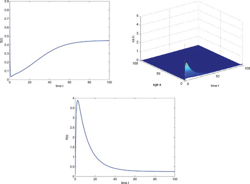
We adopt the following values for the parameters motivated by bovine TB in a cattle herd with time unit of one year [25]: $A=\mu =0.1,\delta =0.5,\gamma \left(a\right)=0.5$.

The transmission coefficient of the infected individuals at age of infection a is chosen as (94) $\beta \left(a\right)=\left\{\begin{array}{ll}0,& a<0.75,\\ 0.6,& a\ge \mathrm{0.75.}\end{array}\right.$(94) By calculation, we obtain the basic reproduction number ${\mathcal{R}}_0=\mathrm{1.3319.}$ By Theorem 4.1, we see that in addition to the infection-free steady state $E_1(1,0,0)$, system (2(2) $\begin{array}{rl}& \dot{S}\left(t\right)=A-\mu S\left(t\right)-S\left(t\right){\int }_0^{\mathrm{\infty }}\beta \left(a\right)i(a,t)\mathrm{d}a,\\ & \frac{\mathrm{\partial }i(a,t)}{\mathrm{\partial }t}+\frac{\mathrm{\partial }i(a,t)}{\mathrm{\partial }a}=-(\mu +\gamma (a\left)\right)i(a,t),a>0,\\ & \dot{R}\left(t\right)={\int }_0^{\mathrm{\infty }}\gamma \left(a\right)i(a,t)\mathrm{d}a-(\mu +\delta )R\left(t\right),\end{array}$(2) ) has an endemic steady state $E^{\ast }(0.4810,0.1687{\mathrm{e}}^{-0.6a},0.1384)$ which is locally asymptotically stable. Numerical simulation illustrates this fact (see Figure 1).

Figure 1. The temporal solution found by numerical integration of system (2(2) $\begin{array}{rl}& \dot{S}\left(t\right)=A-\mu S\left(t\right)-S\left(t\right){\int }_0^{\mathrm{\infty }}\beta \left(a\right)i(a,t)\mathrm{d}a,\\ & \frac{\mathrm{\partial }i(a,t)}{\mathrm{\partial }t}+\frac{\mathrm{\partial }i(a,t)}{\mathrm{\partial }a}=-(\mu +\gamma (a\left)\right)i(a,t),a>0,\\ & \dot{R}\left(t\right)={\int }_0^{\mathrm{\infty }}\gamma \left(a\right)i(a,t)\mathrm{d}a-(\mu +\delta )R\left(t\right),\end{array}$(2) ) with the boundary condition (3(3) $i(0,t)=S\left(t\right){\int }_0^{\mathrm{\infty }}\beta \left(a\right)i(a,t)\mathrm{d}a+\delta R\left(t\right),$(3) ) and the initial condition $S\left(0\right)=0.9,i(\cdot ,0)=0.1,R\left(0\right)=0$.

8. Discussion

In this work, a PDE infectious disease model was proposed to incorporate disease relapse and the infection age of infectious individuals. It has been shown that the global dynamics of system (2(2) $\begin{array}{rl}& \dot{S}\left(t\right)=A-\mu S\left(t\right)-S\left(t\right){\int }_0^{\mathrm{\infty }}\beta \left(a\right)i(a,t)\mathrm{d}a,\\ & \frac{\mathrm{\partial }i(a,t)}{\mathrm{\partial }t}+\frac{\mathrm{\partial }i(a,t)}{\mathrm{\partial }a}=-(\mu +\gamma (a\left)\right)i(a,t),a>0,\\ & \dot{R}\left(t\right)={\int }_0^{\mathrm{\infty }}\gamma \left(a\right)i(a,t)\mathrm{d}a-(\mu +\delta )R\left(t\right),\end{array}$(2) ) is determined completely by the basic reproduction number ${\mathcal{R}}_0$. By constructing suitable Lyapunov functionals and using LaSalle's invariance principle, it has been shown that if the basic reproduction number is less than unity, the disease-free steady state is globally asymptotically stable and the disease dies out; if the basic reproduction number is greater than unity, the endemic steady state is globally asymptotically stable and the disease persists. The global stability of the endemic steady state rules out any possibility for the existence of Hopf bifurcations and sustained oscillations in system (2(2) $\begin{array}{rl}& \dot{S}\left(t\right)=A-\mu S\left(t\right)-S\left(t\right){\int }_0^{\mathrm{\infty }}\beta \left(a\right)i(a,t)\mathrm{d}a,\\ & \frac{\mathrm{\partial }i(a,t)}{\mathrm{\partial }t}+\frac{\mathrm{\partial }i(a,t)}{\mathrm{\partial }a}=-(\mu +\gamma (a\left)\right)i(a,t),a>0,\\ & \dot{R}\left(t\right)={\int }_0^{\mathrm{\infty }}\gamma \left(a\right)i(a,t)\mathrm{d}a-(\mu +\delta )R\left(t\right),\end{array}$(2) ). A similar dynamic behavior has been observed in [31].

Solving the second equation of system (2(2) $\begin{array}{rl}& \dot{S}\left(t\right)=A-\mu S\left(t\right)-S\left(t\right){\int }_0^{\mathrm{\infty }}\beta \left(a\right)i(a,t)\mathrm{d}a,\\ & \frac{\mathrm{\partial }i(a,t)}{\mathrm{\partial }t}+\frac{\mathrm{\partial }i(a,t)}{\mathrm{\partial }a}=-(\mu +\gamma (a\left)\right)i(a,t),a>0,\\ & \dot{R}\left(t\right)={\int }_0^{\mathrm{\infty }}\gamma \left(a\right)i(a,t)\mathrm{d}a-(\mu +\delta )R\left(t\right),\end{array}$(2) ) with the boundary condition (3(3) $i(0,t)=S\left(t\right){\int }_0^{\mathrm{\infty }}\beta \left(a\right)i(a,t)\mathrm{d}a+\delta R\left(t\right),$(3) ) and the initial condition (4(4) $X_0:=\left(S\left(0\right),i(\cdot ,0),R\left(0\right)\right)=\left(S^0,i_0(\cdot ),R^0\right)\in \mathcal{X},$(4) ), one has (95) $i(a,t)=\left\{\begin{array}{ll}i(0,t-a){\mathrm{e}}^{-{\int }_0^a(\mu +\gamma (s\left)\mathrm{d}s\right)},& 0\le a\le t,\\ i_0(a-t){\mathrm{e}}^{-{\int }_{a-t}^a(\mu +\gamma (s\left)\right)\mathrm{d}s},& 0\le t\le a.\end{array}\right.$(95) We further assume in Equation (2(2) $\begin{array}{rl}& \dot{S}\left(t\right)=A-\mu S\left(t\right)-S\left(t\right){\int }_0^{\mathrm{\infty }}\beta \left(a\right)i(a,t)\mathrm{d}a,\\ & \frac{\mathrm{\partial }i(a,t)}{\mathrm{\partial }t}+\frac{\mathrm{\partial }i(a,t)}{\mathrm{\partial }a}=-(\mu +\gamma (a\left)\right)i(a,t),a>0,\\ & \dot{R}\left(t\right)={\int }_0^{\mathrm{\infty }}\gamma \left(a\right)i(a,t)\mathrm{d}a-(\mu +\delta )R\left(t\right),\end{array}$(2) ) that $\beta \left(a\right)={\beta }_1,\gamma \left(a\right)={\gamma }_1$.

When t is sufficiently large (being greater than all possible infection ages), we have (96) $i(a,t)=i(0,t-a){\mathrm{e}}^{-{\int }_0^a(\mu +\gamma (s\left)\right)\mathrm{d}s}=i(0,t-a){\mathrm{e}}^{-(\mu +{\gamma }_1)a}.$(96) Denote (97) $I\left(t\right)={\int }_0^{\mathrm{\infty }}i(a,t)\mathrm{d}a.$(97) Noting that $\mathrm{\partial }i(a,t)/\mathrm{\partial }t=-(\mu +{\gamma }_1)i(a,t)-\mathrm{\partial }i(a,t)/\mathrm{\partial }a$, we obtain from Equation (97(97) $I\left(t\right)={\int }_0^{\mathrm{\infty }}i(a,t)\mathrm{d}a.$(97) ) that (98) $\begin{array}{rl}\frac{\mathrm{d}}{\mathrm{d}t}I\left(t\right)& ={\int }_0^{\mathrm{\infty }}\frac{\mathrm{\partial }}{\mathrm{\partial }t}i(a,t)\mathrm{d}a\\ & =-{\int }_0^{\mathrm{\infty }}\left(\frac{\mathrm{\partial }i(a,t)}{\mathrm{\partial }a}+(\mu +{\gamma }_1)i(a,t)\right)\mathrm{d}a\\ & =-i(a,t){|}_0^{\mathrm{\infty }}-(\mu +{\gamma }_1){\int }_0^{\mathrm{\infty }}i(a,t)\mathrm{d}a.\end{array}$(98) It follows from Equation (96(96) $i(a,t)=i(0,t-a){\mathrm{e}}^{-{\int }_0^a(\mu +\gamma (s\left)\right)\mathrm{d}s}=i(0,t-a){\mathrm{e}}^{-(\mu +{\gamma }_1)a}.$(96) ) that (99) $\begin{array}{rl}\underset{a\to +\mathrm{\infty }}{lim}i(a,t)& =\underset{a\to +\mathrm{\infty }}{lim}i(0,t-a){\mathrm{e}}^{-(\mu +{\gamma }_1)a}\\ & =\underset{a\to +\mathrm{\infty }}{lim}{\mathrm{e}}^{-(\mu +{\gamma }_1)a}\left({\beta }_{1}S(t-a){\int }_0^{\mathrm{\infty }}i(a,t-a)\mathrm{d}a+\delta R(t-a)\right)\\ & =0.\end{array}$(99) We therefore derive from Equations (3(3) $i(0,t)=S\left(t\right){\int }_0^{\mathrm{\infty }}\beta \left(a\right)i(a,t)\mathrm{d}a+\delta R\left(t\right),$(3) ) and (98(98) $\begin{array}{rl}\frac{\mathrm{d}}{\mathrm{d}t}I\left(t\right)& ={\int }_0^{\mathrm{\infty }}\frac{\mathrm{\partial }}{\mathrm{\partial }t}i(a,t)\mathrm{d}a\\ & =-{\int }_0^{\mathrm{\infty }}\left(\frac{\mathrm{\partial }i(a,t)}{\mathrm{\partial }a}+(\mu +{\gamma }_1)i(a,t)\right)\mathrm{d}a\\ & =-i(a,t){|}_0^{\mathrm{\infty }}-(\mu +{\gamma }_1){\int }_0^{\mathrm{\infty }}i(a,t)\mathrm{d}a.\end{array}$(98) )–(99(99) $\begin{array}{rl}\underset{a\to +\mathrm{\infty }}{lim}i(a,t)& =\underset{a\to +\mathrm{\infty }}{lim}i(0,t-a){\mathrm{e}}^{-(\mu +{\gamma }_1)a}\\ & =\underset{a\to +\mathrm{\infty }}{lim}{\mathrm{e}}^{-(\mu +{\gamma }_1)a}\left({\beta }_{1}S(t-a){\int }_0^{\mathrm{\infty }}i(a,t-a)\mathrm{d}a+\delta R(t-a)\right)\\ & =0.\end{array}$(99) ) that (100) $\begin{array}{rl}\frac{\mathrm{d}}{\mathrm{d}t}I\left(t\right)& ={\beta }_{1}S\left(t\right){\int }_0^{\mathrm{\infty }}i(a,t)\mathrm{d}a+\delta R\left(t\right)-(\mu +{\gamma }_1)I\left(t\right)\\ & ={\beta }_{1}S\left(t\right)I\left(t\right)+\delta R\left(t\right)-(\mu +{\gamma }_1)I\left(t\right).\end{array}$(100) Hence, if $\beta \left(a\right)$ and $\gamma \left(a\right)$ are constants, then system (2(2) $\begin{array}{rl}& \dot{S}\left(t\right)=A-\mu S\left(t\right)-S\left(t\right){\int }_0^{\mathrm{\infty }}\beta \left(a\right)i(a,t)\mathrm{d}a,\\ & \frac{\mathrm{\partial }i(a,t)}{\mathrm{\partial }t}+\frac{\mathrm{\partial }i(a,t)}{\mathrm{\partial }a}=-(\mu +\gamma (a\left)\right)i(a,t),a>0,\\ & \dot{R}\left(t\right)={\int }_0^{\mathrm{\infty }}\gamma \left(a\right)i(a,t)\mathrm{d}a-(\mu +\delta )R\left(t\right),\end{array}$(2) ) reduces to system (1(1) $\begin{array}{rl}\dot{S}\left(t\right)& =A-\mu S\left(t\right)-\beta S\left(t\right)I\left(t\right),\\ \dot{I}\left(t\right)& =\beta S\left(t\right)I\left(t\right)-(\mu +\gamma )I\left(t\right)+\delta R\left(t\right),\\ \dot{R}\left(t\right)& =\gamma I\left(t\right)-(\mu +\delta )R\left(t\right).\end{array}$(1) ).

By choosing appropriate kernel functions, system (2(2) $\begin{array}{rl}& \dot{S}\left(t\right)=A-\mu S\left(t\right)-S\left(t\right){\int }_0^{\mathrm{\infty }}\beta \left(a\right)i(a,t)\mathrm{d}a,\\ & \frac{\mathrm{\partial }i(a,t)}{\mathrm{\partial }t}+\frac{\mathrm{\partial }i(a,t)}{\mathrm{\partial }a}=-(\mu +\gamma (a\left)\right)i(a,t),a>0,\\ & \dot{R}\left(t\right)={\int }_0^{\mathrm{\infty }}\gamma \left(a\right)i(a,t)\mathrm{d}a-(\mu +\delta )R\left(t\right),\end{array}$(2) ) also contains infectious disease models with time delay, and the global stability result in this work provides the global dynamics for these delayed epidemic models.

Acknowledgments

The author wishes to thank the Editor and the reviewers for their valuable comments and suggestions that greatly improved the presentation of this work.

Disclosure statement

No potential conflict of interest was reported by the author.

Additional information

Funding

This work was supported by the National Natural Science Foundation of China under grant 11371368 and the Natural Science Foundation of Hebei Province under grant A2014506015.

References

- A. Bernoussi, A. Kaddar, and S. Asserda, Global stability of a delayed SIRI epidemic model with nonlinear incidence, Int. J. Eng. Math. 2014 (2014), pp. 1–6. Article ID 487589. doi: 10.1155/2014/487589
- S.M. Blower, T.C. Porco, and G. Darby, Predicting and preventing the emergence of antiviral drug resistance in HSV-2, Nat. Med. 4(6) (1998), pp. 673–678. doi: 10.1038/nm0698-673
- F. Brauer, Z. Shuai, and P. van den Driessche, Dynamics of an age-of-infection cholera model, Math. Biosci. Eng. 10(5–6) (2013), pp. 1335–1349.
- Y. Chen, J. Yang, and F. Zhang, The global stability of an SIRS model with infection age, Math. Biosci. Eng. 11(3) (2014), pp. 449–469. doi: 10.3934/mbe.2014.11.449
- J. Chin, Control of Communicable Diseases Manual, American Public Health Association, Washington, DC, 1999.
- E.L. Corbett, C.J. Watt, N. Walker, D. Maher, B. Williams, M. Raviglione, and C. Dye, The growing burden of tuberculosis: Global trends and interactions with the HIV epidemic, Arch. Intern. Med. 163(9) (2003), pp. 1009–1021. doi: 10.1001/archinte.163.9.1009
- X. Duan, S. Yuan, and X. Li, Global stability of an SVIR model with age of vaccination, Appl. Math. Comput. 226 (2014), pp. 528–540.
- X. Duan, S. Yuan, Z. Qiu, and J. Ma, Global stability of an SVEIR epidemic model with ages of vaccination and latency, Comput. Math. Appl. 68(3) (2014), pp. 288–308. doi: 10.1016/j.camwa.2014.06.002
- A. Ducrot and P. Magal, Travelling wave solutions for an infection-age structured epidemic model with external supplies, Nonlinearity 24(10) (2011), pp. 2891–2911. doi: 10.1088/0951-7715/24/10/012
- Z. Feng, M. Iannelli, and F.A. Milner, A two-strain tuberculosis model with age of infection, SIAM. J. Appl. Math. 62(5) (2002), pp. 1634–1656. doi: 10.1137/S003613990038205X
- P. Georgescu and H. Zhang, A Lyapunov functional for a SIRI model with nonlinear incidence of infection and relapse, Appl. Math. Comput. 219(16) (2013), pp. 8496–8507.
- H. Guo, M.Y. Li, and Z. Shuai, Global dynamics of a general class of multistage models for infectious diseases, SIAM J. Appl. Math. 72(1) (2012), pp. 261–279. doi: 10.1137/110827028
- J.K. Hale and P. Waltman, Persistence in infinite dimensional systems, SIAM J. Math. Anal. 20(2) (1989), pp. 388–395. doi: 10.1137/0520025
- T. Hart, Microterrors, Firefly Books, New York, 2004.
- M. Iannelli, Mathematical Theory of Age-Structured Population Dynamics, Applied Mathematics Monographs, Vol. 7, comitato nazionale per le scienze matematiche, Consiglio Nazionale delle Ricerche (C.N.R), Giardini, Pisa, 1995.
- S.D. Lawn, R. Wood, and R.J. Wilkinson, Changing concepts of ‘latent tuberculosis infection’ in patients living with HIV infection, Clin. Dev. Immunol. 2011 (2011), pp. 1–9. Article ID 980594. doi: 10.1155/2011/980594
- P. Magal, Compact attractors for time periodic age-structured population models, Electron. J. Differ. Equ. 2001(65) (2001), pp. 1–35.
- P. Magal, C.C. McCluskey, and G.F. Webb, Lyapunov functional and global asymptotic stability for an infection-age model, Appl. Anal. 89(7) (2010), pp. 1109–1140. doi: 10.1080/00036810903208122
- S.W. Martin, Livestock Disease Eradication: Evaluation of the Cooperative State-Federal Bovine Tuberculosis Eradication Program, National Academy Press, Washington, DC, 1994.
- H.N. Moreira and Y. Wang, Classroom note: Global stability in a S → I → R → I model, SIAM Rev. 39(3) (1997), pp. 496–502. doi: 10.1137/S0036144595295879
- H.L. Smith and H.R. Thieme, Dynamical Systems and Population Persistence, American Mathematical Society, Providence, 2011.
- D. Tudor, A deterministic model for herpes infections in human and animal populations, SIAM Rev. 32(1) (1990), pp. 136–139. doi: 10.1137/1032003
- P. van den Driessche and J. Watmough, Reproduction numbers and sub-threshold endemic equilibria for compartmental models of disease transmission, Math. Biosci. 180(1–2) (2002), pp. 29–48. doi: 10.1016/S0025-5564(02)00108-6
- P. van den Driessche and X. Zou, Modeling relapse in infectious diseases, Math. Biosci. 207(1) (2007), pp. 89–103. doi: 10.1016/j.mbs.2006.09.017
- P. van den Driessche, L. Wang, and X. Zou, Modeling diseases with latency and relapse, Math. Biosci. Eng. 4(2) (2007), pp. 205–219. doi: 10.3934/mbe.2007.4.205
- K.E. VanLandingham, H.B. Marsteller, G.W. Ross, and F.G. Hayden, Relapse of herpes simplex encephalitis after conventional acyclovir therapy, J. Am. Med. Assoc. 259(7) (1988), pp. 1051–1053. doi: 10.1001/jama.1988.03720070051034
- C. Vargas-De-Leon, On the global stability of infectious diseases models with relapse, Abstr. Appl. 9 (2013), pp. 50–61.
- J. Wang, J. Zu, X. Liu, G. Huang, and J. Zhang, Global dynamics of a multi-group epidemic model with general relapse distribution and nonlinear incidence rate, J. Biol. Syst. 20(3) (2012), pp. 235–258. doi: 10.1142/S021833901250009X
- G. Webb, Theory of Nonlinear Age-Dependent Population Dynamics, Marcel Dekker, New York, 1985.
- R. Xu, Global dynamics of a delayed epidemic model with latency and relapse, Nonlinear Anal. Model. Control 18(2) (2013), pp. 250–263. doi: 10.15388/NA.18.2.14026
- R. Xu, X. Tian and S. Zhang, An age-structured within host HIV-1 infection model with virus-to-cell and cell-to-cell transmissions, J. Biol. Dyn., 12(1)(2018), pp. 89–117. doi: 10.1080/17513758.2017.1404646
- J.-Y. Yang, X.-Z. Li, and M. Martcheva, Global stability of a DS-DI epidemic model with age of infection, J. Math. Anal. Appl. 385(2) (2012), pp. 655–671. doi: 10.1016/j.jmaa.2011.06.087
- J. Yang, Z. Qiu, and X .-Z. Li, Global stability of an age-structured cholera model, Math. Biosci. Eng. 11(3) (2014), pp. 641–665. doi: 10.3934/mbe.2014.11.641