Singular stochastic control model for algae growth management in dam downstream

ABSTRACT

A stochastic control model for finding an ecologically sound, fit-for-purpose dam operation policy to suppress bloom of attached algae in its downstream is presented. A singular exactly solvable and a more realistic regular-singular cases are analysed in terms of a Hamilton–Jacobi–Bellman equation. Regularity and consistency of the value function are analysed and its classical verification theorem is established. Practical implications of the mathematical analysis results are discussed focusing on parameter dependence of the optimal controls. An asymptotic analysis with a numerical computation reveals solution behaviour of the Hamilton–Jacobi–Bellman equation near the origin, namely at the early stage of algae growth.

KEYWORDS:

• Stochastic differential equation
• singular control
• regular-singular control
• attached algae
• Hamilton–Jacobi–Bellman equation

CLASSIFICATION CODES:

• 49L20
• 62P12
• 93E20

1. Introduction

Dam is a water infrastructure indispensable for life of modern people [46]. River discharge downstream of a dam is strongly regulated by its outflow, which often deviates from the natural ones in both quantity and quality [19,49]. Lowering the magnitude and fluctuations of river discharge is a common environmental issue that a river equipped with a dam encounters, which often results in severe degradation of the downstream river environment and ecosystems [9,35,43]. One of the most severe issues among them is the bloom of harmful attached algae, such as periphyton, on the riverbed in dam downstream [6,31,32]. The harmful attached algae, hereafter simply referred to as the algae for the sake of simplicity of descriptions, have been reported to provide a variety of disutilities. Such examples include qualitative changes of food webs directly and indirectly as the producer in aquatic ecosystems [18,23,36], degradation of river landscape [39], nasty smell from dead algae [29,58], and degradation of the quality of inland fishery resources [24]. Establishment of ecologically sound as well as fit-for-purpose operation policies of dams to suppress the algae bloom is currently an urgent environmental issue worldwide.

It has been found by the experimental and field investigations that the algae are gradually detached from the riverbed by the bedload transport and shear stresses [7,13], indicating that river discharge should not be too small to suppress their growth. Deterministic and mechanistic population dynamics models have been applied to simulating the algae detachment processes [7,16,17,34,51]. In reality, biological dynamics like the population dynamics of algae is essentially stochastic, and application of a stochastic process model is more appropriate for its analysis [1,61]. Recently, the authors applied a stochastic process model for evaluation of the algae growth in a Japanese river environment, demonstrating reasonable agreement between the predicted and observed algae population dynamics [58]. However, most of the above-mentioned researchers keep heuristic discussion and analyse the problem from engineering viewpoint rather than mathematical one. Analysis of the algae growth from a mathematical viewpoint would provide better comprehension of the dynamics and effective ways to manage them. This is a strong motivation of this paper.

The objective of this paper is formulation and analysis of a stochastic control model for finding the ecologically sound as well as fit-for purpose management policy of the attached algae downstream of a dam: an urgent environmental and ecological issue. We employ a stochastic differential equation (SDE) for describing the algae population dynamics. The SDE has two contrasting control variables; one of them is the dam discharge that is regular, while the other is singular that turns out to give the threshold to suppress the algae growth. Stochastic control problems based on SDEs have been central mathematical topics in wide range of research fields. Such examples include economics [28,47], finance and insurance [25,50,63], environmental science [10,27], and ecology [61,52,54]. Regular-singular stochastic control problems with analytical solutions have been mathematically analysed for economic problems [11,21,62]. For management of algae growth, it is reasonable to set the upper threshold of its population (or population density), above which the aquatic environment and ecosystems are severely affected [36]. This management policy would be effectively analysed within the context of the singular control. To our knowledge, no attempt has been made for singular control modelling of the algae growth and their management despite its potential applicability to the problem. Regular-singular stochastic control modelling of the algae growth is therefore a new attempt, which would give new insights on the management problem from both mathematical and practical viewpoints.

The singular control of the present SDE is slightly different from the conventional ones [3, Chapter 4.5 of 44] in that the singular control variable is multiplied by a power function of the state variable in the former. Related SDEs with a not usual but simpler singular control terms multiplied by state variables have been mathematically and numerically analysed [2,22,38,41,48]. A performance index to be maximized by the decision-maker, which is the manager of the dam, is presented under the assumptions that there exists a target value of the dam discharge and that the growth of algae is considered as not desirable. The stochastic control problem effectively reduces to a boundary value problem of a Hamilton–Jacobi–Bellman (HJB) equation: a degenerate elliptic variational inequality. A series of regularity results on the value function, the maximized performance index, are derived. In addition, the value function is characterized as a locally Lipschitz continuous viscosity solution to the HJB equation [44,15]. An explicit exact solution as the unique classical as well as viscosity solution to the HJB equation with the uncontrolled dam discharge is derived and its practical implications are presented. A more realistic regular-singular case with the controlled dam discharge is also analysed with the help of an asymptotic analysis technique, which clearly shows dependence of the optimal dam discharge on the early stage of algae growth. Numerical computation of the HJB equation is also carried out to validate the mathematical analysis results. The present mathematical model thus forms a regular-singular stochastic control problem having a sound application.

The rest of this paper is organized as follows. Section 2 formulates the problem and derives the HJB equation. Section 3 analyses regularity, parameter dependence, and viscosity property of the value function. Section 4 analyses the HJB equation with the uncontrolled dam discharge. Section 4 also deals with the problem with the controlled dam discharge and presents its numerical solutions that validate the mathematical analysis results. Section 5 concludes this paper and presents future perspectives of our research.

2. Mathematical model

2.1. Problem setting

Population dynamics of attached algae on riverbed just downstream of a dam is considered. The main assumption made in the present mathematical model is that the detachment process of the algae is due to the physical factors by the bedload transport and shear stress [51]. In addition, it is assumed that the algae growth can be suppressed by the decision-maker, the manager of the dam, through activities such as river cleaning. The SDE here is based on a geometric Brownian type, which is a linearized counterpart of the logistic type models [20] employed in the algae population dynamics models [58]. Employing the simpler SDE allows us to derive a tractable model as demonstrated later.

The time is denoted as $t\ge 0$. The 1-D standard Brownian motion on the complete probability space is denoted as $B_t$. The population of the algae on the riverbed, such as the unit-area biomass, at the time $t$ is considered as a non-negative stochastic process $X_t$. There are two control variables in the present model. The one is the dam discharge $q_t$, which is bounded, measurable, and has the compact range $Q=\left[q_{min},q_{max}\right]$, $0\le q_{min}\le q_{max}$. The other is the non-decreasing right-continuous process ${\eta }_t$ having left-side limit [44], which turns out to give the allowable threshold of the algae growth, above which the aquatic environment and ecosystems are severely affected. The control ${\eta }_t$ conceptually represents a decrease in the algae population rather than by controlling the dam discharge $q_t$. A typical and actually performed example in Japan is cleaning up of the riverbed by residents and/or local governments. Another example is controlling water quality and water environment surrounding the algae, such as improvement of water quality in the water stored in the dam so that the algae growth is suppressed. These countermeasures possibly lead to rapid environmental changes with time scales significantly smaller than that of the algae growth, thus can be represented as a singular control variable. Both control variables are adapted to a natural filtration generated by $B_t$. The controls $q_t$ and ${\eta }_t$ are chosen so that the SDE (1) has a unique strong solution such that $X_t\ge 0$, $t\ge 0$. The set of admissible controls $q_t$ and ${\eta }_t$ complying with the above-mentioned requirements are expressed as ${\theta }_q$ and ${\theta }_{\eta }$, respectively. The subscript of the control variables is often omitted when there is no confusion.

2.2. Controlled SDEs

Hereafter, the notation $X_{t-}=X_{t-0}$ is employed for the sake of brevity of descriptions. The Itô’s SDE that governs $X_t$ ($t\ge 0$) with the initial condition $X_{-0}=x\ge 0$ is set as (1) $\text{d}{X}_t=(r-R(q_t\left)\right)X_{t-}\text{d}t+\sigma X_{t-}\text{d}{B}_t-X_{t-}^l\text{d}{\eta }_t,R\left(q_t\right)=\frac{k{q}_t^{1+n}}{1+n},$(1) where $r>0$ is the deterministic growth rate of the algae, $\sigma >0$ is the parameter that modulates inherent stochastic fluctuations involved in the population dynamics, $R=R\left(q_t\right)$ is the detachment rate of the algae as a power function of the dam discharge $q_t$, $k>0$, $n>-1$, and $0\le l\le 1$ are the constant parameters to represent detachment characteristics of the algae. The parameter $\sigma$ involves fluctuations of the dam discharge that cannot be resolved in the first term of the SDE (1). Notice that the set $\theta =\left\{(q,\eta );q\in {\theta }_q,\eta \in {\theta }_{\eta }\right\}$ is not empty. This is because at least $q_t=const\in \left[q_{min},q_{max}\right]$ and ${\eta }_t\equiv 0$ are admissible.

The parameters $k$ and $n$ represent the magnitude of the detachment rate and its sensitivity on the discharge $q_t$. The value of the parameter $n$ may depend on the algae species. Fovet et al. [16,17] imply that $n=0$ is appropriate for some periphyton. On the other hand, for the macroalgae Cladophora glomerata Kützing, the previous research implies $R\left(q\right)=O\left(W\right)$ [58,51]. Here, $W$ is the work rate done by saltation of gravel bed materials that satisfies $W=O\left(q_{\mathrm{B}}{\tau }^{1/3}\right)$ where the bed shear stress is denoted as $\tau$ and the bedload discharge as $q_{\mathrm{B}}$. The empirical Manning’s formula for bed shear stress gives $\tau =O\left(q^{6/10}\right)$ [5] and the Meyer-Peter and Müller’s formula for bedload transport [37] gives $q_{\mathrm{B}}=O\left({\tau }^{3/2}\right)$. Summarizing the above results yields $W=O\left({\tau }^{11/6}\right)$ and hence $R\left(q\right)=O\left(q^{11/10}\right)$ with $n=1/10$. However, since these relationships are estimated from the empirical formulae, our model assumes $n>-1$, so that wider range of problems are handled. The parameter $l$ represents the effectiveness of the singular control term $X_t^l\text{d}{\eta }_t$ (understood in the sense like [2]), the decrease in the algae population rather than by controlling the discharge. This parameter would depend on the algae species, and on the method to suppress the algae growth. The possible range of the parameter $l$ is specified so that the problem with a conventional singular term ($l=0$), proportional singular term ($l=1$), and the intermediate case ($0<l<1$) is covered. This parameter would depend on the algae species, and on the method to suppress the algae growth. This is a practical rather than mathematical problem, and is not focused on in this paper.

Remark 2.1

The process ${\eta }_t$ ($t\ge 0$) admits the cumulative representation [14] (2) ${\eta }_t={\int }_0^t{a}_s\text{d}s(\text{or}\text{equivalently}\text{d}{\eta }_t=a_t\text{d}t),$(2) with an unbounded non-negative process $a_t$ ($t\ge 0$).

2.3. Performance index

The performance index to be maximized by the decision-maker is formulated from dam operational and ecological viewpoints. The performance index is denoted as $J=J(x;q,\eta )$ and is formulated as (3) $J=E^x\left[J_1+J_2+J_3\right],$(3) where $E^x$ is the conditional expectation with $X_{-0}=x\ge 0$. Each $J_i$ ($i=1,2,3$) is specified as follows. Firstly, $J_1$ measures the deviation between the current dam discharge $q$ and its target value $\overline{q}$ ($q_{min}\le \overline{q}\le q_{max}$) prescribed based on the purpose of the dam, which is assumed to be a positive constant, as (4) $J_1=-{\int }_0^{\tau }{e}^{-\delta s}\frac{1}{2p}{\left(q_s-\overline{q}\right)}^{2p}\text{d}s,$(4) where $\tau \ge 0$ is the first-hitting time of $X_{\tau }=0$, $p>(n+1)/2$ is a natural number, and $\delta >0$ is the discount factor. The parameter $p$ represents the sensitivity of the decision-maker on the deviation $|q_s-\overline{q}|$. In the present model, $\delta$ represents the attitude of the manager of the dam; larger $\delta$ means that the manager addresses the problem from a longer term viewpoint, and vice versa. Secondly, $J_2$ measures ecological, environmental, fisheries, and social disutilities that the algae provide in a lumped manner as (5) $J_2=-{\int }_0^{\tau }{e}^{-\delta s}\frac{\gamma }{m+1}{X}_s^{m+1}\text{d}s,$(5) where $\gamma >0$ is the weight constant and $-l<m\le 1$ is the sensitivity of the disutility on the algae population. Finally, $J_3$ measures the cost to suppress the algae growth as (6) $J_3=-{\int }_0^{\tau }\beta e^{-\delta s}\text{d}{\eta }_s,$(6) where $\beta >0$ is the weight constant. The performance index in Equation (3) is different from the conventional one [58] in that the term $J_3$ exists and $p=1$ in the latter. The assumptions $p>(n+1)/2$ and $-l<m\le 1$ on the parameters are employed for technical reasons to facilitate the mathematical analysis in this paper. The condition $p>(n+1)/2$ means that the decision-maker is sufficiently sensitive to the deviation $|q_t-\overline{q}|$. The condition $-l<m\le 1$ means that the decision-maker is sufficiently sensitive to the algae growth.

Remark 2.2

By Remark 2.1, $J_3$ is expressed with $a$ as (7) $J_3=-{\int }_0^{\tau }\beta e^{-\delta s}{a}_s\text{d}s.$(7)

The performance index maximized with respect to admissible $q$ and $\eta$ is defined as the value function $\mathrm{\Phi }=\mathrm{\Phi }\left(x\right)$: (8) $\mathrm{\Phi }=\underset{q\in {\theta }_q,\eta \in {\theta }_{\eta }}{sup}J.$(8) The value function $\mathrm{\Phi }$ can be interpreted as the minimized net management cost. The optimal $q$ and $\eta$ to archive the maximization are expressed as $q^{\ast }$ and ${\eta }^{\ast }$, and are referred to as the optimal (Markov) controls. The discount factor $\delta >0$ is assumed to be sufficiently large, so that $\mathrm{\Phi }$ is locally bounded. For this purpose, the following assumption is made throughout this paper.

Assumption 2.1

(9) $E=\delta -(m+1)(r-R(\overline{q}\left)\right)-\frac{1}{2}m(m+1){\sigma }^2>0.$(9) This means that the decision-maker is sufficiently patient since $\delta$ represents the patience of the decision-maker. Assumption 2.1 is sufficient to guarantee the local boundedness of $\mathrm{\Phi }$ as shown in Proposition 3.1.

2.3. Hamilton–Jacobi–Bellman equation

The HJB equation is a variational inequality that governs $\mathrm{\Phi }=\mathrm{\Phi }\left(x\right)$. Applying the dynamic programming principle as in some of the literatures ([2], Chapter 2.2 of [4], [23], [39]), the HJB equation is formally derived as (10) $min\left\{-\underset{q\in Q}{max}{L}_q\mathrm{\Phi },x^l\frac{\text{d}\mathrm{\Phi }}{\text{d}x}+\beta \right\}=0,x>0,$(10) where $L_q$ is the operator defined for generic sufficiently smooth $f=f\left(x\right)$ as (11) $L_{q}f=-\delta f+\frac{{\sigma }^2{x}^2}{2}\frac{{\text{d}}^{2}f}{\text{d}{x}^2}+\left(r-\frac{k{q}^{1+n}}{1+n}\right)x\frac{\text{d}f}{\text{d}x}-\frac{\gamma }{1+m}{x}^{m+1}-\frac{1}{2p}(q-\overline{q}{)}^{2p}.$(11)

At each $x>0$, the maximizer of the term $\underset{q\in Q}{max}{L}_q\mathrm{\Phi }$ can be seen as a function of $x$. This maximizer is then expressed as $q^{\ast }=q^{\ast }\left(x\right)$ with the abuse of notation since the optimal dam discharge at each time $t$ is expressed as $q^{\ast }=q^{\ast }\left(X_t\right)$. The HJB equation is subject to the boundary condition $|\mathrm{\Phi }\left(0\right)|<+\mathrm{\infty }$, which turns out to be $\mathrm{\Phi }\left(0\right)=0$ later.

Remark 2.3

By Remarks 2.1 and 2.2, Equation (10) can be rewritten as (12) $-\underset{q\in Q,a\ge 0}{max}{L}_{q,a}\mathrm{\Phi }=0,x>0,$(12) where $L_{q,a}$ is the operator defined for generic sufficiently smooth $f=f\left(x\right)$ as (13) $\begin{array}{rl}{L}_{q,a}f& =-\delta f+\frac{{\sigma }^2{x}^2}{2}\frac{{\text{d}}^{2}f}{\text{d}{x}^2}+\left(r-\frac{k{q}^{1+n}}{1+n}\right)x\frac{\text{d}f}{\text{d}x}-\frac{\gamma }{1+m}{x}^{m+1}-\frac{1}{2p}(q-\overline{q}{)}^{2p}\\ & -a\left(x^l\frac{\text{d}f}{\text{d}x}+\beta \right).\end{array}$(13) Formally, the left-hand side of Equation (12) is unbounded if $x^l\frac{\text{d}\mathrm{\Phi }}{\text{d}x}+\beta <0$ with the optimal $a^{\ast }=+\mathrm{\infty }$, which turns to be false for viscosity solutions as shown in the next section.

Remark 2.4

It may be more natural to consider $-J$ as the cost. Nevertheless, this paper adopts the non-positive cost as in the previous papers [58,60], so that a cost is consistently considered as a non-positive value. It should be noted that to consider the cost as a non-positive value or a non-negative value does not affect the mathematical analysis results of this paper.

2.4. Discussion on the model assumptions

This paper is on theory and mathematical analysis of the controlled algae population dynamics. The present mathematical model is based on a series of assumptions, which should be justified. This sub-section summarizes these assumptions and discusses when they can be justified.

The present mathematical model consists of the two mathematical concepts: the SDE (1) and the performance index (Equation (3)). For each $q_t\in {\theta }_q$, the SDE (1) without the third term is a minimal SDE that describes temporal evolution of a non-negative quantity, such as a population. The coefficients involved in these terms are based on physical and biological considerations [58,16,17,51]. The third term represents the decrease in the algae population rather than by controlling the discharge $q_t$, which is a very flexible term by the existence of the coefficient $X_t^l$. This term can potentially represent the direct ($l=0$, such as cleaning up the river by residents and/or local governments) and indirect decrease in the population ($l=1$, such as controlling the growth rate of the algae population by modifying its surrounding water environment) in particular. This term can potentially handle even the intermediate case $\left(0<l<1\right)$ that can be seen as a direct (indirect) decrease case in which its effectiveness increases (decreases) as the population $X_t$ decreases (increases). Although the SDE (1) seems to be simple, it has a flexibility to handle a variety of cases. The model parameters can be identified through physical and biological experiments. More realistic problems where the growth rate depends on the population $X_t$ like the conventional logistic models can be handled at least numerically as demonstrated in Section 4.2 of this paper.

The performance index $J$ in Equation (3) contains the three terms $J_1$, $J_2$, and $J_3$ that represent different indexes as described in Section 2.3. Relative magnitudes of the three terms are modulated by the parameters $\beta$ and $\gamma$. The sensitivity of the integrand on the population dynamics $X_t$ and the control $q_t$ are modulated by the parameters $p$ and $m$. Values of these model parameters depend on the decision-maker, and therefore different decision-makers would have different parameter values. The technical assumptions on the sensitivity parameters $p$, $m$, $n$ and $\delta$ (Assumption 2.1) can be justified when the decision-maker is sufficiently sensitive to the population dynamics and sufficiently patient; namely, when the decision-maker carefully observes the population dynamics and the control, and manages them from a long-term viewpoint.

3. Mathematical analysis of value function

The mathematical analysis here focuses on the HJB equation (10) rather than the controlled SDE (1).

3.1. Regularity

We first explore local boundedness and regularity of the value function $\mathrm{\Phi }$ in Equation (8). In this section, the solution $X_t$ to the SDE (1) subject to the initial condition $x$ and admissible controls $q$ and $\eta$ is expressed as $X_t^{x,q,\eta }$. The local boundedness, namely well-posedness of $\mathrm{\Phi }$, is guaranteed by the following proposition.

Proposition 3.1

$\mathrm{\Phi }$ is bounded as (14) $B{x}^{m+1}\le \mathrm{\Phi }\left(x\right)\le 0,x\ge 0,$(14) with (15) $B=-\frac{\gamma }{(m+1)E}<0,$(15) where $E$ is presented in Equation (9).

Proof

The non-positivity $\mathrm{\Phi }\left(x\right)\le 0$ directly follows from the functional form of $J$ since each $J_i$ ($i=1,2,3$) is non-positive. By Equation (3) through Equation (6) and the fact that the process $X_t^{x,\overline{q},0}$ is a time-homogenous geometric Brownian motion, we have (16) $\begin{array}{rl}\mathrm{\Phi }\left(x\right)& \ge J(x;\overline{q},0)\\ & ={\text{E}}^x\left[-{\int }_0^{\tau }{e}^{-\delta s}\frac{\gamma }{m+1}{\left(X_s^{x,\overline{q},0}\right)}^{m+1}\text{d}s\right]\\ & \ge {\text{E}}^x\left[-{\int }_0^{+\mathrm{\infty }}{e}^{-\delta s}\frac{\gamma }{m+1}{\left(X_s^{x,\overline{q},0}\right)}^{m+1}\text{d}s\right]\\ & =-\frac{\gamma }{m+1}{\int }_0^{+\mathrm{\infty }}{e}^{-\delta s}{\text{E}}^x\left[{\left(X_s^{x,\overline{q},0}\right)}^{m+1}\right]\text{d}s.\end{array}$(16) Since (17) ${\text{E}}^x\left[{\left(X_s^{x,\overline{q},0}\right)}^{m+1}\right]=x^{m+1}{e}^{\left[\left(m+1\right)\left(r-R\left(\overline{q}\right)\right)+\frac{1}{2}m\left(m+1\right){\sigma }^2\right]s},$(17) substituting Equation (17) into Equation (16) yields (18) $\begin{array}{rl}\mathrm{\Phi }\left(x\right)& \ge -\frac{\gamma }{m+1}{x}^{m+1}{\int }_0^{+\mathrm{\infty }}{e}^{-\delta s}{e}^{\left[\left(m+1\right)\left(r-R\left(\overline{q}\right)\right)+\frac{1}{2}m\left(m+1\right){\sigma }^2\right]s}\text{d}s\\ & =-\frac{\gamma }{m+1}{x}^{m+1}{\int }_0^{+\mathrm{\infty }}{e}^{-Es}\text{d}s\\ & =-\frac{\gamma }{(m+1)E}{x}^{m+1}\\ & =B{x}^{m+1},\end{array}$(18) and thus Equation (14) is derived.

Remark 3.1

Proposition 3.1 shows $\mathrm{\Phi }\left(0\right)=0$ since Equation (14) reduces to $0\le \mathrm{\Phi }\left(0\right)\le 0$ when $x=0$ and the growth of $\mathrm{\Phi }$ is at most polynomial. In addition, $\mathrm{\Phi }(+0)=0$ follows, meaning that $\mathrm{\Phi }$ is right-continuous at $x=0$.

The value function $\mathrm{\Phi }$ is decreasing with respect to $x\ge 0$ as the following proposition shows.

Proposition 3.2

$\mathrm{\Phi }\left(x_2\right)\le \mathrm{\Phi }\left(x_1\right)$ for $x_2\ge x_1\ge 0$.

Proof

Firstly, we have a.s. $X_t^{x_1,q,\eta }\le X_t^{x_2,q,\eta }$ for $t\ge 0$ and given admissible $q$ and $\eta$. The first hitting time of $X_t^{x_i,q,\eta }$ is denoted as ${\tau }_i\ge 0$ ($i=1,2$). Then, we have ${\tau }_2\ge {\tau }_1$ a.s. and obtain the estimates (19) ${\int }_0^{{\tau }_1}{e}^{-\delta s}\frac{1}{2p}{(q_s-\overline{q})}^{2p}\text{d}s\le {\int }_0^{{\tau }_2}{e}^{-\delta s}\frac{1}{2p}{(q_s-\overline{q})}^{2p}\text{d}s,$(19) (20) ${\int }_0^{{\tau }_1}{e}^{-\delta s}\frac{\gamma }{m+1}{X}^{x_1,q,\eta }\text{d}s\le {\int }_0^{{\tau }_2}{e}^{-\delta s}\frac{\gamma }{m+1}{X}^{x_1,q,\eta }\text{d}s\le {\int }_0^{{\tau }_2}{e}^{-\delta s}\frac{\gamma }{m+1}{X}^{x_2,q,\eta }\text{d}s,$(20) and (21) ${\int }_0^{{\tau }_1}\beta e^{-\delta s}\text{d}{\eta }_s\le {\int }_0^{{\tau }_2}\beta e^{-\delta s}\text{d}{\eta }_s,$(21) a.s. Consequently, by adding the three estimates, (22) $J(x_2;q,\eta )\le J(x_1;q,\eta ).$(22) The inequality equation (22) leads to (23) $J(x_2;q,\eta )\le J(x_1;q,\eta )\le \mathrm{\Phi }\left(x_1\right),$(23) and taking the supremum of the most leftside of Equation (23) yields (24) $\mathrm{\Phi }\left(x_2\right)\le \mathrm{\Phi }\left(x_1\right),$(24) which completes the proof.

Proposition 3.2 means that the net cost increases as the algae grow more. Another estimate on $\mathrm{\Phi }$, which is a key to show its local Lipschitz continuity, is provided below.

Proposition 3.3

(25) $\mathrm{\Phi }\left(x_2\right)-\mathrm{\Phi }\left(x_1\right)\ge -\frac{\beta \left(x_2-x_1\right)}{x_1^l},x_2\ge x_1>0.$(25)

Proof:

Set a small $\epsilon >0$. Then, there exist admissible controls $q=q$ and $\eta =\overline{\eta }$ such that (26) $J(x_1;q,\overline{\eta })\ge \mathrm{\Phi }\left(x_1\right)-\epsilon .$(26)

In addition, we have (27) $\mathrm{\Phi }\left(x_2\right)\ge J(x_2;q,\tilde{\eta }),$(27) where $\eta =\tilde{\eta }$ is the control such that $x$ instantaneously decreases from $x_2$ to $x_1$ at the time $t=-0$ and $\tilde{\eta }=\overline{\eta }$ for $t\ge 0$. Combining Equations (26) and (27) leads to [2] (28) $\begin{array}{rl}\mathrm{\Phi }\left(x_2\right)& \ge J(x_2;q,\tilde{\eta })\\ & =J(x_1;q,\overline{\eta })-\beta {\int }_{-0}^0\text{d}{\eta }_s\\ & =J(x_1;q,\overline{\eta })+\beta {\int }_{-0}^0\frac{1}{X_{s-}^l}\text{d}{X}_s\\ & =J(x_1;q,\overline{\eta })-\beta {\int }_{x_1}^{x_2}\frac{1}{y^l}\text{d}y\\ & \ge \mathrm{\Phi }\left(x_1\right)-\epsilon -\beta {\int }_{x_1}^{x_2}\frac{1}{y^l}\text{d}y\\ & \ge \mathrm{\Phi }\left(x_1\right)-\epsilon -\beta \frac{(x_2-x_1)}{x_1^l}.\end{array}$(28)

Letting $\epsilon \to +0$ in Equation (28) yields Equation (25).

Remark 3.2

$\mathrm{\Phi }\in C\left[0,+\mathrm{\infty }\right)$ by Remark 3.1 and Proposition 3.3.

Combining Propositions 3.2 and 3.3 leads to the following regularity result of $\mathrm{\Phi }$.

Theorem 3.1

$\mathrm{\Phi }$ is locally Lipschitz continuous in $\left(0,+\mathrm{\infty }\right)$.

Proof:

For $x_2\ge x_1>0$, combining Propositions 3.2 and 3.3 yields (29) $-\frac{\beta (x_2-x_1)}{x_1^l}\le \mathrm{\Phi }\left(x_2\right)-\mathrm{\Phi }\left(x_1\right)\le 0.$(29) Then, for $x,y>0$, (30) $|\mathrm{\Phi }\left(x\right)-\mathrm{\Phi }\left(y\right)|\le \frac{\beta }{min\left\{x^l,y^l\right\}}|x-y|,$(30) showing that $\mathrm{\Phi }$ is locally Lipschitz continuous in $\left(0,+\mathrm{\infty }\right)$.

Parameter dependence of $\mathrm{\Phi }$ and its implications are also presented.

Proposition 3.4

(a) $\mathrm{\Phi }\left(x\right)$ for $x>0$ decreases with respect to $\beta$, $\gamma$, and $-\delta$.

(b) $\mathrm{\Phi }\left(x\right)$ for $x>0$ decreases with respect to $r$ and $-k$.

Proof:

The part (a) is proved only for $\beta$ since the statements for $\gamma$ and $-\delta$ follow in essentially the same way. Set ${\beta }_2\ge {\beta }_1>0$. $J$ and $\mathrm{\Phi }$ with $\beta ={\beta }_i$ ($i=1,2$) are denoted as $J_i$ and ${\mathrm{\Phi }}_i$, respectively. For given admissible $q$ and $\eta$, we have (31) $J_1(x;q,\eta )\ge J_2(x;q,\eta ),x\ge 0,$(31)

which proves the statement by the proof like that of Proposition 3.1. The proof of the part (b) is essentially the same with that of Proposition 3.2 because we have a.s. $X_t{|}_{r=r_1}\le X_t{|}_{r=r_2}$ and $X_t{|}_{k=k_1}\ge X_t{|}_{k=k_2}$ for $r_2\ge r_1>0$ and $k_2\ge k_1\ge 0$.

Proposition 3.4 implies the following statements. If the cost to suppress the algae growth, the disutilities that the algae provide, or the deterministic growth rate of the algae increases, then the net cost increases. It also implies that if the manager addresses the problem from a longer term viewpoint or the algae tend to be detached from the riverbed easier, then the net cost decreases. These results are consistent with our intuition, showing that this mathematical modelling is consistent with reality.

3.2. Viscosity property

In this subsection, it is shown that the value function defined in Equation (8) is a viscosity solution, namely an appropriate weak solution, to the HJB equation (10). Here, the definition of viscosity solutions to the HJB equation (10) is firstly presented. The Hamiltonian $H=H(x,u,v,M)$, which is defined for $x\in (0,+\mathrm{\infty })$ and $u,v,M\in \mathbb{R}$, is set as (32) $H(x,u,v,M)=min\left\{h(x,u,v,M),G(x,v)\right\},$(32) with (33) $h(x,u,v,M)=-\underset{q\in Q}{max}{F}_q(x,u,v,M),G(x,v)=x^{l}v+\beta ,$(33) and (34) $F_q(x,u,v,M)=-\delta u+\frac{{\sigma }^2{x}^2}{2}M+\left(r-\frac{k{q}^{1+n}}{1+n}\right)xv-\frac{\gamma }{1+m}{x}^{m+1}-\frac{1}{2p}(q-\overline{q}{)}^{2p}.$(34) $h$ defines a degenerate elliptic operator since $h(x,u,v,M_2)\le h(x,u,v,M_1)$ for $M_1\le M_2$. The Hamiltonian $H$ is also degenerate elliptic. In addition, $h$ is monotone in the sense that $h(x,u_1,v,M)\le h(x,u_2,v,M)$ for $u_1\le u_2$. The Hamiltonian $H$ is continuous with respect to its arguments.

Following Chapter 4.3 in [44], and by Remarks 2.1, 2.2, and 2.3, we employ the following assumption on $H$ to require a consistency between the control problem with $\eta$ and that with $a$.

Assumption 3.1

The domain of $H$, which is denoted as $\text{dom}\left(H\right)$, is set as (35) $\text{dom}\left(H\right)=\left\{(x,u,v,M)\in (0,+\mathrm{\infty })\times \mathbb{R}\times \mathbb{R}\times \mathbb{R}:|H(x,u,v,M)|<+\mathrm{\infty }\right\}.$(35) Then, $(x,u,v,M)\in \text{dom}\left(H\right)$ if and only if $G(x,v)\ge 0$.

The reason for $G(x,v)\ge 0$ is that $H$ is unbounded for $G(x,v)<0$ as indicated in Remark 2.3. Following Propositions 4.3.1 and 4.3.2, and Theorem 4.3.1 of Pham [44], viscosity solutions to the HJB equation (10) are defined below.

Definition 3.1

1. Viscosity super-solution

2. A function $w=w\left(x\right)$ with $w\left(0\right)=0$ such that $w\in C\left[0,+\mathrm{\infty }\right)$ is a viscosity super-solution to the HJB equation (10) in $(0,+\mathrm{\infty })$ if (36) $H\left(x^{\mathrm{\prime }},\varphi \left(x^{\mathrm{\prime }}\right),\frac{\text{d}\varphi }{\text{d}x}\left(x^{\mathrm{\prime }}\right),\frac{{\text{d}}^2\varphi }{\text{d}{x}^2}\left(x^{\mathrm{\prime }}\right)\right)\ge 0,$(36)

   for all $x^{\mathrm{\prime }}\in (0,+\mathrm{\infty })$ and for all $\varphi \in C^2(0,+\mathrm{\infty })$ such that $x^{\mathrm{\prime }}$ is a minimum point of $w-\varphi$.

3. Viscosity sub-solution

4. A function $w=w\left(x\right)$ with $w\left(0\right)=0$ such that $w\in C\left[0,+\mathrm{\infty }\right)$ is a viscosity sub-solution to the HJB equation (10) in $(0,+\mathrm{\infty })$ if (37) $H\left(x^{\mathrm{\prime }},\varphi \left(x^{\mathrm{\prime }}\right),\frac{\text{d}\varphi }{\text{d}x}\left(x^{\mathrm{\prime }}\right),\frac{{\text{d}}^2\varphi }{\text{d}{x}^2}\left(x^{\mathrm{\prime }}\right)\right)\le 0,$(37)

   for all $x^{\mathrm{\prime }}\in (0,+\mathrm{\infty })$ and for all $\varphi \in C^2(0,+\mathrm{\infty })$ such that $x^{\mathrm{\prime }}$ is a maximum point of $w-\varphi$.

5. Viscosity solution

6. A function $w=w\left(x\right)$ with $w\left(0\right)=0$ such that $w\in C\left[0,+\mathrm{\infty }\right)$ is a viscosity solution to the HJB equation (10) in $(0,+\mathrm{\infty })$ if it is a viscosity super-solution as well as a viscosity sub-solution.

Remark 3.3

Any viscosity solutions to the HJB equation (10) should have viscosity-super and sub-differentials that comply with Assumption 3.1 by Definition 3.1.

The next theorem shows that the value function $\mathrm{\Phi }$ in Equation (8) is a viscosity solution to the HJB equation (10) under Assumption 3.1, implying consistency between the dynamic programming principle and the HJB equation at least in the viscosity sense.

Theorem 3.2

The value function $\mathrm{\Phi }$ in Equation (8) is a viscosity solution to the HJB equation (10) for sufficiently large $\delta$.

Proof

The proof is essentially the same with those of Propositions 4.3.1 and 4.3.2 and Theorem 4.3.1 of Pham [44], since $\mathrm{\Phi }$ is locally bounded by Proposition 3.1. In addition, by Remark 2.2, $J$ is continuous with respect to $x$ and complies with the conditions of the quadratic growth required for Propositions 4.3.1 and 4.3.2 (The condition (3.8)) of Pham [44], and the present Hamiltonian $H$ is continuous with respect to its all arguments.

Remark 3.4

The value function $\mathrm{\Phi }$ in Equation (8) is a viscosity solution to the HJB equation (10) that is continuous in $\left[0,+\mathrm{\infty }\right)$ and locally Lipschitz continuous in $(0,+\mathrm{\infty })$. Therefore, the value function $\mathrm{\Phi }$ is continuously differentiable a.e. in $(0,+\mathrm{\infty })$.

4. Solution behaviour

4.1. Exactly solvable case: singular control

The HJB equation (10) is exactly solvable when the range $Q$ of $q$ is a singleton, namely when $q_{min}=q_{max}=\overline{q}$. In this case, the HJB equation (10) reduces to (38) $min\left\{-L\mathrm{\Phi },x^l\frac{\text{d}\mathrm{\Phi }}{\text{d}x}+\beta \right\}=0,x>0,$(38) where $Lf$ for generic sufficiently smooth $f=f\left(x\right)$ is given as (39) $Lf=-\delta f+\frac{{\sigma }^2{x}^2}{2}\frac{{\text{d}}^{2}f}{\text{d}{x}^2}+\overline{r}x\frac{\text{d}f}{\text{d}x}-\frac{\gamma }{1+m}{x}^{m+1},$(39) with (40) $\overline{r}=r-\frac{k{\overline{q}}^{1+n}}{1+n}.$(40) Here, $\overline{r}$ can be interpreted as the net growth rate. A direct calculation inspired from literatures of exactly solvable singular control problems [25,26] shows the following proposition.

Proposition 4.1

Assume $q_{min}=q_{max}=\overline{q}$. Then, ${\mathrm{\Phi }}_0={\mathrm{\Phi }}_0\left(x\right)$ expressed as (41) ${\mathrm{\Phi }}_0\left(x\right)=\left\{\begin{array}{ll}A{x}^{\lambda }+B{x}^{m+1}& (0\le x\le \overline{x})\\ -\beta {\int }_{\overline{x}}^x\frac{1}{y^l}\text{d}y+D& (x>\overline{x})\end{array}\right.,$(41) with (42) $\overline{x}={\left[\frac{(\lambda +l-1)E\beta }{(\lambda -m-1)\gamma }\right]}^{\frac{1}{l+m}}>0,$(42) (43) $\lambda =\frac{1-2\overline{r}{\sigma }^{-2}+\sqrt{{(1-2\overline{r}{\sigma }^{-2})}^2+8\delta {\sigma }^{-2}}}{2}(>m+1)>0,$(43) (44) $A=\frac{(l+m)\beta }{\lambda (\lambda -m-1){\overline{x}}^{\lambda +l-1}}>0,$(44) (45) $D=A{\overline{x}}^{\lambda }+B{\overline{x}}^{m+1}(={\mathrm{\Phi }}_0(\overline{x}\left)\right),$(45) is a classical solution to the HJB equation (10) belonging to $C^2\left(0,+\mathrm{\infty }\right)\cap C\left[0,+\mathrm{\infty }\right)$.

Equation (43) is a consequence of Assumption 2.1. Proposition 4.1 shows that ${\mathrm{\Phi }}_0$ is a candidate of the value function, which is a viscosity solution to the HJB equation (10) since it is a classical solution belonging to $C^2(0,+\mathrm{\infty })\cap C\left[0,+\mathrm{\infty }\right)$. The following theorems present the verification results for classical solutions to the HJB equation (10). The idea of its proof was obtained from Proposition 3.2 of Højgaard and Taksar [26].

Theorem 4.1

${\mathrm{\Phi }}_0\left(x\right)\ge J(x;\overline{q},\eta )$ for any admissible $\eta$.

Proof

Set a small $\epsilon >0$. Let ${\tau }_{\epsilon }=inf\left\{t\ge 0:X_t\le \epsilon \right\}$ and $t_{\epsilon }=min\left\{t,{\tau }_{\epsilon }\right\}$, $t\ge 0$. Take an admissible $\eta$. The process $\eta$ is decomposed into the continuous part ${\eta }^{\mathrm{c}}$ and the discontinuous part ${\eta }^{\mathrm{d}}$ where $\eta ={\eta }^{\mathrm{c}}+{\eta }^{\mathrm{d}}$. The set of discontinuous points of $\eta$ in $\left[0,t_{\epsilon }\right]$ is denoted as $\mathrm{\Lambda }$.

The generalized Itô’s formula (Theorem 14.34 of [42]) gives (46) $\begin{array}{rl}{e}^{-\delta t_{\epsilon }}{\mathrm{\Phi }}_0\left(X_{t_{\epsilon }}\right)& ={\mathrm{\Phi }}_0\left(x\right)+{\int }_0^{t_{\epsilon }}{e}^{-\delta s}{L}_0{\mathrm{\Phi }}_0\left(X_s\right)\text{d}s+{\int }_0^{t_{\epsilon }}{e}^{-\delta s}\sigma X_s{{\mathrm{\Phi }}^{\mathrm{\prime }}}_0\left(X_s\right)\text{d}{B}_s\\ & -{\int }_0^{t_{\epsilon }}{e}^{-\delta s}{X}_s^l{{\mathrm{\Phi }}^{\mathrm{\prime }}}_0\left(X_s\right)\text{d}{\eta }_s\\ & +\sum _{s\in \mathrm{\Lambda }}{e}^{-\delta s}\left({\mathrm{\Phi }}_0\left(X_s\right)-{\mathrm{\Phi }}_0\left(X_{s-}\right)-{{\mathrm{\Phi }}^{\mathrm{\prime }}}_0\left(X_{s-}\right)(X_s-X_{s-})\right),\end{array}$(46) where the notation ${\mathrm{\Phi }}_0^{\mathrm{\prime }}=\frac{\text{d}{\mathrm{\Phi }}_0}{\text{d}x}$ is employed and $L_0{\mathrm{\Phi }}_0$ is given as (47) $L_0{\mathrm{\Phi }}_0=-\delta {\mathrm{\Phi }}_0+\frac{{\sigma }^2{x}^2}{2}\frac{{\text{d}}^2{\mathrm{\Phi }}_0}{\text{d}{x}^2}+\overline{r}x\frac{\text{d}{\mathrm{\Phi }}_0}{\text{d}x}.$(47) The relationship obtained from the SDE (1) (48) $X_s-X_{s-}=-X_{s-}^{l}d{\eta }_s\left(48\right)$(48) gives (49) $\begin{array}{rl}& -{\int }_0^{t_{\epsilon }}{e}^{-\delta s}{X}_s^l{{\mathrm{\Phi }}^{\mathrm{\prime }}}_0\left(X_s\right)\text{d}{\eta }_s-\sum _{s\in \mathrm{\Lambda }}{e}^{-\delta s}{{\mathrm{\Phi }}^{\mathrm{\prime }}}_0\left(X_{s-}\right)(X_s-X_{s-})\\ & =-{\int }_0^{t_{\epsilon }}{e}^{-\delta s}{X}_s^l{{\mathrm{\Phi }}^{\mathrm{\prime }}}_0\left(X_s\right)\text{d}{\eta }_s+\sum _{s\in \mathrm{\Lambda }}{e}^{-\delta s}{{\mathrm{\Phi }}^{\mathrm{\prime }}}_0\left(X_{s-}\right)X_{s-}^{l}d{\eta }_s\\ & =-{\int }_0^{t_{\epsilon }}{e}^{-\delta s}{X}_s^l{{\mathrm{\Phi }}^{\mathrm{\prime }}}_0\left(X_s\right)\text{d}{\eta }_s+{\int }_0^{t_{\epsilon }}{e}^{-\delta s}{X}_s^l{{\mathrm{\Phi }}^{\mathrm{\prime }}}_0\left(X_s\right)\text{d}{\eta }_s^{\mathrm{d}}\\ & =-{\int }_0^{t_{\epsilon }}{e}^{-\delta s}{X}_s^l{{\mathrm{\Phi }}^{\mathrm{\prime }}}_0\left(X_s\right)\text{d}{\eta }_s^{\mathrm{c}}.\end{array}$(49) The condition (50) $-L_0{\mathrm{\Phi }}_0\left(X_s\right)+\frac{\gamma }{m+1}{X}_s^{m+1}\ge 0$(50) directly follows from the HJB equation (10) and leads to the inequality (51) ${\int }_0^{t_{\epsilon }}{e}^{-\delta s}{L}_0{\mathrm{\Phi }}_0\left(X_s\right)\text{d}s\le {\int }_0^{t_{\epsilon }}{e}^{-\delta s}\frac{\gamma }{m+1}{X}_s^{m+1}\text{d}s.$(51) Since $x{\mathrm{\Phi }}_0^{\mathrm{\prime }}\left(x\right)$ is decreasing in $\left[0,\epsilon \right]$ for small $\epsilon >0$ by Equations (41) and (43), and $0\ge x{\mathrm{\Phi }}_0^{\mathrm{\prime }}\left(x\right)\ge \epsilon {\mathrm{\Phi }}_0^{\mathrm{\prime }}\left(\epsilon \right)>-\mathrm{\infty }$, we have the centered square integrable martingale property (52) ${\text{E}}^x\left[{\int }_0^{t_{\epsilon }}{e}^{-\delta s}\sigma X_s{{\mathrm{\Phi }}^{\mathrm{\prime }}}_0\left(X_s\right)\text{d}{B}_s\right]=0.$(52) By Equations (49), (51), and (52), Equation (46) leads to (53) $\begin{array}{rl}{\text{E}}^x\left[e^{-\delta t_{\epsilon }}{\mathrm{\Phi }}_0\left(X_{t_{\epsilon }}\right)\right]& \le {\mathrm{\Phi }}_0\left(x\right)+{\text{E}}^x\left[{\int }_0^{t_{\epsilon }}{e}^{-\delta s}\frac{\gamma }{m+1}{X}_s^{m+1}\text{d}s\right]\\ & -{\text{E}}^x\left[{\int }_0^{t_{\epsilon }}{e}^{-\delta s}{X}_s^l{{\mathrm{\Phi }}^{\mathrm{\prime }}}_0\left(X_s\right)\text{d}{\eta }_s^{\mathrm{c}}\right]\\ & +{\text{E}}^x\left[\sum _{s\in \mathrm{\Lambda }}{e}^{-\delta s}\left({\mathrm{\Phi }}_0\right(X_s)-{\mathrm{\Phi }}_0(X_{s-}\left)\right)\right]\\ & \le {\mathrm{\Phi }}_0\left(x\right)+{\text{E}}^x\left[{\int }_0^{t_{\epsilon }}{e}^{-\delta s}\frac{\gamma }{m+1}{X}_s^{m+1}\text{d}s\right]\\ & +{\text{E}}^x\left[{\int }_0^{t_{\epsilon }}\beta e^{-\delta s}\text{d}{\eta }_s^{\mathrm{c}}\right]\\ & +{\text{E}}^x\left[\sum _{s\in \mathrm{\Lambda }}{e}^{-\delta s}\left({\mathrm{\Phi }}_0\right(X_s)-{\mathrm{\Phi }}_0(X_{s-}\left)\right)\right].\end{array}$(53) By Proposition 3.3, (54) ${\mathrm{\Phi }}_0\left(X_s\right)-{\mathrm{\Phi }}_0\left(X_{s-}\right)\le \beta {\int }_{X_s}^{X_{s-}}\frac{1}{y^l}\text{d}y,s\in \mathrm{\Lambda }$(54) since $X_{s-}>X_s$ with $s\in \mathrm{\Lambda }$, and thus (55) ${\mathrm{\Phi }}_0\left(X_s\right)-{\mathrm{\Phi }}_0\left(X_{s-}\right)\le \beta {\int }_{X_s}^{X_{s-}}\frac{1}{y^l}\text{d}y=\beta \left({\eta }_s-{\eta }_{s-}\right),s\in \mathrm{\Lambda }$(55) by Equation (48). Therefore, we have (56) $\begin{array}{rl}{\text{E}}^x\left[\sum _{s\in \mathrm{\Lambda }}{e}^{-\delta s}\left({\mathrm{\Phi }}_0\left(X_s\right)-{\mathrm{\Phi }}_0\left(X_{s-}\right)\right)\right]& \le {\text{E}}^x\left[\sum _{s\in \mathrm{\Lambda }}{e}^{-\delta s}\beta \left({\eta }_s-{\eta }_{s-}\right)\right]\\ & ={\text{E}}^x\left[{\int }_0^{t_{\epsilon }}\beta e^{-\delta s}\text{d}{\eta }_s^{\mathrm{d}}\right].\end{array}$(56) Substituting Equation (56) into Equation (53) yields (57) ${\text{E}}^x\left[e^{-\delta t_{\epsilon }}{\mathrm{\Phi }}_0\left(X_{t_{\epsilon }}\right)\right]\le {\mathrm{\Phi }}_0\left(x\right)+{\text{E}}^x\left[{\int }_0^{t_{\epsilon }}{e}^{-\delta s}\frac{\gamma }{m+1}{X}_s^{m+1}\text{d}s+{\int }_0^{t_{\epsilon }}\beta e^{-\delta s}\text{d}{\eta }_s\right].$(57) Taking $\epsilon \to +0$ and then letting $t\to +\mathrm{\infty }$ in Equation (58) leads to (58) $0\le {\mathrm{\Phi }}_0\left(x\right)-J(x;\overline{q},\eta ),$(58) which is the statement of the theorem.

As in the previous research [38,26,33], we consider a Skorohod-type problem with a solution $(X_t,{\eta }^{\ast })$: (59) $\text{d}{X}_t=(r-R(\overline{q}\left)\right)X_{t-}\text{d}t+\sigma X_{t-}\text{d}{B}_t-X_{t-}^l\text{d}{\eta }_t^{\ast },X_t\in \left[0,\overline{x}\right],t\ge 0,$(59) (60) ${\int }_0^{+\mathrm{\infty }}\chi (X_s<\overline{x})\text{d}{\eta }_s^{\ast }=0,$(60) where $\chi \left(S\right)$ is the indicator function for the set $S$ and ${\eta }_{}^{\ast }$ is the local time acting at $x=\overline{x}$. The process $X_t$ is now a geometric Brownian motion reflected at $x=\overline{x}$. The above Skorohod problem admits a solution $(X_t,{\eta }^{\ast })$ when $l=0,1$ by Theorem 5.4 in Chapter 10 of Øksendal and Sulem [40] since the drift and diffusion coefficients of Equation (59) are linear and Lipschitz continuous with respect to $X_{t-}$. For $0<l<1$, with the transformation of variables $Y_t=X_t^{1-l}$, Equation (59) can be rewritten as (61) $\frac{\text{d}{Y}_t}{1-l}=\left[(r-R(\overline{q}\left)\right)-\frac{l{\sigma }^2}{2}\right]Y_{t-}\text{d}t+\sigma Y_{t-}\text{d}{B}_t-\text{d}{\eta }_t^{\ast },Y_t\in \left[0,{\overline{x}}^{1-l}\right],t\ge 0,$(61) which again is an SDE of a geometric Brownian motion type, complying with the conditions required for Theorem 5.4 in Chapter 10 of Øksendal and Sulem [40]. Therefore, the above Skorohod problem admits a solution $(X_t,{\eta }^{\ast })$ when $0\le l\le 1$.

The next theorem shows that the function ${\mathrm{\Phi }}_0$ is actually the value function $\mathrm{\Phi }$, which completes the verification result. The idea of its proof was obtained from Proposition 3.3 of Højgaard and Taksar [26].

Theorem 4.2

1. Assume $0\le x\le \overline{x}$. Then (62) ${\mathrm{\Phi }}_0\left(x\right)=\mathrm{\Phi }\left(x\right)$(62)

   for the solution $(X_t,{\eta }^{\ast })$ to the Skorohod-type problem (59) in $\left[0,\overline{x}\right]$.

2. Assume $x>\overline{x}$. Put (63) ${\eta }_t^{\ast \ast }=-\beta \chi (X_t>\overline{x}){\int }_{\overline{x}}^{X_t}\frac{1}{y^l}\text{d}y+{\eta }_t^{\ast }.$(63)

   Then, Equation (62) holds true.

Proof

For the case (a), application of the generalized Itô’s formula gives (64) $e^{-\delta t}{\text{E}}^x\left[{\mathrm{\Phi }}_0\left(X_t\right);t<\tau \right]={\mathrm{\Phi }}_0\left(x\right)+{\text{E}}^x\left[\begin{array}{l}{\int }_0^{min\left\{t,\tau \right\}}{e}^{-\delta s}\frac{\gamma }{m+1}{X}_s^{m+1}\text{d}s\\ -{\int }_0^{min\left\{t,\tau \right\}}{e}^{-\delta s}{X}_s^l{{\mathrm{\Phi }}^{\mathrm{\prime }}}_0\left(X_s\right)\text{d}{\eta }_s^{\ast }\end{array}\right].$(64) Since $x^l{\mathrm{\Phi }}_0^{\mathrm{\prime }}+\beta =0$ at $x=\overline{x}$, we have (65) $\begin{array}{rl}{\text{E}}^x\left[-{\int }_0^{min\left\{t,\tau \right\}}{e}^{-\delta s}{X}_s^l{{\mathrm{\Phi }}^{\mathrm{\prime }}}_0\left(X_s\right)\text{d}{\eta }_s^{\ast }\right]& ={\text{E}}^x\left[-{\int }_0^{min\left\{t,\tau \right\}}{e}^{-\delta s}{X}_s^l{{\mathrm{\Phi }}^{\mathrm{\prime }}}_0\left(X_s\right)\chi (X_s=\overline{x})\text{d}{\eta }_s^{\ast }\right]\\ & ={\text{E}}^x\left[{\int }_0^{min\left\{t,\tau \right\}}\beta e^{-\delta s}\text{d}{\eta }_s^{\ast }\right]\end{array}$(65) and thus (66) $e^{-\delta t}{\text{E}}^x\left[{\mathrm{\Phi }}_0\left(X_{t_{\epsilon }}\right);t<\tau \right]={\mathrm{\Phi }}_0\left(x\right)+{\text{E}}^x\left[\begin{array}{l}{\int }_0^{min\left\{t,\tau \right\}}{e}^{-\delta s}\frac{\gamma }{m+1}{X}_s^{m+1}\text{d}s\\ +{\int }_0^{min\left\{t,\tau \right\}}\beta e^{-\delta s}\text{d}{\eta }_s^{\ast }\end{array}\right].$(66) Taking $t\to +\mathrm{\infty }$ obtains the desired result (67) $J(x;\overline{q},{\eta }^{\ast })=\mathrm{\Phi }\left(x\right)={\mathrm{\Phi }}_0\left(x\right).$(67) For the case (b), the process ${\eta }_t^{\ast \ast }$ induces the discontinuity with the magnitude of the discontinuity $(\overline{x}-x)x^{-l}$ at $t=0$ and ${\eta }_t^{\ast \ast }={\eta }_t^{\ast }$ for $t\ge 0$. Therefore, we have (68) $X_0=x-x^l(x-\overline{x})x^{-l}=\overline{x}$(68) and thus (69) $\begin{array}{rl}\mathrm{\Phi }\left(x\right)& =\mathrm{\Phi }\left(\overline{x}\right)-\beta {\int }_{-0}^0\text{d}{\eta }_s\\ & =\mathrm{\Phi }\left(\overline{x}\right)+\beta {\int }_{-0}^0\frac{1}{X_{s-}^l}\text{d}{X}_s\\ & =\mathrm{\Phi }\left(\overline{x}\right)-\beta {\int }_{\overline{x}}^x\frac{1}{y^l}\text{d}y.\end{array}$(69) The proof for the case (a) shows ${\mathrm{\Phi }}_0\left(\overline{x}\right)=\mathrm{\Phi }\left(\overline{x}\right)$, indicating (70) $\mathrm{\Phi }\left(x\right)={\mathrm{\Phi }}_0\left(\overline{x}\right)-\beta {\int }_{\overline{x}}^x\frac{1}{y^l}\text{d}y.$(70) Proposition 4.1 shows that the left-hand side of Equation (70) equals ${\mathrm{\Phi }}_0\left(x\right)$, which proves the theorem for the case (b).

The following proposition reveals the parameter dependence of the threshold $\overline{x}$, which has a practical importance.

Proposition 4.2

Assume $\delta >0$ is sufficiently large. Then, the following inequality holds true for the threshold $\overline{x}$: (71) $\frac{\mathrm{\partial }\overline{x}}{\mathrm{\partial }\mu }>0,$(71) where $\mu$ represents $\beta$, $-\gamma$, $\delta$, $-\overline{r}$, or $-{\sigma }^2$.

Proof

The statement for $\beta$ and $-\gamma$ immediately follows from the functional form of $\overline{x}$ in Equation (42). By Equation (9), we have (72) $\frac{\mathrm{\partial }E}{\mathrm{\partial }\delta }>0,\frac{\mathrm{\partial }E}{\mathrm{\partial }\overline{r}}<0,\frac{\mathrm{\partial }E}{\mathrm{\partial }\left({\sigma }^2\right)}<0.$(72) By Equation (43), we have (73) $\frac{\mathrm{\partial }\lambda }{\mathrm{\partial }\delta }=\frac{2}{{\sigma }^2\sqrt{{(1-2\overline{r}{\sigma }^{-2})}^2+8\delta {\sigma }^{-2}}}>0$(73) and (74) $\begin{array}{rl}\frac{\mathrm{\partial }\lambda }{\mathrm{\partial }\overline{r}}& =-\frac{1}{{\sigma }^2}\left[1+\left(1-\frac{2\overline{r}}{{\sigma }^2}\right)\frac{1}{\sqrt{{(1-2\overline{r}{\sigma }^{-2})}^2+8\delta {\sigma }^{-2}}}\right]\\ & <-\frac{1}{{\sigma }^2}\left(1-1\right)\\ & <0.\end{array}$(74) In addition, when $\delta >\overline{r}$, we have (75) $\frac{\mathrm{\partial }\lambda }{\mathrm{\partial }\phi }=\frac{1}{2}\left[1-\overline{r}+\frac{2\delta -\overline{r}(1-\overline{r}\phi )}{\sqrt{{(1-\overline{r}\phi )}^2+4\delta \phi }}\right],$(75) where $\phi =2{\sigma }^{-2}$. The relationship Equation (75) can be rewritten as (76) $2\sqrt{{(1-\overline{r}\phi )}^2+4\delta \phi }\frac{\mathrm{\partial }\lambda }{\mathrm{\partial }\phi }=2\delta -\overline{r}(1-\overline{r}\phi )-\overline{r}\sqrt{{(1-\overline{r}\phi )}^2+4\delta \phi }.$(76) Since (77) $(2\delta -\overline{r}(1-\overline{r}\phi ){)}^2-{\left(\overline{r}\sqrt{{(1-\overline{r}\phi )}^2+4\delta \phi }\right)}^2=4\delta \left(\delta -\overline{r}\right),$(77) Equations (75) and (77) show (78) $\frac{\mathrm{\partial }\lambda }{\mathrm{\partial }\left({\sigma }^2\right)}<0$(78) when $\delta >\overline{r}$.

Introduce the notation $\overline{y}={\overline{x}}^{l+m}$ for the sake of brevity of descriptions. Equation (42) shows (79) $\begin{array}{rl}\frac{\gamma }{\beta }\frac{\mathrm{\partial }\overline{y}}{\mathrm{\partial }\delta }& =\frac{\lambda +l-1}{\lambda -m-1}(>0)\\ & -E\frac{l+m}{{(\lambda -m-1)}^2}\frac{\mathrm{\partial }\lambda }{\mathrm{\partial }\delta }(<0),\end{array}$(79) (80) $\begin{array}{rl}\frac{\gamma }{\beta }\frac{\mathrm{\partial }\overline{y}}{\mathrm{\partial }\overline{r}}& =-\frac{(m+1)(\lambda +l-1)}{\lambda -m-1}(<0)\\ & -E\frac{l+m}{{(\lambda -m-1)}^2}\frac{\mathrm{\partial }\lambda }{\mathrm{\partial }\overline{r}}(>0),\end{array}$(80) and (81) $\begin{array}{rl}\frac{\gamma }{\beta }\frac{\mathrm{\partial }\overline{y}}{\mathrm{\partial }\left({\sigma }^2\right)}& =-\frac{m(m+1)(\lambda +l-1)}{2(\lambda -m-1)}(<0)\\ & -E\frac{l+m}{{(\lambda -m-1)}^2}\frac{\mathrm{\partial }\lambda }{\mathrm{\partial }\left({\sigma }^2\right)}\left(>0\text{when}\delta >\overline{r}\right).\end{array}$(81) For sufficiently large $\delta$, the first term ($O\left({\delta }^0\right)$) in the right-hand side of Equation (79) dominates that of the second term ($O\left({\delta }^{-1/2}\right)$). Similar estimates apply to Equations (80) and (81) as well. Since $\overline{y}={\overline{x}}^{l+m}$, we have the statement of the proposition for the parameters $\delta$, $-\overline{r}$, and $-{\sigma }^2$.

Proposition 4.2 implies the following statements. If the cost to suppress the algae growth increases or the manager addresses the problem from a longer term viewpoint, then the threshold to suppress the algae increases. In addition, it implies that if the disutilities that the algae provide increase, the net growth rate of the algae increases, or the stochastic fluctuations involved in the population dynamics increase, then the threshold to suppress the algae decreases. The obtained results show that the parameter dependence of the allowable threshold $\overline{x}$ of the algae growth is monotone at least when $\delta$ is large. Therefore, the optimal policy to decide the control $\eta$, or equivalently $\overline{x}$, can be effectively established if the decision-maker addresses the management problem from a sufficiently long-term viewpoint. Proposition 4.2 thus has practical implications for the algae growth management.

4.2. More realistic case: regular-singular control

The HJB equation (10) is not exactly solvable when the range $Q$ of $q$ is not a singleton. However, we can get analytical estimates, which allow us to better comprehend behaviour of $\mathrm{\Phi }$. In this sub-section, we assume $Q=\left[0,+\mathrm{\infty }\right)$ ($q_{min}=0$ and $q_{max}=\to +\mathrm{\infty }$). A sharper estimate than that of Proposition 3.1 is immediately derived with the value function for the exactly solvable case ${\mathrm{\Phi }}_0$ since ${\mathrm{\Phi }}_0\le \mathrm{\Phi }$.

Proposition 4.3

$\mathrm{\Phi }$ is bounded as $B{x}^{m+1}\le {\mathrm{\Phi }}_0\left(x\right)\le \mathrm{\Phi }\left(x\right)\le 0$, $x\ge 0$.

Proof

Set admissible $q$ and $\eta$. Since $\overline{q}\in Q$, the statement follows from $\mathrm{\Phi }\left(x\right)\le 0$, $B{x}^{m+1}\le {\mathrm{\Phi }}_0\left(x\right)$, and the inequality (82) $\mathrm{\Phi }\left(x\right)=\underset{q\in {\theta }_q,\eta \in {\theta }_{\eta }}{sup}J(x;q,\eta )\ge \underset{\eta \in {\theta }_{\eta }}{sup}J(x;\overline{q},\eta )\ge {\mathrm{\Phi }}_0\left(x\right).$(82)

The following proposition is necessary to see that the optimal dam discharge $q^{\ast }=q^{\ast }\left(x\right)$ is uniquely expressed with $\frac{\text{d}\mathrm{\Phi }}{\text{d}x}$ at each $x>0$.

Proposition 4.4

The equation (83) $C{z}^n=(z-\overline{q}{)}^{2p-1}$(83) with a given constant $C>0$ admits a unique solution $z=z^{\ast }$ such that $z^{\ast }>\overline{q}$.

Proof

When n > 0, Equation (83) can be rewritten as (84) $z=g\left(z\right)=C^{\frac{-1}{n}}(z-\overline{q}{)}^{\frac{2p-1}{n}}.\left(84\right)$(84) Equation (84) shows $g\left(z\right)<0$ for $0\le z<\overline{q}$, $g\left(\overline{q}\right)=0$, and $g\left(z\right)>0$ for $z>\overline{q}$. Furthermore, $g$ is monotonically increasing and strictly convex for $z>\overline{q}$ since $p>(n+1)/2$. Therefore, there exists a unique solution $z=z^{\ast }$ such that $z^{\ast }=g\left(z^{\ast }\right)$ by the classical intermediate value theorem. In addition, $z^{\ast }>\overline{q}$ holds.

When $n=0$, $z^{\ast }$ that satisfies the requirement is uniquely found as $z^{\ast }=\overline{q}+C^{\frac{1}{2p-1}}$.

When $-1<n<0$, Equation (83) can be rewritten as (85) $z=g\left(z\right)=\frac{C^{\frac{1}{\left(-n\right)}}}{{(z-\overline{q})}^{\frac{2p-1}{\left(-n\right)}}},$(85) which has a unique positive solution $z=z^{\ast }$ that satisfies the requirements by the classical intermediate value theorem.

We conjecture that there exists a threshold $\overline{x}>0$ such that $G\left(x,\frac{\text{d}\mathrm{\Phi }}{\text{d}x}\right)=x^l\frac{\text{d}\mathrm{\Phi }}{\text{d}x}+\beta >0$ in $\left(0,\overline{x}\right)$ and $G\left(x,\frac{\text{d}\mathrm{\Phi }}{\text{d}x}\right)=0$ in $\left[\overline{x},0\right)$ as in the exactly solvable case. As shown in the following proposition, this is true under certain assumptions.

Proposition 4.5

1. Assume $0<l\le 1$. Then, there exists a threshold $\overline{x}>0$ such that $x^l\frac{\text{d}\mathrm{\Phi }}{\text{d}x}+\beta >0$ in $\left(0,\overline{x}\right)$.

2. Assume $l=0$. Then, there exists a threshold $\overline{x}>0$ such that $x^l\frac{\text{d}\mathrm{\Phi }}{\text{d}x}+\beta >0$ in $(0,\overline{x})$ if $m>0$.

Proof

For the case of $0<l\le 1$, assume that the statement of the proposition is not true. Then, we have $x^l\frac{\text{d}\mathrm{\Phi }}{\text{d}x}+\beta =0$ in $(0,\epsilon )$ with small $\epsilon >0$. We have $\mathrm{\Phi }\left(x\right)=-\beta (1-l)x^{1-l}$. Then, Proposition 3.1 requires $B{x}^{m+1}\le -\beta (1-l)x^{1-l}$ for small $x>0$, which is not satisfied since $m>-l$. This is a contradiction.

If $l=0$, then $\mathrm{\Phi }\left(x\right)=-\beta x$ and ${\mathrm{\Phi }}^{\mathrm{\prime }}\left(x\right)=-\beta$ in $(0,\epsilon )$. Proposition 3.1 requires $B{x}^{m+1}\le -\beta x$ for small $x>0$ with $m>0$, which is not satisfied. This is a contradiction. Therefore, the statement of (b) holds true.

Although the full profile of $\mathrm{\Phi }$ has not been derived as in the previous exactly solvable case, behaviour of $\mathrm{\Phi }$ and $q^{\ast }$ for small $x>0$ is estimated as follows by Proposition 4.5.

Proposition 4.6

Set $Q=\left[0,+\mathrm{\infty }\right)$. Assume $\mathrm{\Phi }$ and $q^{\ast }$ are analytic for sufficiently small $x>0$. Then, their asymptotic behaviour for small $x>0$ is estimated as (86) $\mathrm{\Phi }\left(x\right)\sim B{x}^{m+1}\text{and}{q}^{\ast }\left(x\right)\sim \overline{q}+F{x}^{\frac{m+1}{2p-1}}$(86) with (87) $F=[-(m+1)Bk{\overline{q}}^n{]}^{\frac{1}{2p-1}}>0.$(87)

Proof

Assume the asymptotic behaviour of $\mathrm{\Phi }$ and $q^{\ast }$ as (88) $\mathrm{\Phi }\left(x\right)\sim -C_1{x}^{{\psi }_1}\text{and}{q}^{\ast }\left(x\right)\sim \overline{q}+C_2{x}^{{\psi }_2}$(88) with some constants $C_1,C_2\in \mathbb{R}$ and ${\psi }_1,{\psi }_2>0$. Then, by the functional form of the HJB equation (89) and Propositions 4.4 and 4.5, $q^{\ast }=q^{\ast }\left(x\right)$ satisfies (90) $C(q^{\ast }{)}^n=(q^{\ast }-\overline{q}{)}^{2p-1},C=-kx\frac{\text{d}\mathrm{\Phi }}{\text{d}x}>0.$(90) Substituting Equation (88) into Equation (90) with the assumption that $x>0$ is sufficiently small leads to the consistency conditions (91) ${\psi }_1=\left(2p-1\right){\psi }_2\text{and}{C}_1=\frac{C_2^{2p-1}}{k{\psi }_1}.$(91) By Proposition 4.5, the HJB equation (10) is now written as (92) $\delta \mathrm{\Phi }-\frac{{\sigma }^2{x}^2}{2}\frac{{\text{d}}^2\mathrm{\Phi }}{\text{d}{x}^2}-\left(r-\frac{k{\left[q^{\ast }\left(x\right)\right]}^{1+n}}{1+n}\right)x\frac{\text{d}\mathrm{\Phi }}{\text{d}x}+\frac{\gamma }{1+m}{x}^{m+1}+\frac{1}{2p}\left(q^{\ast }\right(x)-\overline{q}{)}^{2p}=0$(92) for small $x>0$. Substituting Equation (88) into Equation (92) with the assumption that $x>0$ is sufficiently small leads to another consistency conditions (93) $C_{1}E+\frac{\gamma }{m+1}=0\text{and}{\psi }_1=m+1.$(93) Combining Equations (91) and (93) with Equation (9) leads to the desired result (Equation 86).

Remark 4.1

Proposition 4.6 shows $\frac{\text{d}{q}^{\ast }}{\text{d}x}>0$ at least for small $x>0$.

Proposition 4.5 and Remark 4.1 show that, at least near $x=0$, it is optimal to specify larger dam discharge for larger algae population. This result reveals the relationship among the performance index $J$ specified by the decision-maker, the resulting value function $\mathrm{\Phi }$, and the optimal dam discharge $q^{\ast }$, at the early growth stage of the algae. $\mathrm{\Phi }$ has qualitatively the same functional shape with the integrand of $J_2$ near $x=0$. The results obtained imply that $\mathrm{\Phi }$ changes more sharply for smaller $m$ when the algae population is small. In addition, the derivative ${\mathrm{\Phi }}^{\mathrm{\prime }}$ is unbounded at $x=0$ when $-l<m<0$, indicating that the decision-maker should immediately respond to the algae even at the early growth stage. Similar results hold for $q^{\ast }$ except that its behaviour near $x=0$ is governed not by $m+1$ but by the index $\frac{m+1}{2p-1}$. This indicates that the decision-maker more strongly responds to the algae at the early growth stage as $p$, which is the sensitivity of the deviation between the target and specified dam discharges, increases. Proposition 4.2 thus implies the importance of observing the early growth stage of the algae to decide the dam discharge.

The mathematical analysis results are validated through numerical computation of the HJB equation (10). The finite element scheme with the help of a penalization technique suitable for solving the degenerate elliptic boundary value problems such as variational inequalities is employed [57]. The detail of the scheme and its variant, and their application examples are not described here, but found in literatures [58,53,55,56,59]. Table 1 summarizes the specified parameter values used in the numerical computation. $\gamma$ is fixed to 5 in Figures 1, 2, 5, and 6. $n$ is fixed to 2.0 in Figures 3 and 4. These parameter values are chosen for demonstrating that the mathematical analysis results in this paper are true. The scales of the parameters and variables are therefore not of importance in this paper. The parameter values should be collected from field surveys and/or experiments, both of which are currently undertaken by the authors and their co-workers. This paper focuses mainly on mathematics of the present model. Identifying the parameter values is therefore a future research topic and is beyond the scope of this paper. In the numerical computation, the computational domain is truncated as $\left[0,2\right]$ and is discretized into 800 elements. The boundary conditions are specified as $\mathrm{\Phi }=0$ at $x=0$ and ${\mathrm{\Phi }}^{\mathrm{\prime }}=-\beta x^{-l}$ at $x=2$, the latter being determined with the assumption that $\overline{x}$ exists in $\left[0,2\right]$ for the model parameters specified here. The notation $q^{\ast \ast }=q^{\ast }-\overline{q}$ is employed in Figures 1 through 6 for the sake of simplicity of descriptions.

Figure 1. Asymptotic analysis results for the value function $\mathrm{\Phi }$ and the optimal dam discharge $q^{\ast \ast }$ with $n=-0.5$. Black: $m=-0.2$ and grey: $m=0.5$. •: Numerical solution and ⃝: Asymptotic result.

Figure 2. Asymptotic analysis results for the value function $\mathrm{\Phi }$ and the optimal dam discharge $q^{\ast \ast }$ with $n=0.5$. Black: $m=-0.2$ and grey: $m=0.5$. •: Numerical solution and ⃝: Asymptotic result.

Figure 3. Computed $\mathrm{\Phi }$ (curve), $q^{\ast \ast }$ (circles), and $\overline{x}$ (broken lines) with $m=-0.2$ for $\gamma =4$ (black), $\gamma =5$ (red), and $\gamma =6$ (blue). $q^{\ast \ast }$ is plotted only for the area where $G\left(x,\frac{\text{d}\mathrm{\Phi }}{\text{d}x}\right)>0$.

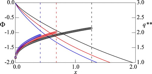
Figure 4. Computed $\mathrm{\Phi }$ (curve), $q^{\ast \ast }$ (circles), and $\overline{x}$ (broken lines) with $m=0.5$ for $\gamma =4$ (black), $\gamma =5$ (red), and $\gamma =6$ (blue). $q^{\ast \ast }$ is plotted only for the area where $G\left(x,\frac{\text{d}\mathrm{\Phi }}{\text{d}x}\right)>0$.

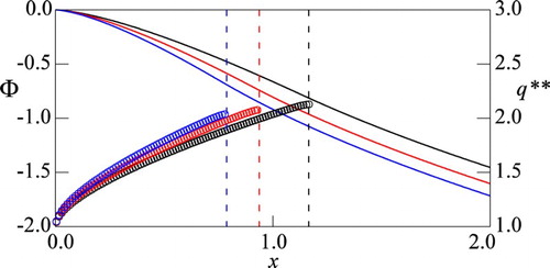
Table 1. Parameter values employed in numerical computation.

Model parameter	Parameter value
$r$	0.5
$\sigma$	0.2
$k$	0.3
$n$	−0.5, 0.5, or 2.0
$l$	0.6
$\beta$	1.0
$\gamma$	4.0, 5.0, or 6.0
$p$	2
$m$	−0.2 or 0.5
$\delta$	4.0
$\overline{q}$	1.0

Figures 1 and 2 plot the numerically computed $\mathrm{\Phi }$ and $q^{\ast \ast }$ for small $x>0$, respectively. The computational results reasonably agree with Proposition 4.6, verifying the theoretical analysis results. Figures 3 and 4 show the computed $\mathrm{\Phi }$, $q^{\ast \ast }$, and $\overline{x}$ for different values of $\gamma$ with $m=-0.2$ and $m=0.5$, respectively. Figures 3 and 4 validate Remark 4.1. In addition, the results show that Proposition 4.2 holds true for the singular-regular case, implying that the optimal control ${\eta }^{\ast }$ is a barrier type that is exerted so that $X_t\left(t\ge 0\right)$ is in $\left[0,\overline{x}\right]$ if $X_0\in \left[0,\overline{x}\right]$ as in the exactly solvable case.

Finally, as an advanced topic, validity of the asymptotic analysis results in Proposition 4.6 is examined for the Verhulst counterpart where the SDE (1) is replaced by (94) $\text{d}{X}_t=\left(r\right(1-X_{t-})-R(q_t\left)\right)X_{t-}\text{d}t+\sigma X_{t-}\text{d}{B}_t-X_{t-}^l\text{d}{\eta }_t.$(94) In the Verhulst counterpart (Equation (94)), the drift term is quadratic with respect to the solution. This model would serve as a more realistic mathematical model of the algae growth in which their deterministic growth rate is upper-bounded. Formal calculation analogous to that in Proposition 4.6 leads to the same asymptotic behaviour (Equation (86)). Figures 5 and 6 plot the computed $\mathrm{\Phi }$ and $q^{\ast }$ for small $x>0$, respectively. The computational results are close to those presented in Figures 1 and 2, and clearly demonstrate that the asymptotic results of Proposition 4.6 for the model with SDE (1) apply also to the model with the Verhulst-type SDE (94) having a more complicated coefficient.

Figure 5 Asymptotic analysis results for the value function $\mathrm{\Phi }$ and the optimal dam discharge $q^{\ast \ast }$ for the Verhulst counterpart with $n=-0.5$. Black: $m=-0.2$ and grey: $m=0.5$. •: Numerical solution and ⃝: Asymptotic result.

Figure 6 Asymptotic analysis results for the value function $\mathrm{\Phi }$ and the optimal dam discharge $q^{\ast \ast }$ for the Verhulst counterpart with $n=0.5$. Black: $m=-0.2$ and grey: $m=0.5$. •: Numerical solution and ⃝: Asymptotic result.

5. Conclusions

A stochastic control problem for finding the ecologically sound and fit-for purpose optimal policy to suppress bloom of the attached algae was formulated. The optimal control problem ultimately reduced to a boundary value problem of the HJB equation. The value function was characterized as a locally Lipschitz continuous viscosity solution to the HJB equation. The exactly solvable case subject to the uncontrolled dam discharge was firstly analysed, showing that the value function is the unique viscosity as well as classical solution to the HJB equation. In addition, parameter dependence of the optimal threshold to suppress the algae bloom was theoretically derived. The more realistic, regular-singular control case where the dam discharge is controlled was secondly analysed with the help of an asymptotic analysis technique. Parameter dependence of the optimal dam discharge was then analysed, implying impacts of the personality of the decision-maker on the optimal dam discharge during the early stage of the algae growth. Numerical computation of the HJB equation was finally carried out to verify the mathematical analysis results. The results presented in this paper would be helpful for comprehension and assessment of the algae growth dynamics and planning of their effective management policies.

In future research, we will consider a finite-horizon counterpart of the presented mathematical model where the parameters and coefficients such as the target dam discharge are time-dependent. This model is more realistic than the presented one, but an appropriate numerical technique will be necessary for its practical application. Utilizing the impulsive control [12,30] as an alternative to the singular one is also an interesting and practically meaningful research topic. Incorporating storage dynamics of the dam, which is temporally stochastic [8,45], would advance the mathematical modelling so that a more complicated dam operation policy can be handled. Along with the above-mentioned mathematical modelling, observations of dam discharge and algae growth in several Japanese rivers will be continued by the authors with the help of local fisheries cooperatives for deeper comprehension of their dynamics.

Acknowledgements

The authors thank Hii River Fishery Cooperatives for providing valuable comments on this research. The authors also thank the two Reviewers for their critical comments and valuable suggestions.

Disclosure statement

No potential conflict of interest was reported by the authors.

ORCID

Hidekazu Yoshioka http://orcid.org/0000-0002-5293-3246

Additional information

Funding

This work was supported by the Japan Society for the Promotion of Science [grant KAKENHI Numbers 17J09125, 17K15345]; The River Foundation [grant The River Fund Number 285311020]; Water Resources Environment Center [grant The WEC Applied Ecology Research Number 2016-02].

References

- E.J. Allen, Derivation of stochastic partial differential equations for size-and age-structured populations, J. Biol. Dyn. 3(1) (2009), pp. 73–86. doi: 10.1080/17513750802162754
- H. Al Motairi and M. Zervos, Irreversible capital accumulation with economic impact, Appl. Math. Opt. 75(3) (2017), pp. 525–551. doi: 10.1007/s00245-016-9341-9
- L.H. Alvarez, Singular stochastic control in the presence of a state-dependent yield structure, Stoch. Process. Appl. 86(2) (2000), pp. 323–343. doi: 10.1016/S0304-4149(99)00102-7
- P. Azcue and N. Muler, Stochastic Optimization in Insurance: A Dynamic Programming Approach, Springer, New York, 2014.
- R.K. Bansal, A Textbook of Fluid Mechanics and Hydraulic Machines. Laxmi Publications, India, 2005.
- B.J. Biggs, R.P. Ibbitt, and I.G. Jowett, Determination of flow regimes for protection of in-river values in New Zealand: an overview, Ecohydrol. Hydrobiol. 8(1) (2008), pp. 17–29. doi: 10.2478/v10104-009-0002-3
- S. Boulêtreau, F. Garabétian, S. Sauvage, and J.M. Sánchez-Pérez, Assessing the importance of a self-generated detachment process in river biofilm models, Freshwater Biol. 51(5) (2006), pp. 901–912. doi: 10.1111/j.1365-2427.2006.01541.x
- O. Boxma, D. Perry, W. Stadje, and S. Zacks, The M/G/1 queue with quasi-restricted accessibility, Stoch. Models. 25(1) (2009), pp. 151–196. doi: 10.1080/15326340802648878
- W.B. Buddendorf, I.A. Malcolm, J. Geris, M.E. Wilkinson, and C. Soulsby, Metrics to assess how longitudinal channel network connectivity and in-stream Atlantic salmon habitats are impacted by hydropower regulation, Hydrol. Process. 31(12) (2017), pp. 2132–2142. doi: 10.1002/hyp.11159
- J. Chevallier and B. Sévi, On the stochastic properties of carbon futures prices, Environ. Resour. Econ. 58(1) (2014), pp. 127–153. doi: 10.1007/s10640-013-9695-2
- T. Choulli, M. Taksar, and X.Y. Zhou, A diffusion model for optimal dividend distribution for a company with constraints on risk control, SIAM J. Control Opt. 41(6) (2003), pp. 1946–1979. doi: 10.1137/S0363012900382667
- L. Chu, T. Kompas, and Q. Grafton, Impulse controls and uncertainty in economics: method and application, Environ. Modell. Softw. 65 (2015), pp. 50–57. doi: 10.1016/j.envsoft.2014.11.027
- F. Coundoul, T. Bonometti, M. Graba, S. Sauvage, J.M. Sanchez Pérez, and F.Y. Moulin, Role of local flow conditions in river biofilm colonization and early growth, River Res. Appl. 31(3) (2015), pp. 350–367. doi: 10.1002/rra.2746
- M. Decamps, A. De Schepper, M. Goovaerts, Spectral decomposition of optimal asset-liability management, J. Econ. Dyn. Control. 33(3) (2009), pp. 710–724. doi: 10.1016/j.jedc.2008.09.002
- W.H. Fleming and H.M. Soner, Controlled Markov Processes and Viscosity Solutions, Springer Science+Business Media, New York, 2006.
- O. Fovet, G. Belaud, X. Litrico, S. Charpentier, C. Bertrand, A. Dauta, and C. Hugodot, Modelling periphyton in irrigation canals, Ecol. Model. 221(8) (2010), pp. 1153–1161. doi: 10.1016/j.ecolmodel.2010.01.002
- O. Fovet, G. Belaud, X. Litrico, S. Charpentier, C. Bertrand, P. Dollet, and C. Hugodot, A model for fixed algae management in open channels using flushing flows, River Res. Appl. 28(7) (2012), pp. 960–972. doi: 10.1002/rra.1495
- V. Frossard, S. Versanne-Janodet, and L. Aleya, Factors supporting harmful macroalgal blooms in flowing waters: a 2-year study in the lower Ain River, France, Harmful Algae. 33 (2014), pp. 19–28. doi: 10.1016/j.hal.2014.01.001
- N.D. Gillett, Y. Pan, J.E. Asarian, and J. Kann, Spatial and temporal variability of river periphyton below a hypereutrophic lake and a series of dams, Sci. Total Environ. 541 (2016), pp. 1382–1392. doi: 10.1016/j.scitotenv.2015.10.048
- M. Grigoriu, Noise-induced transitions for random versions of Verhulst model, Prob. Eng. Mech. 38 (2014), pp. 136–142. doi: 10.1016/j.probengmech.2014.01.002
- X. Guo, J. Liu, and X.Y. Zhou, A constrained non-linear regular-singular stochastic control problem, with applications, Stoch. Process Appl 109(2) (2004), 167–187. doi: 10.1016/j.spa.2003.09.008
- X. Guo and M. Zervos, Optimal execution with multiplicative price impact, SIAM J. Financ. Math. 6(1) (2015), pp. 281–306. doi: 10.1137/120894622
- D.D. Hart, B.J. Biggs, V.I. Nikora, and C.A. Flinders, Flow effects on periphyton patches and their ecological consequences in a New Zealand river, Freshw. Biol. 58(8) (2013), pp. 1588–1602. doi: 10.1111/fwb.12147
- Hattori, N., Uchida, A., Sano, M., and Murakami, T. Sensory analysis of the taste of Ayu sampled from different river environments, Food Sci. Technol. Res. 19(3) (2013), pp. 479–483. doi: 10.3136/fstr.19.479
- L. He and Z. Liang, Optimal financing and dividend control of the insurance company with fixed and proportional transaction costs, Insur. Math. Econ. 44(1) (2009), pp. 88–94. doi: 10.1016/j.insmatheco.2008.10.001
- B.H. Højgaard and M. Taksar, Controlling risk exposure and dividends payout schemes: insurance company example, Math. Financ. 9(2) (1999), pp. 153–182. doi: 10.1111/1467-9965.00066
- X. Huang, P. He, and W. Zhang, A cooperative differential game of transboundary industrial pollution between two regions. J. Clean Prod. 120 (2016), pp. 43–52. doi: 10.1016/j.jclepro.2015.10.095
- B.G. Jang, S. Park, and Y. Rhee, Optimal retirement with unemployment risks, J. Bank Finance. 37(9) (2013), pp. 3585–3604. doi: 10.1016/j.jbankfin.2013.05.017
- F.A. Khan and A.A. Ansari, Eutrophication: an ecological vision, Bot. Rev. 71(4) (2005), pp. 449–482. doi: 10.1663/0006-8101(2005)071[0449:EAEV]2.0.CO;2
- T. Kompas and L. Chu, Comparing approximation techniques to continuous-time stochastic dynamic programming problems: applications to natural resource modelling, Environ. Modell. Softw. 38 (2012), pp. 1–12. doi: 10.1016/j.envsoft.2012.04.002
- S.T. Larned and C. Kilroy, Effects of Didymosphenia geminata removal on river macroinvertebrate communities, J. Freshw. Ecol. 29(3) (2014), pp. 345–362. doi: 10.1080/02705060.2014.898595
- J. Lessard, D.M. Hicks, T.H. Snelder, D.B. Arscott, S.T. Larned, D. Booker, and A.M. Suren, Dam design can impede adaptive management of environmental flows: a case study from the Opuha Dam, New Zealand, Environ. Manage. 51(2) (2013), pp. 459–473. doi: 10.1007/s00267-012-9971-x
- P.L. Lions and A.S. Sznitman, Stochastic differential equations with reflecting boundary conditions. Commun. Pure Appl. Math. 37(4) (1984), pp. 511–537. doi: 10.1002/cpa.3160370408
- X. Litrico, G. Belaud, and O. Fovet, Adaptive control of algae detachment in regulated canal networks. Proceedings of Networking, Sensing and Control (ICNSC), IEEE. 197–202, 2011.
- A. Maheu, A. St-Hilaire, D. Caissie, N. El-Jabi, G. Bourque, and D. Boisclair, A regional analysis of the impact of dams on water temperature in medium-size rivers in eastern Canada. Can. J. Fish. Aquat Sci. 73(12) (2016), pp. 1885–1897. doi: 10.1139/cjfas-2015-0486
- T.G. McAllister, S.A. Wood, and I. Hawes, The rise of toxic benthic Phormidium proliferations: a review of their taxonomy, distribution, toxin content and factors regulating prevalence and increased severity. Harmful Algae. 55 (2016), pp. 282–294. doi: 10.1016/j.hal.2016.04.002
- E. Meyer-Peter and R. Müller, Formulas for bed-load transport. International Association of Hydraulic Research, 2nd meeting, Stockholm, 39–64, 1948.
- H. Morimoto, Optimal dividend payments in the stochastic Ramsey model, Stoch. Process. Appl. 120(4) (2010), pp. 427–441. doi: 10.1016/j.spa.2010.01.001
- K. Nozaki, A. Uchida, Blooms of filamentous green algae in river ecosystem, Yahagi River Res. 4 (2000), pp. 159–168. (in Japanese)
- B. Øksendal and A. Sulem, Stochastic Control of Jump Diffusions, Springer-Verlag, Berlin, Heidelberg, 2007.
- J. Palczewski, R. Poulsen, K.R. Schenk-Hoppé, and H. Wang, Dynamic portfolio optimization with transaction costs and state-dependent drift, Eur. J. Oper. Res. 243(3) (2015), pp. 921–931. doi: 10.1016/j.ejor.2014.12.040
- A. Pascucci, PDE and Martingale Methods in Option Pricing, Springer-Verlag Italia, Milan, 2011.
- L.G. Perry, L.V. Reynolds, T.J. Beechie, M.J. Collins, and P.B. Shafroth, Incorporating climate change projections into riparian restoration planning and design, Ecohydrology. 2015, 8(5), pp. 863–879. doi: 10.1002/eco.1645
- H. Pham, Continuous-time Stochastic Control and Optimization with Financial Applications, Springer-Verlag, Berlin, Heidelberg, 2009.
- M. Pihlsgård, Loss rate asymptotics in a GI/G/1 queue with finite buffer, Stoch. Models. 2005, 21(4), pp. 913–931.
- V. Singh, Dam Breach Modeling Technology, Springer, Netherlands, 2013.
- G. Shim, and Y.H. Shin, An optimal job, consumption/leisure, and investment policy, Oper. Res. Lett. 42(2) (2014), pp. 145–149. doi: 10.1016/j.orl.2014.01.009
- I.B. Tahar, H.M. Soner, and N. Touzi, Merton problem with taxes: characterization, computation, and approximation. SIAM J. Financ. Math. 1(1) (2010), pp. 366–395. doi: 10.1137/080742178
- A. Taleb, N. Belaidi, and J. Gagneur, Water quality before and after dam building on a heavily polluted river in semi-arid Algeria. River Res. Appl. 20(8) (2004), pp. 943–956. doi: 10.1002/rra.800
- S. Thonhauser and H. Albrecher, Optimal dividend strategies for a compound Poisson process under transaction costs and power utility, Stoch. Models. 27(1) (2011), pp. 120–140. doi: 10.1080/15326349.2011.542734
- T. Tsujimoto, and T. Tashiro, Application of population dynamics modeling to habitat evaluation -growth of some species of attached algae and its detachment by transported sediment. Hydroécol. Appl. 14 (2004), pp. 161–174. doi: 10.1051/hydro:2004010
- H. Xiang, B. Liu, and Z. Li, Verification theory and approximate optimal harvesting strategy for a stochastic competitive ecosystem subject to Lévy noise. J. Dyn. Control Syst. 23(4) (2017), pp. 753–777. doi: 10.1007/s10883-017-9362-y
- Y. Yaegashi, H. Yoshioka, K. Unami, and M. Fujihara, Numerical simulation of a Hamilton-Jacobi-Bellman equation for optimal management strategy of released Plecoglossus altivelis in river systems, in Model Design and Simulation Analysis: Communications in Computer and Information Science, 603, S.D. Chi and S.Y. Ohn, eds., Springer Science+Business Media Singapore, Singapore, 2016, pp. 91–101.
- Y. Yaegashi, H. Yoshioka, K. Unami, and M. Fujihara, An optimal management strategy for stochastic population dynamics of released Plecoglossus altivelis in rivers. Int. J. Mod. Simul. Sci. Comput. 8(2) (2017a), 1750039, 16pp. doi: 10.1142/S1793962317500398
- Y. Yaegashi, H. Yoshioka, K. Unami, and M. Fujihara, Numerical approximation of singular stochastic control models of extermination strategy for the population of harmful animals. Proceedings of Computational Engineering Conference JSCES, 22, 2017 May. 2017b, Paper No D-05-7, 6pp. (in Japanese with English Abstract)
- H. Yoshioka, T. Shirai, and D. Tagami, Viscosity solutions of a mathematical model for upstream migration of potamodromous fish, 12th SDEWES Conference, October 4–8, 2017, Dubrovnik, Croatia. (Accepted).
- H. Yoshioka, K. Unami, and M. Fujihara, Mathematical analysis on a conforming finite element scheme for advection-dispersion-decay equations on connected graphs. J. JSCE A2. 70(2) (2014), pp. I_265–I_276. doi: 10.2208/jscejam.70.I_265
- H. Yoshioka and Y. Yaegashi, Mathematical and numerical modeling of the dam discharge operation policy to suppress bloom of harmful attached algae on river bed just downstream of a dam. Adv. River Eng. JSCE. 23 (2017), pp. 561–566. (in Japanese with English Abstract)
- H. Yoshioka and Y. Yaegashi, Optimization model to start harvesting in stochastic aquaculture system, App. Stoch. Models Bus. 33(5) (2017), pp. 476–493. doi: 10.1002/asmb.2250
- H. Yoshioka and Y. Yaegashi, Robust stochastic control modeling of dam discharge to suppress overgrowth of downstream harmful algae, Appl. Stoch. Models Bus. (under review)
- C. Yuan, X. Mao, and J. Lygeros, Stochastic hybrid delay population dynamics: well-posed models and extinction, J. Biol. Dyn. 3(1) (2009), pp. 1–21. doi: 10.1080/17513750802020804
- J. Zhu, and H. Yang, Optimal capital injection and dividend distribution for growth restricted diffusion models with bankruptcy. Insur. Math. Econ. 70 (2016), pp. 259–271. doi: 10.1016/j.insmatheco.2016.05.011
- J. Zou, Z. Zhang, and J. Zhang, Optimal dividend payouts under jump-diffusion risk processes. Stoch. Models. 25(2) (2009), pp. 332–347. doi: 10.1080/15326340902870133