Hierarchical competition models with the Allee effect III: multispecies

ABSTRACT

A general notion of the Allee effect for higher dimensional triangular maps is proposed. A global dynamics theory is established. The theory is applied to multi-species hierarchical models. Then we provide a detailed study of the global dynamics of three-species Ricker competition models with the Allee effect. Regions of extinction, exclusion and coexistence are identified.

KEYWORDS:

• Allee effect
• triangular maps
• competition models
• omega limit set
• global dynamics
• invariant manifolds

AMS SUBJECT CLASSIFICATIONS:

• 39A11
• 92D25

1. Introduction

The global dynamics of triangular maps have been investigated by Cima et al. [9] and Balreira et al. [5]. In [9], a special class of triangular maps was investigated, while in [5] a general class of triangular maps was thoroughly studied. In the latter study, the non-hyperbolic cases were not fully understood and many open questions are still unresolved. A complete study was done of the non-hyperbolic case under the assumption that the centre manifolds of the non-hyperbolic fixed points are stable. Unfortunately, this is not the case for most competition models [3, 4] in which the centre manifold is semi-stable. Hence it is desirable to remove this condition.

In this paper, we provide a complete analysis of a class of triangular maps. Then we apply these results to hierarchical competition models with the Allee effect that are represented by triangular maps. By this we complete the stability analysis that was initiated in Assas et al. [3, 4].

By a hierarchical model, we mean a dynamical system model with a networked hierarchy of state variables rather than the random parameter models of statistics [6, 7, 12, 21, 23, 24].

In hierarchical models, it is assumed that one of the species is ‘silverback’ species that gets first choice of the resources and whose is limited only by its own intraspecific competition, while the other species are less dominant and their growth are limited by the presence of species that are above them in the hierarchy.

The Allee effect was introduced by Allee [1] and was popularized by the book of Courchamp et al. [11]. It is a phenomenon in biology that is characterized by a positive correlation between population density and its per capita growth rate. One can make a distinction between the strong Allee effect and the weak Allee effect: a strong Allee effect refers to a population that exhibits a ‘critical size or density’ below which the population declines to extinction, while a weak Allee effect refers to a population that lacks a ‘critical density’, but where, at lower densities, the population growth rate rises with increasing densities [4, 11]. With few exceptions, the literature on the Allee effect is exclusively for single-species [8, 14, 15, 18–20, 28–30, 32]. Allee effect for two species was considered in Livadiotis-Elaydi [27], Livadiotis et al. [25], Assas et al. [3], Livadiotis et al. [26], Jang [22] and Cushing [13].

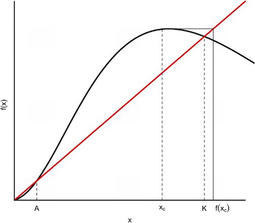
In Figure 1, we plot the fitness or the growth rate per capita of a population $x(t+1)/x\left(t\right)$ versus its size or density $x\left(t\right)$ to illustrate the differences among models with no Allee effect (brown), with weak Allee effect (blue) and with strong Allee effect (green). For the Allee effect models, with weak or strong, the growth rate increases, initially, as the population size or density increases. In this paper, we only consider the strong Allee effect which is characterized by the existence of an extinction region. Figure 1 illustrates the strong Allee effect of a single species. There are three fixed points, $x_1^{\ast }=0$ (extinction), $x_2^{\ast }=A$ (the Allee threshold) and $x_3^{\ast }=K$ (the carrying capacity). If the initial size $x_0$ of the population is less than A, then its orbits converge to 0 and the population, eventually, goes to extinction.

Figure 1. The graph shows the growth rate per capita as a function of the density (size) of the population. The three curves represent the cases of no Allee effect (brown), weak Allee effect (blue) and strong Allee effect (green).

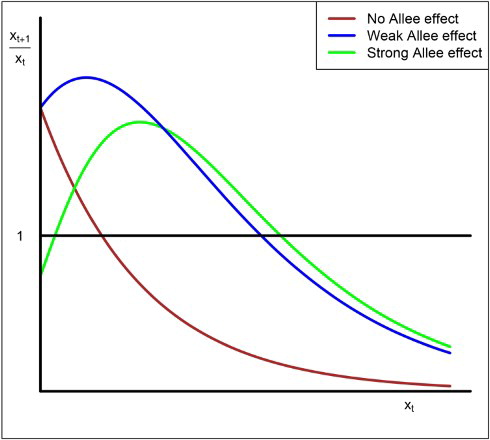
Figure 2. In the strong Allee case, there are three fixed points, $x_1^{\ast }=0$ (extinction), $x_2^{\ast }=A>0$ (the Allee threshold) and $x_3^{\ast }=K>A$ (the carrying capacity). If the initial size $x_0$ of the population is less than A, then its orbits converge to 0 and the population goes to extinction.

1.1. Causes of the Allee effect

Mechanisms that cause the Allee effect may include mate limitations, that is, difficulty in finding mates, cooperative breeding and cooperative defense [11]. Another mechanism that causes the Allee effect is predator saturation, where it is assumed that a constant level of predation is present. Moreover, our model does not require that the predator be just one in number, acting on all species, but that they could be many, even different ones for different species in the hierarchy. The model also assumes that all species in the hierarchy possess the Allee effect induced by predator satiation (saturation). An example of this phenomenon is the case of cicadas that would supply predators with enough cicadas to eat until they are weary of eating, which gives the remaining cicadas a chance to escape predation.

1.2. Allee effect in higher dimensions

We define the Allee affect as follows:

Definition 1.1

Let $F:{\mathbb{R}}_{+}^n\to {\mathbb{R}}_{+}^n$ be a continuous map, then we say that F possesses the strong Allee effect if there is an extinction region, in which all species go to extinction, and persistent regions in which some or all of the species survive.

Let $F=(f_1,f_2,\dots ,f_n),X\left(t\right)=\left(x_1\right(t),x_2(t),\dots ,x_n(t\left)\right)$ and (1.1) $X(t+1)=F\left(X\right(t\left)\right)$(1.1) be the associated difference equation. Then from the above definition, system (1.1(1.1) $X(t+1)=F\left(X\right(t\left)\right)$(1.1) ) has the strong Allee effect if there is an open neighbourhood G of the origin, which is assumed to be a fixed point, such that if $X_0\in G$, then $\underset{t\to \mathrm{\infty }}{lim}X\left(t\right)=0$. The set G will be called the immediate region of extinction.

2. Triangular maps

Here we consider a class of continuous maps $F:{\mathbb{R}}_{+}^n\to {\mathbb{R}}_{+}^n$, where $F\left(X\right)=\left(f_1\right(x_1),f_2(x_1,x_2),\dots ,f_n(x_1,x_2,\dots ,x_n\left)\right)$, where $X=(x_1,x_2,\dots ,x_n)\in {\mathbb{R}}_{+}^n$ and $x_i\ge 0$, $1\le i\le n$.

Our maps are of Kolmogorov type, that is, $f_1\left(x_1\right)=x_1{g}_1\left(x_1\right),f_2(x_1,x_2)=x_2{g}_2(x_1,x_2),\dots ,f_n(x_1,x_2,\dots ,x_n)=x_n{g}_n(x_1,x_2,\dots ,x_n).$

A hyperspace $H_k$ of dimension $k\le n$ is defined as $H_k=\left\{\right(x_1,x_2,\dots ,x_n):x_{i1},x_{i2},\dots ,x_{ik},>0$ for some $i_1,i_2,\dots ,i_k,$ and the remaining components are all zeros$\}$. Note that each hyperspace is invariant. A fibre ${\mathcal{F}}_k$ in $H_k$ is a one-dimensional subset of $H_k$ with all the positive components except one constitute a fixed point in $H_{k-1}$. For instance, if $H_k=\left\{\right(x_1,x_2,\dots ,x_k,0,\dots ,0):x_i>0,1\le i\le k\}$, then one of the fibres may be given by $\mathcal{F}=\{x_1^{\ast },x_2^{\ast },\dots ,x_{k-1}^{\ast },x_k,0,\dots ,0\}$, where $(x_1^{\ast },x_2^{\ast },\dots ,x_{k-1}^{\ast },0,\dots ,0)$ is a fixed point in $H_{k-1}$. The dynamics on this fibre $\mathcal{F}$ is determined by the map $f_k$. The map $f_k$ on $\mathcal{F}$ may be regarded as a one dimensional map, since $F(x_1^{\ast },x_2^{\ast },\dots ,x_{k-1}^{\ast },x_k,0\dots ,0)=(x_1^{\ast },x_2^{\ast },\dots ,x_{k-1}^{\ast },f_k(x_1^{\ast },x_2^{\ast },\dots ,x_{k-1}^{\ast },x_k),0\dots ,0)$. Hence the dynamics on ${\mathcal{F}}_k$ is determined by the one-dimensional map ${\tilde{f}}_k\left(x_k\right)=f_k(x_1^{\ast },x_2^{\ast },\dots ,x_{k-1}^{\ast },x_k)$.

Now to find all the fix points, we let $f_1\left(x_1\right)=x_1,f_2(x_1,x_2)=x_2,\dots ,f_n(x_1,x_2,\dots ,x_n)=x_n$. The intersections of these surfaces give the fixed points of the difference equation. These equations are called isoclines of the system.

If the maps are of Kolmogorov type, then the isoclines are given by (2.1) $g_i(x_1,x_2,\dots ,x_i)-1=0,1\le i\le n.$(2.1)

The following crucial one-dimensional result due to Coppel [10] was rediscovered by Sharkovsky et al. [31], Elaydi and Sacker [18] and was reported in the book of Alseda et al. [2].

Theorem 2.1

[10],[18]

Let $f:\mathbb{R}\to \mathbb{R}$ be a continuous map on the reals such that every orbit is bounded. Then every orbit converges to a fixed point f if and only if there are no periodic orbits of prime period 2 on any fibre.

In the sequel, we will make the following assumptions.

Assumption

$H_1$

All orbits are bounded.

Assumption

$H_2$

There are no periodic orbits of prime period 2 on any fibre.

Assumption

$H_3$

The isoclines are polynomials of finite degree.

Note that assumption $\left(H_3\right)$ implies that there are finitely many fixed points on each fibre.

Corollary 2.1

For any continuous triangular map on ${\mathbb{R}}_{+}^n$, if Assumptions $\left(H_1\right)$ and $\left(H_2\right)$ hold true, then every orbit on a fibre must converge to a fixed point on the fibre.

Proof.

Note that on each fibre ${\mathcal{F}}_k$, in a hyperspace $H_k$ of dimension k, the dynamics is determined by the one dimensional map ${\tilde{F}}_k:{\mathbb{R}}_{+}^1\to {\mathbb{R}}_{+}^1$, where ${\tilde{F}}_k\left(x_k\right)=F(x_1^{\ast },x_2^{\ast },\dots ,x_{k-1}^{\ast },x_k)$. Hence one may apply Theorem 1 (in Coppel [10] or Elaydi-Sacker [18]) to obtain the conclusion of the Corollary.

The main result in this section now follows.

Theorem 2.2

Let $F:{\mathbb{R}}_{+}^n\to {\mathbb{R}}_{+}^n$ be a continuous triangle map of Kolmogorov-type such that Assumptions $\left(H_1\right)$, $\left(H_2\right)$ and $\left(H_3\right)$ hold true. Then every orbit converges to a fixed point in ${\mathbb{R}}_{+}^n$.

To facilitate the proof of this theorem, we first recall the definition of the omega limit set $\omega \left(X\right)$ of a point $X\in {\mathbb{R}}_{+}^n:\omega \left(X\right)=\{P\in {\mathbb{R}}_{+}^n:F^{n_i}(X)\to P\mathrm{as}{n}_i\to \mathrm{\infty }$ for some subsequence $\left\{n_i\right\}$ of the set of positive integers$\}$. If the orbit of X is bounded, then $\omega \left(X\right)$ is non-empty, closed and invariant [16, 17].

Proof.

Assume $\left(H_1\right)$, $\left(H_2\right)$ and $\left(H_3\right)$. Let $X\in {\mathbb{R}}_{+}^k$. Then $\omega \left(X\right)$ lies on the fibre $\mathcal{F}=\left\{\right(x_1^{\ast },x_2^{\ast },\dots ,x_{n-1}^{\ast },x_n):f_1(x_1^{\ast })=x_1^{\ast },f_2(x_1^{\ast },x_2^{\ast })=(x_1^{\ast },x_2^{\ast }),\dots ,f_{n-1}(x_1^{\ast },x_2^{\ast },\dots ,x_{n-1}^{\ast })=(x_1^{\ast },x_2^{\ast },\dots ,x_{n-1}^{\ast }\left)\right\}$.

Let $P=(x_1^{\ast },x_2^{\ast },\dots ,x_{n-1}^{\ast },u)\in \omega \left(X\right)$. Then $F\left(P\right)=(x_1^{\ast },x_2^{\ast },\dots ,f_n(x_1^{\ast },x_2^{\ast },\dots ,x_{n-1}^{\ast },u\left)\right)$ is determined by the one-dimensional map $\tilde{f}:{\mathcal{F}}_n\to {\mathcal{F}}_n$, with $\tilde{f}\left(u\right)=f_n(x_1^{\ast },x_2^{\ast },\dots ,x_{n-1}^{\ast },u)$. There are two cases to consider.

Case 1: P is not a fixed point. In this case, by Theorem 2.1, under $\tilde{f}$, the orbit of P must converge to a fixed point $u=u^{\ast }$ on ${\mathcal{F}}_n$. Since $\omega \left(X\right)$ is closed and invariant, it follows that $X^{\ast }=(x_1^{\ast },x_2^{\ast },\dots ,x_{n-1}^{\ast },u)\in \omega \left(X\right)$. By Assumption $\left(H_3\right)$, the isocline $g_n(x_1^{\ast },x_2^{\ast },\dots ,x_{n-1}^{\ast },x_n)=1$ has finitely many roots, and hence there are only finite many fixed points on the fibre ${\mathcal{F}}_n$. Let $(X_1^{\ast },X_2^{\ast },\dots ,X_n)$ be the fixed points on the fibre ${\mathcal{F}}_n$. Then $X_i^{\ast }=(x_1^{\ast },x_2^{\ast },\dots ,x_{n-1}^{\ast },u)$. Thus the isocline $g_n-1=0$ may be written as $g_n-1=\gamma (u-u_1^{\ast })(u-u_2^{\ast })\dots (u-u_m^{\ast })=0$.

Now $u_{t+1}>u_t$ if $\tilde{f}\left(u\right)=ug\left(u\right)>u$ or $g\left(u\right)-1>0$, and $u_{t+1}<u_t$ if $g\left(u\right)-1<0$. Thus between the fixed points on the fibre ${\mathcal{F}}_n$, orbits are either increasing or decreasing depending on the location of u. Hence on the fibre ${\mathcal{F}}_n$, the fixed point $X_i^{\ast }=(x_1^{\ast },x_2^{\ast },\dots ,x_{n-1}^{\ast },u^{\ast })\in \omega \left(X\right)$ is either asymptotically stable or semi-stable. Moreover, $X^{\ast }$ must have a stable manifold or a semi-stable manifold of codimension one. In either case, the immediate basin of attraction of $X^{\ast }$ contains a point in the orbit of X. Hence $\omega \left(X\right)=X^{\ast }$, and consequently the orbit of X converges to $X^{\ast }$.

Case 2: Finally, assume that P is a fixed point of F. If Z is semi-stable or asymptotically stable, then as above, we have $\omega \left(X\right)=P$. On the other hand, if P is unstable, then there is a subsequence $F^{n_i}\left(X\right)\to Y\mathrm{as}{n}_i\to \mathrm{\infty }$ for some subsequence $\left\{n_i\right\}$, where Y lies on the unstable manifold on the fibre ${\mathcal{F}}_n$ of P. By Corollary 2.1, the orbit of Y must converge to a fixed point $Y^{\ast }$ on the fibre ${\mathcal{F}}_n$, which is either asymptotically stable or semi-stable. In either case, we have $\omega \left(X\right)=Y^{\ast }$.

Up to this point, we have discussed the global dynamics of the general triangular maps without considering the Allee effect phenomenon. The following result provides conditions under which a triangular map possesses the strong Allee effect.

Lemma 2.1

Under Assumptions $\left(H_1\right)$, $\left(H_2\right)$ and $\left(H_3\right)$, a triangular map has the strong Allee effect if and only if the number of positive roots (counting repeated roots) of each isocline is even.

Proof.

Without loss of generality, let us consider the $x_1$-axis and assume that there are $2\ell$ positive roots $q_1^{\ast }<q_2^{\ast }<\cdots <q_{2\ell }^{\ast }$ of the isocline equation $g_1\left(x_1\right)-1=0$. Hence orbits on the $x_1$-axis are decreasing if $x_1(t+1)=x_1\left(t\right)g_1\left(x_1\right(t\left)\right)>x_1\left(t\right)$ or $p_1\left(x_1\right)=g_1\left(x_1\right)-1=(x_1-q_1^{\ast })(x_1-q_2^{\ast })\cdots (x_1-q_{2\ell }^{\ast })>0$ and increasing if $p_1\left(x_1\right)=(x_1-q_1^{\ast })(x_1-q_2^{\ast })\cdots (x_1-q_{2\ell }^{\ast })<0$. Thus if $0<x_0<q_1^{\ast }$, then $p_1\left(x_0\right)>0$. Therefore, the orbit of $x_0$ must decrease and by Theorem 2.2, it must converge to the origin. Hence, the origin is asymptotically stable. Moreover, if $q_1<x_0<q_2^{\ast }$, then $p_1\left(x_0\right)<0$ and hence, the orbit of $x_0$ must increase and by Theorem 2.2, it must converge to $q_2^{\ast }$. If $q_2^{\ast }<x_0<q_3^{\ast }$, then $p_1\left(x_0\right)>0$, and thus the orbit of $x_0$ must decrease and by Theorem 2.2, it must converge to $q_2^{\ast }$. Hence, $q_1^{\ast }$ is unstable (a repeller) and $q_2^{\ast }$ is asymptotically stable. Inductively, one may show that $q_{2m}^{\ast }$ is asymptotically stable, while $q_{2m+1}^{\ast }$ is unstable. Hence there is an extinction region, in which also species would perish, and persistent regions in which some or all species survive, and consequently, the map F has the strong Allee effect.

In the following section, we will apply our general results to a specific class of maps that models hierarchical competition models with the Allee effect.

3. Hierarchical models with the Allee effect

We propose the following general hierarchical model of the Allee effect of the Ricker type. (3.1) $\left\{\begin{array}{rl}{x}_1(t+1)& =x_1\left(t\right)\exp (r_1-x_1(t\left)\right)\exp \left(-\frac{m_1}{[1+s_1{x}_1(t){]}^{{\ell }_1}}\right)\\ x_2(t+1)& =x_2\left(t\right)\exp (r_2-x_2(t)-b_{21}{x}_1(t\left)\right)\exp \left(-\frac{m_2}{[1+s_2{x}_2(t){]}^{{\ell }_2}}\right)\\ & ⋮\\ x_n(t+1)& =x_n\left(t\right)\exp \left(r_n-x_n\left(t\right)-\sum _{i=1}^{n-1}{b}_{ni}{x}_i\left(t\right)\right)\exp \left(-\frac{m_n}{[1+s_n{x}_n(t){]}^{{\ell }_n}}\right)\end{array}\right.,$(3.1) where $r_i$ is the intrinsic growth rate for species $x_i$. For $1\le i\le n-1,2\le j\le n$, $b_{ij}>0$ are the interspecific parameters (between species $x_i$ and $x_j$), $m_j>0$ is the predation intensity against species $x_j$ and $s_j>0$ is the prey handling time. The Allee effect is assumed to be caused by predator saturation and is represented by the terms $\text{exp}(-m_j/[1+s_j{x}_j(t){]}^{{\ell }_j})$, where the exponent ${\ell }_j\ge 1$ reflects the decreasing effect of predation on the growth of the prey. When ${\ell }_j=1$, the above model reduces to the classical Allee effect model. As ${\ell }_j$ increases, the impact of Allee effect on the growth of the prey decreases and when ${\ell }_j$ goes to ∞, the Allee effect term disappears and our model reduces to the classical Ricker model.

Note that in order for each of the species $x_i$ to have the strong Allee effect, the number of positive roots of the isocline equation (counting repeated roots) must be even.

In the sequel, we will focus on the 3-species model where we assume that $l_i=1$ for i=1,2,3. (3.2) $\left\{\begin{array}{rl}x(t+1)& =x\left(t\right)\exp (r_1-x(t\left)\right)\exp \left(-\frac{m_1}{1+s_{1}x\left(t\right)}\right)\\ y(t+1)& =y\left(t\right)\exp (r_2-y(t)-b_{21}x(t\left)\right)\exp \left(-\frac{m_2}{1+s_{2}y\left(t\right)}\right)\\ z(t+1)& =z\left(t\right)\exp (r_3-z(t)-b_{31}x(t)-b_{32}y(t\left)\right)\exp \left(-\frac{m_3}{1+s_{3}z\left(t\right)}\right)\end{array}\right..$(3.2) Note that $r_i$ is the intrinsic growth rate for species $x_i,1\le i\le 3$, and $b_{21},b_{31},b_{32}>0$ are the interspecific parameters, $m_i>0$ is the predation intensity and $s_i>0$ is the prey handling time, $1\le i\le 3$. The terms $\text{exp}\left(-m_1/\right(1+s_{1}x\left)\right),\text{exp}\left(-m_2/\right(1+s_{2}x\left)\right),\text{exp}\left(-m_3/\right(1+s_{3}x\left)\right)$ are the Allee effect terms.

To insure that all species possess the strong Allee effect, we make the following assumption: for i=1,2,3 (3.3) $r_i{s}_i>1,m_i>r_i,(r_i{s}_i-1{)}^2-4(m_i-r_i)>0.$(3.3) In addition to the extinction fixed point (0,0,0), we have six fixed points on the three axis denoted by $(A_1,0,0),(K_1,0,0),(A_2,0,0,),(K_2,0,0),(A_3,0,0),(K_3,0,0,)$ where for $1\le i\le 3$, $A_i<K_i$ and $\begin{array}{rl}{A}_i& =\frac{(r_i{s}_i-1)-\sqrt{(r_i{s}_i-1{)}^2-4(m_i-r_i)}}{2s_i},\\ K_i& =\frac{(r_i{s}_i-1)+\sqrt{(r_i{s}_i-1{)}^2-4(m_i-r_i)}}{2s_i}.\end{array}$ In order to find all the possible fixed points, we derive the equations of the isoclines by putting $x(t+1)=x\left(t\right),y(t+1)=y\left(t\right),z(t+1)=z\left(t\right)$. The first isocline is (3.4) $r_1-x-\frac{m_1}{1+s_{1}x}=0.$(3.4) The two solutions are the planes $x_{-}=A_1$ and $x_{+}=K_1$ with (3.5) $x_{\pm }=\frac{r_1{s}_1-1\pm \sqrt{(r_1{s}_1-1{)}^2-4s_1(m_1-r_1)}}{2s_1}.$(3.5) The second isocline is (3.6) $r_2-y-b_{21}x-\frac{m_2}{1+s_{2}y}=0.$(3.6) The two solutions are the parabola (3.7) $y_{\pm }\left(x\right)=\frac{r_2{s}_2-s_2{b}_{21}x-1\pm \sqrt{(r_2{s}_2-s_2{b}_{21}x-1{)}^2-4s_2(m_2-r_2)-b_{21}x}}{2s_2}.$(3.7) We denote by $x_{1\max }$ the value of x for with Equation (3.6(3.6) $r_2-y-b_{21}x-\frac{m_2}{1+s_{2}y}=0.$(3.6) ) is maximized. When x=0, we get the points $y_{-}\left(0\right)=A_2$ and $y_{+}\left(0\right)=K_2$. If $x=A_2$, $y_{-}\left(A_1\right)$ will be denoted by $y_{1A_1}$ and $y_{+}\left(A_1\right)$ by $y_{2A_1}$. Likewise, when $x=K_2$, $y_{-}\left(K_1\right)$ will be denoted by $y_{1K_1}$ and $y_{+}\left(K_1\right)$ by $y_{2K_1}$.

The third isocline is (3.8) $r_3-z-b_{31}x-b_{32}y-\frac{m_3}{1+s_{3}z}=0.$(3.8) The two solutions are the paraboloids (3.9) $\begin{array}{rl}{z}_{\pm }(x,y)& =\frac{r_3{s}_3-s_3{b}_{31}x-s_3{b}_{32}y-1}{2s_3}\\ & \pm \frac{\sqrt{(r_3{s}_3-s_3{b}_{21}x-s_3{b}_{32}y-1{)}^2-4s_3(m_3-r_3)+s_3{b}_{31}x+s_3{b}_{32}y}}{2s_3}.\end{array}$(3.9) When x=y=0, we get the points $z_{-}(0,0)=A_3$ and $z_{+}(0,0)=K_3$.

When $x=A_1,y=y_{1A_1}$, we get the points $z_{-}(A_1,y_{1A_1})$, denoted by $z_{111}$, and $z_{+}(A_1,y_{1A_1})$, denoted by $z_{112}$, $z_{-}(A_1,y_{2A_1})$, denoted by $z_{121}$, and $z_{+}(A_1,y_{2A_1})$, denoted by $z_{122}$.

When $x=K_1,y=y_{1K_1}$, we get the points $z_{-}(K_1,y_{1K_1})$, denoted by $z_{211}$, and $z_{+}(K_1,y_{1K_1})$, denoted by $z_{212}$, $z_{-}(K_1,y_{2K_1})$, denoted by $z_{221}$, and $z_{+}(K_1,y_{2K_1})$, denoted by $z_{222}$.

3.1. Existence of fixed points

For the three-species model (3.2(3.2) $\left\{\begin{array}{rl}x(t+1)& =x\left(t\right)\exp (r_1-x(t\left)\right)\exp \left(-\frac{m_1}{1+s_{1}x\left(t\right)}\right)\\ y(t+1)& =y\left(t\right)\exp (r_2-y(t)-b_{21}x(t\left)\right)\exp \left(-\frac{m_2}{1+s_{2}y\left(t\right)}\right)\\ z(t+1)& =z\left(t\right)\exp (r_3-z(t)-b_{31}x(t)-b_{32}y(t\left)\right)\exp \left(-\frac{m_3}{1+s_{3}z\left(t\right)}\right)\end{array}\right..$(3.2) ), we have the extinction fixed point (0,0,0); on the x-axis, we have the Allee fixed threshold point $(A_1,0,0)$ and the carrying capacity fixed point $(K_1,0,0)$ for species x; on the y- and z -axes, we have similar fixed points $(0,A_2,0),(0,K_2,0)$ and $(0,0,A_3),(0,0,K_3)$ 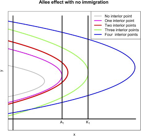respectively. The basin of attraction of one of the fixed points is the extinction exclusion region in which two species go to extinction. On each plane, there are at most four fixed points (see Figure 3 for an illustration). For instance, on the x−y plane, there are possibly the fixed points $(A_1,y_{1A_1},0),(A_1,y_{2A_1},0)$ on a fibre $x=A_1,y=y_{1A_1},z=t$ for $t\ge 0$, and $(K_1,y_{1K_1},0),(K_1,y_{2K_1},0)$ on a fibre $x=K_1,y=y_{1K_1},z=t$ for $t\ge 0$. Similarly on the y−z plane, we have fixed points $(0,A_2,y_{1A_2}),(0,A_2,y_{2A_2}),(0,K_2,y_{1K_2}),(0,K_2,y_{2K_2})$, and on the x−z plane, we have the fixed points $(A_1,0,z_{1A_1}),(A_1,0,z_{2A_1}),(K_1,0,z_{1K_1}),(K_1,0,z_{2K_1})$.

Figure 3. The graph illustrates the various scenarios that are determined by the location of $x_{1max}$. There are five scenarios where we have from zero to four interior fixed points.

On the $(x,y,z)$-space, there are at most eight (positive) coexistence fixed points. Hence the total number of coexistence points, where all species survive is $2^3=8$. For n-species, there are at most $3^n$ fixed points, and $2^n$ coexistence points, where all species survive (for n = 6, see Figure 6). In the sequel, we will give a detailed description of the stability of all fixed points.

3.2. Stability of the fixed points

The Jacobian matrix of system (3.2(3.2) $\left\{\begin{array}{rl}x(t+1)& =x\left(t\right)\exp (r_1-x(t\left)\right)\exp \left(-\frac{m_1}{1+s_{1}x\left(t\right)}\right)\\ y(t+1)& =y\left(t\right)\exp (r_2-y(t)-b_{21}x(t\left)\right)\exp \left(-\frac{m_2}{1+s_{2}y\left(t\right)}\right)\\ z(t+1)& =z\left(t\right)\exp (r_3-z(t)-b_{31}x(t)-b_{32}y(t\left)\right)\exp \left(-\frac{m_3}{1+s_{3}z\left(t\right)}\right)\end{array}\right..$(3.2) ) is given by (3.10) $J(x,y,x)=\left[\begin{array}{ccc}{J}_{11}& 0& 0\\ J_{21}& J_{22}& 0\\ J_{31}& J_{32}& J_{33}\end{array}\right],$(3.10) where $\begin{array}{rl}{J}_{11}& =\left(1-x+\frac{m_1{s}_{1}x}{(1+s_{1}x{)}^2}\right)e^{r_1-x-m_1/\left(1+s_{1}x\right)}\\ J_{21}& =-b_{21}y{e}^{r_2-y-b_{21}x-m_2/\left(1+s_{2}y\right)}\\ J_{22}& =\left(1-y+\frac{m_2{s}_{2}y}{(1+s_{2}y{)}^2}\right)e^{r_2-y-b_{2}x-m_2/\left(1+s_{2}y\right)}\\ J_{31}& =b_{31}z{e}^{r_3-z-b_{31}x-b_{32}y-m_3/\left(1+s_{2}z\right)}\\ J_{32}& =-b_{32}z{e}^{r_3-z-b_{31}x-b_{32}y-m_3/\left(1+s_{3}z\right)}\\ J_{33}& =\left(1-z+\frac{m_3{s}_{3}z}{(1+s_{3}z{)}^2}\right)e^{r_3-z-b_{31}x-b_{32}y-m_3/\left(1+s_{3}z\right)}.\end{array}$

3.2.1. Stability of the boundary fixed points

Let us start with the extinction fixed point $E_{000}=(0,0,0)$. Then we have $J(0,0,0)=\left[\begin{array}{ccc}{e}^{r_1-m_1}& 0& 0\\ 0& e^{r_2-m_2}& 0\\ 0& 0& e^{r_3-m_3}\end{array}\right].$ Since $r_i<m_i$ for $1\le i\le 3$, the extinction fixed points are asymptotically stable, where their stable manifolds lie on the three axes.

Next, we examine the stability of the fixed points on each axis. We start with the fixed points $E_{100}=(A_1,0,0),E_{010}=(0,A_2,0)$ and $E_{001}=(0,0,A_3)$. These are the Allee fixed points of each species in isolation of the other species. Now $J(A_1,0,0)=\left[\begin{array}{ccc}1-A_1+\frac{m_1{s}_2{A}_1}{(1+s_1{A}_1{)}^2}& 0& 0\\ 0& e^{r_2-b_{21}{A}_1-m_2}& 0\\ 0& 0& e^{r_3-b_{31}{A}_1-m_3}\end{array}\right].$ In [3], it was shown that the eigenvalue ${\lambda }_1=1-A_1+\frac{m_1{s}_2{A}_1}{(1+s_1{A}_1{)}^2}>1$ while from (3.3(3.3) $r_i{s}_i>1,m_i>r_i,(r_i{s}_i-1{)}^2-4(m_i-r_i)>0.$(3.3) ), the other eigenvalues are such that $\begin{array}{rl}{\lambda }_2& =e^{r_2-b_{21}{A}_1-m_2}<1\\ {\lambda }_3& =e^{r_3-b_{31}{A}_1-m_3}<1.\end{array}$ Hence $E_{100}$ is a saddle, where the unstable manifold lies on the x-axis and there are two stable manifolds: the lines $x=A_1,y=t,z=0$ and the line $x=A_1,y=0,z=t$ for $t\ge 0$.

One may make similar conclusions about the fixed points $E_{010}$ and $E_{001}$.

Next, we investigate the stability of the fixed points $E_{200}=(K_1,0,0),E_{020}=(0,K_2,0),E_{002}=(0,0,K_3)$. We have that $J(K_1,0,0)=\left[\begin{array}{ccc}1-K_1+\frac{m_1{s}_2{A}_1}{(1+s_1{K}_1{)}^2}& 0& 0\\ 0& e^{r_2-b_{21}{A}_1-m_2}& 0\\ 0& 0& e^{r_3-b_{31}{K}_1-m_3}\end{array}\right].$ In [3], it was shown that the eigenvalue $|{\lambda }_1|=1-K_1+\frac{m_1{s}_2{K}_1}{(1+s_1{A}_1{)}^2}<1\text{if }0<K_1-\frac{m_1{s}_2{K}_1}{(1+s_1{K}_1{)}^2}<2.$ The other two eigenvalues are such that $\begin{array}{rl}{\lambda }_2& =e^{r_2-b_{21}{K}_1-m_2}<1\\ {\lambda }_3& =e^{r_3-b_{31}{K}_1-m_3}<1.\end{array}$ Hence the fixed point $E_{200}$ is asymptotically stable, where one stable manifold lies on the x-axis and the other manifolds are given by the lines $x=K_1,y=t,z=0$ and the line $x=K_1,y=0,z=t$ for $t\ge 0$.

Similar conclusion may be obtained for $E_{020}$ and $E_{002}$, under the assumption (3.11) $0<K_i-\frac{m_1{s}_2{K}_I}{(1+s_1{K}_i{)}^2}<2,i=1,2,3.$(3.11)

3.2.2. Stability of the planar fixed points

Now, we investigate the stability of the fixed points in the x−y, x−z, and y−z planes, where one species is excluded, that is, one species goes to extinction. We will start with the x−y plane. A complete analysis of the dynamics in this plane was given in [3]. Here we are just giving a brief account on this.

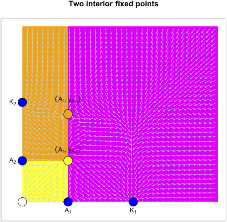
On the fibre $x=A_1,z=0$, we have either no fixed point, one fixed point $E_{110}=(A_1,y_{1A_1},0)$ or two fixed points $E_{110}$ and $E_{120}=(A_1,y_{2A_1},0)$, and on the fibre $x=K_1,z=0$, we have either no fixed point, one fixed point $E_{210}=(K_1,y_{1K_1},0)$ or two fixed points $E_{210}$ and $E_{220}=(K_1,y_{2K_1},0)$, see Figure 4. From [3] and by examining the third eigenvalue ${\lambda }_3$ in the Jacobian (3.10(3.10) $J(x,y,x)=\left[\begin{array}{ccc}{J}_{11}& 0& 0\\ J_{21}& J_{22}& 0\\ J_{31}& J_{32}& J_{33}\end{array}\right],$(3.10) ), we conclude the following:

1. $E_{110}$ is a saddle, where the two-dimensional unstable manifold lies on the x−y plane, and the stable manifold lies on the line $x=A_1,y=y_{1A_1},z=t$ for $t\ge 0$.

2. $E_{120}$ is a saddle with one dimensional unstable manifold tangent to the eigen vector $(t,y_{2A_1},0)$ for $t\ge 0$, one stable manifold on the fibre $x=A_1,y=t,z=0$ for $t\ge 0$ and one stable manifold that lies on the fibre $x=A_1,y=y_{2A_1},z=t$ for $t\ge 0$.

3. $E_{210}$ is a saddle with one-dimensional unstable manifold on the fibre $x=K_1,t=t,z=0$ for $t\ge 0$, one stable manifold tangent to the eigen vector $(t,y_{1k_1},0)$ and the other stable manifold lies on the fibre $x=K_1,y=y_{1K_1},z=t$ for $t\ge 0$.

4. $E_{220}$ is asymptotically stable.

In Figure 5, the phase space diagram for the non-negative x−y plane is shown, when there are only two fixed points that lie on the fibre $x=A_1,y=t,z=0$ for $t\ge 0$.

Figure 4. Phase space diagram depicting the dynamics of the three non-negative planes.

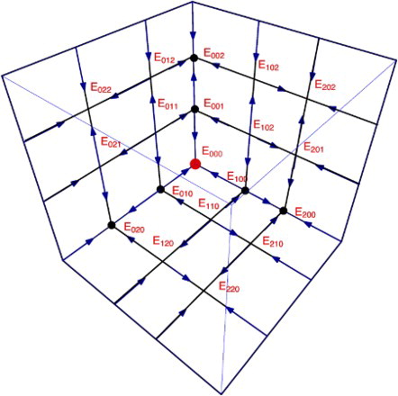
Figure 5. The phase space diagram in the case of two interior fixed points. There are three regions: extinction region (yellow), exclusion region of x (brown) and exclusion region of y (magenta).

Similar analysis can be given for the other two non-negative planes and will be omitted here for sake of brevity.

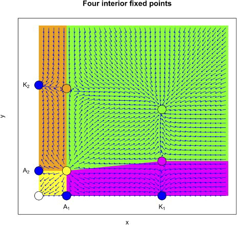
Figure 6. The phase space diagram of the x−y plane in the case of four interior fixed points. In the interior of the plane, there are four regions: extinction region (yellow), exclusion region of x (brown), exclusion region of y (magenta) and coexistence region (green).

3.2.3. Positive (interior) fixed points in the x−y−z space

Now, we focus on the dynamics in the non-negative orthant ${\mathbb{R}}_{+}^3$. The number of coexistence (positive) fixed points, where all the three species survive, is at most 8 (see Figure 7). Each line $x=x^{\ast },y=y^{\ast },z=t$, for $t\ge 0$, contains at most two fixed points, where for z=0, $(x^{\ast },y^{\ast })$ is either $E_{110},E_{120},E_{210}$ or $E_{220}$. Since there are 125 possible scenarios of the existence of fixed points in the interior of the three planes, we are going to limit our exposition to one case, namely, we assume that there are four in interior fixed points on each plane. Based on this assumption, it suffices to look at the third isocline where $x=x^{\ast }$ and $y=y^{\ast }$, where $x^{\ast }$ and $y=y^{\ast }$ are as defined above. The third isocline defined in (3.8(3.8) $r_3-z-b_{31}x-b_{32}y-\frac{m_3}{1+s_{3}z}=0.$(3.8) ) now becomes $r_3-z-b_{31}{x}^{\ast }-b_{32}{y}^{\ast }-\frac{m_3}{1+s_{3}z}=0,$ and (3.9(3.9) $\begin{array}{rl}{z}_{\pm }(x,y)& =\frac{r_3{s}_3-s_3{b}_{31}x-s_3{b}_{32}y-1}{2s_3}\\ & \pm \frac{\sqrt{(r_3{s}_3-s_3{b}_{21}x-s_3{b}_{32}y-1{)}^2-4s_3(m_3-r_3)+s_3{b}_{31}x+s_3{b}_{32}y}}{2s_3}.\end{array}$(3.9) ) becomes (3.12) $\begin{array}{rl}{z}_{\pm }(x^{\ast },y^{\ast })& =\frac{r_3{s}_3-s_3{b}_{31}{x}^{\ast }-s_3{b}_{32}{y}^{\ast }-1}{2s_3}\\ & \pm \frac{\sqrt{(r_3{s}_3-s_3{b}_{21}{x}^{\ast }-s_3{b}_{32}{y}^{\ast }-1{)}^2-4s_3(m_3-r_3)+s_3{b}_{31}{x}^{\ast }+s_3{b}_{32}{y}^{\ast }}}{2s_3}.\end{array}$(3.12) Since from (3.3(3.3) $r_i{s}_i>1,m_i>r_i,(r_i{s}_i-1{)}^2-4(m_i-r_i)>0.$(3.3) ), $m_3>r_3$, it follows that the quantity under the radical above is positive. Hence we have the following cases:

1. If (3.13) $s_3{b}_{31}{x}^{\ast }+s_3{b}_{32}{y}^{\ast }<r_3{s}_3-1,$(3.13) then there are two coexistence fixed points $(x^{\ast },y^{\ast },z_1(x^{\ast },y^{\ast }\left)\right)$ and $(x^{\ast },y^{\ast },z_2(x^{\ast },y^{\ast }\left)\right)$ that lie on the fibre $x=x^{\ast },y=y^{\ast },z=t$ for $t\ge 0$.

2. If (3.14) $s_3{b}_{31}{x}^{\ast }+s_3{b}_{32}{y}^{\ast }=r_3{s}_3-1,$(3.14) then there is only one coexistence fixed point $(x^{\ast },y^{\ast },z^{\ast })$ that lies on the fibre $x=x^{\ast },y=y^{\ast },z=t$ for $t\ge 0$.

3. If (3.15) $s_3{b}_{31}{x}^{\ast }+s_{3}b{t}_{32}{y}^{\ast }>r_3{s}_3-1,$(3.15) then there are no coexistence fixed point on the fibre $x=x^{\ast },y=y^{\ast },z=t$ for $t\ge 0$.

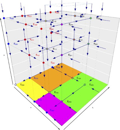
Figure 7. The figure shows the phase space diagram of the three species hierarchical Ricker model with the Allee effect. It shows the dynamics of every fixed point in the three planes, the axes, and the interior, from attractors, to repellers, and saddles.

We now turn our attention to the dynamics in case we have eight interior (positive) fixed points. We will denote for simplicity $z_{-}(x^{\ast },y^{\ast })$ as $E_{11i}=(A_1,y_{1A_1},z_{11i})$ on the fibre $x=A_1,y=y_{1A_1}$ and by $E_{12i}=(A_1,y_{2A_1},z_{12i})$, on the fibre $x=A_1,y=y_{2A_1}$, for i=1,2 . $z_{+}(x^{\ast },y^{\ast })$ will be denoted by $E_{21i}=(K_1,y_{1K_1},z_{11i})$ on the fibre $x=K_1,y=y_{1K_1}$ and by $E_{22i}=(K_1,y_{2K_1},z_{22i})$, on the fibre $x=K_1,y=y_{2K_1}$, for i=1,2.

1. On the fibre $x=A_1,y=y_{1A_1}$, there are two fixed points $E_{111}$, a repeller (unstable), and $E_{112}$, a saddle.

2. On the fibre $x=A_1,y=y_{2A_1}$, there are two fixed points $E_{121}$, a saddle with two-dimensional unstable manifold, and $E_{122}$, a saddle with two-dimensional stable manifold.

3. On the fibre $x=K_1,y=y_{1K_1}$, there are two fixed points $E_{211}$, a saddle with two-dimensional unstable manifold, and $E_{212}$, a saddle with two-dimensional stable manifold.

4. On the fibre $x=K_1,y=y_{2K_1}$, there are two fixed points $E_{221}$, a saddle with two-dimensional stable manifold, and $E_{222}$, asymptotically stable, whose basin of attraction is the coexistence region.

4. Conclusion

The dynamics of a 3-species competition model in which each species possesses the Allee effect has been investigated. The three species are assumed to be hierarchical in the sense that one species, x, is a ‘silverback’ species that gets first choice of the resources and whose growth rate is limited only by it is own intraspecific competition, while the other species, y and z, are less dominant and their growths are limited the presence of species that are above them. Hence species y growth rate is limited by species x and its own intraspecific competition, while species x growth rate is limited by both x and y and its own intraspecific competition. The Allee effect of each species is assumed to be caused by predator saturation.

There will be a region in ${\mathbb{R}}_{+}^3$ in which the three species go to extinction. In the extreme case, where there are no interior fixed points in ${\mathbb{R}}_{+}^3$, the extinction region is unbounded. At the other end of the spectrum, when there are eight interior fixed points in ${\mathbb{R}}_{+}^3$, the extinction region in ${\mathbb{R}}_{+}^3$ is bounded and a coexistence region exists. The coexistence region is this cases is the basin of attraction of the fixed points $E_{222}=(K_1,y_{2K_1},z_{222})$. Our analysis presents environmentalist with strategies for different scenarios. if one would like to save all three species, then inequality (3.11(3.11) $0<K_i-\frac{m_1{s}_2{K}_I}{(1+s_1{K}_i{)}^2}<2,i=1,2,3.$(3.11) ) should be satisfied at a starting point. This may be achieved, for instance, by increasing the growth rate $r_3$, of species z. On the other hand, of one wants to get rid of some species, for instance invasive undesirable invasive grass, then one may want inequality (3.13(3.13) $s_3{b}_{31}{x}^{\ast }+s_3{b}_{32}{y}^{\ast }<r_3{s}_3-1,$(3.13) ) or (3.14(3.14) $s_3{b}_{31}{x}^{\ast }+s_3{b}_{32}{y}^{\ast }=r_3{s}_3-1,$(3.14) ) satisfied.

Finally, to avoid the extinction of all species, one may use seeding or immigration to the species, see for instance [4].

Disclosure statement

No potential conflict of interest was reported by the author(s).

References

- W.C. Allee, The social life of animals, 3rd ed., William Heineman Ltd, London and Toronto, 1941.
- L. Alseda, J. Llibre and M. Misiurewicz, Combinatorial Dynamics and Entropy in Dimension One, World Scientific, Singapore, 2001.
- L. Assas, S. Elaydi, E. Kwessi, G. Livadiotis and D. Ribble, Hierarchical competition models with Allee effects, J. Biol. Dyn. 9(1) (2014), pp. 34–51.
- L. Assas, S. Elaydi, E. Kwessi, G. Livadiotis and B. Dennis, Hierarchical competition models with the Allee effect II: the case of immigration, J. Biol. Dyn. 9 (2015), pp. 288–316. doi: 10.1080/17513758.2015.1077999
- E. Balreira, S. Elaydi and R. Luis, Global dynamics of triangular maps, Nonlinear Anal. Theory Methods Appl. Ser. A, 104 (2014), pp. 75–83. doi: 10.1016/j.na.2014.03.019
- J. Best, C. Castillo-Chavez and A. Yakubu, Hierarchical competition in discrete time models with dispersal, Fields Institute Commun. 36 (2003), pp. 59–72.
- K.W. Blayneh, Hierarchical size-structured population models, Dyn. Syst. Appl. 9 (2000), pp. 527–539.
- J. Brashares, J. Werner and A. Sinclair, Social meltdown in the demise of an island endemic: Allee effects and the Vancouver island Marmot, J. Anim. Biol. 79 (2010), pp. 965–973.
- A. Cima, A. Gasull and V. Manosa, Basin of attraction of triangular maps with applications, J. Differ. Equ. Appl. 20 (2014), pp. 423–437. doi: 10.1080/10236198.2013.852187
- W.A. Coppel, The solution of equations by iteration, Math. Proc. Cambridge 51 (1955), pp. 41–43. doi: 10.1017/S030500410002990X
- F. Courchamp, L. Berec and J. Gascoigne, Allee Effects in Ecology and Conversation, Oxford University Press, Oxford, UK, 2008.
- J. Cushing, The dynamics of hierarchical age-structured populations, J. Math. Biol. 32 (1994), pp. 705–729. doi: 10.1007/BF00163023
- J. Cushing, Backward bifurcations and strong Allee effects in matrix models for the dynamics of structural populations, J. Biol. Dyn. 8 (2014), pp. 57–73. doi: 10.1080/17513758.2014.899638
- J.M. Cushing and J. Hudson, Evolutionary dynamics and strong Allee effect, J. Biol. Dyn. 6(2) (2012), pp. 941–958. doi: 10.1080/17513758.2012.697196
- B. Dennis, Allee effects: population growth, critical density, and the chance of extinction, Nat. Resour. Model, 3 (1989), pp. 481–538. doi: 10.1111/j.1939-7445.1989.tb00119.x
- S. Elaydi, Discrete Chaos, 2nd edn, Chapman & Hall/CRC, London, UK, 2008.
- S. Elaydi, An Introduction to Difference Equations, 3rd edn., Springer Science+Business Media, Inc., Berlin, Germany, 2005.
- S. Elaydi and R.J. Sacker, Population models with Allee effect: a new model, J. Biol. Dyn. 4 (2010), pp. 397–408. doi: 10.1080/17513750903377434
- M.S. Fowler and G.D. Ruxton, Population dynamic consequences of Allee effects, J. Theor. Biol. 215 (2002), pp. 39–46. doi: 10.1006/jtbi.2001.2486
- G.R.J. Graut, K. Goldring, F. Grogan, C. Haskell and R.J. Sacker, Difference equations with the Allee effect and the periodic sigmoid Beverson–Holt equation revisited, J. Biol. Dyn. 00 (2012), pp. 57–730.
- S.M. Henson and J.M. Cushing, Hierarchical models of interspecific competition: scramble versus contest, J. Math. Biol., 34 (1996), pp. 755–772. doi: 10.1007/BF00161518
- S.R.J. Jang, Allee effects in a discrete-time host-parasitoid, J. Differ. Equ. Appl. 17 (2011), pp. 525–539. doi: 10.1080/10236190903146920
- S.R.-J. Jang and J.M. Cushing, Dynamics of hierarchical models in discrete-time, J. Differ. Equ. Appl. 11 (2005), pp. 95–115. doi: 10.1080/10236190512331328343
- A.P. Kinzig, S.A. Levin, J. Dushoff and S. Pacak, Limits to similarity and species packaging and system stability for hierarchical competition colonization models, Amer. Nat. 153 (1999), pp. 371–383.
- G. Livadiotis, L. Assas, B. Dennis, S. Elaydi and E. Kwessi, A discrete-time host-parasitoid model with an Allee effect, J. Biol. Dyn. 9(1) (2014), pp. 34–51. doi: 10.1080/17513758.2014.982219
- G. Livadiotis, L. Assas, S. Elaydi, E. Kwessi and D. Ribble, Competition models with Allee effects, J. Differ. Equ. Appl 20(8) (2014), pp. 1127–1151. doi: 10.1080/10236198.2014.897341
- G. Livadiotis and S. Elaydi, General Allee effect in two-species population biology, J. Biol. Dyn. 6(2) (2012), pp. 959–973. doi: 10.1080/17513758.2012.700075
- R. Luis, S. Elaydi and H. Olivera, Nonautonomous periodic systems with Allee effects, J. Differ. Equ. Appl. 16 (2010), pp. 1179–1196. doi: 10.1080/10236190902794951
- S.J. Schreiber, Allee effects extinctions, and chaotic transients in simple population models, Theor. Popul. Biol. 64 (2003), pp. 201–209. doi: 10.1016/S0040-5809(03)00072-8
- I. Scheuring, Allee effect increases dynamical stability in populations, J. Theor. Biol. 199 (1999), pp. 407–414. doi: 10.1006/jtbi.1999.0966
- A.N. Sharkovsky, S.F. Kolyada, Dynamics of one-dimensional maps, 3rd edn., Springer, Berlin, Germany, 1997.
- P.A. Stephens, W.J. Sutherland and R.P. Freckleton, What is the Allee effect? Oikos 87 (1999), pp. 185–190. doi: 10.2307/3547011