Dynamics of populations with individual variation in dispersal on bounded domains

ABSTRACT

Most classical models for the movement of organisms assume that all individuals have the same patterns and rates of movement (for example, diffusion with a fixed diffusion coefficient) but there is empirical evidence that movement rates and patterns may vary among different individuals. A simple way to capture variation in dispersal that has been suggested in the ecological literature is to allow individuals to switch between two distinct dispersal modes. We study models for populations whose members can switch between two different nonzero rates of diffusion and whose local population dynamics are subject to density dependence of logistic type. The resulting models are reaction–diffusion systems that can be cooperative at some population densities and competitive at others. We assume that the focal population inhabits a bounded region and study how its overall dynamics depend on the parameters describing switching rates and local population dynamics. (Traveling waves and spread rates have been studied for similar models in the context of biological invasions.) The analytic methods include ideas and results from reaction–diffusion theory, semi-dynamical systems, and bifurcation/continuation theory.

KEYWORDS:

• Reaction–diffusion
• spatial ecology
• population dynamics
• individual variation in dispersal

AMS CLASSIFICATIONS:

• 92D40
• 92D50
• 35K40
• 35K57

1. Introduction

The movement of organisms plays an important role in determining the spatial distributions and interactions of populations, and thus influences many ecological processes. Most classical models for the movement of organisms assume that all individuals in a given population have the same patterns and rates of movement (for example, diffusion with a fixed diffusion coefficient) but there is empirical evidence that movement rates and patterns may vary among different individuals, or for the same individual under different conditions; see [5, 6, 13, 19, 35, 36, 40]. Furthermore, phenotypic variation in movement patterns can have important effects on population dynamics and the spatial structure of populations; see [10].

A simple way to capture variation in dispersal patterns is to allow individuals to switch between two dispersal modes. There has been some modelling of populations that can switch between different dispersal modes. The case where organisms can switch between moving and non-moving (quiescent) states has been studied a considerable amount, especially in the context of organisms living in advective environments. See, for example [17, 24] and the references in those papers. The papers [37, 41] focus on how switching between discrete movement modes influences the distribution of populations on the time scale of foraging or other movement, but do not connect the dispersal process directly to population dynamics. There has also been work showing that if individuals move by ordinary diffusion but with rates that are drawn from a continuum of possible rates according to a suitable probability distribution, the resulting movement pattern at the population level can mimic what would be expected from anomalous diffusion, specifically Lévy flights; see [18, 32, 33].

In a related but distinct line of research, researchers have studied systems arising as models for the evolution of dispersal, where mutations allow populations to change their dispersal rates. This idea was introduced in [11] in the case of a discrete set of dispersal rates, and has been explored by several researchers for a continuous set of dispersal rates; see [26] and the references in that paper. Another related but distinct source of interest in populations with multiple dispersal modes is the observation that the presence of dispersal polymorphism can affect the spread rates of biological invasions and that dispersal traits may evolve during invasions. Some empirical results on that topic are described in [34]. Theoretical results on travelling waves, spread rates and related topics for systems with multiple dispersal modes in the context of biological invasions are given in [7, 12, 15, 16, 31]. An extensive set of references to related work is given in [15]. Finally, the question of existence of positive equilibria for models with a discrete set of dispersal modes on bounded domains was addressed in [20].

In this paper, we will consider the system (1) $\begin{array}{rl}\frac{\mathrm{\partial }u}{\mathrm{\partial }t}& =d_1\mathrm{\Delta }u-\alpha u+\beta v+(a-bu-cv)u,\\ \frac{\mathrm{\partial }v}{\mathrm{\partial }t}& =d_2\mathrm{\Delta }v+\alpha u-\beta v+(d-eu-fv)v,\end{array}$(1) in a smooth bounded domain $\mathrm{\Omega }\subset {\mathbb{R}}^n(n\ge 1)$ with classical (Dirichlet, Robin or Neumann) boundary conditions. Here all parameters are positive. We will describe in some detail how the equilibria and dynamics of the model depend on the parameters. Our results complement those of Girardin and Hei and Wu [15, 20]. The results of Girardin [15] show that for a class of models including system (1(1) $\begin{array}{rl}\frac{\mathrm{\partial }u}{\mathrm{\partial }t}& =d_1\mathrm{\Delta }u-\alpha u+\beta v+(a-bu-cv)u,\\ \frac{\mathrm{\partial }v}{\mathrm{\partial }t}& =d_2\mathrm{\Delta }v+\alpha u-\beta v+(d-eu-fv)v,\end{array}$(1) ) but allowing arbitrarily many possible movement modes, if the zero equilibrium is unstable then there exist travelling waves connecting the zero equilibrium to some positive equilibrium. They also include formulas for spreading speeds. However, the precise structure of the set of positive equilibria for the models is not studied in detail in [15], and the models are set on $\mathbb{R}$ rather than on bounded domains in ${\mathbb{R}}^n$. Some more detailed results on travelling waves for certain specific cases of models with two possible dispersal modes, again set on $\mathbb{R}$, are derived in [12, 31]. The results of Hei and Wu [20] give sufficient conditions for the existence of a positive equilibrium and some results on stability of small equilibria for a rather general class of models along the lines of system (1(1) $\begin{array}{rl}\frac{\mathrm{\partial }u}{\mathrm{\partial }t}& =d_1\mathrm{\Delta }u-\alpha u+\beta v+(a-bu-cv)u,\\ \frac{\mathrm{\partial }v}{\mathrm{\partial }t}& =d_2\mathrm{\Delta }v+\alpha u-\beta v+(d-eu-fv)v,\end{array}$(1) ) on bounded domains. The class of models for which the results of Hei and Wu [20] hold contains some cases of system (1(1) $\begin{array}{rl}\frac{\mathrm{\partial }u}{\mathrm{\partial }t}& =d_1\mathrm{\Delta }u-\alpha u+\beta v+(a-bu-cv)u,\\ \frac{\mathrm{\partial }v}{\mathrm{\partial }t}& =d_2\mathrm{\Delta }v+\alpha u-\beta v+(d-eu-fv)v,\end{array}$(1) ), and allows arbitrarily many movement modes and general competitive nonlinearities, but the hypotheses of the main existence theorem of Hei and Wu [20] impose significant restrictions on the parameters when applied to system (1(1) $\begin{array}{rl}\frac{\mathrm{\partial }u}{\mathrm{\partial }t}& =d_1\mathrm{\Delta }u-\alpha u+\beta v+(a-bu-cv)u,\\ \frac{\mathrm{\partial }v}{\mathrm{\partial }t}& =d_2\mathrm{\Delta }v+\alpha u-\beta v+(d-eu-fv)v,\end{array}$(1) ). Roughly speaking, the conditions in [20] require α and β to be larger than certain expressions involving combinations of the other parameters in system (1(1) $\begin{array}{rl}\frac{\mathrm{\partial }u}{\mathrm{\partial }t}& =d_1\mathrm{\Delta }u-\alpha u+\beta v+(a-bu-cv)u,\\ \frac{\mathrm{\partial }v}{\mathrm{\partial }t}& =d_2\mathrm{\Delta }v+\alpha u-\beta v+(d-eu-fv)v,\end{array}$(1) ) and the quantities $\pm (\alpha -\beta$).

The paper is structured as follows: In Section 2, we show that the system is dissipative, examine the stability of the equilibrium $(0,0)$, calculate the minimal patch size needed for the instability of $(0,0)$ under Dirichlet conditions, and derive some other general properties of the system. In Section 3 we study in detail the equilibria and dynamics of the system of ordinary differential equations arising from setting the diffusion rates equal to zero in system (1(1) $\begin{array}{rl}\frac{\mathrm{\partial }u}{\mathrm{\partial }t}& =d_1\mathrm{\Delta }u-\alpha u+\beta v+(a-bu-cv)u,\\ \frac{\mathrm{\partial }v}{\mathrm{\partial }t}& =d_2\mathrm{\Delta }v+\alpha u-\beta v+(d-eu-fv)v,\end{array}$(1) ). In Section 4 we study the dynamics of the system with Neumann boundary conditions, partly by using the results from the previous sections. We give a summary of the results and discuss their biological significance in Section 5.

2. Preliminaries

2.1. Dissipativity and instability of $(0,0)$

The system (1(1) $\begin{array}{rl}\frac{\mathrm{\partial }u}{\mathrm{\partial }t}& =d_1\mathrm{\Delta }u-\alpha u+\beta v+(a-bu-cv)u,\\ \frac{\mathrm{\partial }v}{\mathrm{\partial }t}& =d_2\mathrm{\Delta }v+\alpha u-\beta v+(d-eu-fv)v,\end{array}$(1) ) can be written as follows: (2) $\begin{array}{rl}\frac{\mathrm{\partial }u}{\mathrm{\partial }t}& =d_1\mathrm{\Delta }u+g_1(u,v),\\ \frac{\mathrm{\partial }v}{\mathrm{\partial }t}& =d_2\mathrm{\Delta }v+g_2(u,v)\text{in}\mathrm{\Omega }\times (0,\mathrm{\infty }),\end{array}$(2) where (3) $\begin{array}{rl}{g}_1(u,v)& =(a-\alpha -bu)u+(\beta -cu)v\\ g_2(u,v)& =(d-\beta -fv)v+(\alpha -ev)u.\end{array}$(3) We will also assume that u and v satisfy homogeneous Neumann, Dirichlet, or Robin boundary conditions. The local existence of classical solutions follows from standard results, see, for example, the discussion and references in [9, Sections 1.6.5 and 1.6.6], or [3, 21, 22]. Global existence follows if solutions are bounded by some finite $B\left(T\right)$ in $\left[L^{\mathrm{\infty }}\right(\mathrm{\Omega }){]}^2$ on any time interval $(0,T)$ with T>0; see, for example [1, 2]. Using the so-called method of contracting rectangles (see, e.g. [39, Chapter 14.E]), we have the following result on the uniform boundedness of solutions of system (1(1) $\begin{array}{rl}\frac{\mathrm{\partial }u}{\mathrm{\partial }t}& =d_1\mathrm{\Delta }u-\alpha u+\beta v+(a-bu-cv)u,\\ \frac{\mathrm{\partial }v}{\mathrm{\partial }t}& =d_2\mathrm{\Delta }v+\alpha u-\beta v+(d-eu-fv)v,\end{array}$(1) ).

Proposition 2.1

There exist positive numbers $M_1$ and $N_1,$ such that for any $M\ge M_1$ and $N\ge N_1,$ the rectangular region $[0,M]\times [0,N]$ is invariant and contracting from above, i.e. $g_1(0,v)\ge 0,g_2(v,0)\ge 0,$ $g_1(M,v)<0$ and $g_2(u,N)<0$. Thus, any solution of system (2(2) $\begin{array}{rl}\frac{\mathrm{\partial }u}{\mathrm{\partial }t}& =d_1\mathrm{\Delta }u+g_1(u,v),\\ \frac{\mathrm{\partial }v}{\mathrm{\partial }t}& =d_2\mathrm{\Delta }v+g_2(u,v)\text{in}\mathrm{\Omega }\times (0,\mathrm{\infty }),\end{array}$(2) ) with nonnegative bounded initial data exists for all $t\ge 0,$ and eventually lies in the rectangle region $[0,M_1]\times [0,N_1]$.

Proof.

For system (2(2) $\begin{array}{rl}\frac{\mathrm{\partial }u}{\mathrm{\partial }t}& =d_1\mathrm{\Delta }u+g_1(u,v),\\ \frac{\mathrm{\partial }v}{\mathrm{\partial }t}& =d_2\mathrm{\Delta }v+g_2(u,v)\text{in}\mathrm{\Omega }\times (0,\mathrm{\infty }),\end{array}$(2) ) with all fixed positive parameters, it is easy to see that $g_1(0,v)=\beta v>0$ and $g_2(u,0)=\alpha u>0$ for any u,v>0. Moreover, there exist $M_1$ and $N_1$ such that $a-\alpha -b{M}_1<0$, $\beta -c{M}_1<0$, $d-\beta -f{N}_1<0$ and $\alpha -e{N}_1<0$. Then there exists some small $ϵ>0$, such that for any $M\ge M_1-ϵ$ and $N\ge N_1-ϵ$, $g_1(M,v)=(a-\alpha -bM)M+(\beta -cM)v\le (a-\alpha -b{M}_1+bϵ)M+(\beta -c{M}_1+cϵ)v<0$ for any $v\ge 0$. Likewise, we have $g_2(u,N)<0$ for any $u\ge 0$. Consequently, for any nonnegative-bounded initial data $\phi =({\phi }_1,{\phi }_2)$, there exist $M_{\phi }\ge M_1-ϵ$ and $N_{\phi }\ge N_1-ϵ$, such that the associated solution $\left(u\right(t,\cdot ,\phi ),v(t,\cdot ,\phi \left)\right)$ of system (2(2) $\begin{array}{rl}\frac{\mathrm{\partial }u}{\mathrm{\partial }t}& =d_1\mathrm{\Delta }u+g_1(u,v),\\ \frac{\mathrm{\partial }v}{\mathrm{\partial }t}& =d_2\mathrm{\Delta }v+g_2(u,v)\text{in}\mathrm{\Omega }\times (0,\mathrm{\infty }),\end{array}$(2) ) is contained in $[0,M_{\phi }]\times [0,N_{\phi }]$ for all $t\ge 0$. Let $g_1^{+}(u,v)=(a-\alpha -bu)u+[\beta -cu{]}_{+}v$ and $g_2^{+}(u,v)=(d-\beta -fv)v+[\alpha -ev{]}_{+}u$. Here $[x{]}_{+}=max\{x,0\}$. Then $g_1^{+}(u,v)$ and $g_2^{+}(u,v)$ are locally Lipschitz continuous in $[0,M_{\phi }]\times [0,N_{\phi }]$. Also, the system obtained by replacing $g_1$ and $g_2$ in (2(2) $\begin{array}{rl}\frac{\mathrm{\partial }u}{\mathrm{\partial }t}& =d_1\mathrm{\Delta }u+g_1(u,v),\\ \frac{\mathrm{\partial }v}{\mathrm{\partial }t}& =d_2\mathrm{\Delta }v+g_2(u,v)\text{in}\mathrm{\Omega }\times (0,\mathrm{\infty }),\end{array}$(2) ) with $g_1^{+}$ and $g_2^{+}$ is cooperative, and solutions to the original system are sub-solutions to the modified system. Let $\left(U\right(t),V(t\left)\right)$ be the solution of ODE System $U_t=g_1^{+}(U,V)$, $V_t=g_2^{+}(U,V)$ with $\left(U\right(0),V(0\left)\right)=(M_{\phi },N_{\phi })$. This will be either a solution (in the Neumann case) or a super-solution (in the Dirichlet or Robin case) for the system obtained by replacing $g_1,g_2$ with $g_1^{+},g_2^{+}$ in (2(2) $\begin{array}{rl}\frac{\mathrm{\partial }u}{\mathrm{\partial }t}& =d_1\mathrm{\Delta }u+g_1(u,v),\\ \frac{\mathrm{\partial }v}{\mathrm{\partial }t}& =d_2\mathrm{\Delta }v+g_2(u,v)\text{in}\mathrm{\Omega }\times (0,\mathrm{\infty }),\end{array}$(2) ). By the comparison theorem (see, e.g. [38, Chapter 7]), we have $u(t,\cdot ,\phi )\le U\left(t\right)$ and $v(t,\cdot ,\phi )\le V\left(t\right)$, for any $t\ge 0$. Note that $lim\underset{t\to \mathrm{\infty }}{sup}U\left(t\right)\le M_1-ϵ$ and $\underset{t\to \mathrm{\infty }}{lim sup}V\left(t\right)\le N_1-ϵ$. Therefore, $u(t,\cdot ,\phi )$ and $v(t,\cdot ,\phi )$ eventually lie in $[0,M_1]\times [0,N_1]$.

Linearizing system (1(1) $\begin{array}{rl}\frac{\mathrm{\partial }u}{\mathrm{\partial }t}& =d_1\mathrm{\Delta }u-\alpha u+\beta v+(a-bu-cv)u,\\ \frac{\mathrm{\partial }v}{\mathrm{\partial }t}& =d_2\mathrm{\Delta }v+\alpha u-\beta v+(d-eu-fv)v,\end{array}$(1) ) at $(0,0)$, we have (4) $\begin{array}{rl}& \frac{\mathrm{\partial }u}{\mathrm{\partial }t}=d_1\mathrm{\Delta }u+(a-\alpha )u+\beta v,\\ & \frac{\mathrm{\partial }v}{\mathrm{\partial }t}=d_2\mathrm{\Delta }v+\alpha u+(d-\beta )v\text{in}\mathrm{\Omega }\times (0,\mathrm{\infty }),\\ & Bu=Bv=0\text{on}\mathrm{\partial \Omega }\times (0,\mathrm{\infty }),\end{array}$(4) where B denotes a Dirichlet, Neumann, or Robin boundary operator. The system (4(4) $\begin{array}{rl}& \frac{\mathrm{\partial }u}{\mathrm{\partial }t}=d_1\mathrm{\Delta }u+(a-\alpha )u+\beta v,\\ & \frac{\mathrm{\partial }v}{\mathrm{\partial }t}=d_2\mathrm{\Delta }v+\alpha u+(d-\beta )v\text{in}\mathrm{\Omega }\times (0,\mathrm{\infty }),\\ & Bu=Bv=0\text{on}\mathrm{\partial \Omega }\times (0,\mathrm{\infty }),\end{array}$(4) ) is cooperative and irreducible, so the operator on the right-hand side of the partial differential equations has a compact positive resolvent by standard elliptic theory. By the celebrated Krein–Rutman theorem, it follows that the eigenvalue problem (5) $\begin{array}{rl}& \lambda {\phi }_1=d_1\mathrm{\Delta }{\phi }_1+(a-\alpha ){\phi }_1+\beta {\phi }_2,\\ & \lambda {\phi }_2=d_2\mathrm{\Delta }{\phi }_2+\alpha {\phi }_1+(d-\beta ){\phi }_2\text{in}\mathrm{\Omega },\\ & B{\phi }_1=B{\phi }_2=0\text{on}\mathrm{\partial \Omega },\end{array}$(5) admits a principal eigenvalue ${\lambda }_0$ with a positive eigenfunction $\psi =({\psi }_1,{\psi }_2)$.

Proposition 2.2

The trivial steady state $(0,0)$ is unstable for system (2(2) $\begin{array}{rl}\frac{\mathrm{\partial }u}{\mathrm{\partial }t}& =d_1\mathrm{\Delta }u+g_1(u,v),\\ \frac{\mathrm{\partial }v}{\mathrm{\partial }t}& =d_2\mathrm{\Delta }v+g_2(u,v)\text{in}\mathrm{\Omega }\times (0,\mathrm{\infty }),\end{array}$(2) ) under Neumann boundary conditions.

Proof.

Let $A=\left(\begin{array}{cc}a-\alpha & \beta \\ \alpha & d-\beta \end{array}\right)$ and denote the spectral bound of A as $s\left(A\right):=max\left\{\mathrm{Re}\lambda \right\}$ where λ is any eigenvalue of A. Note that the principal eigenvalue is ${\lambda }_0=s\left(A\right)$ for the Neumann boundary conditions because in that case the principal eigenvalue of the Laplacian is 0 and the eigenfunction is constant. We will show that $s\left(A\right)>0$. Clearly, $\mathrm{tr}\left(A\right)=a-\alpha +d-\beta$, $det\left(A\right)=(a-\alpha )(d-\beta )-\alpha \beta =ad-\alpha d-a\beta$, and $\left[\mathrm{tr}\right(A){]}^2-4det(A)=(a-\alpha -d+\beta {)}^2+4\alpha \beta \ge 0$. Consequently, A always has two real eigenvalues and $s\left(A\right)=max\left\{\lambda \right\}$.

Thus, if $det\left(A\right)=ad-\alpha d-a\beta <0$, it is easy to see $s\left(A\right)>0$. Suppose $ad-\alpha d-a\beta \ge 0$, that is, $\alpha /a+\beta /d\le 1$. This implies that $\alpha <a$ and $\beta <d$, and hence, $\mathrm{tr}\left(A\right)>0$. Again, we see that $s\left(A\right)>0$, so $(0,0)$ is unstable for system (2(2) $\begin{array}{rl}\frac{\mathrm{\partial }u}{\mathrm{\partial }t}& =d_1\mathrm{\Delta }u+g_1(u,v),\\ \frac{\mathrm{\partial }v}{\mathrm{\partial }t}& =d_2\mathrm{\Delta }v+g_2(u,v)\text{in}\mathrm{\Omega }\times (0,\mathrm{\infty }),\end{array}$(2) ).

For the Dirichlet or Robin boundary condition, the sign of ${\lambda }_0$ is not obvious. Suppose we have Dirichlet boundary conditions. (The case of Robin conditions is similar.) Let $({\lambda }_d,{\phi }_d)$ be the principal eigenvalue and associated positive eigenfunction of $\mathrm{\Delta }u=\lambda u,x\in \mathrm{\Omega },u=0,x\in \mathrm{\partial \Omega }$. Suppose $d_1{\lambda }_d+a>0$ and $d_2{\lambda }_d+d>0$. This guarantees that when $\alpha =\beta =0$, system (2(2) $\begin{array}{rl}\frac{\mathrm{\partial }u}{\mathrm{\partial }t}& =d_1\mathrm{\Delta }u+g_1(u,v),\\ \frac{\mathrm{\partial }v}{\mathrm{\partial }t}& =d_2\mathrm{\Delta }v+g_2(u,v)\text{in}\mathrm{\Omega }\times (0,\mathrm{\infty }),\end{array}$(2) ) admits two semi-trivial steady states, and unstable trivial steady state $(0,0)$. When α and β are small, we still can argue that ${\lambda }_0>0$. But what will happen in other cases for $(\alpha ,\beta )$?

Proposition 2.3

If $a+d_1{\lambda }_d>0$ and $d+d_2{\lambda }_d>0,$ then the trivial steady state $(0,0)$ is unstable for system (2(2) $\begin{array}{rl}\frac{\mathrm{\partial }u}{\mathrm{\partial }t}& =d_1\mathrm{\Delta }u+g_1(u,v),\\ \frac{\mathrm{\partial }v}{\mathrm{\partial }t}& =d_2\mathrm{\Delta }v+g_2(u,v)\text{in}\mathrm{\Omega }\times (0,\mathrm{\infty }),\end{array}$(2) ) under the Dirichlet condition.

Proof.

Suppose ${\phi }_2=k{\phi }_1$ for some k>0. Then the eigenvalue problem (5(5) $\begin{array}{rl}& \lambda {\phi }_1=d_1\mathrm{\Delta }{\phi }_1+(a-\alpha ){\phi }_1+\beta {\phi }_2,\\ & \lambda {\phi }_2=d_2\mathrm{\Delta }{\phi }_2+\alpha {\phi }_1+(d-\beta ){\phi }_2\text{in}\mathrm{\Omega },\\ & B{\phi }_1=B{\phi }_2=0\text{on}\mathrm{\partial \Omega },\end{array}$(5) ) reduces to (6) $\begin{array}{rl}& \lambda {\phi }_1=d_1\mathrm{\Delta }{\phi }_1+(a-\alpha +k\beta ){\phi }_1,x\in \mathrm{\Omega },\\ & \lambda {\phi }_1=d_2\mathrm{\Delta }{\phi }_1+\left(d-\beta +\frac{\alpha }{k}\right){\phi }_1,x\in \mathrm{\Omega },\\ & {\phi }_1=0,x\in \mathrm{\partial \Omega }\end{array}$(6) and turns out that each of the equations of (6(6) $\begin{array}{rl}& \lambda {\phi }_1=d_1\mathrm{\Delta }{\phi }_1+(a-\alpha +k\beta ){\phi }_1,x\in \mathrm{\Omega },\\ & \lambda {\phi }_1=d_2\mathrm{\Delta }{\phi }_1+\left(d-\beta +\frac{\alpha }{k}\right){\phi }_1,x\in \mathrm{\Omega },\\ & {\phi }_1=0,x\in \mathrm{\partial \Omega }\end{array}$(6) ) admits a principal eigenvalue, denoted by ${\lambda }_1=d_1{\lambda }_d+a-\alpha +k\beta$ and ${\lambda }_2=d_2{\lambda }_d+d-\beta +\alpha /k$, respectively, with the same positive eigenfunction ${\phi }_d$. Now if we can solve for some k>0 so that ${\lambda }_1=d_1{\lambda }_d+a-\alpha +k\beta =d_2{\lambda }_d+d-\beta +\alpha /k={\lambda }_2$, then we can conclude that ${\lambda }_0={\lambda }_1={\lambda }_2$ with the positive eigenfunction $({\phi }_d,k{\phi }_d)$. Indeed, let $k^{\ast }$ be the unique positive root of (7) $\beta k^2+(d_1{\lambda }_d+a-\alpha -d_2{\lambda }_d-d+\beta )k-\alpha =0,\alpha >0,\beta >0.$(7) It follows that ${\lambda }_0=d_1{\lambda }_d+a-\alpha +k^{\ast }\beta =d_2{\lambda }_d+d-\beta +\alpha /k^{\ast }$ Now if $k^{\ast }\ge \alpha /\beta$, then $d_2{\lambda }_d+d\ge {\lambda }_0=d_1{\lambda }_d+a-\alpha +k^{\ast }\beta \ge d_1{\lambda }_d+a$. If $k^{\ast }<\alpha /\beta$, then $d_1{\lambda }_d+a>{\lambda }_0=d_2{\lambda }_d+d-\beta +\alpha /k^{\ast }>d_2{\lambda }_d+d$. This implies ${\lambda }_0\ge min\{a+d_1{\lambda }_d,d+d_2{\lambda }_d\}>0$. Therefore, under the Dirichlet condition system (4(4) $\begin{array}{rl}& \frac{\mathrm{\partial }u}{\mathrm{\partial }t}=d_1\mathrm{\Delta }u+(a-\alpha )u+\beta v,\\ & \frac{\mathrm{\partial }v}{\mathrm{\partial }t}=d_2\mathrm{\Delta }v+\alpha u+(d-\beta )v\text{in}\mathrm{\Omega }\times (0,\mathrm{\infty }),\\ & Bu=Bv=0\text{on}\mathrm{\partial \Omega }\times (0,\mathrm{\infty }),\end{array}$(4) ) admits a principal eigenvalue ${\lambda }_0>0$ with a positive eigenfunction $\left({\phi }_d\right(\cdot ),k^{\ast }{\phi }_d(\cdot \left)\right)$.

Remark 2.4

Indeed, Proposition 2.3 also works for the Robin condition. Moreover, if one of α and β is zero, say, $\alpha =0$, then $\lambda =a$ and $\lambda =a+d_1{\lambda }_d$ are positive eigenvalues for eigenvalue problem (5(5) $\begin{array}{rl}& \lambda {\phi }_1=d_1\mathrm{\Delta }{\phi }_1+(a-\alpha ){\phi }_1+\beta {\phi }_2,\\ & \lambda {\phi }_2=d_2\mathrm{\Delta }{\phi }_2+\alpha {\phi }_1+(d-\beta ){\phi }_2\text{in}\mathrm{\Omega },\\ & B{\phi }_1=B{\phi }_2=0\text{on}\mathrm{\partial \Omega },\end{array}$(5) ) under the Neumann and Dirichlet (or Robin) condition, respectively. Therefore, $(0,0)$ is still unstable.

2.2. Minimal patch size under Dirichlet boundary conditions

The sufficient condition for instability of $(0,0)$ in Proposition 2.3 is simple but not sharp. The eigenvalue ${\lambda }_d$ depends on Ω, and if ${\lambda }_d$ is sufficiently negative the equilibrium $(0,0)$ will be stable. This leads to the phenomenon that under Dirichlet conditions there will be a minimal patch size needed for population growth. In order to study the minimal patch size needed to support a population we account for the size by writing $\mathrm{\Omega }=\ell {\tilde{\mathrm{\Omega }}}_0$ with $|{\tilde{\mathrm{\Omega }}}_0|=1$ and then rescaling the model on Ω back to ${\tilde{\mathrm{\Omega }}}_0$ (see [9, Chapter 3.2.2]). Let ${\tilde{\lambda }}_0$ be the principal eigenvalue for $\mathrm{\Delta }u=\lambda u$ in ${\tilde{\mathrm{\Omega }}}_0$, u=0 on $\mathrm{\partial }{\tilde{\mathrm{\Omega }}}_0$. Then ${\lambda }_d={\tilde{\lambda }}_0/{\ell }^2<0$. The condition in Proposition 2.3 will be satisfied if $\ell >\sqrt{-{\tilde{\lambda }}_0/min\{a/d_1,d/d_2\}}$. Let $Q_1:=d_1{\lambda }_d+a-\alpha$ and $Q_2:=d_2{\lambda }_d+d-\beta$. By writing (7(7) $\beta k^2+(d_1{\lambda }_d+a-\alpha -d_2{\lambda }_d-d+\beta )k-\alpha =0,\alpha >0,\beta >0.$(7) ) in the proof of Proposition 2.3 in terms of $Q_1$ and $Q_2$, solving, and substituting into the formula for ${\lambda }_0$, we have ${\lambda }_0=\frac{Q_1+Q_2+\sqrt{(Q_1-Q_2{)}^2+4\alpha \beta }}{2},$ which is the larger root of ${\lambda }^2-(Q_1+Q_2)\lambda +(Q_1{Q}_2-\alpha \beta )=0.$ We have ${\lambda }_0\ge \frac{Q_1+Q_2+\sqrt{(Q_1-Q_2{)}^2}}{2}=\frac{Q_1+Q_2+|Q_1-Q_2|}{2}=max\{Q_1,Q_2\},$ so if either $Q_1>0$ or $Q_2>0$ then ${\lambda }_0>0$. That will be the case if $max\{a-\alpha ,d-\beta \}>0$ and $\ell >\sqrt{-{\tilde{\lambda }}_0/max\left\{\right(a-\alpha )/d_1,d-\beta )/d_2\}}$. If $max\{a-\alpha ,d-\beta \}<0$ then $Q_1+Q_2<0$. To get ${\lambda }_0\ge 0$, we need $Q_1{Q}_2-\alpha \beta =(d_1{\lambda }_d+a-\alpha )(d_2{\lambda }_d+d-\beta )-\alpha \beta \le 0,$ that is, (8) $d_1{d}_2{\lambda }_d^2+\left[\right(d_2(a-\alpha )+d_1(d-\beta )]{\lambda }_d+(a-\alpha \left)\right(d-\beta )-\alpha \beta \le 0.$(8) In the case $max\{a-\alpha ,d-\beta \}<0$ we have $0<\alpha -a<\alpha$ and $0<\beta -d<\beta$ so the constant term in inequality (8(8) $d_1{d}_2{\lambda }_d^2+\left[\right(d_2(a-\alpha )+d_1(d-\beta )]{\lambda }_d+(a-\alpha \left)\right(d-\beta )-\alpha \beta \le 0.$(8) ) is negative, so the quadratic (9) $d_1{d}_2{\lambda }^2+\left[\right(d_2(a-\alpha )+d_1(d-\beta )]\lambda +(a-\alpha \left)\right(d-\beta )-\alpha \beta =0$(9) must have one positive and one negative root. Denote $\mathrm{\Lambda }(\alpha ,\beta ):=\frac{d_2(a-\alpha )+d_1(d-\beta )+\sqrt{\left[d_2\right(a-\alpha )-d_1(d-\beta ){]}^2+4d_1{d}_2\alpha \beta }}{2d_1{d}_2}.$ Then $-\mathrm{\Lambda }(\alpha ,\beta )$ , the smaller root of Equation (9(9) $d_1{d}_2{\lambda }^2+\left[\right(d_2(a-\alpha )+d_1(d-\beta )]\lambda +(a-\alpha \left)\right(d-\beta )-\alpha \beta =0$(9) ), must be negative. Since ${\lambda }_d<0$ satisfies inequality (8(8) $d_1{d}_2{\lambda }_d^2+\left[\right(d_2(a-\alpha )+d_1(d-\beta )]{\lambda }_d+(a-\alpha \left)\right(d-\beta )-\alpha \beta \le 0.$(8) ), we obtain the condition $-\mathrm{\Lambda }(\alpha ,\beta )\le {\lambda }_d$.

Therefore, in this case ${\lambda }_0\ge 0$ is equivalent to ${\lambda }_d\ge -\mathrm{\Lambda }(\alpha ,\beta )$, that is, ${\ell }^2\ge -{\tilde{\lambda }}_0/\mathrm{\Lambda }(\alpha ,\beta )$. This then gives us the minimal patch size ${\ell }^n$ where n is the number of space dimensions and $\ell =\sqrt{-{\tilde{\lambda }}_0/\mathrm{\Lambda }(\alpha ,\beta )}$.

Now direct computation indicates $\begin{array}{rl}\frac{\mathrm{\partial \Lambda }}{\mathrm{\partial }\alpha }& =\frac{1}{2d_1}\left[-1+\frac{-d_2(a-\alpha )+d_1(d+\beta )}{\sqrt{{\left[d_2(a-\alpha )-d_1(d-\beta )\right]}^2+4d_1{d}_2\alpha \beta }}\right]\\ & =\frac{-\sqrt{{\left[d_2(a-\alpha )-d_1(d-\beta )\right]}^2+4d_1{d}_2\alpha \beta }-d_2(a-\alpha )+d_1(d+\beta )}{2d_1\sqrt{{\left[d_2(a-\alpha )-d_1(d-\beta )\right]}^2+4d_1{d}_2\alpha \beta }}\\ & =\frac{1}{2d_1\sqrt{{\left[d_2(a-\alpha )-d_1(d-\beta )\right]}^2+4d_1{d}_2\alpha \beta }}\\ & \times \frac{-{\left[d_2(a-\alpha )-d_1(d-\beta )\right]}^2-4d_1{d}_2\alpha \beta +{\left[-d_2(a-\alpha )+d_1(d+\beta )\right]}^2}{\sqrt{{\left[d_2(a-\alpha )-d_1(d-\beta )\right]}^2+4d_1{d}_2\alpha \beta }-d_2(a-\alpha )+d_1(d+\beta )}\\ & =\frac{1}{2d_1\sqrt{{\left[d_2(a-\alpha )-d_1(d-\beta )\right]}^2+4d_1{d}_2\alpha \beta }}\\ & \times \frac{2d_1{d}_2(a-\alpha )\left[\right(d-\beta )-(d+\beta \left)\right]-4d_1{d}_2\alpha \beta +d_1^2\left[\right(d+\beta {)}^2-(d-\beta {)}^2]}{\sqrt{{\left[d_2(a-\alpha )-d_1(d-\beta )\right]}^2+4d_1{d}_2\alpha \beta }-d_2(a-\alpha )+d_1(d+\beta )}\\ & =\frac{1}{\sqrt{{\left[d_2(a-\alpha )-d_1(d-\beta )\right]}^2+4d_1{d}_2\alpha \beta }}\\ & \times \frac{2\beta (-d_{2}a+d_{1}d)}{\sqrt{{\left[d_2(a-\alpha )-d_1(d-\beta )\right]}^2+4d_1{d}_2\alpha \beta }-d_2(a-\alpha )+d_1(d+\beta )}.\end{array}$ Similarly, we have $\begin{array}{rl}\frac{\mathrm{\partial \Lambda }}{\mathrm{\partial }\beta }& =\frac{1}{\sqrt{{\left[d_2(a-\alpha )-d_1(d-\beta )\right]}^2+4d_1{d}_2\alpha \beta }}\\ & \times \frac{2\alpha (-d_{1}d+d_{2}a)}{\sqrt{{\left[d_2(a-\alpha )-d_1(d-\beta )\right]}^2+4d_1{d}_2\alpha \beta }-d_1(d-\beta )+d_2(a+\alpha )}.\end{array}$ Now if $a/d_1=d/d_2$, then $\mathrm{\Lambda }(\alpha ,\beta )=a/d_1$, and hence, ℓ is independent of α and β.

In the case where $a/d_1>d/d_2$, then $-d_{2}a+d_{1}d<0$ and $\sqrt{{\left[d_2(a-\alpha )-d_1(d-\beta )\right]}^2+4d_1{d}_2\alpha \beta }-d_2(a-\alpha )+d_1(d+\beta )>0.$ It follows that $\mathrm{\partial \Lambda }/\mathrm{\partial }\alpha <0$ and $\mathrm{\partial \Lambda }/\mathrm{\partial }\beta >0$ for $\alpha >0,\beta >0$, that is, ℓ is strictly increasing in α and strictly decreasing in β. Fix $\beta >0$ and let $\alpha \to \mathrm{\infty }$, we have $\mathrm{\Lambda }\downarrow d/d_2$. Fix $\alpha >0$ and let $\beta \to \mathrm{\infty }$, we have $\mathrm{\Lambda }\uparrow a/d_1$.

In the case where $a/d_1<d/d_2$, then $-d_{1}d+d_{2}a<0$ and $\sqrt{{\left[d_2(a-\alpha )-d_1(d-\beta )\right]}^2+4d_1{d}_2\alpha \beta }-d_1(d-\beta )+d_2(a+\alpha )>0.$ It then follows that $\mathrm{\partial \Lambda }/\mathrm{\partial }\alpha >0$ and $\mathrm{\partial \Lambda }/\mathrm{\partial }\beta <0$ for $\alpha >0,\beta >0$, that is, ℓ is strictly decreasing in α and strictly increasing in β. Fix $\beta >0$ and let $\alpha \to \mathrm{\infty }$, we have $\mathrm{\Lambda }\uparrow d/d_2$. Fix $\alpha >0$ and let $\beta \to \mathrm{\infty }$, we have $\mathrm{\Lambda }\downarrow a/d_1$.

2.3. Dynamics under Neumann boundary conditions

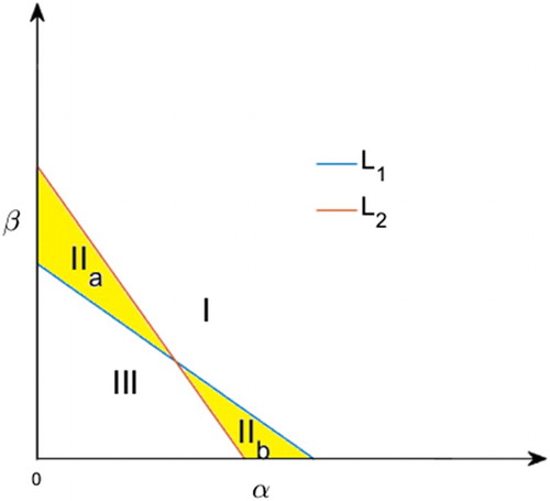
Define $\begin{array}{rl}{L}_1(\alpha ,\beta )& =a-\alpha -\frac{b}{c}\beta ,\\ L_2(\alpha ,\beta )& =d-\frac{f}{e}\alpha -\beta .\end{array}$ Then $L_1$ and $L_2$ divide the first quadrant of $\alpha ,\beta$ plane into at most four regions (see Figure 1).

Figure 1. Possible regions are separated by $L_i$ (i=1,2), in the $\alpha \beta$- plane.

Set $\begin{array}{rl}\mathrm{I}& :=\left\{\right(\alpha ,\beta ):L_i(\alpha ,\beta )<0,\alpha >0,\beta >0,i=1,2\},\\ \mathrm{II}& :=\left\{\right(\alpha ,\beta ):L_1(\alpha ,\beta \left)L_2\right(\alpha ,\beta )\le 0,\alpha >0,\beta >0\},\\ \mathrm{III}& :=\left\{\right(\alpha ,\beta ):L_i(\alpha ,\beta )>0,\alpha >0,\beta >0,i=1,2\}.\end{array}$ We are ready to state an important observation for system (1(1) $\begin{array}{rl}\frac{\mathrm{\partial }u}{\mathrm{\partial }t}& =d_1\mathrm{\Delta }u-\alpha u+\beta v+(a-bu-cv)u,\\ \frac{\mathrm{\partial }v}{\mathrm{\partial }t}& =d_2\mathrm{\Delta }v+\alpha u-\beta v+(d-eu-fv)v,\end{array}$(1) ) with the Neumann condition.

Proposition 2.5

Suppose $U(t,\cdot ,\mathrm{\Phi })=\left(u\right(t,\cdot ,\mathrm{\Phi }),v(t,\cdot ,\mathrm{\Phi }\left)\right)$ is the solution of system (1(1) $\begin{array}{rl}\frac{\mathrm{\partial }u}{\mathrm{\partial }t}& =d_1\mathrm{\Delta }u-\alpha u+\beta v+(a-bu-cv)u,\\ \frac{\mathrm{\partial }v}{\mathrm{\partial }t}& =d_2\mathrm{\Delta }v+\alpha u-\beta v+(d-eu-fv)v,\end{array}$(1) ) with Neumann boundary conditions and any bounded nonnegative initial data $\mathrm{\Phi }=({\phi }_1,{\phi }_2)$ with $\mathrm{\Phi }\not\equiv 0$. Then the following statements are valid.

1. If $(\alpha ,\beta )\in \mathrm{I},$ then system (1(1) $\begin{array}{rl}\frac{\mathrm{\partial }u}{\mathrm{\partial }t}& =d_1\mathrm{\Delta }u-\alpha u+\beta v+(a-bu-cv)u,\\ \frac{\mathrm{\partial }v}{\mathrm{\partial }t}& =d_2\mathrm{\Delta }v+\alpha u-\beta v+(d-eu-fv)v,\end{array}$(1) ) is cooperative in a positively invariant set $\mathcal{A}:=[0,\beta /c]\times [0,\alpha /e],$ and $U(t,\cdot ,\mathrm{\Phi })$ eventually lies in $[0,\beta /c)\times [0,\alpha /e);$

2. If $(\alpha ,\beta )\in \mathrm{III},$ then system (1(1) $\begin{array}{rl}\frac{\mathrm{\partial }u}{\mathrm{\partial }t}& =d_1\mathrm{\Delta }u-\alpha u+\beta v+(a-bu-cv)u,\\ \frac{\mathrm{\partial }v}{\mathrm{\partial }t}& =d_2\mathrm{\Delta }v+\alpha u-\beta v+(d-eu-fv)v,\end{array}$(1) ) is competitive in a positively invariant set $\mathcal{B}:=[\beta /c,(a-\alpha )/b]\times [\alpha /e,(d-\beta )/f],$ and $U(t,\cdot ,\mathrm{\Phi })$ eventually lies in $\mathrm{Int}\left(\mathcal{B}\right)$.

Proof.

For (a), in the system written in the form (2(2) $\begin{array}{rl}\frac{\mathrm{\partial }u}{\mathrm{\partial }t}& =d_1\mathrm{\Delta }u+g_1(u,v),\\ \frac{\mathrm{\partial }v}{\mathrm{\partial }t}& =d_2\mathrm{\Delta }v+g_2(u,v)\text{in}\mathrm{\Omega }\times (0,\mathrm{\infty }),\end{array}$(2) ), we have $g_1(\beta /c,v)=L_1(\alpha ,\beta )\beta /c<0$ and $g_2(u,\alpha /e)=L_2(\alpha ,\beta )\left(\alpha /e\right)<0$ for any $(u,v)\in \mathcal{A}$. Adapting the proof in Proposition 2.1, we obtain that (a) is valid.

For (b), it is easy to see that $g_1(\beta /c,v)=L_1(\alpha ,\beta )\left(\beta /c\right)>0,g_2(u,\alpha /e)=L_2(\alpha ,\beta )\left(\alpha /e\right)>0,$ $g_1((a-\alpha )/b,v)=(\beta -c((a-\alpha )/b\left)\right)v=-\left(c/b\right)L_1(\alpha ,\beta )v<0,$ and $g_2(u,(d-\beta )/f)=-\left(f/e\right)L_2(\alpha ,\beta )u<0$ for any $(u,v)\in \mathcal{B}$. Thus, $\mathcal{B}$ is contracting. Let $f_{-}(u,v)=(a-\alpha -bu)u-\left((d-\beta )/f\right)[cu-\beta {]}_{+}$ and $g_{-}(u,v)=(d-\beta -fv)v-\left((a-\alpha )/b\right)[ev-\alpha {]}_{+}$. Then $f_{-}(u,v)\le g_1(u,v)$ and $g_{-}(u,v)\le g_2(u,v)$ for $(u,v)\in \mathcal{B}$. Employing the same comparison argument as in Proposition 2.1, we can show that $\underset{t\to \mathrm{\infty }}{lim inf}u(t,\cdot ,\mathrm{\Phi })>\beta /c$ and $\underset{t\to \mathrm{\infty }}{lim inf}v(t,\cdot ,\mathrm{\Phi })>\alpha /e$.

Remark 2.6

Proposition 2.5 (a) is also valid for system (1(1) $\begin{array}{rl}\frac{\mathrm{\partial }u}{\mathrm{\partial }t}& =d_1\mathrm{\Delta }u-\alpha u+\beta v+(a-bu-cv)u,\\ \frac{\mathrm{\partial }v}{\mathrm{\partial }t}& =d_2\mathrm{\Delta }v+\alpha u-\beta v+(d-eu-fv)v,\end{array}$(1) ) under Dirichlet boundary conditions provided $a+d_1{\lambda }_d>0$ and $d+d_2{\lambda }_d>0$, and similarly for Robin conditions, based on analogous arguments in those cases.

2.4. Existence of positive equilibria with one component small

When $\alpha =\beta =0$, the system (1(1) $\begin{array}{rl}\frac{\mathrm{\partial }u}{\mathrm{\partial }t}& =d_1\mathrm{\Delta }u-\alpha u+\beta v+(a-bu-cv)u,\\ \frac{\mathrm{\partial }v}{\mathrm{\partial }t}& =d_2\mathrm{\Delta }v+\alpha u-\beta v+(d-eu-fv)v,\end{array}$(1) ) becomes a competitive Lotka–Volterra model. By standard results for diffusive logistic equations, as discussed for example in [9], Chapter 3, the system (1(1) $\begin{array}{rl}\frac{\mathrm{\partial }u}{\mathrm{\partial }t}& =d_1\mathrm{\Delta }u-\alpha u+\beta v+(a-bu-cv)u,\\ \frac{\mathrm{\partial }v}{\mathrm{\partial }t}& =d_2\mathrm{\Delta }v+\alpha u-\beta v+(d-eu-fv)v,\end{array}$(1) ) will have semi-trivial equilibria $(u_0,0)$ and $(0,v_0)$ in the boundary of the positive cone under Neumann boundary conditions if a>0 and d>0, and under Dirichlet boundary conditions if $a+d_1{\lambda }_d>0$ and $d+d_2{\lambda }_d>0$. We next look at the behaviour of boundary equilibria for $\alpha =\beta =0$ as those parameters become positive. For convenience, we only consider the Dirichlet boundary case. Other boundary conditions can be treated in a similar manner.

Lemma 2.7

Suppose $a+d_1{\lambda }_d>0$ $($respectively $d+d_2{\lambda }_d>0)$. If the semi-trivial steady state $(u_0,0)$ $($respectively $(0,v_0))$ is linearly stable when $\alpha =\beta =0,$ then it gives rise to a positive steady state $\left(u^{\ast }\right(\cdot ),v^{\ast }(\cdot \left)\right)$ close to $(u_0,0)$ $($respectively $(0,v_0))$ when α and β are sufficiently small.

Proof.

Here, we only consider the case, where $a+d_1{\lambda }_d>0$, the other case can be treated in a similar manner. Let $F:C_0^{2+\alpha }(\overline{\mathrm{\Omega }},\mathbb{R})\times C_0^{2+\alpha }(\overline{\mathrm{\Omega }},\mathbb{R})\times \mathbb{R}\to C^{\alpha }(\overline{\mathrm{\Omega }},{\mathbb{R}}^2)$ be defined by $F(u,v,z)=\left(\begin{array}{c}{d}_1\mathrm{\Delta }u-\alpha \left(z\right)u+\beta \left(z\right)v+(a-bu-cv)u\\ d_2\mathrm{\Delta }v+\alpha \left(z\right)u-\beta \left(z\right)v+(d-eu-fv)v\end{array}\right)$ where α and β are smooth, $\alpha \left(0\right)=\beta \left(0\right)=0$ and ${\alpha }^{\prime }\left(0\right)>0$, ${\beta }^{\prime }\left(0\right)>0$.

Clearly, the mapping F is continuous and differentiable. Indeed, we have (10) $D_{(u,v)}F(u,v,z)\left(\begin{array}{c}\phi \\ \psi \end{array}\right)=\left(\begin{array}{c}{d}_1\mathrm{\Delta }\phi +(a-\alpha -2bu-cv)\phi +(\beta -cu)\psi \\ d_2\mathrm{\Delta }\psi +(\alpha -ev)\phi +(d-\beta -eu-2fv)\psi \end{array}\right)$(10) It then follows that $F(u_0,0,0)=\left(\begin{array}{c}0\\ 0\end{array}\right)$ and (11) $D_{(u,v)}F(u_0,0,0)\left(\begin{array}{c}\phi \\ \psi \end{array}\right)=\left(\begin{array}{c}{d}_1\mathrm{\Delta }\phi +(a-2b{u}_0)\phi -c{u}_0\psi \\ d_2\mathrm{\Delta }\psi +(d-e{u}_0)\psi \end{array}\right)$(11) If 0 is not an eigenvalue of (12) $d_2\mathrm{\Delta }\psi +(d-e{u}_0)\psi =\sigma \psi \mathrm{in}\mathrm{\Omega },\psi =0\mathrm{on}\mathrm{\partial \Omega },$(12) then (13) $d_2\mathrm{\Delta }\psi +(d-e{u}_0)\psi =q,\mathrm{in}\mathrm{\Omega },\psi =0\mathrm{on}\mathrm{\partial \Omega }$(13) has a unique solution for any $q\in C^{\alpha }(\overline{\mathrm{\Omega }},\mathbb{R})$. Also, since $u_0>0$ in Ω, the principal eigenvalue for (14) $d_1\mathrm{\Delta }\rho +(a-b{u}_0)\rho =\tau \rho \mathrm{in}\mathrm{\Omega },\rho =0\mathrm{on}\mathrm{\partial \Omega }$(14) is $\tau =0$, so the principal eigenvalue of (15) $d_1\mathrm{\Delta }\rho +(a-2b{u}_0)\rho =\tau \rho \mathrm{in}\mathrm{\Omega },\rho =0\mathrm{on}\mathrm{\partial \Omega }$(15) will be negative. Therefore, if ψ is determined uniquely by Equation (13(13) $d_2\mathrm{\Delta }\psi +(d-e{u}_0)\psi =q,\mathrm{in}\mathrm{\Omega },\psi =0\mathrm{on}\mathrm{\partial \Omega }$(13) ) then the equation (16) $d_1\mathrm{\Delta }\phi +(a-2b{u}_0)\phi =p+c{u}_0\psi \mathrm{in}\mathrm{\Omega },\phi =0\mathrm{on}\mathrm{\partial \Omega }$(16) has a unique solution for any $p\in C^{\alpha }(\overline{\mathrm{\Omega }},\mathbb{R})$. This implies $D_{(u,v)}F(u_0,0,0)$ is invertible, and hence, it follows from the implicit function theorem that in some neighbourhood of $(u_0,0,0)$, the relation $F(u,v,z)=\left(\begin{array}{c}0\\ 0\end{array}\right)$ defines $u=u\left(z\right)$, $v=v\left(z\right)$ with u,v smooth in z. Consequently, we can differentiate $F(u,v,z)=\left(\begin{array}{c}0\\ 0\end{array}\right)$. $\begin{array}{rl}& d_1\mathrm{\Delta }{u}^{\prime }-{\alpha }^{\prime }u-\alpha u^{\prime }+{\beta }^{\prime }v+\beta v^{\prime }+(a-2bu-cv)u^{\prime }-cu{v}^{\prime }=0,\\ & d_2\mathrm{\Delta }{v}^{\prime }+{\alpha }^{\prime }u+\alpha u^{\prime }-{\beta }^{\prime }v-\beta v^{\prime }-ev{u}^{\prime }+(d-eu-2fv)v^{\prime }=0,\\ & u^{\prime }=v^{\prime }=0\mathrm{on}\mathrm{\partial \Omega }.\end{array}$ Evaluating the equation for $v^{\prime }$ at $(u_0,0,0)$ gives (17) $-d_2\mathrm{\Delta }{v}^{\prime }-(d-e{u}_0)v^{\prime }={\alpha }^{\prime }{u}_0>0\mathrm{in}\mathrm{\Omega }.$(17) When $(u_0,0)$ is linearly stable for system (1(1) $\begin{array}{rl}\frac{\mathrm{\partial }u}{\mathrm{\partial }t}& =d_1\mathrm{\Delta }u-\alpha u+\beta v+(a-bu-cv)u,\\ \frac{\mathrm{\partial }v}{\mathrm{\partial }t}& =d_2\mathrm{\Delta }v+\alpha u-\beta v+(d-eu-fv)v,\end{array}$(1) ), the principal eigenvalue for Equation (12(12) $d_2\mathrm{\Delta }\psi +(d-e{u}_0)\psi =\sigma \psi \mathrm{in}\mathrm{\Omega },\psi =0\mathrm{on}\mathrm{\partial \Omega },$(12) ) is negative, so the principal eigenvalue and hence all other eigenvalues of (18) $L\psi :=-d_2\mathrm{\Delta }\psi -(d-e{u}_0)\psi =\gamma \psi \mathrm{in}\mathrm{\Omega },\psi =0\mathrm{on}\mathrm{\partial \Omega }$(18) are positive, so the operator L has a positive resolvent (in other words, Equation (17(17) $-d_2\mathrm{\Delta }{v}^{\prime }-(d-e{u}_0)v^{\prime }={\alpha }^{\prime }{u}_0>0\mathrm{in}\mathrm{\Omega }.$(17) ) has a maximum principle) which implies that $v^{\prime }>0$ in Ω. Thus, increasing z slightly from z=0 will produce a positive steady state $(u_0^{\ast },v_0^{\ast })$ with both components positive in Ω. In other words, if $(\alpha ,\beta )$ are small enough, there is a positive steady state close to $(u_0,0)$. The argument in the case of $(0,v_0)$ is analogous to that for $(u_0,0)$.

3. Spatially homogeneous case

To better understand the effect of the switching rates α and β on the dynamics of the system (1(1) $\begin{array}{rl}\frac{\mathrm{\partial }u}{\mathrm{\partial }t}& =d_1\mathrm{\Delta }u-\alpha u+\beta v+(a-bu-cv)u,\\ \frac{\mathrm{\partial }v}{\mathrm{\partial }t}& =d_2\mathrm{\Delta }v+\alpha u-\beta v+(d-eu-fv)v,\end{array}$(1) ), we first study the ODE system (19) $\begin{array}{rl}\frac{\mathrm{d}u}{\mathrm{d}t}& =-\alpha u+\beta v+(a-bu-cv)u,\\ \frac{\mathrm{d}v}{\mathrm{d}t}& =\alpha u-\beta v+(d-eu-fv)v.\end{array}$(19) In view of Proposition 2.2, it follows that $(0,0)$ is unstable. Next, we discuss the existence and stability of positive equilibria.

3.1. Basic properties of equilibria

Let $(u^{\ast },v^{\ast })$ be a positive equilibrium of system (19(19) $\begin{array}{rl}\frac{\mathrm{d}u}{\mathrm{d}t}& =-\alpha u+\beta v+(a-bu-cv)u,\\ \frac{\mathrm{d}v}{\mathrm{d}t}& =\alpha u-\beta v+(d-eu-fv)v.\end{array}$(19) ). Then we have (20) $\begin{array}{rl}-\alpha u^{\ast }+\beta v^{\ast }+(a-b{u}^{\ast }-c{v}^{\ast })u^{\ast }& =0,\\ \alpha u^{\ast }-\beta v^{\ast }+(d-e{u}^{\ast }-f{v}^{\ast })v^{\ast }& =0.\end{array}$(20) Set $k=v^{\ast }/u^{\ast }$. Substitute k into system (20(20) $\begin{array}{rl}-\alpha u^{\ast }+\beta v^{\ast }+(a-b{u}^{\ast }-c{v}^{\ast })u^{\ast }& =0,\\ \alpha u^{\ast }-\beta v^{\ast }+(d-e{u}^{\ast }-f{v}^{\ast })v^{\ast }& =0.\end{array}$(20) ) and simplify the equations. We get (21) $u^{\ast }=\frac{a-\alpha +\beta k}{b+ck}=\frac{\alpha k^{-1}+d-\beta }{e+fk}.$(21) Note that if $k\in (0,\alpha /\beta )$, it follows from $\alpha k^{-1}+d-\beta >0$ that $u^{\ast }>0$, and if $k\in [\alpha /\beta ,\mathrm{\infty })$, then we have $u^{\ast }>0$ because of $a-\alpha +\beta k>0$. Thus, it suffices to find the positive values of k satisfying the equation $\frac{a-\alpha +\beta k}{b+ck}=\frac{\alpha k^{-1}+d-\beta }{e+fk}.$ Simplifying the above formula, we get the cubic equation: (22) $\begin{array}{rl}P\left(k\right)& :=\beta f{k}^3+\left[\right((a-\alpha )f+\beta e-c(d-\beta )\left)\right]k^2\\ & +\left[\right(a-\alpha )e-\alpha c-(d-\beta \left)b\right]k-\alpha b=0.\end{array}$(22) Since $P\left(0\right)=-\alpha b<0$ and $P\left(\mathrm{\infty }\right)=\mathrm{\infty }$, we immediately obtain that there exists at least one positive root $k^{\ast }$ for $P\left(k\right)$.

Therefore, system (19(19) $\begin{array}{rl}\frac{\mathrm{d}u}{\mathrm{d}t}& =-\alpha u+\beta v+(a-bu-cv)u,\\ \frac{\mathrm{d}v}{\mathrm{d}t}& =\alpha u-\beta v+(d-eu-fv)v.\end{array}$(19) ) admits (at least) one positive equilibrium $(u^{\ast },v^{\ast })$, and at most three positive equilibria.

Proposition 3.1

Suppose $(u^{\ast },v^{\ast })$ is any positive equilibrium for system (19(19) $\begin{array}{rl}\frac{\mathrm{d}u}{\mathrm{d}t}& =-\alpha u+\beta v+(a-bu-cv)u,\\ \frac{\mathrm{d}v}{\mathrm{d}t}& =\alpha u-\beta v+(d-eu-fv)v.\end{array}$(19) ).

1. If $L_1(\alpha ,\beta )L_2(\alpha ,\beta )>0$ and $(u^{\ast },v^{\ast })$ is hyperbolic, then it is either a saddle or a stable node. Moreover, it is always a stable node provided $bf\ge ce$.

2. If $L_1(\alpha ,\beta )L_2(\alpha ,\beta )\le 0,$ then $(u^{\ast },v^{\ast })$ is hyperbolic and could be a stable node or stable spiral.

Proof.

Consider the Jacobian matrix at $(u^{\ast },v^{\ast })$, namely $J(u^{\ast },v^{\ast })=\left(\begin{array}{cc}a-\alpha -2b{u}^{\ast }-c{v}^{\ast }& \beta -c{u}^{\ast }\\ \alpha -e{v}^{\ast }& d-\beta -2f{v}^{\ast }-e{u}^{\ast }\end{array}\right).$ Note that $a-\alpha -b{u}^{\ast }-c{v}^{\ast }+\beta \left(v^{\ast }/u^{\ast }\right)=0$ and $d-\beta -f{v}^{\ast }-e{u}^{\ast }+\alpha \left(u^{\ast }/v^{\ast }\right)=0$. Thus, we have $J(u^{\ast },v^{\ast })=\left(\begin{array}{cc}-b{u}^{\ast }-\beta \frac{v^{\ast }}{u^{\ast }}& \beta -c{u}^{\ast }\\ \alpha -e{v}^{\ast }& -f{v}^{\ast }-\alpha \frac{u^{\ast }}{v^{\ast }}\end{array}\right)=\left(\begin{array}{cc}{a}_{11}& a_{12}\\ a_{21}& a_{22}\end{array}\right),$ where $a_{11}=-b{u}^{\ast }-\beta \left(v^{\ast }/u^{\ast }\right)<0$, $a_{22}=-f{v}^{\ast }-\alpha \left(u^{\ast }/v^{\ast }\right)<0$, $a_{12}=\beta -c{u}^{\ast }$ and $a_{21}=\alpha -e{v}^{\ast }$. We have (23) $det\left(J\right)=a_{11}{a}_{22}-a_{12}{a}_{21}=(bf-ce)u^{\ast }{v}^{\ast }+\beta f\frac{v^{\ast 2}}{u^{\ast }}+\alpha b\frac{u^{\ast 2}}{v^{\ast }}+e\beta v^{\ast }+\alpha c{u}^{\ast },$(23) $\mathrm{tr}\left(J\right)=a_{11}+a_{22}<0$, and $\left(\mathrm{tr}\right(J){)}^2-4det(J)=(a_{11}+a_{22}{)}^2-4(a_{11}{a}_{22}-a_{12}{a}_{21})=(a_{11}-a_{22}{)}^2+4a_{12}{a}_{21}.$

In the case where $L_1(\alpha ,\beta )L_2(\alpha ,\beta )>0$, it follows from Proposition 2.5 that $a_{12}{a}_{21}>0$, and hence, $\left(\mathrm{tr}\right(J){)}^2-4det(J)>0$. If $detJ\ne 0$, $(u^{\ast },v^{\ast })$ is either a saddle or a stable node. Moreover, it easily follows that if $bf-ce\ge 0$, then $detJ>0$ and $(u^{\ast },v^{\ast })$ is always a stable node. In the case where $L_1(\alpha ,\beta )L_2(\alpha ,\beta )\le 0$, suppose $L_1(\alpha ,\beta )\ge 0$ and $L_2(\alpha ,\beta )\le 0$.(The other case is similar.) Note that $u^{\ast }>\beta /c$ and $v^{\ast }>\alpha /e$ are equivalent to $L_1(\alpha ,\beta )>0$ and $L_2(\alpha ,\beta )>0$, respectively. Indeed, If $u^{\ast }>\beta /c$, then $L_1(\alpha ,\beta )>a-\alpha -b{u}^{\ast }=\left(v^{\ast }/u^{\ast }\right)(c{u}^{\ast }-\beta )>0$. Meanwhile, if $u^{\ast }\le \beta /c$, then $L_1(\alpha ,\beta )\le a-\alpha -b{u}^{\ast }=\left(v^{\ast }/u^{\ast }\right)(c{u}^{\ast }-\beta )\le 0$. Now $L_1(\alpha ,\beta )\ge 0$ and $L_2(\alpha ,\beta )\le 0$ yield $u^{\ast }\ge \beta /c$ and $v^{\ast }\le \alpha /e$, that is, $a_{12}{a}_{21}\le 0$. It then follows that $detJ=a_{11}{a}_{22}-a_{12}{a}_{21}\ge a_{11}{a}_{22}>0$, and hence, the equilibrium is hyperbolic. However, it is not obvious that what type of equilibrium it is. Indeed, numerical computation indicates that $(u^{\ast },v^{\ast })$ could be a stable node or stable spiral.

3.2. Conditions for global stability

Next, we use a Lyapunov function to prove the global stability of the positive equilibrium $(u^{\ast },v^{\ast })$ for α and β in certain regions of the $\alpha \beta$-plane. This analysis will also extend to the PDE case with Neumann boundary conditions, which we will discuss later. Let $F_1\left(u\right)=u-u^{\ast }-u^{\ast }\ln \left(u/u^{\ast }\right)$ and $F_2\left(v\right)=v-v^{\ast }-v^{\ast }\ln \left(v/v^{\ast }\right)$.

Lemma 3.2

1. If $(\alpha ,\beta )\in \mathrm{II},$ then there exists $c_i>0,i=1,2,$ such that $V=c_1{F}_1+c_2{F}_2$ satisfies $\mathrm{d}V/\mathrm{d}t\le 0$ along any positive solution $(u,v)$ of system (19(19) $\begin{array}{rl}\frac{\mathrm{d}u}{\mathrm{d}t}& =-\alpha u+\beta v+(a-bu-cv)u,\\ \frac{\mathrm{d}v}{\mathrm{d}t}& =\alpha u-\beta v+(d-eu-fv)v.\end{array}$(19) ). The equality holds if and only if $(u,v)\equiv (u^{\ast },v^{\ast })$.

2. If $(\alpha ,\beta )\in III$ and $bf>(c-\beta /u^{\ast })(e-\alpha /v^{\ast }),$ then there exists $c_i>0,i=1,2,$ such that $V=c_1{F}_1+c_2{F}_2$ satisfies $\mathrm{d}V/\mathrm{d}t\le 0$ along any positive solution $(u,v)$ of system (19(19) $\begin{array}{rl}\frac{\mathrm{d}u}{\mathrm{d}t}& =-\alpha u+\beta v+(a-bu-cv)u,\\ \frac{\mathrm{d}v}{\mathrm{d}t}& =\alpha u-\beta v+(d-eu-fv)v.\end{array}$(19) ). The equality holds if and only if $(u,v)\equiv (u^{\ast },v^{\ast })$.

Proof.

For the sake of illustration, we refer to Figure 1. If $(\alpha ,\beta )\in \mathrm{II}$, then $(\alpha ,\beta )\in {\mathrm{II}}_a$ or ${\mathrm{II}}_b$ including the interior boundary. By the proofs of Proposition 3.1(b) and Proposition 2.5, it follows that $(u^{\ast }-\beta /c)(v^{\ast }-\alpha /e)\le 0$ if and only if $(\alpha ,\beta )\in \mathrm{II}$, $u^{\ast }>\beta /c$ and $v^{\ast }>\alpha /e$ if and only if $(\alpha ,\beta )\in \mathrm{III}$. Furthermore, $\begin{array}{rl}\frac{\mathrm{d}{F}_1}{\mathrm{d}t}& =\left(1-\frac{u^{\ast }}{u}\right)\frac{\mathrm{d}u}{\mathrm{d}t}=(u-u^{\ast })\left(-\alpha +\beta \frac{v}{u}+a-bu-cv\right)\\ & =(u-u^{\ast })\left[-b(u-u^{\ast })-c(v-v^{\ast })+\beta \left(\frac{v}{u}-\frac{v^{\ast }}{u^{\ast }}\right)\right]\\ & =-b(u-u^{\ast }{)}^2-c(u-u^{\ast }\left)\right(v-v^{\ast })+\beta (u-u^{\ast })\left(\frac{v}{u}-\frac{v^{\ast }}{u^{\ast }}\right)\\ & \le -b(u-u^{\ast }{)}^2-\left(c-\frac{\beta }{u^{\ast }}\right)(u-u^{\ast }\left)\right(v-v^{\ast })\\ & =-b(u-u^{\ast }{)}^2-\frac{c}{u^{\ast }}(u^{\ast }-\frac{\beta }{c}\left)\right(u-u^{\ast }\left)\right(v-v^{\ast }).\end{array}$ The inequality above is valid since if $u\left(t_0\right)>u^{\ast }>0$ for some $t_0\ge 0$, then $v/u-v^{\ast }/u^{\ast }\le (v-v^{\ast })/u^{\ast }$, and hence $\beta (u-u^{\ast })(v/u-v^{\ast }/u^{\ast })\le \left(\beta /u^{\ast }\right)(u-u^{\ast })(v-v^{\ast })$. On the other hand, if $u^{\ast }>u\left(t_0\right)>0$ for some $t_0\ge 0$, then we have $v/u-v^{\ast }/u^{\ast }\ge (v-v^{\ast })/u^{\ast }$ and $u-u^{\ast }<0$, and hence, we still have $\beta (u-u^{\ast })(v/u-v^{\ast }/u^{\ast })\le \left(\beta /u^{\ast }\right)(u-u^{\ast })(v-v^{\ast })$. In other words, we always have $\beta (u-u^{\ast })(v/u-v^{\ast }/u^{\ast })\le \left(\beta /u^{\ast }\right)(u-u^{\ast })(v-v^{\ast })$.

Similarly, we also have $\frac{\mathrm{d}{F}_2}{\mathrm{d}t}\le -f(v-v^{\ast }{)}^2-\frac{e}{v^{\ast }}\left(v^{\ast }-\frac{\alpha }{e}\right)(u-u^{\ast }\left)\right(v-v^{\ast }).$ Note that if AD>BC and A,D are positive, then there exists K>0 such that $A{x}^2+Bxy+K(Cxy+D{y}^2)>0,$ for every $x\ge 0,y\ge 0$ except $(0,0)$.

Clearly, $\begin{array}{rl}& A{x}^2+(B+CK)xy+DK{y}^2=A{\left(x+\frac{B+CK}{2A}y\right)}^2\\ & +\left(-\frac{B^2}{4A}+DK-\frac{BC}{2A}K-\frac{C^2}{4A}{K}^2\right)y^2\end{array}$ stays positive for every $x\ge 0,y\ge 0$ except $(0,0)$ provided we can choose K>0 so that $-\frac{B^2}{4A}+\left(D-\frac{BC}{2A}\right)K-\frac{C^2}{4A}{K}^2>0.$ Such is the case if the discriminant Δ for $-B^2/4A+(D-BC/2A)K-\left(C^2/4A\right)K^2=0$ is positive. Since $\mathrm{\Delta }={\left(D-\frac{BC}{2A}\right)}^2-\frac{B^2{C}^2}{4A^2}=D^2-\frac{DBC}{A}>0,$ the result follows.

Now let A=b, D=f, $B=c-\beta /u^{\ast }$ and $C=e-\alpha /v^{\ast }$. In region ${\mathrm{II}}_a$, ${\mathrm{II}}_b$, it is easy to see that $BC\le 0<AD$, and hence, there exists $K_1>0$ such that for $V=F_1+K_1{F}_2$ we have $\frac{\mathrm{d}V}{\mathrm{d}t}\le 0.$ The equality holds true if and only if $(u,v)\equiv (u^{\ast },v^{\ast })$.

In Region III, B and C are positive, we need AD>BC, that is, $bf>(c-\beta /u^{\ast })(e-\alpha /v^{\ast })$. Then there exists $K_2>0$ such that for $V=F_1+K_2{F}_2$ we have $\frac{\mathrm{d}V}{\mathrm{d}t}\le 0.$ The equality holds true if and only if $(u,v)\equiv (u^{\ast },v^{\ast })$.

Remark 3.3

If $(\alpha ,\beta )\in \mathrm{III}$ and $bf\ge ce$, e.g. in the weak competition case ($b/e>a/d>c/f$, a unique stable coexistence), the condition in part (b) is automatically valid because $bf\ge ce>\left(c-\frac{\beta }{u^{\ast }}\right)\left(e-\frac{\alpha }{v^{\ast }}\right).$

3.3. Bifurcations

Next, we will explore some bifurcations for the system (19(19) $\begin{array}{rl}\frac{\mathrm{d}u}{\mathrm{d}t}& =-\alpha u+\beta v+(a-bu-cv)u,\\ \frac{\mathrm{d}v}{\mathrm{d}t}& =\alpha u-\beta v+(d-eu-fv)v.\end{array}$(19) ). Consider the strong competition case, that is, bf<ce. First, we give the number of positive equilibria when α and β are small enough.

Proposition 3.4

Suppose bf<ce. If $c/f>a/d>b/e,$ then system (19(19) $\begin{array}{rl}\frac{\mathrm{d}u}{\mathrm{d}t}& =-\alpha u+\beta v+(a-bu-cv)u,\\ \frac{\mathrm{d}v}{\mathrm{d}t}& =\alpha u-\beta v+(d-eu-fv)v.\end{array}$(19) ) has three positive equilibria when $(\alpha ,\beta )$ are small enough. If either $a/d>c/f>b/e$ or $c/f>b/e>a/d$ holds, then system (19(19) $\begin{array}{rl}\frac{\mathrm{d}u}{\mathrm{d}t}& =-\alpha u+\beta v+(a-bu-cv)u,\\ \frac{\mathrm{d}v}{\mathrm{d}t}& =\alpha u-\beta v+(d-eu-fv)v.\end{array}$(19) ) has a unique positive equilibrium when $(\alpha ,\beta )$ are small enough.

Proof.

The proof is based on using the cubic discriminant and checking the signs of coefficients in Equation (22(22) $\begin{array}{rl}P\left(k\right)& :=\beta f{k}^3+\left[\right((a-\alpha )f+\beta e-c(d-\beta )\left)\right]k^2\\ & +\left[\right(a-\alpha )e-\alpha c-(d-\beta \left)b\right]k-\alpha b=0.\end{array}$(22) ). Recall that the discriminant of the cubic $A{x}^3+B{x}^2+Cx+D$ is $B^2{C}^2-4A{C}^3-4B^{3}D-27A^2{D}^2+18ABCD$, and that when it is positive the cubic has three distinct real roots. For the polynomial $P\left(k\right)$ all terms in the discriminant except the one corresponding to $B^2{C}^2$ go to zero as α and β go to zero, and when $a/d\ne c/f$ and $a/d\ne b/e$ the limit of the remaining term is positive, so when $\alpha ,\beta$ are small enough $P\left(k\right)$ always has three distinct real roots $k_i(i=1,2,3)$. Now when $c/f>a/d>b/e$ and $\alpha =\beta =0$, system (19(19) $\begin{array}{rl}\frac{\mathrm{d}u}{\mathrm{d}t}& =-\alpha u+\beta v+(a-bu-cv)u,\\ \frac{\mathrm{d}v}{\mathrm{d}t}& =\alpha u-\beta v+(d-eu-fv)v.\end{array}$(19) ) admits two linearly stable boundary equilibria. Adapting the proof in Lemma 2.7, together with the fact $k_1{k}_2{k}_3=\alpha b/\beta f>0$, we see that system (19(19) $\begin{array}{rl}\frac{\mathrm{d}u}{\mathrm{d}t}& =-\alpha u+\beta v+(a-bu-cv)u,\\ \frac{\mathrm{d}v}{\mathrm{d}t}& =\alpha u-\beta v+(d-eu-fv)v.\end{array}$(19) ) admits three positive equilibria. When α, β are small enough and $a/d>c/f>b/e$ (or $c/f>b/e>a/d$) holds, we have $k_1+k_2+k_3=-(af-cd-f\alpha +(c+e\left)\beta \right)/\beta f<0$ (or $k_1{k}_2+k_1{k}_3+k_2{k}_3=(ae-bd-(c+e)\alpha +b\beta )/\beta f<0$). Since $k_1{k}_2{k}_3>0$ is positive, we see system (19(19) $\begin{array}{rl}\frac{\mathrm{d}u}{\mathrm{d}t}& =-\alpha u+\beta v+(a-bu-cv)u,\\ \frac{\mathrm{d}v}{\mathrm{d}t}& =\alpha u-\beta v+(d-eu-fv)v.\end{array}$(19) ) has a unique positive equilibrium.

Now we are ready to introduce the main result on the bifurcation of system (19(19) $\begin{array}{rl}\frac{\mathrm{d}u}{\mathrm{d}t}& =-\alpha u+\beta v+(a-bu-cv)u,\\ \frac{\mathrm{d}v}{\mathrm{d}t}& =\alpha u-\beta v+(d-eu-fv)v.\end{array}$(19) ).

Theorem 3.5

Suppose $bf<ce,$ then a $($codimension-two$)$ cusp bifurcation occurs at the bifurcation curve in the $\alpha \beta$-plane with parametric form (24) $\begin{array}{rl}\alpha & =\frac{k^2[mf{k}^2+2nfk+n(e+c)-mb]}{[f{k}^2+(e+c)k+b{]}^2},\\ \beta & =\frac{[fn-m(e+c\left)\right]k^2-2mbk-nb}{[f{k}^2+(e+c)k+b{]}^2},\end{array}$(24) where m=af−cd and $n=ae-bd,$ and k satisfies one of the following cases:

1. If $c/f>a/d>b/e,$ that is, $m<0,n>0,$ then $k\in [k_1^{\ast },k_2^{\ast }]$, where $k_1^{\ast }$ and $k_2^{\ast }$ are the unique positive roots of Equations (26(26) $[fn-m(e+c\left)\right]k^2-2mbk-nb=0.$(26) ) and (29(29) $mf{k}^2+2nfk+n(e+c)-mb=0.$(29) ) $($shown below$),$ respectively.

2. If $a/d\ge c/f>b/e,$ that is, $m\ge 0,$ $n>0,$ and $fn-m(e+c)>0,$ then $k\in [k_1^{\ast },\mathrm{\infty })$.

3. If $c/f>b/e\ge a/d,$ that is, $m<0,$ $n\le 0,$ and $n(e+c)-mb>0,$ then $k\in (0,k_2^{\ast }]$.

Moreover, any non-hyperbolic equilibrium only occurs when $(\alpha ,\beta )$ lies on the bifurcation curve (24(24) $\begin{array}{rl}\alpha & =\frac{k^2[mf{k}^2+2nfk+n(e+c)-mb]}{[f{k}^2+(e+c)k+b{]}^2},\\ \beta & =\frac{[fn-m(e+c\left)\right]k^2-2mbk-nb}{[f{k}^2+(e+c)k+b{]}^2},\end{array}$(24) ) provided one of (A1)–(A3) holds.

Proof.

(A1) Bistable case ($c/f>a/d>b/e$): when $\alpha =\beta =0$, the system (19(19) $\begin{array}{rl}\frac{\mathrm{d}u}{\mathrm{d}t}& =-\alpha u+\beta v+(a-bu-cv)u,\\ \frac{\mathrm{d}v}{\mathrm{d}t}& =\alpha u-\beta v+(d-eu-fv)v.\end{array}$(19) ) has two stable boundary equilibrium points and one unstable positive equilibrium point. The cubic equation is $\beta f{k}^3+[m-\alpha f+(e+c\left)\beta \right]k^2+[n-(c+e)\alpha +b\beta ]k-\alpha b=0$. Rewrite the equation as follows: $m{k}^2+nk=-(\beta k-\alpha )[f{k}^2+(e+c)k+b].$ Note that for any $k\ge 0$, $f{k}^2+(e+c)k+b>0$, thus we have (25) $V\left(k\right):=\frac{m{k}^2+nk}{f{k}^2+(e+c)k+b}=\alpha -\beta k.$(25)

The left-hand-side of Equation (25(25) $V\left(k\right):=\frac{m{k}^2+nk}{f{k}^2+(e+c)k+b}=\alpha -\beta k.$(25) ) represents a curve which is fixed, independent of α and β, and the right-hand side gives a line with two parameters. Moreover, $\begin{array}{rl}{V}^{\prime }\left(k\right)& =\frac{(2mk+n)[f{k}^2+(e+c)k+b]-(m{k}^2+nk)(2fk+e+c)}{[f{k}^2+(e+c)k+b{]}^2}\\ & =-\frac{[fn-m(e+c\left)\right]k^2-2mbk-nb}{[f{k}^2+(e+c)k+b{]}^2}\end{array}$ Since m<0 and n>0, it follows that $fn-m(e+c)>0$. Let $k_1^{\ast }$ be the positive root of (26) $[fn-m(e+c\left)\right]k^2-2mbk-nb=0.$(26) For $k\in (0,k_1^{\ast })$, $V^{\prime }\left(k\right)>0$, and for $k\in (k_1^{\ast },\mathrm{\infty })$, $V^{\prime }\left(k\right)<0$, and $V\left(0\right)=0$, $V\left(\mathrm{\infty }\right)=m/f<0$. This will help to plot the curve $V\left(k\right)$. Note that as α and β vary, the line on the right-hand side of Equation (25(25) $V\left(k\right):=\frac{m{k}^2+nk}{f{k}^2+(e+c)k+b}=\alpha -\beta k.$(25) ) moves but the curve does not. This suggests that analysing the intersections of the curve and the line graphically should be possible. The essential arguments used to find the number of intersections of two curves are similar to those in the Spruce Budworm model [28].

For example, fix a sufficiently small α, let β increase (or fix a relatively large α, let β increase), then the line rotates clockwise around $(0,\alpha )$. Now we have the following pictures.

We need to find the bifurcation turning point. This requires us to check the tangency condition. Taking the derivative (with respect to k) for both sides of Equation (25(25) $V\left(k\right):=\frac{m{k}^2+nk}{f{k}^2+(e+c)k+b}=\alpha -\beta k.$(25) ), we have (27) $\beta =-V^{\prime }\left(k\right)=\frac{[fn-m(e+c\left)\right]k^2-2mbk-nb}{[f{k}^2+(e+c)k+b{]}^2}.$(27) So for any $k>k_1^{\ast }$, we have $\beta >0$.

On the other hand, we have (28) $\alpha =k\left(\beta +\frac{mk+n}{f{k}^2+(e+c)k+b}\right)=\frac{k^2[mf{k}^2+2nfk+n(e+c)-mb]}{[f{k}^2+(e+c\left)k\right]+b{]}^2}.$(28) Note that mf<0 and $n(e+c)-mb>0$. Let $k_2^{\ast }$ be the positive root of equation (29) $mf{k}^2+2nfk+n(e+c)-mb=0.$(29) Then $k_2^{\ast }>-n/m>0$. Actually, we have $k_1^{\ast }<-n/m$. Let $G\left(k\right)=[fn-m(e+c\left)\right]k^2-2mbk-nb$. We just need check $G(-n/m)>0$. Indeed, $G\left(-\frac{n}{m}\right)=[fn-m(e+c\left)\right]\frac{n^2}{m^2}+2bn-nb=n\left[f{\left(\frac{n}{m}\right)}^2-(e+c)\frac{n}{m}+b\right]>0.$ In a word, we have (30) $\begin{array}{rl}\alpha & =\frac{k^2[mf{k}^2+2nfk+n(e+c)-mb]}{[f{k}^2+(e+c)k+b{]}^2}\end{array}$(30) (31) $\begin{array}{rl}\beta & =\frac{[fn-m(e+c\left)\right]k^2-2mbk-nb}{[f{k}^2+(e+c)k+b{]}^2}\end{array}$(31) where $k\in [k_1^{\ast },k_2^{\ast }]$.

Checking the derivatives of $\alpha \left(k\right)$ and $\beta \left(k\right)$ with respect to k, we have ${\alpha }^{\prime }\left(k\right)=-k{V}^{″}\left(k\right)$, ${\beta }^{\prime }\left(k\right)=-V^{″}\left(k\right)$ and $-V^{″}\left(k\right)=\frac{-2f[fn-m(e+c\left)\right]k^3+6mbf{k}^2+6fnbk-2m{b}^2+2(e+c)nb}{[f{k}^2+(e+c)k+b{]}^3}.$ Since n>0 and m<0, it is easy to see that there exists a unique $k_c>0$ such that $V^{″}\left(k\right)=0$. Therefore, $\left(\alpha \right(k_c),\beta (k_c\left)\right)$ is the cusp point with ${\alpha }^{\prime }\left(k_c\right)={\beta }^{\prime }\left(k_c\right)=0$. Moreover, $\alpha \left(k\right)$ and $\beta \left(k\right)$ are increasing on $(k_1^{\ast },k_c)$ and decreasing on $(k_c,k_2^{\ast })$. See Figure 3. In a word, a typical cusp bifurcation occurs.

Figure 2. The left panel indicates when β is small, there are three intersections, then increasing β, finally, there will be only one intersection. The right panel shows that when β is small, there is only one intersection, then as β gets bigger, the number of intersection will be $1\to 2\to 3\to 2\to 1$.

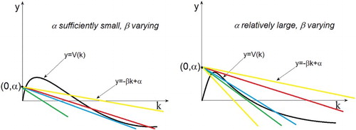
Figure 3. Inside the curve, there are three distinct positive fixed points, on the curve, there are two fixed points, outside the curve there is one. This is for the bistable case.

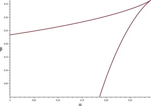
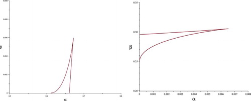
In the competitive exclusion case (A2) or (A3), see Figure 4 for illustration. We have

Figure 4. The left curve for case (A2) intersects α-axis at $(m/f,0)$ and $((m{k}_1^{\ast 2}+n{k}_1^{\ast })/(f{k}_1^{\ast 2}+(e+c)k_1^{\ast }+b),0)$. Inside the curve, there are three distinct positive fixed points, on the curve, two fixed points, and outside, one. The right curve for case (A3) intersects $\beta$-axis at $(0,-n/b)$ and $(0,-(m{k}_2^{\ast }+n)/(f{k}_2^{\ast 2}+(e+c)k_2^{\ast }+b))$. Inside the curve, there are three distinct positive fixed points, on the curve, two fixed points, and outside, one.

(A2) $m\ge 0,n>0$ and ce>bf.

Now, mimicking our previous analysis, we have (32) $\begin{array}{rl}\alpha & =\frac{k^2[mf{k}^2+2nfk+n(e+c)-mb]}{[f{k}^2+(e+c)k+b{]}^2}\\ \beta & =\frac{[fn-m(e+c\left)\right]k^2-2mbk-nb}{[f{k}^2+(e+c)k+b{]}^2}\end{array}$(32) Since $m\ge 0$, n>0, a necessary condition for $\beta \ge 0$ in Equation (32(32) $\begin{array}{rl}\alpha & =\frac{k^2[mf{k}^2+2nfk+n(e+c)-mb]}{[f{k}^2+(e+c)k+b{]}^2}\\ \beta & =\frac{[fn-m(e+c\left)\right]k^2-2mbk-nb}{[f{k}^2+(e+c)k+b{]}^2}\end{array}$(32) ) is $fn-m(e+c)>0$. If $fn-m(e+c)\le 0$, then $V^{\prime }\left(k\right)>0$ for $k\in \mathbb{R}$. It then follows that Equation (25(25) $V\left(k\right):=\frac{m{k}^2+nk}{f{k}^2+(e+c)k+b}=\alpha -\beta k.$(25) ) has only one root, and hence, system (19(19) $\begin{array}{rl}\frac{\mathrm{d}u}{\mathrm{d}t}& =-\alpha u+\beta v+(a-bu-cv)u,\\ \frac{\mathrm{d}v}{\mathrm{d}t}& =\alpha u-\beta v+(d-eu-fv)v.\end{array}$(19) ) admits a unique positive equilibrium. Since $n/m>(e+c)/f>b/(e+c)$, it follows that $mf{k}^2+2nfk+n(e+c)-mb>0$ for $k\ge 0$. Now if $k>k_1^{\ast }$, we have $\beta >0$ and $\alpha >0$ in Equation (32(32) $\begin{array}{rl}\alpha & =\frac{k^2[mf{k}^2+2nfk+n(e+c)-mb]}{[f{k}^2+(e+c)k+b{]}^2}\\ \beta & =\frac{[fn-m(e+c\left)\right]k^2-2mbk-nb}{[f{k}^2+(e+c)k+b{]}^2}\end{array}$(32) ).

(A3) $m<0,n\le 0$ and ce>bf.

The tangency condition will also give the same parametric form as Equation (32(32) $\begin{array}{rl}\alpha & =\frac{k^2[mf{k}^2+2nfk+n(e+c)-mb]}{[f{k}^2+(e+c)k+b{]}^2}\\ \beta & =\frac{[fn-m(e+c\left)\right]k^2-2mbk-nb}{[f{k}^2+(e+c)k+b{]}^2}\end{array}$(32) ). Note that $fn-m(e+c)=(ae-bd)f-(af-cd)(e+c)=-cm+d(ce-bf)>0$. It follows that $[fn-m(e+c\left)\right]k^2-2mbk-nb>0$ for any k>0. Thus, $\beta >0$ in Equation (32(32) $\begin{array}{rl}\alpha & =\frac{k^2[mf{k}^2+2nfk+n(e+c)-mb]}{[f{k}^2+(e+c)k+b{]}^2}\\ \beta & =\frac{[fn-m(e+c\left)\right]k^2-2mbk-nb}{[f{k}^2+(e+c)k+b{]}^2}\end{array}$(32) ) for any k>0. If $n(e+c)-mb\le 0$, then for any k>0, $\alpha <0$ in Equation (32(32) $\begin{array}{rl}\alpha & =\frac{k^2[mf{k}^2+2nfk+n(e+c)-mb]}{[f{k}^2+(e+c)k+b{]}^2}\\ \beta & =\frac{[fn-m(e+c\left)\right]k^2-2mbk-nb}{[f{k}^2+(e+c)k+b{]}^2}\end{array}$(32) ). Thus it is necessary that $n(e+c)-mb>0$; that is, $ce-bf>-ne/a\ge 0$. This leads to $\alpha >0$ in Equation (32(32) $\begin{array}{rl}\alpha & =\frac{k^2[mf{k}^2+2nfk+n(e+c)-mb]}{[f{k}^2+(e+c)k+b{]}^2}\\ \beta & =\frac{[fn-m(e+c\left)\right]k^2-2mbk-nb}{[f{k}^2+(e+c)k+b{]}^2}\end{array}$(32) ) provided $k\in (0,k_2^{\ast })$.

In view of Equation (23(23) $det\left(J\right)=a_{11}{a}_{22}-a_{12}{a}_{21}=(bf-ce)u^{\ast }{v}^{\ast }+\beta f\frac{v^{\ast 2}}{u^{\ast }}+\alpha b\frac{u^{\ast 2}}{v^{\ast }}+e\beta v^{\ast }+\alpha c{u}^{\ast },$(23) ), we know if $(u^{\ast },v^{\ast })$ is non-hyperbolic, we have (33) $(bf-ce)u^{\ast }{v}^{\ast }+\beta f\frac{v^{\ast 2}}{u^{\ast }}+\alpha b\frac{u^{\ast 2}}{v^{\ast }}+e\beta v^{\ast }+\alpha c{u}^{\ast }=0.$(33) Since $k=v^{\ast }/u^{\ast }$ and Equation (21(21) $u^{\ast }=\frac{a-\alpha +\beta k}{b+ck}=\frac{\alpha k^{-1}+d-\beta }{e+fk}.$(21) ) holds, it follows from Equation (33(33) $(bf-ce)u^{\ast }{v}^{\ast }+\beta f\frac{v^{\ast 2}}{u^{\ast }}+\alpha b\frac{u^{\ast 2}}{v^{\ast }}+e\beta v^{\ast }+\alpha c{u}^{\ast }=0.$(33) ) that $\begin{array}{rl}& (bf-ce)k\frac{a-\alpha +\beta k}{b+ck}+(f{k}^2+ek)\beta +\left(\frac{b}{k}+c\right)\alpha =0,\\ & (bf-ce)k\frac{\alpha k^{-1}+d-\beta }{e+fk}+(f{k}^2+ek)\beta +\left(\frac{b}{k}+c\right)\alpha =0,\end{array}$ and hence, $\begin{array}{rl}& \left[\frac{1}{k}(b+ck{)}^2+k(ce-bf)\right]\alpha +\left[\right(f{k}^2+ek\left)\right(b+ck)-k^2(ce-bf\left)\right]\beta =k(ce-bf)a,\\ & \left[\frac{1}{k}(b+ck)(e+fk)-(ce-bf)\right]\alpha +k\left[\right(e+fk{)}^2+ce-bf]\beta =k(ce-bf)d,\end{array}$ which leads to a matrix equation $\mathcal{M}\left(\begin{array}{c}\alpha \\ \beta \end{array}\right)=k(ce-bf)\left(\begin{array}{c}a\\ ,\mathrm{d}\end{array}\right)$ where $\mathcal{M}=\left(\begin{array}{cc}\frac{1}{k}(b+ck{)}^2+k(ce-bf)& (f{k}^2+ek)(b+ck)-k^2(ce-bf)\\ \frac{1}{k}(b+ck)(e+fk)-(ce-bf)& k\left[\right(e+fk{)}^2+ce-bf]\end{array}\right).$ It is easy to see that $det\left(\mathcal{M}\right)=(ce-bf)[f{k}^2+(c+e)k+b{]}^2>0$. Thus, we can directly solve $(\alpha ,\beta )$ in terms of k. A tedious computation also gives the parametric form (34) $\begin{array}{rl}\alpha & =\frac{k^2[mf{k}^2+2nfk+n(e+c)-mb]}{[f{k}^2+(e+c)k+b{]}^2}\end{array}$(34) (35) $\begin{array}{rl}\beta & =\frac{[fn-m(e+c\left)\right]k^2-2mbk-nb}{[f{k}^2+(e+c)k+b{]}^2}.\end{array}$(35) Based on the previous analysis, it follows that a non-hyperbolic equilibrium can only occur on the bifurcation curve.

By Theorem 3.5 and Proposition 3.4, we have the following result.

Corollary 3.6

Suppose a,b,c,d,e,f satisfy one of (A1)–(A3) in Theorem 3.5, then there are three equilibria in the region $\mathcal{D}$ bounded by the bifurcation curve and the $\alpha ,\beta$ axes, and there is only one equilibrium outside region $\mathcal{D}$.

3.4. Global dynamics

We can now make some general statements about the dynamics of (19(19) $\begin{array}{rl}\frac{\mathrm{d}u}{\mathrm{d}t}& =-\alpha u+\beta v+(a-bu-cv)u,\\ \frac{\mathrm{d}v}{\mathrm{d}t}& =\alpha u-\beta v+(d-eu-fv)v.\end{array}$(19) ).

Proposition 3.7

System (19(19) $\begin{array}{rl}\frac{\mathrm{d}u}{\mathrm{d}t}& =-\alpha u+\beta v+(a-bu-cv)u,\\ \frac{\mathrm{d}v}{\mathrm{d}t}& =\alpha u-\beta v+(d-eu-fv)v.\end{array}$(19) ) has no periodic orbit in the first quadrant.

Let $\mathcal{F}(u,v)=1/uv$, and write the system (19(19) $\begin{array}{rl}\frac{\mathrm{d}u}{\mathrm{d}t}& =-\alpha u+\beta v+(a-bu-cv)u,\\ \frac{\mathrm{d}v}{\mathrm{d}t}& =\alpha u-\beta v+(d-eu-fv)v.\end{array}$(19) ) as $\dot{u}=g_1(u,v),\dot{v}=g_2(u,v)$. Then it is easy to see that $g_1(0,v)>0$ and $g_2(u,0)>0$ with u>0,v>0. The first quadrant and nonnegative parts of the coordinate axes are positively invariant. Then we have $\begin{array}{rl}& \frac{\mathrm{\partial }\left(\mathcal{F}{g}_1\right)}{\mathrm{\partial }u}+\frac{\mathrm{\partial }\left(\mathcal{F}{g}_2\right)}{\mathrm{\partial }v}=\frac{\mathrm{\partial }}{\mathrm{\partial }u}\left(\frac{a-\alpha }{v}-\frac{bu}{v}+\frac{\beta }{u}-c\right)+\frac{\mathrm{\partial }}{\mathrm{\partial }v}\left(\frac{d-\beta }{u}-\frac{fv}{u}+\frac{\alpha }{v}-e\right)\\ & =-\frac{b}{v}-\frac{\beta }{u^2}-\frac{f}{u}-\frac{\alpha }{v^2}<0\end{array}$ for any u>0, v>0. By the Bendixson–Dulac theorem, we see that system has no periodic solution lying in the first quadrant.

Theorem 3.8

Suppose α and β are positive.

1. If $(\alpha ,\beta )\in I$ or II, then system (19(19) $\begin{array}{rl}\frac{\mathrm{d}u}{\mathrm{d}t}& =-\alpha u+\beta v+(a-bu-cv)u,\\ \frac{\mathrm{d}v}{\mathrm{d}t}& =\alpha u-\beta v+(d-eu-fv)v.\end{array}$(19) ) admits a unique positive equilibrium $(u^{\ast },v^{\ast }),$ which is globally attractive for any nonnegative initial data $(u_0,v_0)$ except $(0,0)$.

2. If $(\alpha ,\beta )\in III,$ and in addition, system (19(19) $\begin{array}{rl}\frac{\mathrm{d}u}{\mathrm{d}t}& =-\alpha u+\beta v+(a-bu-cv)u,\\ \frac{\mathrm{d}v}{\mathrm{d}t}& =\alpha u-\beta v+(d-eu-fv)v.\end{array}$(19) ) has a unique positive equilibrium $(u^{\ast },v^{\ast }),$ then it is a stable node and globally attractive for any nonnegative initial data $(u_0,v_0)$ except $(0,0)$. Moreover, if $bf>(c-\beta /u^{\ast })(e-\alpha /v^{\ast })$ holds, then the system admits a unique positive equilibrium $(u^{\ast },v^{\ast })$.

Proof.

Let $\left(u\right(t),v(t\left)\right)$ be the solution of system (19(19) $\begin{array}{rl}\frac{\mathrm{d}u}{\mathrm{d}t}& =-\alpha u+\beta v+(a-bu-cv)u,\\ \frac{\mathrm{d}v}{\mathrm{d}t}& =\alpha u-\beta v+(d-eu-fv)v.\end{array}$(19) ) with $\left(u\right(0),v(0\left)\right)=(u_0,v_0)$. Since $(0,0)$ is unstable and any nonzero solution of system (19(19) $\begin{array}{rl}\frac{\mathrm{d}u}{\mathrm{d}t}& =-\alpha u+\beta v+(a-bu-cv)u,\\ \frac{\mathrm{d}v}{\mathrm{d}t}& =\alpha u-\beta v+(d-eu-fv)v.\end{array}$(19) ) eventually stays positive, without loss of generality, we assume that $\left(u\right(t),v(t\left)\right)$ are componentwise positive for any $t\ge 0$.

By Lemma 3.2, it is easy to see that If $L_1(\alpha ,\beta )L_2(\alpha ,\beta )\le 0$ or $L_1(\alpha ,\beta )>0,L_2(\alpha ,\beta )>0$ with $bf>(c-\beta /u^{\ast })(e-\alpha /v^{\ast })$, then system (19(19) $\begin{array}{rl}\frac{\mathrm{d}u}{\mathrm{d}t}& =-\alpha u+\beta v+(a-bu-cv)u,\\ \frac{\mathrm{d}v}{\mathrm{d}t}& =\alpha u-\beta v+(d-eu-fv)v.\end{array}$(19) ) has a unique positive equilibrium $(u^{\ast },v^{\ast })$, which is globally attractive.

If $L_1(\alpha ,\beta )<0,L_2(\alpha ,\beta )<0$, then Proposition 2.5 indicates that any positive equilibrium satisfies $(u^{\ast },v^{\ast })\in [0,\beta /c)\times [0,\alpha /e)$. Note that system (19(19) $\begin{array}{rl}\frac{\mathrm{d}u}{\mathrm{d}t}& =-\alpha u+\beta v+(a-bu-cv)u,\\ \frac{\mathrm{d}v}{\mathrm{d}t}& =\alpha u-\beta v+(d-eu-fv)v.\end{array}$(19) ) is cooperative, irreducible and strictly subhomogeneous in $[0,\beta /c)\times [0,\alpha /e)$. Indeed, it suffices to verify $G_0=(g_1,g_2)$ is strictly subhomogeneous, that is, $G_0\left(\gamma x\right)>\gamma G_0\left(x\right)$ with $x=(u,v)$ satisfying $x\gg 0$, $\gamma \in (0,1)$. Since $g_1(\gamma u,\gamma v)=\gamma u(a-\alpha -\gamma bu)+(\beta -c\gamma u)\gamma v$. It is easy to see that $a-\alpha -\gamma bu>a-\alpha -bu$ and $\beta -c\gamma u>\beta -cu$. Thus, we have $g_1(\gamma u,\gamma v)>\gamma \left[u\right(a-\alpha -\gamma bu)+(\beta -cu\left)v\right]=\gamma g_1(u,v)$. Similarly, we see that $g_2(\gamma u,\gamma v)>\gamma g_2(u,v)$. Thus, $G_0\left(\gamma x\right)\gg \gamma G_0\left(x\right)$. Actually, it is strongly subhomogeneous. Therefore, the standard method for the monotone dynamics gives the uniqueness and global attractiveness of the positive equilibrium; see [42]. Combing the results in Proposition 3.1 and Theorem 3.5, we see that possible bifurcation curve always lies in the closure of $\mathrm{III}$, and hence, when $(\alpha ,\beta )\in \mathrm{I}$, the nonzero equilibrium is hyperbolic. Indeed, it is a stable node containing in the positively invariant set $(0,\beta /c)\times (0,\alpha /e)$.

Similarly, we can also show that the first part of (b) is valid by Poincaré–Bendixson theorem, and the unique equilibrium is a stable node, too.

Remark 3.9

Indeed, we can get a similar result to that in Theorem 3.8, showing that nonzero boundary equilibrium $(0,v^{\ast })$ or $(u^{\ast },0)$ is globally attractive when $\alpha >0,\beta =0$ or $\alpha =0,\beta >0$, respectively.

4. Dynamics and diffusion

In this section, we mainly study the system (1(1) $\begin{array}{rl}\frac{\mathrm{\partial }u}{\mathrm{\partial }t}& =d_1\mathrm{\Delta }u-\alpha u+\beta v+(a-bu-cv)u,\\ \frac{\mathrm{\partial }v}{\mathrm{\partial }t}& =d_2\mathrm{\Delta }v+\alpha u-\beta v+(d-eu-fv)v,\end{array}$(1) ) with Neumann boundary conditions, in the case where $(\alpha ,\beta )$ is quantitatively large, that is, $(\alpha ,\beta )\in \mathrm{I}$, see Figure 1. Some of the results are also valid for other boundary conditions.

4.1. Spatially constant solutions

Let $X=C(\overline{\mathrm{\Omega }},{\mathbb{R}}^2)$ and $X_{+}=C(\overline{\mathrm{\Omega }},{\mathbb{R}}_{+}^2)$. Then $(X,X_{+})$ is a strongly ordered Banach space. The system (1(1) $\begin{array}{rl}\frac{\mathrm{\partial }u}{\mathrm{\partial }t}& =d_1\mathrm{\Delta }u-\alpha u+\beta v+(a-bu-cv)u,\\ \frac{\mathrm{\partial }v}{\mathrm{\partial }t}& =d_2\mathrm{\Delta }v+\alpha u-\beta v+(d-eu-fv)v,\end{array}$(1) ) with Neumann boundary conditions generates a semiflow on X, see [30]. Note that any solution of system (19(19) $\begin{array}{rl}\frac{\mathrm{d}u}{\mathrm{d}t}& =-\alpha u+\beta v+(a-bu-cv)u,\\ \frac{\mathrm{d}v}{\mathrm{d}t}& =\alpha u-\beta v+(d-eu-fv)v.\end{array}$(19) ) is a solution of system (1(1) $\begin{array}{rl}\frac{\mathrm{\partial }u}{\mathrm{\partial }t}& =d_1\mathrm{\Delta }u-\alpha u+\beta v+(a-bu-cv)u,\\ \frac{\mathrm{\partial }v}{\mathrm{\partial }t}& =d_2\mathrm{\Delta }v+\alpha u-\beta v+(d-eu-fv)v,\end{array}$(1) ) with Neumann boundary conditions. If $(\alpha ,\beta )\in \mathrm{I}$ or $\mathrm{III}$, Proposition 2.5 shows that system (1(1) $\begin{array}{rl}\frac{\mathrm{\partial }u}{\mathrm{\partial }t}& =d_1\mathrm{\Delta }u-\alpha u+\beta v+(a-bu-cv)u,\\ \frac{\mathrm{\partial }v}{\mathrm{\partial }t}& =d_2\mathrm{\Delta }v+\alpha u-\beta v+(d-eu-fv)v,\end{array}$(1) ) can be simply treated as a competitive or cooperative system. Then we can use comparison arguments as in [38, 42] to get the global dynamics of system (1(1) $\begin{array}{rl}\frac{\mathrm{\partial }u}{\mathrm{\partial }t}& =d_1\mathrm{\Delta }u-\alpha u+\beta v+(a-bu-cv)u,\\ \frac{\mathrm{\partial }v}{\mathrm{\partial }t}& =d_2\mathrm{\Delta }v+\alpha u-\beta v+(d-eu-fv)v,\end{array}$(1) ). In particular, if the system (19(19) $\begin{array}{rl}\frac{\mathrm{d}u}{\mathrm{d}t}& =-\alpha u+\beta v+(a-bu-cv)u,\\ \frac{\mathrm{d}v}{\mathrm{d}t}& =\alpha u-\beta v+(d-eu-fv)v.\end{array}$(19) ) has a unique globally attracting equilibrium, then comparison principles in the appropriate ordering imply that it is also globally attracting and therefore the unique equilibrium for the reaction–diffusion model (1(1) $\begin{array}{rl}\frac{\mathrm{\partial }u}{\mathrm{\partial }t}& =d_1\mathrm{\Delta }u-\alpha u+\beta v+(a-bu-cv)u,\\ \frac{\mathrm{\partial }v}{\mathrm{\partial }t}& =d_2\mathrm{\Delta }v+\alpha u-\beta v+(d-eu-fv)v,\end{array}$(1) ). Note that the Lyapunov function in Lemma 3.2 is convex, so it also works for the reaction-diffusion model, for example as in [8]. Thus, in view of Lemma 3.2 and Theorem 3.8, we are ready to state the main result on the global dynamics of system (1(1) $\begin{array}{rl}\frac{\mathrm{\partial }u}{\mathrm{\partial }t}& =d_1\mathrm{\Delta }u-\alpha u+\beta v+(a-bu-cv)u,\\ \frac{\mathrm{\partial }v}{\mathrm{\partial }t}& =d_2\mathrm{\Delta }v+\alpha u-\beta v+(d-eu-fv)v,\end{array}$(1) ).

Theorem 4.1

The following statements hold for the reaction-diffusion model (1(1) $\begin{array}{rl}\frac{\mathrm{\partial }u}{\mathrm{\partial }t}& =d_1\mathrm{\Delta }u-\alpha u+\beta v+(a-bu-cv)u,\\ \frac{\mathrm{\partial }v}{\mathrm{\partial }t}& =d_2\mathrm{\Delta }v+\alpha u-\beta v+(d-eu-fv)v,\end{array}$(1) ) under Neumann boundary conditions:

1. If $(\alpha ,\beta )\in \mathrm{I}$ or $\mathrm{II},$ then system (1(1) $\begin{array}{rl}\frac{\mathrm{\partial }u}{\mathrm{\partial }t}& =d_1\mathrm{\Delta }u-\alpha u+\beta v+(a-bu-cv)u,\\ \frac{\mathrm{\partial }v}{\mathrm{\partial }t}& =d_2\mathrm{\Delta }v+\alpha u-\beta v+(d-eu-fv)v,\end{array}$(1) ) admits a unique positive constant steady state $(u^{\ast },v^{\ast }),$ which is globally attractive for any initial data $\mathrm{\Phi }\in X_{+}\setminus \left\{0\right\}$.

2. If $(\alpha ,\beta )\in III,$ and in addition, system (1(1) $\begin{array}{rl}\frac{\mathrm{\partial }u}{\mathrm{\partial }t}& =d_1\mathrm{\Delta }u-\alpha u+\beta v+(a-bu-cv)u,\\ \frac{\mathrm{\partial }v}{\mathrm{\partial }t}& =d_2\mathrm{\Delta }v+\alpha u-\beta v+(d-eu-fv)v,\end{array}$(1) ) has a unique positive constant steady state $(u^{\ast },v^{\ast }),$ then it is globally attractive for any initial data $\mathrm{\Phi }\in X_{+}\setminus \left\{0\right\}$.

3. If $(\alpha ,\beta )\in III$ and a constant steady state $(u^{\ast },v^{\ast })$ satisfies $bf>(c-\beta /u^{\ast })(e-\alpha /v^{\ast }),$ then $(u^{\ast },v^{\ast })$ is the unique positive steady state and is globally attractive.

These results follow immediately from Theorems 3.5 and 4.1.

Corollary 4.2

Suppose $U(t,\cdot ,\mathrm{\Phi })$ is a solution of system (1(1) $\begin{array}{rl}\frac{\mathrm{\partial }u}{\mathrm{\partial }t}& =d_1\mathrm{\Delta }u-\alpha u+\beta v+(a-bu-cv)u,\\ \frac{\mathrm{\partial }v}{\mathrm{\partial }t}& =d_2\mathrm{\Delta }v+\alpha u-\beta v+(d-eu-fv)v,\end{array}$(1) ) with homogeneous Neumann boundary conditions and $U(0,\cdot ,\mathrm{\Phi })=\mathrm{\Phi }\in X_{+}$. Then the following statements hold.

1. When $bf\ge ce$, for any nonzero $(\alpha ,\beta ),$ system (1(1) $\begin{array}{rl}\frac{\mathrm{\partial }u}{\mathrm{\partial }t}& =d_1\mathrm{\Delta }u-\alpha u+\beta v+(a-bu-cv)u,\\ \frac{\mathrm{\partial }v}{\mathrm{\partial }t}& =d_2\mathrm{\Delta }v+\alpha u-\beta v+(d-eu-fv)v,\end{array}$(1) ) admits a unique constant steady state $(u^{\ast },v^{\ast }),$ which is globally attractive for $\phi \in X_{+}\setminus \left\{0\right\}$.

2. When bf<ce, if one of (A1)–(A3) in Theorem 3.5 holds, for any nonzero $(\alpha ,\beta )\notin \mathcal{D}$ $(\mathcal{D}$ is defined in Corollary 3.6), system (1(1) $\begin{array}{rl}\frac{\mathrm{\partial }u}{\mathrm{\partial }t}& =d_1\mathrm{\Delta }u-\alpha u+\beta v+(a-bu-cv)u,\\ \frac{\mathrm{\partial }v}{\mathrm{\partial }t}& =d_2\mathrm{\Delta }v+\alpha u-\beta v+(d-eu-fv)v,\end{array}$(1) ) admits a unique constant steady state $(u^{\ast },v^{\ast }),$ which is globally attractive for $\phi \in X_{+}\setminus \left\{0\right\};$ otherwise, for any nonzero $(\alpha ,\beta ),$ system (1(1) $\begin{array}{rl}\frac{\mathrm{\partial }u}{\mathrm{\partial }t}& =d_1\mathrm{\Delta }u-\alpha u+\beta v+(a-bu-cv)u,\\ \frac{\mathrm{\partial }v}{\mathrm{\partial }t}& =d_2\mathrm{\Delta }v+\alpha u-\beta v+(d-eu-fv)v,\end{array}$(1) ) always has a globally attractive positive constant steady state $(u^{\ast },v^{\ast })$.

Next, we discuss the existence and nonexistence of a non-constant steady state when bf<ce and one of (A1)–(A3) is valid. Clearly, if one of (A1)–(A3) holds, the bifurcation curve should lie in region $\mathrm{III}$ of the $\alpha \beta$-plane.

4.2. Nonconstant solutions

In the sequel, we just consider the solution of system (1(1) $\begin{array}{rl}\frac{\mathrm{\partial }u}{\mathrm{\partial }t}& =d_1\mathrm{\Delta }u-\alpha u+\beta v+(a-bu-cv)u,\\ \frac{\mathrm{\partial }v}{\mathrm{\partial }t}& =d_2\mathrm{\Delta }v+\alpha u-\beta v+(d-eu-fv)v,\end{array}$(1) ) in the rectangle $\mathcal{B}:=[\beta /c,(a-\alpha )/b]\times [\alpha /e,(d-\beta )/f]$. Since system (1(1) $\begin{array}{rl}\frac{\mathrm{\partial }u}{\mathrm{\partial }t}& =d_1\mathrm{\Delta }u-\alpha u+\beta v+(a-bu-cv)u,\\ \frac{\mathrm{\partial }v}{\mathrm{\partial }t}& =d_2\mathrm{\Delta }v+\alpha u-\beta v+(d-eu-fv)v,\end{array}$(1) ) is a competition-diffusion system in $\mathcal{B}$, many conclusions follow from what we know about competition-diffusion systems in general.

Note that the u-nullcline is defined by $g_1(u,v):=(a-\alpha -bu)u+(\beta -cu)v=0$, which gives the curve $u={\tilde{g}}_1\left(v\right)$ where ${\tilde{g}}_1\left(v\right)=\frac{a-\alpha -cv+\sqrt{(a-\alpha -cv{)}^2+4b\beta v}}{2b},v\in {\mathbb{R}}_{+}$ and ${\tilde{g}}_1^{\prime }\left(v\right)=-\frac{\beta -cu}{a-\alpha -2bu-cv}=-\frac{\beta -cu}{a-\alpha -bu-cv-bu}=\frac{\beta -cu}{\beta \frac{v}{u}+bu}<0$ due to $u>\beta /c$. Moreover, it is easy to see that ${\tilde{g}}_1\left(0\right)=(a-\alpha )/b$ and ${\tilde{g}}_1\left(\mathrm{\infty }\right)=\beta /c$. Likewise, the v-nullcline, defined by $g_2(u,v):=(d-\beta -fv)v+(\alpha -ev)u=0$, gives the curve $v={\tilde{g}}_2\left(u\right)$, where ${\tilde{g}}_2\left(u\right)=\frac{d-\beta -eu+\sqrt{(d-\beta -eu{)}^2+4f\alpha u}}{2f},$ is strictly decreasing on ${\mathbb{R}}_{+}$, ${\tilde{g}}_2\left(0\right)=(d-\beta )/f$ and ${\tilde{g}}_2\left(\mathrm{\infty }\right)=\alpha /e$. Set (36) ${\mathrm{\Gamma }}_1=\left\{\right(u,v)\in {\mathbb{R}}_{+}^2:u={\tilde{g}}_1(v\left)\right\},{\mathrm{\Gamma }}_2=\left\{\right(u,v)\in {\mathbb{R}}_{+}^2:v={\tilde{g}}_2(u\left)\right\}$(36) If ${\mathrm{\Gamma }}_1$ and ${\mathrm{\Gamma }}_2$ have three intersections, system (1(1) $\begin{array}{rl}\frac{\mathrm{\partial }u}{\mathrm{\partial }t}& =d_1\mathrm{\Delta }u-\alpha u+\beta v+(a-bu-cv)u,\\ \frac{\mathrm{\partial }v}{\mathrm{\partial }t}& =d_2\mathrm{\Delta }v+\alpha u-\beta v+(d-eu-fv)v,\end{array}$(1) ) admits three constant steady states, namely $(u_1^{\ast },v_1^{\ast })$, $(u_2^{\ast },v_2^{\ast })$ and $(u_3^{\ast },v_3^{\ast })$. Suppose that $u_1^{\ast }<u_2^{\ast }<u_3^{\ast }$, then the expression of ${\mathrm{\Gamma }}_1$ and ${\mathrm{\Gamma }}_2$ indicates that $v_1^{\ast }>v_2^{\ast }>v_3^{\ast }$. By Proposition 3.1 and Poincaré-Bendixson theorem, we know it must be the case that there are two stable nodes and one saddle. Suppose that $(u_i^{\ast },v_i^{\ast }),i=1,2$ are stable nodes. Clearly, there is no further equilibrium point in $[u_1^{\ast },u_2^{\ast }]\times [v_2^{\ast },v_1^{\ast }]$ for the ODE system (19(19) $\begin{array}{rl}\frac{\mathrm{d}u}{\mathrm{d}t}& =-\alpha u+\beta v+(a-bu-cv)u,\\ \frac{\mathrm{d}v}{\mathrm{d}t}& =\alpha u-\beta v+(d-eu-fv)v.\end{array}$(19) ). It follows immediately from [22, Proposition 9.1] that there is an entire orbit connecting these two stable nodes, a contradiction. Thus, $(u_2^{\ast },v_2^{\ast })$ has to be a saddle.

Now we have the following estimate for the non-constant positive steady state of system (1(1) $\begin{array}{rl}\frac{\mathrm{\partial }u}{\mathrm{\partial }t}& =d_1\mathrm{\Delta }u-\alpha u+\beta v+(a-bu-cv)u,\\ \frac{\mathrm{\partial }v}{\mathrm{\partial }t}& =d_2\mathrm{\Delta }v+\alpha u-\beta v+(d-eu-fv)v,\end{array}$(1) ).

Proposition 4.3

Suppose that bf<ce and one of (A1)–(A3) holds. If system (1(1) $\begin{array}{rl}\frac{\mathrm{\partial }u}{\mathrm{\partial }t}& =d_1\mathrm{\Delta }u-\alpha u+\beta v+(a-bu-cv)u,\\ \frac{\mathrm{\partial }v}{\mathrm{\partial }t}& =d_2\mathrm{\Delta }v+\alpha u-\beta v+(d-eu-fv)v,\end{array}$(1) ) admits three different constant solutions $(u_1^{\ast },v_1^{\ast }),$ $(u_2^{\ast },v_2^{\ast })$ and $(u_3^{\ast },v_3^{\ast })$ with $u_1^{\ast }<u_2^{\ast }<u_3^{\ast },$ then any non-constant positive steady state $\left(\hat{u}\right(\cdot ),\hat{v}(\cdot \left)\right)$ of system (1(1) $\begin{array}{rl}\frac{\mathrm{\partial }u}{\mathrm{\partial }t}& =d_1\mathrm{\Delta }u-\alpha u+\beta v+(a-bu-cv)u,\\ \frac{\mathrm{\partial }v}{\mathrm{\partial }t}& =d_2\mathrm{\Delta }v+\alpha u-\beta v+(d-eu-fv)v,\end{array}$(1) ) satisfies $u_1^{\ast }\le \hat{u}\left(x\right)\le u_3^{\ast }$ and $v_3^{\ast }\le \hat{v}\left(x\right)\le v_1^{\ast }$ for any $x\in \overline{\mathrm{\Omega }}$. More precisely, $\underset{x\in \overline{\mathrm{\Omega }}}{min}\hat{u}\le u_2^{\ast }\le \underset{x\in \overline{\mathrm{\Omega }}}{max}\hat{u}$ and $\underset{x\in \overline{\mathrm{\Omega }}}{min}\hat{v}\le v_2^{\ast }\le \underset{x\in \overline{\mathrm{\Omega }}}{max}\hat{v}$.

Proof.

Suppose $\hat{u}\left(x_0\right)=\underset{x\in \overline{\mathrm{\Omega }}}{max}\hat{u}\left(x\right)>\beta /c$. By the maximum principle for the scalar elliptic equation (see, e.g. [27, Proposition 2.2]), it then follows that (37) $\begin{array}{rl}& 0\le g_1\left(\hat{u}\right(x_0),\hat{v}(x_0\left)\right)=(a-\alpha -\hat{u}(x_0\left)\right)\hat{u}\left(x_0\right)+(\beta -c\hat{u}(x_0\left)\right)\hat{v}\left(x_0\right)\end{array}$(37) (38) $\begin{array}{rl}& \le (a-\alpha -\hat{u}(x_0\left)\right)\hat{u}\left(x_0\right)+(\beta -c\hat{u}(x_0\left)\right)\underset{x\in \overline{\mathrm{\Omega }}}{min}\hat{v}=g_1\left(\underset{x\in \overline{\mathrm{\Omega }}}{max}\hat{u},\underset{x\in \overline{\mathrm{\Omega }}}{min}\hat{v}\right).\end{array}$(38) Likewise, we have (39) $g_1\left(\underset{x\in \overline{\mathrm{\Omega }}}{min}\hat{u},\underset{x\in \overline{\mathrm{\Omega }}}{max}\hat{v}\right)\le 0,g_2\left(\underset{x\in \overline{\mathrm{\Omega }}}{min}\hat{u},\underset{x\in \overline{\mathrm{\Omega }}}{max}\hat{v}\right)\ge 0,g_2\left(\underset{x\in \overline{\mathrm{\Omega }}}{max}\hat{u},\underset{x\in \overline{\mathrm{\Omega }}}{min}\hat{v}\right)\le 0.$(39) Note that $\begin{array}{rl}{D}_1& =\left\{\right(u,v)\in [0,u_1^{\ast }]\times {\mathbb{R}}_{+}:g_1(u,v)\ge 0\ge g_2(u,v\left)\right\}\subset [0,u_1^{\ast }]\times [v_1^{\ast },\mathrm{\infty }),\\ D_2& =\left\{\right(u,v)\in [u_1^{\ast },u_2^{\ast }]\times {\mathbb{R}}_{+}:g_2(u,v)\ge 0\ge g_1(u,v\left)\right\}\subset [u_1^{\ast },u_2^{\ast }]\times [v_2^{\ast },v_1^{\ast }],\\ D_3& =\left\{\right(u,v)\in [u_2^{\ast },u_3^{\ast }]\times {\mathbb{R}}_{+}:g_1(u,v)\ge 0\ge g_2(u,v\left)\right\}\subset [u_2^{\ast },u_3^{\ast }]\times [v_3^{\ast },v_2^{\ast }],\\ D_4& =\left\{(u,v)\in \left[u_3^{\ast },\frac{a-\alpha }{b}\right]\times {\mathbb{R}}_{+}:g_2(u,v)\ge 0\ge g_1(u,v)\right\}\subset \left[u_3^{\ast },\frac{a-\alpha }{b}\right]\times [0,v_3^{\ast }].\end{array}$ Then we see the only possibility for a non-constant solution $\left(u\right(x),v(x\left)\right)$ is $\left(\underset{x\in \overline{\mathrm{\Omega }}}{max}\hat{u},\underset{x\in \overline{\mathrm{\Omega }}}{min}\hat{v}\right)\in D_3\mathrm{and}\left(\underset{x\in \overline{\mathrm{\Omega }}}{min}\hat{u},\underset{x\in \overline{\mathrm{\Omega }}}{max}\hat{v}\right)\in D_2.$ This establishes the proposition.

Consider the elliptic problem (40) $\begin{array}{rl}& 0=d_1\mathrm{\Delta }u-\alpha u+\beta v+(a-bu-cv)u,\\ & 0=d_2\mathrm{\Delta }v+\alpha u-\beta v+(d-eu-fv)v\mathrm{in}\mathrm{\Omega },\\ & \frac{\mathrm{\partial }u}{\mathrm{\partial }n}=\frac{\mathrm{\partial }v}{\mathrm{\partial }n}=0\mathrm{on}\mathrm{\partial \Omega },u>0,v>0\mathrm{in}\mathrm{\Omega }.\end{array}$(40) We will now give conditions for the nonexistence of non-constant solutions of system (40(40) $\begin{array}{rl}& 0=d_1\mathrm{\Delta }u-\alpha u+\beta v+(a-bu-cv)u,\\ & 0=d_2\mathrm{\Delta }v+\alpha u-\beta v+(d-eu-fv)v\mathrm{in}\mathrm{\Omega },\\ & \frac{\mathrm{\partial }u}{\mathrm{\partial }n}=\frac{\mathrm{\partial }v}{\mathrm{\partial }n}=0\mathrm{on}\mathrm{\partial \Omega },u>0,v>0\mathrm{in}\mathrm{\Omega }.\end{array}$(40) ) under various conditions on α and β related to the number of equilibria for system (19(19) $\begin{array}{rl}\frac{\mathrm{d}u}{\mathrm{d}t}& =-\alpha u+\beta v+(a-bu-cv)u,\\ \frac{\mathrm{d}v}{\mathrm{d}t}& =\alpha u-\beta v+(d-eu-fv)v.\end{array}$(19) ), as discussed in Section 3.3, specifically Theorem 3.5 and Corollary 3.6, and illustrated in Figures 3 and 4.

Lemma 4.4

Suppose that $c/f>a/d>b/e$ and $(\alpha ,\beta )\in \mathrm{III}$. Then there is no non-constant solution for system (40(40) $\begin{array}{rl}& 0=d_1\mathrm{\Delta }u-\alpha u+\beta v+(a-bu-cv)u,\\ & 0=d_2\mathrm{\Delta }v+\alpha u-\beta v+(d-eu-fv)v\mathrm{in}\mathrm{\Omega },\\ & \frac{\mathrm{\partial }u}{\mathrm{\partial }n}=\frac{\mathrm{\partial }v}{\mathrm{\partial }n}=0\mathrm{on}\mathrm{\partial \Omega },u>0,v>0\mathrm{in}\mathrm{\Omega }.\end{array}$(40) ) for $(\alpha ,\beta )$ in EEE provided that $max\{d_1,d_2\}\ge C$ for some constant C>0 independent of $\alpha ,\beta$. $($Here EEE means the region in the $\alpha \beta$–plane that contains three constant solutions.$)$

Proof.

The main idea will be similar to those in the proof of Lou and Ni [27, Theorem 3.1(b)]. Let $\overline{u}=\left(1/|\mathrm{\Omega }|\right){\int }_{\mathrm{\Omega }}u$. Note that in this case, for any $\alpha ,\beta$ in EEE, $u_2^{\ast }(\alpha ,\beta )$ and $v_2^{\ast }(\alpha ,\beta )$ are always positive and continuous in $(\alpha ,\beta )$. Indeed, we have $J_1=\underset{(\alpha ,\beta )\in EEE}{inf}{u}_2^{\ast }(\alpha ,\beta )>0$ and $J_2=\underset{(\alpha ,\beta )\in EEE}{inf}{v}_2^{\ast }(\alpha ,\beta )>0$. Note that $J_1$ and $J_2$ are independent of $\alpha ,\beta ,d_1,d_2$. Slightly modifying the proof of Step 1 and 2 in [27, Theorem 3.1(b)], we have the estimates (41) $\parallel u-u_2^{\ast }{\parallel }_{\mathrm{\infty }}\le \frac{C}{d_2},\parallel v-v_2^{\ast }{\parallel }_{\mathrm{\infty }}\le \frac{C}{d_1},$(41) where C>0 is independent of $\alpha ,\beta ,d_1$ and $d_2$.

Multiply the first equation in (40(40) $\begin{array}{rl}& 0=d_1\mathrm{\Delta }u-\alpha u+\beta v+(a-bu-cv)u,\\ & 0=d_2\mathrm{\Delta }v+\alpha u-\beta v+(d-eu-fv)v\mathrm{in}\mathrm{\Omega },\\ & \frac{\mathrm{\partial }u}{\mathrm{\partial }n}=\frac{\mathrm{\partial }v}{\mathrm{\partial }n}=0\mathrm{on}\mathrm{\partial \Omega },u>0,v>0\mathrm{in}\mathrm{\Omega }.\end{array}$(40) ) by $u-\overline{u}$. We have $d_1{\int }_{\mathrm{\Omega }}\mathrm{\Delta }u(u-\overline{u})+{\int }_{\mathrm{\Omega }}{g}_1(u,v)(u-\overline{u})=0.$ Since ${\int }_{\mathrm{\Omega }}(u-\overline{u})=0$ and $\overline{u}$, $\overline{v}$, $g_1(\overline{u},\overline{v})$ are constant, ${\int }_{\mathrm{\Omega }}{g}_1(\overline{u},\overline{v})(u-\overline{u})=0$ and $d_1{\int }_{\mathrm{\Omega }}\mathrm{\Delta }u\overline{u}=0$. It then follows that (42) $d_1{\int }_{\mathrm{\Omega }}|\mathrm{\nabla }u{|}^2={\int }_{\mathrm{\Omega }}\left[g_1\right(u,v)-g_1(\overline{u},\overline{v}\left)\right](u-\overline{u})$(42) (43) $=(a-\alpha -b\overline{u}-c\overline{v}){\int }_{\mathrm{\Omega }}(u-\overline{u}{)}^2-b{\int }_{\mathrm{\Omega }}u(u-\overline{u}{)}^2$(43) (44) $+{\int }_{\mathrm{\Omega }}(\beta -cu)(u-\overline{u})(v-\overline{v})$(44) (45) $\le -b{\int }_{\mathrm{\Omega }}u(u-\overline{u}{)}^2+\left(\frac{c(a-\alpha )}{b}-\beta \right){\int }_{\mathrm{\Omega }}|u-\overline{u}||v-\overline{v}|$(45) (46) $\le \left[-b\left(u_2^{\ast }-\frac{C}{d_2}\right)+ϵ\right]{\int }_{\mathrm{\Omega }}(u-\overline{u}{)}^2+\frac{c^2{a}^2}{4ϵb^2}{\int }_{\mathrm{\Omega }}(v-\overline{v}{)}^2,$(46) where the first inequality holds since $a-\alpha -b\overline{u}-c\overline{v}\le -\beta \overline{\left(v/u\right)}<0$ and the second one follows from Cauchy's inequality.

Multiply the second equation in (40(40) $\begin{array}{rl}& 0=d_1\mathrm{\Delta }u-\alpha u+\beta v+(a-bu-cv)u,\\ & 0=d_2\mathrm{\Delta }v+\alpha u-\beta v+(d-eu-fv)v\mathrm{in}\mathrm{\Omega },\\ & \frac{\mathrm{\partial }u}{\mathrm{\partial }n}=\frac{\mathrm{\partial }v}{\mathrm{\partial }n}=0\mathrm{on}\mathrm{\partial \Omega },u>0,v>0\mathrm{in}\mathrm{\Omega }.\end{array}$(40) ) by $v-\overline{v}$ and apply an analogous evaluation. Then we obtain (47) $d_2{\int }_{\mathrm{\Omega }}|\mathrm{\nabla }v{|}^2={\int }_{\mathrm{\Omega }}\left[g_2\right(u,v)-g_2(\overline{u},\overline{v}\left)\right](v-\overline{v})$(47) (48) $=(d-\beta -e\overline{u}-f\overline{v}){\int }_{\mathrm{\Omega }}(v-\overline{v}{)}^2-f{\int }_{\mathrm{\Omega }}v(v-\overline{v}{)}^2$(48) (49) $+{\int }_{\mathrm{\Omega }}(\alpha -ev)(u-\overline{u})(v-\overline{v})$(49) (50) $\le \left(\frac{e(d-\beta )}{f}-\alpha \right){\int }_{\mathrm{\Omega }}|u-\overline{u}||v-\overline{v}|$(50) (51) $\le ϵ{\int }_{\mathrm{\Omega }}(u-\overline{u}{)}^2+\frac{{\mathrm{e}}^2{d}^2}{4ϵf^2}{\int }_{\mathrm{\Omega }}(v-\overline{v}{)}^2.$(51) Now choose $ϵ=(u_2^{\ast }-C/d_2)/2b>0$ (which is possible if $d_2>C/u^{\ast }$) and add the two inequalities together. We see that (52) $\begin{array}{rl}& d_2{\int }_{\mathrm{\Omega }}|\mathrm{\nabla }v{|}^2\le \left[-b\left(u_2^{\ast }-\frac{C}{d_2}\right)+2ϵ\right]{\int }_{\mathrm{\Omega }}(u-\overline{u}{)}^2+\frac{C_0}{4ϵ}{\int }_{\mathrm{\Omega }}(v-\overline{v}{)}^2\end{array}$(52) (53) $\begin{array}{rl}& \le \frac{C_0}{4ϵ}{\int }_{\mathrm{\Omega }}(v-\overline{v}{)}^2\le \frac{\tilde{C}}{ϵ}{\int }_{\mathrm{\Omega }}|\mathrm{\nabla }v{|}^2\end{array}$(53) So if $d_2>\tilde{C}/ϵ$, that is, $d_2>(C+2b\tilde{C})/u_2^{\ast }$, it follows that ${\int }_{\mathrm{\Omega }}|\mathrm{\nabla }v{|}^2=0$, $v\left(x\right)$ has to be a constant equal to $v_2^{\ast }$, and hence, $u\left(x\right)$ is also a constant equal to $u_2^{\ast }$. Thus, for $d_2>C_m=(C+2b\tilde{C})/J_1$ with C, $\tilde{C}$, and $J_1$ independent of $\alpha ,\beta ,d_1$ and $d_2$, system (40(40) $\begin{array}{rl}& 0=d_1\mathrm{\Delta }u-\alpha u+\beta v+(a-bu-cv)u,\\ & 0=d_2\mathrm{\Delta }v+\alpha u-\beta v+(d-eu-fv)v\mathrm{in}\mathrm{\Omega },\\ & \frac{\mathrm{\partial }u}{\mathrm{\partial }n}=\frac{\mathrm{\partial }v}{\mathrm{\partial }n}=0\mathrm{on}\mathrm{\partial \Omega },u>0,v>0\mathrm{in}\mathrm{\Omega }.\end{array}$(40) ) has no non-constant solutions for $(\alpha ,\beta )$ in region EEE.

Likewise, we can conclude that for $d_1>{\tilde{C}}_m/J_2$, system (40(40) $\begin{array}{rl}& 0=d_1\mathrm{\Delta }u-\alpha u+\beta v+(a-bu-cv)u,\\ & 0=d_2\mathrm{\Delta }v+\alpha u-\beta v+(d-eu-fv)v\mathrm{in}\mathrm{\Omega },\\ & \frac{\mathrm{\partial }u}{\mathrm{\partial }n}=\frac{\mathrm{\partial }v}{\mathrm{\partial }n}=0\mathrm{on}\mathrm{\partial \Omega },u>0,v>0\mathrm{in}\mathrm{\Omega }.\end{array}$(40) ) has no non-constant solutions for $(\alpha ,\beta )$ in region EEE. Then the result follows.

Lemma 4.5

Suppose $(\alpha ,\beta )\in \mathrm{III}$.

1. If $a/d\ge c/f>b/e,$ then there is no non-constant solution for system (40(40) $\begin{array}{rl}& 0=d_1\mathrm{\Delta }u-\alpha u+\beta v+(a-bu-cv)u,\\ & 0=d_2\mathrm{\Delta }v+\alpha u-\beta v+(d-eu-fv)v\mathrm{in}\mathrm{\Omega },\\ & \frac{\mathrm{\partial }u}{\mathrm{\partial }n}=\frac{\mathrm{\partial }v}{\mathrm{\partial }n}=0\mathrm{on}\mathrm{\partial \Omega },u>0,v>0\mathrm{in}\mathrm{\Omega }.\end{array}$(40) ) for $(\alpha ,\beta )$ in CE provided that $d_2\ge C$ for some constant C>0 independent of $\alpha ,\beta$. $($Here, CE means the region in the $\alpha ,\beta$ plane that contains three constant solutions.$)$

2. If $c/f>b/e\ge a/d,$ then there is no non-constant solution for system (40(40) $\begin{array}{rl}& 0=d_1\mathrm{\Delta }u-\alpha u+\beta v+(a-bu-cv)u,\\ & 0=d_2\mathrm{\Delta }v+\alpha u-\beta v+(d-eu-fv)v\mathrm{in}\mathrm{\Omega },\\ & \frac{\mathrm{\partial }u}{\mathrm{\partial }n}=\frac{\mathrm{\partial }v}{\mathrm{\partial }n}=0\mathrm{on}\mathrm{\partial \Omega },u>0,v>0\mathrm{in}\mathrm{\Omega }.\end{array}$(40) ) for $(\alpha ,\beta )$ in CE2 provided that $d_1\ge C$ for some constant C>0 independent of $\alpha ,\beta$. $($Here CE2 means the region in $\alpha ,\beta$ plane that contains three constant solutions.$)$

In case (a) where $v_2^{\ast }({\alpha }_{min},0)=0$, and $J_1=\underset{(\alpha ,\beta )\in CE}{inf}{u}_2^{\ast }(\alpha ,\beta )>0$, the proof in Lemma 4.4 leads to the result for $d_2$ large. Similarly, case (b) follows from the fact $u_2^{\ast }({\beta }_{min},0)=0$, and $J_2=\underset{(\alpha ,\beta )\in CE2}{inf}{v}_2^{\ast }(\alpha ,\beta )>0$.

Generally speaking, certain values of $(\alpha ,\beta )$ admit multiple positive equilibria of (19(19) $\begin{array}{rl}\frac{\mathrm{d}u}{\mathrm{d}t}& =-\alpha u+\beta v+(a-bu-cv)u,\\ \frac{\mathrm{d}v}{\mathrm{d}t}& =\alpha u-\beta v+(d-eu-fv)v.\end{array}$(19) ) and hence the corresponding constant solutions of system (40(40) $\begin{array}{rl}& 0=d_1\mathrm{\Delta }u-\alpha u+\beta v+(a-bu-cv)u,\\ & 0=d_2\mathrm{\Delta }v+\alpha u-\beta v+(d-eu-fv)v\mathrm{in}\mathrm{\Omega },\\ & \frac{\mathrm{\partial }u}{\mathrm{\partial }n}=\frac{\mathrm{\partial }v}{\mathrm{\partial }n}=0\mathrm{on}\mathrm{\partial \Omega },u>0,v>0\mathrm{in}\mathrm{\Omega }.\end{array}$(40) ). However, for any such constant solution $(u^{\ast },v^{\ast })$, we always have $(a-b{u}^{\ast }-c{v}^{\ast })u^{\ast }+(d-e{u}^{\ast }-f{v}^{\ast })v^{\ast }=0$, so that one of $u^{\ast },v^{\ast }$ must be greater than a positive constant independent of $(\alpha ,\beta )$. Then having one of the diffusion rates large (for $u^{\ast }$ bounded below, having $d_2$ large, and for $v^{\ast }$ bounded below, having $d_1$ large) excludes the existence of non-constant solutions by the arguments used in the proof of Lemma 4.4.

The following result on the existence and stability of non-constant positive equilibria for (40(40) $\begin{array}{rl}& 0=d_1\mathrm{\Delta }u-\alpha u+\beta v+(a-bu-cv)u,\\ & 0=d_2\mathrm{\Delta }v+\alpha u-\beta v+(d-eu-fv)v\mathrm{in}\mathrm{\Omega },\\ & \frac{\mathrm{\partial }u}{\mathrm{\partial }n}=\frac{\mathrm{\partial }v}{\mathrm{\partial }n}=0\mathrm{on}\mathrm{\partial \Omega },u>0,v>0\mathrm{in}\mathrm{\Omega }.\end{array}$(40) ) is based on well-known results in the theory of competitive reaction-diffusion systems given in [29, Theorem A] and [25].

Lemma 4.6

Suppose one of (A1)–(A3) holds and $(\alpha ,\beta )$ lies in the region of the first quadrant bounded by the bifurcation curve, such that the system (19(19) $\begin{array}{rl}\frac{\mathrm{d}u}{\mathrm{d}t}& =-\alpha u+\beta v+(a-bu-cv)u,\\ \frac{\mathrm{d}v}{\mathrm{d}t}& =\alpha u-\beta v+(d-eu-fv)v.\end{array}$(19) ) has two locally asymptotically stable equilibria $(u^{\ast },v^{\ast }),$ $(u^{\ast \ast },v^{\ast \ast })$ with $(u^{\ast },v^{\ast })<(u^{\ast \ast },v^{\ast \ast })$ with respect to the usual competitive ordering. Then for any $d_1$ and $d_2$ there exists a bounded non-convex domain Ω $($dependent on all of the parameters in system (40(40) $\begin{array}{rl}& 0=d_1\mathrm{\Delta }u-\alpha u+\beta v+(a-bu-cv)u,\\ & 0=d_2\mathrm{\Delta }v+\alpha u-\beta v+(d-eu-fv)v\mathrm{in}\mathrm{\Omega },\\ & \frac{\mathrm{\partial }u}{\mathrm{\partial }n}=\frac{\mathrm{\partial }v}{\mathrm{\partial }n}=0\mathrm{on}\mathrm{\partial \Omega },u>0,v>0\mathrm{in}\mathrm{\Omega }.\end{array}$(40) )) for which system (40(40) $\begin{array}{rl}& 0=d_1\mathrm{\Delta }u-\alpha u+\beta v+(a-bu-cv)u,\\ & 0=d_2\mathrm{\Delta }v+\alpha u-\beta v+(d-eu-fv)v\mathrm{in}\mathrm{\Omega },\\ & \frac{\mathrm{\partial }u}{\mathrm{\partial }n}=\frac{\mathrm{\partial }v}{\mathrm{\partial }n}=0\mathrm{on}\mathrm{\partial \Omega },u>0,v>0\mathrm{in}\mathrm{\Omega }.\end{array}$(40) ) admits a stable non-constant solution. Moreover, if the domain Ω is convex, then any non-constant solution of system (40(40) $\begin{array}{rl}& 0=d_1\mathrm{\Delta }u-\alpha u+\beta v+(a-bu-cv)u,\\ & 0=d_2\mathrm{\Delta }v+\alpha u-\beta v+(d-eu-fv)v\mathrm{in}\mathrm{\Omega },\\ & \frac{\mathrm{\partial }u}{\mathrm{\partial }n}=\frac{\mathrm{\partial }v}{\mathrm{\partial }n}=0\mathrm{on}\mathrm{\partial \Omega },u>0,v>0\mathrm{in}\mathrm{\Omega }.\end{array}$(40) ) is unstable.

A typical example of the type of domains Ω in two space dimensions that may admit stable non-constant solutions is a ‘dumbbell’-shaped region consisting of two large roughly circular regions connected by a sufficiently narrow strip.

4.3. General boundary conditions

Throughout this subsection, we will assume that $(\alpha ,\beta )\in I$, that is, the switching rates α and β are high enough that the system is in effect asymptotically cooperative.

Consider the system (1(1) $\begin{array}{rl}\frac{\mathrm{\partial }u}{\mathrm{\partial }t}& =d_1\mathrm{\Delta }u-\alpha u+\beta v+(a-bu-cv)u,\\ \frac{\mathrm{\partial }v}{\mathrm{\partial }t}& =d_2\mathrm{\Delta }v+\alpha u-\beta v+(d-eu-fv)v,\end{array}$(1) ) with boundary conditions (54) $B_{1}u=0,B_{2}v=0,(t,x)\in (0,\mathrm{\infty })\times \mathrm{\partial \Omega },$(54) where $\mathrm{\Omega }\subset {\mathbb{R}}^n$ $(n\ge 1)$ is a bounded domain, and if n>1, suppose that $\mathrm{\partial \Omega }$ is of class $C^{2+\theta }$ $(0<\theta \le 1)$. Furthermore, assume that either $B_{i}w=w$ or $B_{i}w=\mathrm{\partial }w/\mathrm{\partial }n+m_i\left(x\right)w$ for some nonnegative function $m_i\in C^{1+\theta }(\mathrm{\partial \Omega },\mathbb{R})$, where $\mathrm{\partial }/\mathrm{\partial }n$ denotes differentiation in the direction of outward normal n to $\mathrm{\partial \Omega }$.

Let $X=L^p\left(\mathrm{\Omega }\right)$ with $p\in (n,\mathrm{\infty })$. For each $\gamma \in (\frac{1}{2}+n/2p,1]$, let $X_i^{\gamma }$ be the fractional power space of $L^p\left(\mathrm{\Omega }\right)$ with respect to $(-d_i\mathrm{\Delta },B_i)$, that is, the fractional power space associated with the operator $-d_i\mathrm{\Delta }$ with boundary conditions given by $B_i$ (see, e.g. [21, 22]). Let ${\mathbb{X}}_{\gamma }:=X_1^{\gamma }\times X_2^{\gamma }$. Then ${\mathbb{X}}_{\gamma }\subset \left[C^{1+\nu }\right(\overline{\mathrm{\Omega }}){]}^2$ with continuous inclusion for $\nu \in [0,2\gamma -1-n/p)$ (see, e.g. [21]). For the case of Neumann or Robin boundary conditions define the positive cone of ${\mathbb{X}}_{\gamma }^{+}$ to be the set of all functions in ${\mathbb{X}}_{\gamma }$ that are nonnegative on Ω, and for Dirichlet boundary conditions define the positive cone to be the set of functions that are nonnegative on Ω and whose outward normal derivatives are nonnegative on $\mathrm{\partial \Omega }$. The positive cone on ${\mathbb{X}}_{\gamma }^{+}$ then has nonempty interior $\mathrm{Int}\left({\mathbb{X}}_{\gamma }^{+}\right)$. Let $\parallel \cdot {\parallel }_{\gamma }$ be the norm on ${\mathbb{X}}_{\gamma }$. It then follows that there exists a constant $C_{\gamma }>0$ such that for all $\mathrm{\Phi }=({\phi }_1,{\phi }_2)\in {\mathbb{X}}_{\gamma }$ the inequality $\parallel \mathrm{\Phi }{\parallel }_{\mathrm{\infty }}:=max\left\{\underset{x\in \overline{\mathrm{\Omega }}}{max}|{\phi }_1\left(x\right)|,\underset{x\in \overline{\mathrm{\Omega }}}{max}|{\phi }_2\left(x\right)|\right\}\le C_{\gamma }\parallel \mathrm{\Phi }{\parallel }_{\gamma }$ holds. It is well known that reaction-diffusion systems with smooth coefficients on smooth bounded domains generate semidynamical systems on fractional power spaces such as ${\mathbb{X}}_{\gamma }$; see, for example, [21, 38, 42]. Indeed, they generate flows on subspaces of $\left[C^k\right(\overline{\mathrm{\Omega }}\left)\right){]}^2$ that incorporate the boundary conditions; see [30]. By Proposition 2.1 solutions of system (1(1) $\begin{array}{rl}\frac{\mathrm{\partial }u}{\mathrm{\partial }t}& =d_1\mathrm{\Delta }u-\alpha u+\beta v+(a-bu-cv)u,\\ \frac{\mathrm{\partial }v}{\mathrm{\partial }t}& =d_2\mathrm{\Delta }v+\alpha u-\beta v+(d-eu-fv)v,\end{array}$(1) ) are globally bounded and all of them eventually take values in a particular bounded set. Combining that with standard parabolic regularity implies that the system is dissipative. In fact, since we assume $(\alpha ,\beta )\in I$, it follows from Proposition 2.5 and Remark 2.6 that the set $\mathcal{A}:=[0,\beta /c]\times [0,\alpha /e]$ is positively invariant and the values of any positive solution lie in $\mathcal{A}$ for sufficiently large t and system (1(1) $\begin{array}{rl}\frac{\mathrm{\partial }u}{\mathrm{\partial }t}& =d_1\mathrm{\Delta }u-\alpha u+\beta v+(a-bu-cv)u,\\ \frac{\mathrm{\partial }v}{\mathrm{\partial }t}& =d_2\mathrm{\Delta }v+\alpha u-\beta v+(d-eu-fv)v,\end{array}$(1) ) is cooperative for $(u,v)$ in that invariant set. It follows that solutions of any equilibria of the system (1(1) $\begin{array}{rl}\frac{\mathrm{\partial }u}{\mathrm{\partial }t}& =d_1\mathrm{\Delta }u-\alpha u+\beta v+(a-bu-cv)u,\\ \frac{\mathrm{\partial }v}{\mathrm{\partial }t}& =d_2\mathrm{\Delta }v+\alpha u-\beta v+(d-eu-fv)v,\end{array}$(1) ) must take values in $\mathcal{A}$, and that system (1(1) $\begin{array}{rl}\frac{\mathrm{\partial }u}{\mathrm{\partial }t}& =d_1\mathrm{\Delta }u-\alpha u+\beta v+(a-bu-cv)u,\\ \frac{\mathrm{\partial }v}{\mathrm{\partial }t}& =d_2\mathrm{\Delta }v+\alpha u-\beta v+(d-eu-fv)v,\end{array}$(1) ) generates a semiflow on the subset of ${\mathbb{X}}_{\gamma }^{+}$ whose elements take values in A. Furthermore, because the system is cooperative, standard parabolic comparison principles can be used to show that it is strongly monotone, and parabolic regularity theory implies that forward semiorbits are precompact. (See, for example, [[38, Theorem 7.4.1 and Corollary 7.4.2], [22, Proposition 21.2]] for related arguments.)

Let $U:=(u,v)$ represent a solution to (1(1) $\begin{array}{rl}\frac{\mathrm{\partial }u}{\mathrm{\partial }t}& =d_1\mathrm{\Delta }u-\alpha u+\beta v+(a-bu-cv)u,\\ \frac{\mathrm{\partial }v}{\mathrm{\partial }t}& =d_2\mathrm{\Delta }v+\alpha u-\beta v+(d-eu-fv)v,\end{array}$(1) ) and $U^{\ast }=(\beta /c,\alpha /e)$.

Denote ${\mathbb{X}}_{U^{\ast }}:=\{\mathrm{\Phi }\in {\mathbb{X}}_{\gamma }:0\le \mathrm{\Phi }(x)\le U^{\ast }\}$(so that ${\mathbb{X}}_{U^{\ast }}$ is the subset of ${\mathbb{X}}_{\gamma }^{+}$ whose elements take values in A.)

We have the following:

Theorem 4.7

Suppose that $(\alpha ,\beta )\in I$ and that $(0,0)$ is linearly unstable. For any $\varphi \in {\mathbb{X}}_{U^{\ast }}$, let $U(t,x,\varphi )$ be the solution of system (1(1) $\begin{array}{rl}\frac{\mathrm{\partial }u}{\mathrm{\partial }t}& =d_1\mathrm{\Delta }u-\alpha u+\beta v+(a-bu-cv)u,\\ \frac{\mathrm{\partial }v}{\mathrm{\partial }t}& =d_2\mathrm{\Delta }v+\alpha u-\beta v+(d-eu-fv)v,\end{array}$(1) ) with boundary conditions (54(54) $B_{1}u=0,B_{2}v=0,(t,x)\in (0,\mathrm{\infty })\times \mathrm{\partial \Omega },$(54) ) and $U(0,x,\varphi )=\varphi \left(x\right)$ for $x\in \mathrm{\Omega }$. Then system (1(1) $\begin{array}{rl}\frac{\mathrm{\partial }u}{\mathrm{\partial }t}& =d_1\mathrm{\Delta }u-\alpha u+\beta v+(a-bu-cv)u,\\ \frac{\mathrm{\partial }v}{\mathrm{\partial }t}& =d_2\mathrm{\Delta }v+\alpha u-\beta v+(d-eu-fv)v,\end{array}$(1) ) has a unique positive steady state $\hat{\mathrm{\Phi }}\left(x\right)\in {\mathbb{X}}_{U^{\ast }}$ such that $\underset{t\to \mathrm{\infty }}{lim}\parallel U(t,\cdot ,\varphi )-\hat{\mathrm{\Phi }}(\cdot ){\parallel }_{\gamma }=0$ for any $\varphi \in {\mathbb{X}}_{U^{\ast }}\mathrm{\setminus }\left\{0\right\}$.

Remark 4.8

Propositions 2.2 and 2.3 give criteria for the instability of $(0,0)$.

Proof.

(sketch) The dissipativity and precompactness of forward orbits for system (1(1) $\begin{array}{rl}\frac{\mathrm{\partial }u}{\mathrm{\partial }t}& =d_1\mathrm{\Delta }u-\alpha u+\beta v+(a-bu-cv)u,\\ \frac{\mathrm{\partial }v}{\mathrm{\partial }t}& =d_2\mathrm{\Delta }v+\alpha u-\beta v+(d-eu-fv)v,\end{array}$(1) ) with boundary conditions 54(54) $B_{1}u=0,B_{2}v=0,(t,x)\in (0,\mathrm{\infty })\times \mathrm{\partial \Omega },$(54) imply that the semidynamical system defined by $U(t,x,\varphi )$ has a compact global attractor; see [4]. If $(0,0)$ is linearly unstable, the principal eigenvalue of the linearization of system (1(1) $\begin{array}{rl}\frac{\mathrm{\partial }u}{\mathrm{\partial }t}& =d_1\mathrm{\Delta }u-\alpha u+\beta v+(a-bu-cv)u,\\ \frac{\mathrm{\partial }v}{\mathrm{\partial }t}& =d_2\mathrm{\Delta }v+\alpha u-\beta v+(d-eu-fv)v,\end{array}$(1) ) at $(0,0)$ is positive. Let $\mathrm{\Psi }=({\psi }_1,{\psi }_2)$ be the associated positive eigenfunction. It is easy to see that $ϵ\mathrm{\Psi }$ is a strict subsolution of (1(1) $\begin{array}{rl}\frac{\mathrm{\partial }u}{\mathrm{\partial }t}& =d_1\mathrm{\Delta }u-\alpha u+\beta v+(a-bu-cv)u,\\ \frac{\mathrm{\partial }v}{\mathrm{\partial }t}& =d_2\mathrm{\Delta }v+\alpha u-\beta v+(d-eu-fv)v,\end{array}$(1) ) for $ϵ>0$ sufficiently small. Also, by the strong comparison principle, $U(t,x,\varphi )$ will lie in the interior of the positive cone for t>0. (This is where we use the nonpositivity of the normal derivative on $\mathrm{\partial \Omega }$ in the definition of the positive cone in the Dirichlet case). It follows that the semidynamical system defined by $U(t,x,\varphi )$ has a nonempty attractor, which is global relative to orbits with nonzero initial data, and which is contained in the order interval defined by $ϵ\mathrm{\Phi }<(u,v)<U^{\ast }$. Parabolic regularity implies that the image of ${\mathbb{X}}_{U^{\ast }}$ under the semiflow is compact for any t>0. Also, the dynamical terms of system (1(1) $\begin{array}{rl}\frac{\mathrm{\partial }u}{\mathrm{\partial }t}& =d_1\mathrm{\Delta }u-\alpha u+\beta v+(a-bu-cv)u,\\ \frac{\mathrm{\partial }v}{\mathrm{\partial }t}& =d_2\mathrm{\Delta }v+\alpha u-\beta v+(d-eu-fv)v,\end{array}$(1) ) are subhomogeneous, so by Theorem 3.1 of Hirsch [23] the semiflow $U(t,x,\varphi )$ is, also. It then follows from Theorem 5.5 of Hirsch [23] that the attractor in the interior of the positive cone consists of a single fixed point, which proves the desired result. (Related arguments are discussed in [42], Theorems 1.3.6 and 2.3.2.)

5. Discussion

We have analysed a class of models for the dynamics of populations that can switch between two dispersal modes, specifically between two different rates of diffusion, in the context of populations inhabiting a fixed bounded region as opposed to that of biological invasions, as treated in [7, 12, 15, 16, 31]. The idea behind the models is to divide a population into subpopulations dispersing by diffusion but at different rates, and then allow individuals to select their dispersal rate either by behavioural switching (which would typically be reflected by high rates of switching relative to the timescale of population dynamics), or by phenotypic plasticity (where switching rates would be on a timescale comparable to population dynamics) or perhaps by evolution (where ‘switching’ would reflect the population-level effects of mutation and selection), which might occur at a slower timescale than population dynamics, but might also occur on a timescale as fast as that of dispersal (see, for example, [7, 12, 34].) Our results show that such models, as formulated in model (1(1) $\begin{array}{rl}\frac{\mathrm{\partial }u}{\mathrm{\partial }t}& =d_1\mathrm{\Delta }u-\alpha u+\beta v+(a-bu-cv)u,\\ \frac{\mathrm{\partial }v}{\mathrm{\partial }t}& =d_2\mathrm{\Delta }v+\alpha u-\beta v+(d-eu-fv)v,\end{array}$(1) ), can behave essentially as either cooperative systems (when the switching rates are high compared to the rates of population dynamical processes) or as competitive systems (when they are low), or display both behaviours depending on the densities of the two subpopulations.

In all cases, the model (1(1) $\begin{array}{rl}\frac{\mathrm{\partial }u}{\mathrm{\partial }t}& =d_1\mathrm{\Delta }u-\alpha u+\beta v+(a-bu-cv)u,\\ \frac{\mathrm{\partial }v}{\mathrm{\partial }t}& =d_2\mathrm{\Delta }v+\alpha u-\beta v+(d-eu-fv)v,\end{array}$(1) ) will predict persistence and have at least one positive equilibrium if $(0,0)$ is unstable. In the cooperative case, the model (1(1) $\begin{array}{rl}\frac{\mathrm{\partial }u}{\mathrm{\partial }t}& =d_1\mathrm{\Delta }u-\alpha u+\beta v+(a-bu-cv)u,\\ \frac{\mathrm{\partial }v}{\mathrm{\partial }t}& =d_2\mathrm{\Delta }v+\alpha u-\beta v+(d-eu-fv)v,\end{array}$(1) ) typically has either a unique positive equilibrium that is globally stable among positive solutions (if $(0,0)$ is unstable) or no positive equilibrium, with $(0,0)$ globally stable. Thus, the model behaves much like a single logistic equation. In the competitive case, the dynamics may be more complicated. Specifically, there may be multiple positive equilibria. However, even in cases where the dynamics are of mixed cooperative and competitive types, the corresponding models without diffusion such as system (19(19) $\begin{array}{rl}\frac{\mathrm{d}u}{\mathrm{d}t}& =-\alpha u+\beta v+(a-bu-cv)u,\\ \frac{\mathrm{d}v}{\mathrm{d}t}& =\alpha u-\beta v+(d-eu-fv)v.\end{array}$(19) ) cannot have periodic orbits. In the case of Neumann boundary conditions, the equilibrium $(0,0)$ is always unstable if the growth rates at low density of the subpopulations are positive, so the model predicts persistence. For Dirichlet or Robin conditions, the stability of $(0,0)$ depends on the size of the principal eigenvalue of the Laplacian on the underlying spatial domain, relative to the growth rate for the system at low densities. In the case of Dirichlet boundary conditions, we use this observation to analyze the minimum patch size needed to support a population.

In the competitive case, the models can have dynamics analogous to the cases of coexistence, competitive exclusion, or bistability (founder effects) in ordinary Lotka–Volterra competition models. The effective competition arises in the models because we assume that both subpopulations are subject to crowding effects of the sort that lead to logistic models or Lotka–Volterra competition models. In the case of strong competition, the model in the competitive case may have up to three distinct positive equilibria on general spatial domains if the switching rates are low. A typical configuration in that situation would be where there are stable equilibria with one component small. (These arise if a small amount of switching is introduced to a system with competition but no switching that has stable equilibria with one component zero.) In the case of Neumann boundary conditions, if there are two distinct stable spatially constant equilibria, for non-convex domains in two or more dimensions the model can have stable non-constant solutions which are close to one of the spatially constant equilibria on some subdomains and close to the second on others. This could conceivably suggest a mechanism for allopatric speciation based on dispersal rate, for example, if the movement rate is associated with competing hunting strategies of ambush or pursuit (as described in [14], for example). In the cooperative case, the model (1(1) $\begin{array}{rl}\frac{\mathrm{\partial }u}{\mathrm{\partial }t}& =d_1\mathrm{\Delta }u-\alpha u+\beta v+(a-bu-cv)u,\\ \frac{\mathrm{\partial }v}{\mathrm{\partial }t}& =d_2\mathrm{\Delta }v+\alpha u-\beta v+(d-eu-fv)v,\end{array}$(1) ) typically has either a unique positive equilibrium that is globally stable among positive solutions (if $(0,0)$ is unstable) or no positive equilibrium, with $(0,0)$ globally stable. Thus, in that case, the model behaves much like a single logistic equation.

In the present study, we restrict our attention to the case where the coefficients describing population dynamics and switching rates are constant. For the case of Neumann boundary conditions, we show that for some ranges of the switching and population dynamical parameters, the dynamics of the system with diffusion are exactly the same as those of the corresponding model without diffusion. We obtain that result by using a Lyapunov functional. The dynamic behaviours of the nonspatial models are always a subset of those for the spatial models with Neumann boundary conditions in the case of constant coefficients, but in certain situations (for example, the bistable case in non-convex domains, as in Lemma 4.6), the dynamics of the spatial model may be more complex.

It is natural to think that organisms might switch movement modes in response to environmental conditions, or have different modes for searching for resources and exploiting them, and indeed this idea is developed in [13, 41]. In a different direction, it is known that for populations that move by diffusion at a fixed rate, spatial heterogeneity favours slower diffusion (see [11]) In future work, we plan to explore these sorts of issues in models analogous to Equation (1(1) $\begin{array}{rl}\frac{\mathrm{\partial }u}{\mathrm{\partial }t}& =d_1\mathrm{\Delta }u-\alpha u+\beta v+(a-bu-cv)u,\\ \frac{\mathrm{\partial }v}{\mathrm{\partial }t}& =d_2\mathrm{\Delta }v+\alpha u-\beta v+(d-eu-fv)v,\end{array}$(1) ) in spatially heterogeneous environments. One specific question we plan to study is competition between a population which can switch dispersal rates and another with a fixed dispersal rate, from the viewpoint of Dockery et al. [11].

Disclosure statement

No potential conflict of interest was reported by the authors.

Additional information

Funding

Research partially supported by National Science Foundation (grant no. DMS-1514752).

References

- H. Amann, Global existence for semilinear parabolic systems, J. Reine Angew. Math. 360 (1985), pp. 47–84.
- H. Amann, Dynamic theory of quasilinear parabolic equations III: Global existence, Math. Z. 202 (1989), pp. 219–250. doi: 10.1007/BF01215256
- H. Amann, Dynamic theory of quasilinear parabolic equations II: Reaction–diffusion systems, Differ. Integral Equ. 3 (1990), pp. 13–75.
- J.E. Bilotti and J.P. LaSalle, Dissipative periodic processes, Bull. Amer. Math. Soc. 6 (1971), pp. 1082–1089. doi: 10.1090/S0002-9904-1971-12879-3
- D. Bonte, T. Hovestadt, and H.-J. Poethke, Evolution of dispersal polymorphism and local adaptation of dispersal distance in spatially structured landscapes, Oikos 119 (2010), pp. 560–566. doi: 10.1111/j.1600-0706.2009.17943.x
- D. Bonte and M. Saastamoinen, Dispersal syndromes in butterflies and spiders, in Dispersal Ecology and Evolution, J. Clobert, M. Baguette, T. G. Benton, and J.M. Bullock, eds., Oxford University Press, Oxford, UK, 2012, pp. 161–170.
- E. Bouin, V. Calvez, N. Meunier, S. Mirrahimi, B. Perthame, G. Raoul, and R. Voituriez, Invasion fronts with variable motility: Phenotype selection, spatial sorting and wave acceleration, C. R. Math. 350 (2012), pp. 761–766. doi: 10.1016/j.crma.2012.09.010
- R.S. Cantrell and C. Cosner, On the dynamics of predator–prey models with Beddington–DeAngelis functional response, J. Math. Anal. Appl. 257 (2001), pp. 206–222. doi: 10.1006/jmaa.2000.7343
- R.S. Cantrell and C. Cosner, Spatial Ecology via Reaction-diffusion Equations, John Wiley & Sons, Ltd., Chichester, UK, 2003.
- J. Clobert, J-F. Le Galliard, J. Cote, S. Meylan, and M. Massot, Informed dispersal, heterogeneity in animal dispersal syndromes and the dynamics of spatially structured populations, Ecol. Lett. 12 (2009), pp. 197–209. doi: 10.1111/j.1461-0248.2008.01267.x
- J. Dockery, V. Hutson, K. Mischaikow, and M. Pernarowski, The evolution of slow dispersal rates: A reaction diffusion model, J. Math. Biol. 37 (1998), pp. 61–83. doi: 10.1007/s002850050120
- E.C. Elliot and S.J. Cornell, Dispersal polymorphism and the speed of biological invasions, PLoS ONE 7 (2012), p.e40496. doi: 10.1371/journal.pone.0040496
- C.H. Fleming, J.M. Calabrese, T. Mueller, K.A. Olson, P. Leimgruber, and W.F. Fagan, From fine-scale foraging to home ranges: A semivariance approach to identifying movement modes across spatiotemporal scales, Amer. Nat. 183 (2014), pp. E154–E167. doi: 10.1086/675504
- J. Gerritsen and J.R. Strickler, Encounter probabilities and community structure in zooplankton: A mathematical model, J. Fish. Res. Board Can. 34 (1977), pp. 73–82. doi: 10.1139/f77-008
- L. Girardin, Non-cooperative Fisher-KPP systems: Traveling waves and long-time behavior, preprint (2016). Available at arXiv:1612.05774 [math.AP].
- Q. Griette and G. Raoul, Existence and qualitative properties of travelling waves for an epidemiological model with mutations, J. Differ. Equ. 260 (2016), pp. 7115–7151. doi: 10.1016/j.jde.2016.01.022
- K. Hadeler, T. Hillen, and M.A. Lewis, Biological modeling with quiescent phases, in Spatial Ecology, R.S. Cantrell, C. Cosner, and S. Ruan, eds., Chapman & Hall/CRC, Taylor & Francis Group, London, 2010, pp. 101–128.
- S. Hapca, J.W. Crawford, and I.M. Young, Anomalous diffusion of heterogeneous populations characterized by normal diffusion at the individual level, J. R. Soc. Interface 6 (2009), pp. 111–122. doi: 10.1098/rsif.2008.0261
- R.G. Harrison, Dispersal polymorphism in insects, Ann. Rev. Ecol. Syst. 11 (1980), pp. 95–118. doi: 10.1146/annurev.es.11.110180.000523
- L.J. Hei and J.H. Wu, Existence and stability of positive solutions for an elliptic cooperative system, Acta Math. Sin. Eng. Ser. 21 (2005), pp. 1113–1120. doi: 10.1007/s10114-004-0467-3
- D. Henry, Geometric Theory of Semilinear Parabolic Equations, Lecture Notes in Math., Vol. 840, Springer-Verlag, Berlin, 1981.
- P. Hess, Periodic-Parabolic Boundary Value Problems and Positivity, Pitman Search Notes in Mathematics Series, vol. 247, Longman Scientific Technical, Harlow, UK, 1991.
- M.W. Hirsch, Positive equilibria and convergence in subhomogeneous monotone dynamics, in Comparison Methods and Stability Theory, X. Liu, D. Siegel, eds., Lecture Notes in Pure and Applied Mathematics, Vol. 162, Marcel Dekker, New York, 1994, pp. 169–187.
- Q. Huang, Y. Jin, and M.A. Lewis, R0 analysis of a benthic-drift model for a stream population, SIAM J. Appl. Dyn. Syst. 15 (2016), pp. 287–321. doi: 10.1137/15M1014486
- K. Kishimoto and H.F. Weinberger, The spatial homogeneity of stable equilibria of some reaction–diffusion systems on convex domains, J. Differ. Equ. 58 (1985), pp. 15–21. doi: 10.1016/0022-0396(85)90020-8
- K.-Y. Lam and Y. Lou, An integro-PDE model for evolution of random dispersal, J. Funct. Anal. 272 (2017), pp. 1755–1790. doi: 10.1016/j.jfa.2016.11.017
- Y. Lou and W.-M. Ni, Diffusion, self-diffusion and cross-diffusion, J. Differ. Equ. 131 (1996), pp. 79–131. doi: 10.1006/jdeq.1996.0157
- D. Ludwig, D. Jones, and C.S. Holling, Qualitative analysis of insect outbreak systems: The spruce budworm and forest, J. Animal Ecol. 47 (1978), pp. 315–332. doi: 10.2307/3939
- H. Matano and M. Mimura, Pattern formation in competition-diffusion systems in nonconvex domains, Publ. Res. Inst. Math. Sci. 19 (1983), pp. 1049–1079. doi: 10.2977/prims/1195182020
- X. Mora, Semilinear parabolic problems define semiflows on Ck spaces, Trans. Amer. Math. Soc. 278 (1983), pp. 21–55.
- A. Morris, L. Börger, and E. Crooks, Individual variability in dispersal and invasion speed, preprint (2012). Available at arXiv:1612.06768 [math.AP].
- S. Petrovskii and A. Morozov, Dispersal in a statistically structured population: Fat tails revisited, Amer. Nat. 173 (2009), pp. 278–289. doi: 10.1086/595755
- S. Petrovskii, A. Mashanova, and V.A.A. Jansen, Variation in individual walking behavior creates the impression of a Lévy flight, Proc. Natl. Acad. Sci. 108 (2011), pp. 8704–8707. doi: 10.1073/pnas.1015208108
- B.L. Phillips, G.P. Brown, and R. Shine, Evolutionarily accelerated invasions: The rate of dispersal evolves upwards during the range advance of cane toads, J. Evol. Biol. 23 (2010), pp. 2595–2601. doi: 10.1111/j.1420-9101.2010.02118.x
- D.A. Roff, Habitat persistence and the evolution of wing dimorphism in insects, Amer. Nat. 144 (1994), pp. 772–798. doi: 10.1086/285706
- G.T. Skalski and J.F. Gilliam, Modeling diffusive spread in a heterogeneous population: A movement study with stream fish, Ecology 81 (2000), pp. 1685–1700. doi: 10.1890/0012-9658(2000)081[1685:MDSIAH]2.0.CO;2
- G.T. Skalski and J.F. Gilliam, A diffusion-based theory of organism dispersal in heterogeneous populations, Amer. Nat. 161 (2003), pp. 441–458. doi: 10.1086/367592
- H.L. Smith, Monotone Dynamical Systems: An Introduction to the Theory of Competitive and Cooperative Systems, Mathematical Surveys and Monographs, Vol. 41, American Mathematical Society, Providence, RI, 1995.
- J. Smoller, Shock Waves and Reaction Diffusion Equations, Springer-Verlag, New York, 1994.
- V.M. Stevens, S. Pavoine, and M. Baguette, Variation within and between closely related species uncovers high intra-specific variability in dispersal, PLoS One 5(6) (2010), p. e11123. doi: 10.1371/journal.pone.0011123.
- R.C. Tyson, J.B. Wilson, and W.D. Lane, Beyond diffusion: Modelling local and long-distance dispersal for organisms exhibiting intensive and extensive search modes, Theor. Popul. Biol. 79 (2011), pp. 70–81. doi: 10.1016/j.tpb.2010.11.002
- X.-Q. Zhao, Dynamical Systems in Population Biology, Springer-Verlag, New York, 2003.