Epidemic models with heterogeneous mixing and indirect transmission

ABSTRACT

We develop an age of infection model with heterogeneous mixing in which indirect pathogen transmission is considered as a good way to describe contact that is usually considered as direct and we also incorporate virus shedding as a function of age of infection. The simplest form of SIRP epidemic model is introduced and it serves as a basis for the age of infection model and a 2-patch SIRP model where the risk of infection is solely dependent on the residence times and other environmental factors. The computation of the basic reproduction number ${\mathcal{R}}_0$, the initial exponential growth rate and the final size relation is done and by mathematical analysis, we study the impact of patches connection and use the final size relation to analyse the ability of disease to invade over a short period of time.

KEYWORDS:

• Epidemic model
• heterogeneous mixing
• indirect transmission
• age of infection
• virus shedding
• residence time

1. Introduction

Epidemic model of infectious diseases had been extensively investigated by proposing and investigating mathematical models ([4–6, 10, 19, 22] and references therein). Diseases such as cholera and some airborne infections are pathogenic microorganism diseases that are usually transmitted directly via host to host [19] and/or indirectly by virus transferred through objects such as contaminated hands or objects such as shelves and lump and environments [1, 4, 8, 20]. Pathogen sheds by infected individuals may stay outside of human hosts for a long period of time. However, alternative transmission pathways as a result of the behaviour of host may constitute to the spread of infection, such as drinking contaminated water, touching handles that have been exposed to a virus, eating contaminated food and so on [19]. Brauer [4] proposed an SIVR epidemic model with homogeneous mixing, which is an extension of the SIR model by the addition of a pathogen compartment V to describe the indirect transmission pathway (host–source–host). The basic reproduction number and the final size relation was derived and investigated to determine the impact of indirect transmission pathway on disease spread. Similarly, Derdei Bichara et al. [10] proposed an SIR epidemic model in two patches with residence times which describes patches with residents who spent a proportion of their time in different patches to analyse the direct transmission pathway ( host–host). They derived the basic reproduction number, final size relation and investigated how residence times influence them. Tien and Earn [21] developed an SIWR disease model which extended the SIR model by the addition of a compartment W that describes direct and indirect transmission pathway.

We have based most mathematical results in this paper on the final size relation of epidemic models in an heterogeneous environment. This relation had been extensively discussed in [2–4, 10, 13] using different models to predict how worst an epidemic could be during a disease outbreak. For example, consider a simple compartmental model, which comes with simple assumptions on rates of flow between different classes of individuals in the population (the special case of the proposed model by Kermack and McKendrick [15–17]) given as (1) $\begin{array}{rl}\dot{S}& =-\beta IS,\\ \dot{I}& =\beta IS-\rho I,\\ \dot{R}& =\rho I.\end{array}$(1) The final size relation to the simple model in Equation (1(1) $\begin{array}{rl}\dot{S}& =-\beta IS,\\ \dot{I}& =\beta IS-\rho I,\\ \dot{R}& =\rho I.\end{array}$(1) ) is (2) $\begin{array}{rl}\log \frac{S_0}{S_{\mathrm{\infty }}}& =\beta {\int }_0^{\mathrm{\infty }}I\left(t\right)\mathrm{d}t,\\ & =\frac{\beta N}{\rho }\left[1-\frac{S_{\mathrm{\infty }}}{N}\right],\\ & ={\mathbb{R}}_0\left[1-\frac{S_{\mathrm{\infty }}}{N}\right],\end{array}$(2) where $S_0$ denotes the initial size of the susceptible class, N the size of the entire population, β effective contact rate, ρ removed rate, and ${\mathbb{R}}_0=\left(\beta N/\rho \right)$ the basic reproduction number. The first infectious individual is expected to infect ${\mathbb{R}}_0=\left(\beta N/\rho \right)$ individuals and this determines if an epidemic will occur at all. The infection dies out whenever ${\mathbb{R}}_0<1$, and an epidemic occur whenever ${\mathbb{R}}_0>1$. Equation (2(2) $\begin{array}{rl}\log \frac{S_0}{S_{\mathrm{\infty }}}& =\beta {\int }_0^{\mathrm{\infty }}I\left(t\right)\mathrm{d}t,\\ & =\frac{\beta N}{\rho }\left[1-\frac{S_{\mathrm{\infty }}}{N}\right],\\ & ={\mathbb{R}}_0\left[1-\frac{S_{\mathrm{\infty }}}{N}\right],\end{array}$(2) ) which is known as the final size relation gives an estimate of the total number of infections over the course of the epidemic from the parameter in the model [3, 4], and can similarly show the relationship between the basic reproduction number and the size of the epidemic. The final size $(N-S_{\mathrm{\infty }})$ is usually described in terms of the attack rate/ratio $(1-S_{\mathrm{\infty }}/N)$. Note that the final size relation in Equation (2(2) $\begin{array}{rl}\log \frac{S_0}{S_{\mathrm{\infty }}}& =\beta {\int }_0^{\mathrm{\infty }}I\left(t\right)\mathrm{d}t,\\ & =\frac{\beta N}{\rho }\left[1-\frac{S_{\mathrm{\infty }}}{N}\right],\\ & ={\mathbb{R}}_0\left[1-\frac{S_{\mathrm{\infty }}}{N}\right],\end{array}$(2) ) can be generalized to epidemic model with more complex compartments than the simple model in Equation (1(1) $\begin{array}{rl}\dot{S}& =-\beta IS,\\ \dot{I}& =\beta IS-\rho I,\\ \dot{R}& =\rho I.\end{array}$(1) ). Papers [2–4, 10, 13] extensively discussed details of age of infection models and their final size relations, and we will use these techniques to derive the final size relations throughout the paper.

We intend in this work to incorporate an epidemic model with age of infection and indirect transmission pathway in which pathogen is shed by infected individuals into the environment, acquired by susceptible individuals from the environment, and transmitted in an heterogeneous mixing environment. We will further investigate the nature of the epidemic when variable virus shedding rate and residence time are taken into consideration. A Lagrangian method is used to monitor the place of residence of each population at all times [6, 9–11]. We propose that this may be an alternative way to study disease epidemic in an heterogeneous mixing environment. The rest of the paper is structured as follows. In Section 2, we introduce the age of infection model in an heterogeneous mixing settings and analyse the model succinctly. The analysis of the age of infection model follows similar steps from the simpler version analysed in Section 2.1. We describe in Section 3 how variable pathogen shedding rates are incorporated. In Section 4, we formulate a 2-patch model with residence time and determine the nature of the epidemic when populations in one patch spend some of their time in another patch. We analyse the patchy model for different scenarios numerically in the last part of Section 4 and devote Section 5 to a summarized conclusion. Note that the same analytic approach, a standard way to analyse disease transmission models will be used in each section.

2. A two-group age of infection model with heterogeneous mixing

We consider two subpopulations of sizes $N_1$, $N_2$, each divided into susceptibles $S_1$ and $S_2$ and infectives $I_1$ and $I_2$ with a pathogen class P. We assume that Susceptible individuals become infected only through contact with the pathogen sheds by infectives. Pathogen P is shed by infected individuals $I_1$ and $I_2$ at a rate $r_1$ and $r_2$, respectively, as in [14, 19]. The model assumes that epidemic occurs within a short period of time.

Considering the age of infection, we define ${\varphi }_1\left(t\right)$ and ${\varphi }_2\left(t\right)$ as total infectivity in classes $I_1$ and $I_2$ at time t, respectively, ${\varphi }_{10}\left(t\right)$ and ${\varphi }_{20}\left(t\right)$ represent the total infectivity at time t of all individuals already infected at time t=0, $A_1\left(\tau \right)$ and $A_2\left(\tau \right)$ are the mean infectivity of individuals in classes $I_1$ and $I_2$ at age of infection τ and $\mathrm{\Gamma }\left(\tau \right)$ the fraction of pathogen remaining τ time units after having been shed by an infectious individual. This is an extension of [4] from homogeneous mixing to heterogeneous mixing, and we therefore have the equation as in [13] as (3) $\begin{array}{rl}{S}_1^{\mathrm{\prime }}\left(t\right)& =-{\beta }_1{S}_1\left(t\right)P\left(t\right),\\ {\varphi }_1\left(t\right)& ={\varphi }_{10}\left(t\right)+{\int }_0^{\mathrm{\infty }}[-S_1^{\mathrm{\prime }}(t-\tau \left)\right]A_1\left(\tau \right)\mathrm{d}\tau ,\\ S_2^{\mathrm{\prime }}\left(t\right)& =-{\beta }_2{S}_2\left(t\right)P\left(t\right),\\ {\varphi }_2\left(t\right)& ={\varphi }_{20}\left(t\right)+{\int }_0^{\mathrm{\infty }}[-S_2^{\mathrm{\prime }}(t-\tau \left)\right]A_2\left(\tau \right)\mathrm{d}\tau ,\\ P\left(t\right)& ={\int }_0^{\mathrm{\infty }}\left(r_1{\varphi }_1(t-\tau )+r_2{\varphi }_2(t-\tau )\right)\mathrm{\Gamma }\left(\tau \right)\mathrm{d}\tau .\end{array}$(3) We can replace Equation (3(3) $\begin{array}{rl}{S}_1^{\mathrm{\prime }}\left(t\right)& =-{\beta }_1{S}_1\left(t\right)P\left(t\right),\\ {\varphi }_1\left(t\right)& ={\varphi }_{10}\left(t\right)+{\int }_0^{\mathrm{\infty }}[-S_1^{\mathrm{\prime }}(t-\tau \left)\right]A_1\left(\tau \right)\mathrm{d}\tau ,\\ S_2^{\mathrm{\prime }}\left(t\right)& =-{\beta }_2{S}_2\left(t\right)P\left(t\right),\\ {\varphi }_2\left(t\right)& ={\varphi }_{20}\left(t\right)+{\int }_0^{\mathrm{\infty }}[-S_2^{\mathrm{\prime }}(t-\tau \left)\right]A_2\left(\tau \right)\mathrm{d}\tau ,\\ P\left(t\right)& ={\int }_0^{\mathrm{\infty }}\left(r_1{\varphi }_1(t-\tau )+r_2{\varphi }_2(t-\tau )\right)\mathrm{\Gamma }\left(\tau \right)\mathrm{d}\tau .\end{array}$(3) ) by the limit equation (4) $\begin{array}{rl}{S}_1^{\mathrm{\prime }}\left(t\right)& =-{\beta }_1{S}_1\left(t\right)P\left(t\right),\\ {\varphi }_1\left(t\right)& ={\int }_0^{\mathrm{\infty }}[-S_1^{\mathrm{\prime }}(t-\tau \left)\right]A_1\left(\tau \right)\mathrm{d}\tau ,\\ S_2^{\mathrm{\prime }}\left(t\right)& =-{\beta }_2{S}_2\left(t\right)P\left(t\right),\\ {\varphi }_2\left(t\right)& ={\int }_0^{\mathrm{\infty }}[-S_2^{\mathrm{\prime }}(t-\tau \left)\right]A_2\left(\tau \right)\mathrm{d}\tau ,\\ P\left(t\right)& ={\int }_0^{\mathrm{\infty }}\left(r_1{\varphi }_1(t-\tau )+r_2{\varphi }_2(t-\tau )\right)\mathrm{\Gamma }\left(\tau \right)\mathrm{d}\tau ,\end{array}$(4) with a choice of initial function ${\varphi }_{10}\left(t\right)$ and ${\varphi }_{20}\left(t\right)$ to find the equilibria. Asymptotic theory of integral equations in [18] assures that the asymptotic behaviour of (3(3) $\begin{array}{rl}{S}_1^{\mathrm{\prime }}\left(t\right)& =-{\beta }_1{S}_1\left(t\right)P\left(t\right),\\ {\varphi }_1\left(t\right)& ={\varphi }_{10}\left(t\right)+{\int }_0^{\mathrm{\infty }}[-S_1^{\mathrm{\prime }}(t-\tau \left)\right]A_1\left(\tau \right)\mathrm{d}\tau ,\\ S_2^{\mathrm{\prime }}\left(t\right)& =-{\beta }_2{S}_2\left(t\right)P\left(t\right),\\ {\varphi }_2\left(t\right)& ={\varphi }_{20}\left(t\right)+{\int }_0^{\mathrm{\infty }}[-S_2^{\mathrm{\prime }}(t-\tau \left)\right]A_2\left(\tau \right)\mathrm{d}\tau ,\\ P\left(t\right)& ={\int }_0^{\mathrm{\infty }}\left(r_1{\varphi }_1(t-\tau )+r_2{\varphi }_2(t-\tau )\right)\mathrm{\Gamma }\left(\tau \right)\mathrm{d}\tau .\end{array}$(3) ) is synonymous to that of the limit equation (4(4) $\begin{array}{rl}{S}_1^{\mathrm{\prime }}\left(t\right)& =-{\beta }_1{S}_1\left(t\right)P\left(t\right),\\ {\varphi }_1\left(t\right)& ={\int }_0^{\mathrm{\infty }}[-S_1^{\mathrm{\prime }}(t-\tau \left)\right]A_1\left(\tau \right)\mathrm{d}\tau ,\\ S_2^{\mathrm{\prime }}\left(t\right)& =-{\beta }_2{S}_2\left(t\right)P\left(t\right),\\ {\varphi }_2\left(t\right)& ={\int }_0^{\mathrm{\infty }}[-S_2^{\mathrm{\prime }}(t-\tau \left)\right]A_2\left(\tau \right)\mathrm{d}\tau ,\\ P\left(t\right)& ={\int }_0^{\mathrm{\infty }}\left(r_1{\varphi }_1(t-\tau )+r_2{\varphi }_2(t-\tau )\right)\mathrm{\Gamma }\left(\tau \right)\mathrm{d}\tau ,\end{array}$(4) ) for every initial function with $\underset{t\to \mathrm{\infty }}{lim}{\varphi }_{10}\left(t\right)=\underset{t\to \mathrm{\infty }}{lim}{\varphi }_{20}\left(t\right)=0$ [13, 18]. We assume that ${\int }_0^{\mathrm{\infty }}\mathrm{\Gamma }\left(\tau \right)\mathrm{d}\tau <\mathrm{\infty }$, where the function Γ is monotone non-increasing with $\mathrm{\Gamma }\left(0\right)=1$, and that ${\int }_0^{\mathrm{\infty }}A\left(\tau \right)\mathrm{d}\tau <\mathrm{\infty }$, where A is not necessarily non-increasing.

In order to evaluate the basic reproduction number, the initial exponential growth rate, and the final size relation in terms of the model parameters, it makes sense to start with the simplest form of the limit equation (4(4) $\begin{array}{rl}{S}_1^{\mathrm{\prime }}\left(t\right)& =-{\beta }_1{S}_1\left(t\right)P\left(t\right),\\ {\varphi }_1\left(t\right)& ={\int }_0^{\mathrm{\infty }}[-S_1^{\mathrm{\prime }}(t-\tau \left)\right]A_1\left(\tau \right)\mathrm{d}\tau ,\\ S_2^{\mathrm{\prime }}\left(t\right)& =-{\beta }_2{S}_2\left(t\right)P\left(t\right),\\ {\varphi }_2\left(t\right)& ={\int }_0^{\mathrm{\infty }}[-S_2^{\mathrm{\prime }}(t-\tau \left)\right]A_2\left(\tau \right)\mathrm{d}\tau ,\\ P\left(t\right)& ={\int }_0^{\mathrm{\infty }}\left(r_1{\varphi }_1(t-\tau )+r_2{\varphi }_2(t-\tau )\right)\mathrm{\Gamma }\left(\tau \right)\mathrm{d}\tau ,\end{array}$(4) ) as was done in [2, 12, 13] by considering a special case in Section 2.1. For this special case, we assume that there is no age of infection, so that we approximate the model (4(4) $\begin{array}{rl}{S}_1^{\mathrm{\prime }}\left(t\right)& =-{\beta }_1{S}_1\left(t\right)P\left(t\right),\\ {\varphi }_1\left(t\right)& ={\int }_0^{\mathrm{\infty }}[-S_1^{\mathrm{\prime }}(t-\tau \left)\right]A_1\left(\tau \right)\mathrm{d}\tau ,\\ S_2^{\mathrm{\prime }}\left(t\right)& =-{\beta }_2{S}_2\left(t\right)P\left(t\right),\\ {\varphi }_2\left(t\right)& ={\int }_0^{\mathrm{\infty }}[-S_2^{\mathrm{\prime }}(t-\tau \left)\right]A_2\left(\tau \right)\mathrm{d}\tau ,\\ P\left(t\right)& ={\int }_0^{\mathrm{\infty }}\left(r_1{\varphi }_1(t-\tau )+r_2{\varphi }_2(t-\tau )\right)\mathrm{\Gamma }\left(\tau \right)\mathrm{d}\tau ,\end{array}$(4) ) by a compartmental model in (5(5) $\begin{array}{rl}{S}_1^{\mathrm{\prime }}& =-{\beta }_1{S}_{1}P,\\ I_1^{\mathrm{\prime }}& ={\beta }_1{S}_{1}P-\alpha I_1,\\ R_1^{\mathrm{\prime }}& =\alpha I_1,\\ S_2^{\mathrm{\prime }}& =-{\beta }_2{S}_{2}P,\\ I_2^{\mathrm{\prime }}& ={\beta }_2{S}_{2}P-\alpha I_2,\\ R_2^{\mathrm{\prime }}& =\alpha I_2,\\ P^{\mathrm{\prime }}& =r_1{I}_1+r_2{I}_2-\delta P,\end{array}$(5) )

2.1. A special case: heterogeneous mixing and indirect transmission for simple SIRP epidemic model

The age-of-infection model includes models with multiple infective. For example, consider the standard SIRP epidemic model with pathogen P being shed by infected individuals $I_1$ and $I_2$ at a rate $r_1$ and $r_2$, respectively, and these pathogen decay at rate δ. Pathogen shed outside of the host organism can persist and reproduce but the decay rate δ is bigger than the reproduction rate [14, 19]. Infected populations are removed at rate α. The indirect transmission model is therefore written as (5) $\begin{array}{rl}{S}_1^{\mathrm{\prime }}& =-{\beta }_1{S}_{1}P,\\ I_1^{\mathrm{\prime }}& ={\beta }_1{S}_{1}P-\alpha I_1,\\ R_1^{\mathrm{\prime }}& =\alpha I_1,\\ S_2^{\mathrm{\prime }}& =-{\beta }_2{S}_{2}P,\\ I_2^{\mathrm{\prime }}& ={\beta }_2{S}_{2}P-\alpha I_2,\\ R_2^{\mathrm{\prime }}& =\alpha I_2,\\ P^{\mathrm{\prime }}& =r_1{I}_1+r_2{I}_2-\delta P,\end{array}$(5) with initial conditions $\begin{array}{rl}{S}_1\left(0\right)& =S_{10},S_2\left(0\right)=S_{20},I_1\left(0\right)=I_{10},I_2\left(0\right)=I_{20},P\left(0\right)=P_0,R_1\left(0\right)\\ & =R_2\left(0\right)=0,\end{array}$ in a population of constant total size $N=N_1+N_2$ where $N_1=S_1+I_1+R_1=S_{10}+I_{10}\mathrm{and}{N}_2=S_2+I_2+R_2=S_{20}+I_{20}.$ Again, model (5(5) $\begin{array}{rl}{S}_1^{\mathrm{\prime }}& =-{\beta }_1{S}_{1}P,\\ I_1^{\mathrm{\prime }}& ={\beta }_1{S}_{1}P-\alpha I_1,\\ R_1^{\mathrm{\prime }}& =\alpha I_1,\\ S_2^{\mathrm{\prime }}& =-{\beta }_2{S}_{2}P,\\ I_2^{\mathrm{\prime }}& ={\beta }_2{S}_{2}P-\alpha I_2,\\ R_2^{\mathrm{\prime }}& =\alpha I_2,\\ P^{\mathrm{\prime }}& =r_1{I}_1+r_2{I}_2-\delta P,\end{array}$(5) ) is an extension of [4] from homogeneous mixing to heterogeneous mixing in the population (Table 1).

Table 1. Model variables, parameters and their descriptions.

Variables	Description
$S_i$	Population of susceptible individuals
$I_i$	Population of infected individuals
$R_i$	Population of recovered individuals
P	Pathogen shed by infected individuals
Parameters	Description
${\beta }_i$	Effective contact rate
α	Removed rate for infected individuals
$r_i$	Pathogen shedding rate for infected individuals
δ	Infectivity loss rate for pathogen

Note: For all i=1,2.

Model (5(5) $\begin{array}{rl}{S}_1^{\mathrm{\prime }}& =-{\beta }_1{S}_{1}P,\\ I_1^{\mathrm{\prime }}& ={\beta }_1{S}_{1}P-\alpha I_1,\\ R_1^{\mathrm{\prime }}& =\alpha I_1,\\ S_2^{\mathrm{\prime }}& =-{\beta }_2{S}_{2}P,\\ I_2^{\mathrm{\prime }}& ={\beta }_2{S}_{2}P-\alpha I_2,\\ R_2^{\mathrm{\prime }}& =\alpha I_2,\\ P^{\mathrm{\prime }}& =r_1{I}_1+r_2{I}_2-\delta P,\end{array}$(5) ) will be analysed using the method of Kermack–McKendrick epidemic model [4, 5].

Lemma 2.1

Let $f\left(t\right)$ be a non-negative monotone non-increasing continuously differentiable function such that as $t\to \mathrm{\infty },$ $f\left(t\right)\to f_{\mathrm{\infty }}\ge 0,$ $f^{\mathrm{\prime }}\to 0$.

Summation of equations $S_1$ and $I_1$ in Equation (5(5) $\begin{array}{rl}{S}_1^{\mathrm{\prime }}& =-{\beta }_1{S}_{1}P,\\ I_1^{\mathrm{\prime }}& ={\beta }_1{S}_{1}P-\alpha I_1,\\ R_1^{\mathrm{\prime }}& =\alpha I_1,\\ S_2^{\mathrm{\prime }}& =-{\beta }_2{S}_{2}P,\\ I_2^{\mathrm{\prime }}& ={\beta }_2{S}_{2}P-\alpha I_2,\\ R_2^{\mathrm{\prime }}& =\alpha I_2,\\ P^{\mathrm{\prime }}& =r_1{I}_1+r_2{I}_2-\delta P,\end{array}$(5) ) gives $(S_1+I_1{)}^{\mathrm{\prime }}=-\alpha I_1\le 0.$ We can see that $(S_1+I_1)$ decreases to a limit, and by Lemma 2.1 we could show that its derivative approaches zero, from which we can infer that $I_{1\mathrm{\infty }}=\underset{t\to \mathrm{\infty }}{lim}{I}_1\left(t\right)=0$.

Integrate this equation to have $\alpha {\int }_0^{\mathrm{\infty }}{I}_1\left(t\right)\mathrm{d}t=S_1\left(0\right)+I_1\left(0\right)-S_1\left(\mathrm{\infty }\right)=N_1\left(0\right)-S_1\left(\mathrm{\infty }\right)$, (6) ${\int }_0^{\mathrm{\infty }}{I}_1\left(t\right)\mathrm{d}t=\frac{N_1\left(0\right)-S_1\left(\mathrm{\infty }\right)}{\alpha },$(6) which implies that ${\int }_0^{\mathrm{\infty }}{I}_1\left(t\right)\mathrm{d}t<\mathrm{\infty }$.

Similarly, sum $S_2$ and $I_2$ in Equation (5(5) $\begin{array}{rl}{S}_1^{\mathrm{\prime }}& =-{\beta }_1{S}_{1}P,\\ I_1^{\mathrm{\prime }}& ={\beta }_1{S}_{1}P-\alpha I_1,\\ R_1^{\mathrm{\prime }}& =\alpha I_1,\\ S_2^{\mathrm{\prime }}& =-{\beta }_2{S}_{2}P,\\ I_2^{\mathrm{\prime }}& ={\beta }_2{S}_{2}P-\alpha I_2,\\ R_2^{\mathrm{\prime }}& =\alpha I_2,\\ P^{\mathrm{\prime }}& =r_1{I}_1+r_2{I}_2-\delta P,\end{array}$(5) ) as $(S_2+I_2{)}^{\mathrm{\prime }}=-\alpha I_2\le 0,$ and by Lemma 2.1 and integrating, we have (7) ${\int }_0^{\mathrm{\infty }}{I}_2\left(t\right)\mathrm{d}t=\frac{N_2\left(0\right)-S_2\left(\mathrm{\infty }\right)}{\alpha },$(7) which implies that ${\int }_0^{\mathrm{\infty }}{I}_2\left(t\right)\mathrm{d}t<\mathrm{\infty }$.

2.1.1. Reproduction number ${\mathcal{R}}_0$

Here, we use the next generation matrix approach [22] to find the basic reproduction number. Note that we have three infectious classes $I_1,I_2,P$, and the jacobian matrix of ${\mathcal{F}}_i=({\mathcal{F}}_1,{\mathcal{F}}_2,{\mathcal{F}}_3)$, evaluated at the disease-free equilibrium point

$\mathrm{DFE}=\left(S_{10},0,0,S_{20},0,0,0\right)=\left(N_1\left(0\right),0,0,N_2\left(0\right),0,0,0\right)$ is given by $F={\left(\frac{\mathrm{\partial }{\mathcal{F}}_i}{\mathrm{\partial }{x}_j}\right)}_{i,j}=\left(\begin{array}{ccc}0& 0& {\beta }_1{N}_1\left(0\right)\\ 0& 0& {\beta }_2{N}_2\left(0\right)\\ 0& 0& 0\end{array}\right),$ where $x_j=I_1,I_2,P$ for j=1,2,3 and i=1,2,3.

The jacobian matrix of ${\mathcal{V}}_i=({\mathcal{V}}_1,{\mathcal{V}}_2,{\mathcal{V}}_3)$, evaluated at the disease-free equilibrium point DFE is $\begin{array}{rl}V& ={\left(\frac{\mathrm{\partial }{\mathcal{V}}_i}{\mathrm{\partial }{x}_j}\right)}_{i,j}=\left(\begin{array}{ccc}\alpha & 0& 0\\ 0& \alpha & 0\\ -r_1& -r_2& \delta \end{array}\right),\\ F{V}^{-1}& =\left(\begin{array}{ccc}\frac{{\beta }_1{N}_1\left(0\right)r_1}{\alpha \delta }& \frac{{\beta }_1{N}_1\left(0\right)r_2}{\alpha \delta }& \frac{{\beta }_1{N}_1\left(0\right)}{\delta }\\ \frac{{\beta }_2{N}_2\left(0\right)r_1}{\alpha \delta }& \frac{{\beta }_2{N}_2\left(0\right)r_2}{\alpha \delta }& \frac{{\beta }_2{N}_2\left(0\right)}{\delta }\\ 0& 0& 0\end{array}\right).\end{array}$

Remark 2.1

Since we can not calculate the basic reproduction number for our two-group model (5(5) $\begin{array}{rl}{S}_1^{\mathrm{\prime }}& =-{\beta }_1{S}_{1}P,\\ I_1^{\mathrm{\prime }}& ={\beta }_1{S}_{1}P-\alpha I_1,\\ R_1^{\mathrm{\prime }}& =\alpha I_1,\\ S_2^{\mathrm{\prime }}& =-{\beta }_2{S}_{2}P,\\ I_2^{\mathrm{\prime }}& ={\beta }_2{S}_{2}P-\alpha I_2,\\ R_2^{\mathrm{\prime }}& =\alpha I_2,\\ P^{\mathrm{\prime }}& =r_1{I}_1+r_2{I}_2-\delta P,\end{array}$(5) ) by knowing secondary infections, we therefore use the method of next generation matrix in [22] to find the basic reproduction number as the dominant eigenvalues of $F{V}^{-1}$ (the spectral radius of the matrix $F{V}^{-1}$). And it is given as ${\mathcal{R}}_0=\frac{r_1{\beta }_1{N}_1}{\alpha \delta }+\frac{r_2{\beta }_2{N}_2}{\alpha \delta }.$ ${\mathcal{R}}_0$ can be written as ${\mathcal{R}}_0={\beta }_1{\mathcal{R}}_1+{\beta }_2{\mathcal{R}}_2$, where ${\mathcal{R}}_1=r_1{N}_1/{\alpha }_1\delta$ and ${\mathcal{R}}_2=r_2{N}_2/{\alpha }_2\delta$.

The first term in this expression represents secondary infections caused indirectly through the pathogen since a single infective $I_1$ sheds a quantity $r_1$ of the pathogen per unit time for a time period $1/\alpha$ and this pathogen infects ${\beta }_1{N}_1$ susceptible individuals per unit time for a time period $1/\delta$, while the second term represents secondary infections caused indirectly through the pathogen since a single infective $I_2$ sheds a quantity $r_2$ of the pathogen per unit time for a time period $1/\alpha$ and this pathogen infects ${\beta }_2{N}_2$ susceptible individuals per unit time for a time period $1/\delta$. The following easily proved Theorem will be used to summarize the benefit of the basic reproduction number ${\mathcal{R}}_0$.

Theorem 2.2

For system (5(5) $\begin{array}{rl}{S}_1^{\mathrm{\prime }}& =-{\beta }_1{S}_{1}P,\\ I_1^{\mathrm{\prime }}& ={\beta }_1{S}_{1}P-\alpha I_1,\\ R_1^{\mathrm{\prime }}& =\alpha I_1,\\ S_2^{\mathrm{\prime }}& =-{\beta }_2{S}_{2}P,\\ I_2^{\mathrm{\prime }}& ={\beta }_2{S}_{2}P-\alpha I_2,\\ R_2^{\mathrm{\prime }}& =\alpha I_2,\\ P^{\mathrm{\prime }}& =r_1{I}_1+r_2{I}_2-\delta P,\end{array}$(5) ), the infection dies out whenever ${\mathcal{R}}_0<1$ and epidemic occur whenever ${\mathcal{R}}_0>1$.

2.1.2. The initial exponential growth rate

The initial exponential growth rate is a quantity that can be compared with experimental data [7, 12]. We can linearize the model (5(5) $\begin{array}{rl}{S}_1^{\mathrm{\prime }}& =-{\beta }_1{S}_{1}P,\\ I_1^{\mathrm{\prime }}& ={\beta }_1{S}_{1}P-\alpha I_1,\\ R_1^{\mathrm{\prime }}& =\alpha I_1,\\ S_2^{\mathrm{\prime }}& =-{\beta }_2{S}_{2}P,\\ I_2^{\mathrm{\prime }}& ={\beta }_2{S}_{2}P-\alpha I_2,\\ R_2^{\mathrm{\prime }}& =\alpha I_2,\\ P^{\mathrm{\prime }}& =r_1{I}_1+r_2{I}_2-\delta P,\end{array}$(5) ) about the disease-free equilibrium $S_1=N_1,I_1=R_1=0,S_2=N_2,I_2=R_2=P=0$ by letting $u_1=N_1-S_1$, $u_2=N_2-S_2$ to obtain the linearization (8) $\begin{array}{rl}{u}_1^{\mathrm{\prime }}& ={\beta }_1{N}_{1}P,\\ I_1^{\mathrm{\prime }}& ={\beta }_1{N}_{1}P-\alpha I_1,\\ R_1^{\mathrm{\prime }}& =\alpha I_1,\\ u_2^{\mathrm{\prime }}& ={\beta }_2{N}_{2}P,\\ I_2^{\mathrm{\prime }}& ={\beta }_2{N}_{2}P-\alpha I_2,\\ R_2^{\mathrm{\prime }}& =\alpha I_2,\\ P^{\mathrm{\prime }}& =r_1{I}_1+r_2{I}_2-\delta P.\end{array}$(8) The equivalent characteristic equation is given by $\det \left(\begin{array}{ccccccc}-\lambda & 0& 0& 0& 0& 0& {\beta }_1{N}_1\left(0\right)\\ 0& -\alpha -\lambda & 0& 0& 0& 0& {\beta }_1{N}_1\left(0\right)\\ 0& \alpha & -\lambda & 0& 0& 0& 0\\ 0& 0& 0& -\lambda & 0& 0& {\beta }_2{N}_2\left(0\right)\\ 0& 0& 0& 0& -\alpha -\lambda & 0& {\beta }_2{N}_2\left(0\right)\\ 0& 0& 0& 0& \alpha & -\lambda & 0\\ 0& r_1& 0& 0& r_2& 0& -\delta -\lambda \end{array}\right)=0.$ This equation can be reduced to a product of four factors and a third degree polynomial equation $\left({\lambda }^4\right)\det \left(\begin{array}{ccc}-\alpha -\lambda & 0& {\beta }_1{N}_1\left(0\right)\\ 0& -\alpha -\lambda & {\beta }_2{N}_2\left(0\right)\\ r_1& r_2& -\delta -\lambda \end{array}\right)=0.$ The initial exponential growth rate is the largest root of this third degree equation and it reduces to (9) $G\left(\lambda \right)=(\alpha +\lambda {)}^2(\delta +\lambda )-(\alpha +\lambda )\left({\beta }_1{r}_1{N}_1+{\beta }_2{r}_2{N}_2\right),$(9) (10) $G\left(\lambda \right)=(\alpha +\lambda {)}^2(\delta +\lambda )-(\alpha +\lambda )\alpha \delta {\mathcal{R}}_0=0.$(10) We can measure the initial exponential growth rate, and if the measured value is ξ, then from Equation (10(10) $G\left(\lambda \right)=(\alpha +\lambda {)}^2(\delta +\lambda )-(\alpha +\lambda )\alpha \delta {\mathcal{R}}_0=0.$(10) ) we obtain (11) $(\alpha +\xi {)}^2(\delta +\xi )-(\alpha +\xi )\alpha \delta {\mathcal{R}}_0=0,$(11) and we have (12) ${\mathcal{R}}_0=\frac{(\alpha +\xi )(\delta +\xi )}{\alpha \delta }.$(12) Equation (12(12) ${\mathcal{R}}_0=\frac{(\alpha +\xi )(\delta +\xi )}{\alpha \delta }.$(12) ) gives a way to estimate the basic reproduction number from known quantities, and $\xi =0$ in Equation (12(12) ${\mathcal{R}}_0=\frac{(\alpha +\xi )(\delta +\xi )}{\alpha \delta }.$(12) ) corresponds to ${\mathcal{R}}_0=1$, which confirms the proper threshold behaviour for the calculated ${\mathcal{R}}_0$. We can obviously see that $\lambda >0$ in Equation (10(10) $G\left(\lambda \right)=(\alpha +\lambda {)}^2(\delta +\lambda )-(\alpha +\lambda )\alpha \delta {\mathcal{R}}_0=0.$(10) ) is equivalent to ${\mathcal{R}}_0>1$. Estimating the final epidemic size after an epidemic has passed is possible, and this also makes it feasible to choose values of α and ${\beta }_1{\beta }_2$ that satisfy Equation (11(11) $(\alpha +\xi {)}^2(\delta +\xi )-(\alpha +\xi )\alpha \delta {\mathcal{R}}_0=0,$(11) ) such that the simulations of the model (5(5) $\begin{array}{rl}{S}_1^{\mathrm{\prime }}& =-{\beta }_1{S}_{1}P,\\ I_1^{\mathrm{\prime }}& ={\beta }_1{S}_{1}P-\alpha I_1,\\ R_1^{\mathrm{\prime }}& =\alpha I_1,\\ S_2^{\mathrm{\prime }}& =-{\beta }_2{S}_{2}P,\\ I_2^{\mathrm{\prime }}& ={\beta }_2{S}_{2}P-\alpha I_2,\\ R_2^{\mathrm{\prime }}& =\alpha I_2,\\ P^{\mathrm{\prime }}& =r_1{I}_1+r_2{I}_2-\delta P,\end{array}$(5) ) give the observed final size. In summary, we have the following Theorem;

Theorem 2.3

For eigenvalue $\lambda >0$ in Equation (10(10) $G\left(\lambda \right)=(\alpha +\lambda {)}^2(\delta +\lambda )-(\alpha +\lambda )\alpha \delta {\mathcal{R}}_0=0.$(10) ), we have ${\mathcal{R}}_0>1$ denoting epidemic occurrence, and $\xi =0$ in Equation (12(12) ${\mathcal{R}}_0=\frac{(\alpha +\xi )(\delta +\xi )}{\alpha \delta }.$(12) ) which corresponds to ${\mathcal{R}}_0=1$ also confirms the proper threshold behaviour for ${\mathcal{R}}_0$.

2.1.3. The final size relation

The final epidemic size is achieved from the solutions of the final size relationship which gives an estimate of the total number of infections and the epidemic size for the period of the epidemic from the parameters in the model [2, 10]. The approach in [2–4] is used to find the final size relation in order to evaluate the number of disease cases and disease deaths in terms of the model parameters. It is assumed that the total population sizes $N_1$,$N_2$ of both groups are constant.

Integrate the equation for $S_1$ and $S_2$ in Equation (5(5) $\begin{array}{rl}{S}_1^{\mathrm{\prime }}& =-{\beta }_1{S}_{1}P,\\ I_1^{\mathrm{\prime }}& ={\beta }_1{S}_{1}P-\alpha I_1,\\ R_1^{\mathrm{\prime }}& =\alpha I_1,\\ S_2^{\mathrm{\prime }}& =-{\beta }_2{S}_{2}P,\\ I_2^{\mathrm{\prime }}& ={\beta }_2{S}_{2}P-\alpha I_2,\\ R_2^{\mathrm{\prime }}& =\alpha I_2,\\ P^{\mathrm{\prime }}& =r_1{I}_1+r_2{I}_2-\delta P,\end{array}$(5) ); (13) $\log \frac{S_{i0}}{S_{i\mathrm{\infty }}}={\beta }_i{\int }_0^{\mathrm{\infty }}P\left(t\right)\mathrm{d}t\mathrm{\forall }i=1,2.$(13) Integrate the linear equation for P in Equation (5(5) $\begin{array}{rl}{S}_1^{\mathrm{\prime }}& =-{\beta }_1{S}_{1}P,\\ I_1^{\mathrm{\prime }}& ={\beta }_1{S}_{1}P-\alpha I_1,\\ R_1^{\mathrm{\prime }}& =\alpha I_1,\\ S_2^{\mathrm{\prime }}& =-{\beta }_2{S}_{2}P,\\ I_2^{\mathrm{\prime }}& ={\beta }_2{S}_{2}P-\alpha I_2,\\ R_2^{\mathrm{\prime }}& =\alpha I_2,\\ P^{\mathrm{\prime }}& =r_1{I}_1+r_2{I}_2-\delta P,\end{array}$(5) ) to have (14) $P\left(t\right)=P_0{\mathrm{e}}^{-\delta t}+r_1{\int }_0^t{\mathrm{e}}^{-\delta (t-s)}{I}_1\left(s\right)\mathrm{d}s+r_2{\int }_0^t{\mathrm{e}}^{-\delta (t-s)}{I}_2\left(s\right)\mathrm{d}s.$(14) Next, we need to show that (15) $\underset{t\to \mathrm{\infty }}{lim}{\int }_0^t{\mathrm{e}}^{-\delta (t-s)}{I}_i\left(s\right)\mathrm{d}s=\underset{t\to \mathrm{\infty }}{lim}\frac{{\int }_0^t{\mathrm{e}}^{\delta s}{I}_i\left(s\right)\mathrm{d}s}{{\mathrm{e}}^{\delta t}}=0\mathrm{\forall }i=1,2.$(15) If the integral in the numerator of (15(15) $\underset{t\to \mathrm{\infty }}{lim}{\int }_0^t{\mathrm{e}}^{-\delta (t-s)}{I}_i\left(s\right)\mathrm{d}s=\underset{t\to \mathrm{\infty }}{lim}\frac{{\int }_0^t{\mathrm{e}}^{\delta s}{I}_i\left(s\right)\mathrm{d}s}{{\mathrm{e}}^{\delta t}}=0\mathrm{\forall }i=1,2.$(15) ) is bounded, this is obvious; and if unbounded, l'Hospital's rule shows that $\underset{t\to \mathrm{\infty }}{lim}{I}_i\left(t\right)/\delta =0$ [4], and Equation (14(14) $P\left(t\right)=P_0{\mathrm{e}}^{-\delta t}+r_1{\int }_0^t{\mathrm{e}}^{-\delta (t-s)}{I}_1\left(s\right)\mathrm{d}s+r_2{\int }_0^t{\mathrm{e}}^{-\delta (t-s)}{I}_2\left(s\right)\mathrm{d}s.$(14) ) implies that $P_{\mathrm{\infty }}=\underset{t\to \mathrm{\infty }}{lim}P\left(t\right)=0.$ Integrate Equation (14(14) $P\left(t\right)=P_0{\mathrm{e}}^{-\delta t}+r_1{\int }_0^t{\mathrm{e}}^{-\delta (t-s)}{I}_1\left(s\right)\mathrm{d}s+r_2{\int }_0^t{\mathrm{e}}^{-\delta (t-s)}{I}_2\left(s\right)\mathrm{d}s.$(14) ), and interchange the order of integration, then use Equations (6(6) ${\int }_0^{\mathrm{\infty }}{I}_1\left(t\right)\mathrm{d}t=\frac{N_1\left(0\right)-S_1\left(\mathrm{\infty }\right)}{\alpha },$(6) ) and (7(7) ${\int }_0^{\mathrm{\infty }}{I}_2\left(t\right)\mathrm{d}t=\frac{N_2\left(0\right)-S_2\left(\mathrm{\infty }\right)}{\alpha },$(7) ) to have (16) ${\int }_0^{\mathrm{\infty }}P\left(t\right)\mathrm{d}t=\frac{r_1}{\delta }{\int }_0^{\mathrm{\infty }}{I}_1\left(t\right)\mathrm{d}t+\frac{r_2}{\delta }{\int }_0^{\mathrm{\infty }}{I}_2\left(t\right)\mathrm{d}t,$(16) which implies that ${\int }_0^{\mathrm{\infty }}P\left(t\right)\mathrm{d}t<\mathrm{\infty }$.

Substitute Equation (16(16) ${\int }_0^{\mathrm{\infty }}P\left(t\right)\mathrm{d}t=\frac{r_1}{\delta }{\int }_0^{\mathrm{\infty }}{I}_1\left(t\right)\mathrm{d}t+\frac{r_2}{\delta }{\int }_0^{\mathrm{\infty }}{I}_2\left(t\right)\mathrm{d}t,$(16) ) into Equation (13(13) $\log \frac{S_{i0}}{S_{i\mathrm{\infty }}}={\beta }_i{\int }_0^{\mathrm{\infty }}P\left(t\right)\mathrm{d}t\mathrm{\forall }i=1,2.$(13) ) to have $\log \frac{S_{i0}}{S_{i\mathrm{\infty }}}={\beta }_i\left(\frac{r_1}{\delta }{\int }_0^{\mathrm{\infty }}{I}_1\left(t\right)\mathrm{d}t+\frac{r_2}{\delta }{\int }_0^{\mathrm{\infty }}{I}_2\left(t\right)\mathrm{d}t+\frac{2P_0}{\delta }\right),\mathrm{\forall }i=1,2,$ and now the final size relation $\begin{array}{rl}\log \frac{S_{i0}}{S_{i\mathrm{\infty }}}& ={\beta }_i\left(\frac{r_1{N}_1}{{\alpha }_1\delta }\left\{1-\frac{S_1\left(\mathrm{\infty }\right)}{N_1}\right\}+\frac{r_2{N}_2}{{\alpha }_2\delta }\left\{1-\frac{S_2\left(\mathrm{\infty }\right)}{N_2}\right\}+\frac{2P_0}{\delta }\right),\\ & ={\beta }_i\left({\mathcal{R}}_1\left\{1-\frac{S_1\left(\mathrm{\infty }\right)}{N_1}\right\}+{\mathcal{R}}_2\left\{1-\frac{S_2\left(\mathrm{\infty }\right)}{N_2}\right\}+\frac{2P_0}{\delta }\right),\mathrm{\forall }i=1,2,\end{array}$ is from the substitution of Equations (6(6) ${\int }_0^{\mathrm{\infty }}{I}_1\left(t\right)\mathrm{d}t=\frac{N_1\left(0\right)-S_1\left(\mathrm{\infty }\right)}{\alpha },$(6) ) and (7(7) ${\int }_0^{\mathrm{\infty }}{I}_2\left(t\right)\mathrm{d}t=\frac{N_2\left(0\right)-S_2\left(\mathrm{\infty }\right)}{\alpha },$(7) ) which implies $S_{i\mathrm{\infty }}>0$. If the outbreak begins with no contact with pathogen, $P_0=0$, and then the final size relation is written as $\log \frac{S_{i0}}{S_{i\mathrm{\infty }}}={\beta }_i\left({\mathcal{R}}_1\left\{1-\frac{S_1\left(\mathrm{\infty }\right)}{N_1}\right\}+{\mathcal{R}}_2\left\{1-\frac{S_2\left(\mathrm{\infty }\right)}{N_2}\right\}\right)\mathrm{\forall }i=1,2.$ Note that the total number of infected populations over the period of the epidemic in patch 1 and 2 are, respectively, $N_1-S_{1\mathrm{\infty }}$ and $N_2-S_{2\mathrm{\infty }}$ which are always described in terms of the attack rate $(1-S_{1\mathrm{\infty }}/N_1)$ and $(1-S_{2\mathrm{\infty }}/N_2)$ as in [3].

Following the steps used in Section 2.1, we can compute the reproduction number, the exponential growth rate and the final size relation from Equation (4(4) $\begin{array}{rl}{S}_1^{\mathrm{\prime }}\left(t\right)& =-{\beta }_1{S}_1\left(t\right)P\left(t\right),\\ {\varphi }_1\left(t\right)& ={\int }_0^{\mathrm{\infty }}[-S_1^{\mathrm{\prime }}(t-\tau \left)\right]A_1\left(\tau \right)\mathrm{d}\tau ,\\ S_2^{\mathrm{\prime }}\left(t\right)& =-{\beta }_2{S}_2\left(t\right)P\left(t\right),\\ {\varphi }_2\left(t\right)& ={\int }_0^{\mathrm{\infty }}[-S_2^{\mathrm{\prime }}(t-\tau \left)\right]A_2\left(\tau \right)\mathrm{d}\tau ,\\ P\left(t\right)& ={\int }_0^{\mathrm{\infty }}\left(r_1{\varphi }_1(t-\tau )+r_2{\varphi }_2(t-\tau )\right)\mathrm{\Gamma }\left(\tau \right)\mathrm{d}\tau ,\end{array}$(4) ) as;

2.2. Reproduction number ${\mathcal{R}}_0$

We have 3 infected classes ${\varphi }_1$, ${\varphi }_2$, P and following the approach of van den Driessche and Watmough [22], the next generation matrix is $\left[\begin{array}{ccc}0& 0& {\beta }_1{N}_1{\int }_0^{\mathrm{\infty }}{A}_1\left(\tau \right)\mathrm{d}\tau \\ 0& 0& {\beta }_2{N}_2{\int }_0^{\mathrm{\infty }}{A}_2\left(\tau \right)\mathrm{d}\tau \\ r_1{\int }_0^{\mathrm{\infty }}\mathrm{\Gamma }\left(\tau \right)\mathrm{d}\tau & r_2{\int }_0^{\mathrm{\infty }}\mathrm{\Gamma }\left(\tau \right)\mathrm{d}\tau & 0\end{array}\right],$ and ${\mathcal{R}}_0$ is the largest root of (17) $\det \left[\begin{array}{ccc}-\lambda & 0& {\beta }_1{N}_1{\int }_0^{\mathrm{\infty }}{A}_1\left(\tau \right)\mathrm{d}\tau \\ 0& -\lambda & {\beta }_2{N}_2{\int }_0^{\mathrm{\infty }}{A}_2\left(\tau \right)\mathrm{d}\tau \\ r_1{\int }_0^{\mathrm{\infty }}\mathrm{\Gamma }\left(\tau \right)\mathrm{d}\tau & r_2{\int }_0^{\mathrm{\infty }}\mathrm{\Gamma }\left(\tau \right)\mathrm{d}\tau & -\lambda \end{array}\right]=0.$(17) The basic reproduction number for the model (4(4) $\begin{array}{rl}{S}_1^{\mathrm{\prime }}\left(t\right)& =-{\beta }_1{S}_1\left(t\right)P\left(t\right),\\ {\varphi }_1\left(t\right)& ={\int }_0^{\mathrm{\infty }}[-S_1^{\mathrm{\prime }}(t-\tau \left)\right]A_1\left(\tau \right)\mathrm{d}\tau ,\\ S_2^{\mathrm{\prime }}\left(t\right)& =-{\beta }_2{S}_2\left(t\right)P\left(t\right),\\ {\varphi }_2\left(t\right)& ={\int }_0^{\mathrm{\infty }}[-S_2^{\mathrm{\prime }}(t-\tau \left)\right]A_2\left(\tau \right)\mathrm{d}\tau ,\\ P\left(t\right)& ={\int }_0^{\mathrm{\infty }}\left(r_1{\varphi }_1(t-\tau )+r_2{\varphi }_2(t-\tau )\right)\mathrm{\Gamma }\left(\tau \right)\mathrm{d}\tau ,\end{array}$(4) ), which is the number of secondary infections caused by a single infective in a totally susceptible population is given by (18) ${\mathcal{R}}_0=r_1{\beta }_1{N}_1{\int }_0^{\mathrm{\infty }}{A}_1\left(\tau \right)\mathrm{d}\tau {\int }_0^{\mathrm{\infty }}\mathrm{\Gamma }\left(\tau \right)\mathrm{d}\tau +r_2{\beta }_2{N}_2{\int }_0^{\mathrm{\infty }}{A}_2\left(\tau \right)\mathrm{d}\tau {\int }_0^{\mathrm{\infty }}\mathrm{\Gamma }\left(\tau \right)\mathrm{d}\tau ,$(18) which can be written as ${\beta }_1{\mathcal{R}}_1+{\beta }_2{\mathcal{R}}_2$, where ${\mathcal{R}}_1=r_1{N}_1{\int }_0^{\mathrm{\infty }}{A}_1\left(\tau \right)\mathrm{d}\tau {\int }_0^{\mathrm{\infty }}\mathrm{\Gamma }\left(\tau \right)\mathrm{d}\tau ,$ represent secondary infections caused by an infectious individual in $I_1$ indirectly by the pathogen shed and ${\mathcal{R}}_2=r_2{N}_2{\int }_0^{\mathrm{\infty }}{A}_2\left(\tau \right)\mathrm{d}\tau {\int }_0^{\mathrm{\infty }}\mathrm{\Gamma }\left(\tau \right)\mathrm{d}\tau ,$ represent secondary infections caused by an infectious individual in $I_2$ indirectly by the pathogen shed. We summarize the analysis and impacts of ${\mathcal{R}}_1$ and ${\mathcal{R}}_2$ in the following Theorem.

Theorem 2.4

Disease dies out whenever ${\mathcal{R}}_0<1$ $($i.e. ${\mathcal{R}}_1<1$ and ${\mathcal{R}}_2<1)$ and epidemic occur whenever ${\mathcal{R}}_0>1$ $($i.e. ${\mathcal{R}}_1>1$ and ${\mathcal{R}}_2>1)$.

2.3. The initial exponential growth rate

In order to avoid the difficulties caused by the fact that there is a three-dimensional subspace of equilibria ${\varphi }_1={\varphi }_2=P=0$ and following the approach of Fred [12], we include small birth rates in the equations for $S_1$ and $S_2$, and equivalent proportional natural death rates in each of the compartment to give the system (19) $\begin{array}{rl}{S}_1^{\mathrm{\prime }}\left(t\right)& =\mu N_1-\mu S_1-{\beta }_1{S}_1\left(t\right)P\left(t\right),\\ {\varphi }_1\left(t\right)& ={\int }_0^{\mathrm{\infty }}[-S_1^{\mathrm{\prime }}(t-\tau \left)\right]{\mathrm{e}}^{-\mu \tau }{A}_1\left(\tau \right)\mathrm{d}\tau ,\\ S_2^{\mathrm{\prime }}\left(t\right)& =\mu N_2-\mu S_2-{\beta }_2{S}_2\left(t\right)P\left(t\right),\\ {\varphi }_2\left(t\right)& ={\int }_0^{\mathrm{\infty }}[-S_2^{\mathrm{\prime }}(t-\tau \left)\right]{\mathrm{e}}^{-\mu \tau }{A}_2\left(\tau \right)\mathrm{d}\tau ,\\ P\left(t\right)& ={\int }_0^{\mathrm{\infty }}\left[r_1{\varphi }_1\right(t-\tau )+r_2{\varphi }_2(t-\tau \left)\right]{\mathrm{e}}^{-\mu \tau }\mathrm{\Gamma }\left(\tau \right)\mathrm{d}\tau .\end{array}$(19) We then linearize Equation (19(19) $\begin{array}{rl}{S}_1^{\mathrm{\prime }}\left(t\right)& =\mu N_1-\mu S_1-{\beta }_1{S}_1\left(t\right)P\left(t\right),\\ {\varphi }_1\left(t\right)& ={\int }_0^{\mathrm{\infty }}[-S_1^{\mathrm{\prime }}(t-\tau \left)\right]{\mathrm{e}}^{-\mu \tau }{A}_1\left(\tau \right)\mathrm{d}\tau ,\\ S_2^{\mathrm{\prime }}\left(t\right)& =\mu N_2-\mu S_2-{\beta }_2{S}_2\left(t\right)P\left(t\right),\\ {\varphi }_2\left(t\right)& ={\int }_0^{\mathrm{\infty }}[-S_2^{\mathrm{\prime }}(t-\tau \left)\right]{\mathrm{e}}^{-\mu \tau }{A}_2\left(\tau \right)\mathrm{d}\tau ,\\ P\left(t\right)& ={\int }_0^{\mathrm{\infty }}\left[r_1{\varphi }_1\right(t-\tau )+r_2{\varphi }_2(t-\tau \left)\right]{\mathrm{e}}^{-\mu \tau }\mathrm{\Gamma }\left(\tau \right)\mathrm{d}\tau .\end{array}$(19) ) about the disease-free equilibrium $S_1=N_1$, ${\varphi }_1=0$, $S_2=N_2$, ${\varphi }_2=0$, P=0 by letting $u_1=N_1-S_1$, $u_2=N_2-S_2$ to obtain the linearization (20) $\begin{array}{rl}{u}_1^{\mathrm{\prime }}\left(t\right)& =-{\beta }_1{N}_{1}P-\mu u_1,\\ v_1\left(t\right)& ={\int }_0^{\mathrm{\infty }}{\beta }_1{N}_{1}P(t-\tau ){\mathrm{e}}^{-\mu \tau }{A}_1\left(\tau \right)\mathrm{d}\tau ,\\ u_2^{\mathrm{\prime }}\left(t\right)& =-{\beta }_2{N}_{2}P-\mu u_2,\\ v_2\left(t\right)& ={\int }_0^{\mathrm{\infty }}{\beta }_2{N}_{2}P(t-\tau ){\mathrm{e}}^{-\mu \tau }{A}_2\left(\tau \right)\mathrm{d}\tau ,\\ P\left(t\right)& ={\int }_0^{\mathrm{\infty }}\left[r_1{v}_1\right(t-\tau )+r_2{v}_2(t-\tau \left)\right]{\mathrm{e}}^{-\mu \tau }\mathrm{\Gamma }\left(\tau \right)\mathrm{d}\tau ,\end{array}$(20) and form the characteristic equation, which is the condition on λ that the linearization have a solution $u_1=u_{10}{\mathrm{e}}^{\lambda t}$, $v_1=v_{10}{\mathrm{e}}^{\lambda t}$, $u_2=u_{20}{\mathrm{e}}^{\lambda t}$, $v_2=v_{20}{\mathrm{e}}^{\lambda t}$, $P=u_0{\mathrm{e}}^{\lambda t}$, $\det \left[\begin{array}{ccccc}-(\lambda +\mu )& 0& 0& 0& -{\beta }_1{N}_1\\ 0& -1& 0& 0& {\beta }_1{N}_1\mathrm{♥}\\ 0& 0& -(\lambda +\mu )& 0& -{\beta }_2{N}_2\\ 0& 0& 0& -1& {\beta }_2{N}_2\mathrm{♠}\\ 0& r_1{\int }_0^{\mathrm{\infty }}{\mathrm{e}}^{-(\lambda +\mu )\tau }\mathrm{\Gamma }\left(\tau \right)\mathrm{d}\tau & 0& r_2{\int }_0^{\mathrm{\infty }}{\mathrm{e}}^{-(\lambda +\mu )\tau }\mathrm{\Gamma }\left(\tau \right)\mathrm{d}\tau & -1\end{array}\right]=0,$ where $\mathrm{♥}={\int }_0^{\mathrm{\infty }}{\mathrm{e}}^{-(\lambda +\mu )\tau }{A}_1\left(\tau \right)\mathrm{d}\tau$ and $\mathrm{♠}={\int }_0^{\mathrm{\infty }}{\mathrm{e}}^{-(\lambda +\mu )\tau }{A}_2\left(\tau \right)\mathrm{d}\tau$.

We have a double root $\lambda =-\mu <0$, and the remaining roots of the characteristic equation are the roots of $\det \left[\begin{array}{ccc}-1& 0& {\beta }_1{N}_1{\int }_0^{\mathrm{\infty }}{\mathrm{e}}^{-(\lambda +\mu )\tau }{A}_1\left(\tau \right)\mathrm{d}\tau \\ 0& -1& {\beta }_2{N}_2{\int }_0^{\mathrm{\infty }}{\mathrm{e}}^{-(\lambda +\mu )\tau }{A}_2\left(\tau \right)\mathrm{d}\tau \\ r_1{\int }_0^{\mathrm{\infty }}{\mathrm{e}}^{-(\lambda +\mu )\tau }\mathrm{\Gamma }\left(\tau \right)d\tau & r_2{\int }_0^{\mathrm{\infty }}{\mathrm{e}}^{-(\lambda +\mu )\tau }\mathrm{\Gamma }\left(\tau \right)\mathrm{d}\tau & -1\end{array}\right]=0.$ Since this is true for all sufficiently small $\mu >0$, we may let $\mu ⟶0$ and conclude that in a scenario where there is an epidemic, equivalent to an unstable equilibrium of the model, then the positive root of the characteristic equation (21) $\det \left[\begin{array}{ccc}-1& 0& {\beta }_1{N}_1{\int }_0^{\mathrm{\infty }}{\mathrm{e}}^{-\lambda \tau }{A}_1\left(\tau \right)\mathrm{d}\tau \\ 0& -1& {\beta }_2{N}_2{\int }_0^{\mathrm{\infty }}{\mathrm{e}}^{-\lambda \tau }{A}_2\left(\tau \right)\mathrm{d}\tau \\ r_1{\int }_0^{\mathrm{\infty }}{\mathrm{e}}^{-\lambda \tau }\mathrm{\Gamma }\left(\tau \right)\mathrm{d}\tau & r_2{\int }_0^{\mathrm{\infty }}{\mathrm{e}}^{-\lambda \tau }\mathrm{\Gamma }\left(\tau \right)\mathrm{d}\tau & -1\end{array}\right]=0,$(21) is the initial exponential growth rate and this is (22) $\begin{array}{rl}& r_1{\beta }_1{N}_1{\int }_0^{\mathrm{\infty }}{\mathrm{e}}^{-\lambda \tau }{A}_1\left(\tau \right)\mathrm{d}\tau {\int }_0^{\mathrm{\infty }}{\mathrm{e}}^{-\lambda \tau }\mathrm{\Gamma }\left(\tau \right)\mathrm{d}\tau \\ & +r_2{\beta }_2{N}_2{\int }_0^{\mathrm{\infty }}{\mathrm{e}}^{-\lambda \tau }{A}_2\left(\tau \right)\mathrm{d}\tau {\int }_0^{\mathrm{\infty }}{\mathrm{e}}^{-\lambda \tau }\mathrm{\Gamma }\left(\tau \right)\mathrm{d}\tau =1.\end{array}$(22) We can obviously see from Equations (18(18) ${\mathcal{R}}_0=r_1{\beta }_1{N}_1{\int }_0^{\mathrm{\infty }}{A}_1\left(\tau \right)\mathrm{d}\tau {\int }_0^{\mathrm{\infty }}\mathrm{\Gamma }\left(\tau \right)\mathrm{d}\tau +r_2{\beta }_2{N}_2{\int }_0^{\mathrm{\infty }}{A}_2\left(\tau \right)\mathrm{d}\tau {\int }_0^{\mathrm{\infty }}\mathrm{\Gamma }\left(\tau \right)\mathrm{d}\tau ,$(18) ) and (22(22) $\begin{array}{rl}& r_1{\beta }_1{N}_1{\int }_0^{\mathrm{\infty }}{\mathrm{e}}^{-\lambda \tau }{A}_1\left(\tau \right)\mathrm{d}\tau {\int }_0^{\mathrm{\infty }}{\mathrm{e}}^{-\lambda \tau }\mathrm{\Gamma }\left(\tau \right)\mathrm{d}\tau \\ & +r_2{\beta }_2{N}_2{\int }_0^{\mathrm{\infty }}{\mathrm{e}}^{-\lambda \tau }{A}_2\left(\tau \right)\mathrm{d}\tau {\int }_0^{\mathrm{\infty }}{\mathrm{e}}^{-\lambda \tau }\mathrm{\Gamma }\left(\tau \right)\mathrm{d}\tau =1.\end{array}$(22) ) that epidemic occurs only if $\lambda >0$ which is equivalent to ${\mathcal{R}}_0>1$. In summary, we have a simple Theorem as;

Theorem 2.5

Epidemic occur if and only if $\lambda >0,$ which is equivalent to ${\mathcal{R}}_0>1$.

2.4. The final size relation

Integrate the equations for $S_1$ and $S_2$ in Equation (4(4) $\begin{array}{rl}{S}_1^{\mathrm{\prime }}\left(t\right)& =-{\beta }_1{S}_1\left(t\right)P\left(t\right),\\ {\varphi }_1\left(t\right)& ={\int }_0^{\mathrm{\infty }}[-S_1^{\mathrm{\prime }}(t-\tau \left)\right]A_1\left(\tau \right)\mathrm{d}\tau ,\\ S_2^{\mathrm{\prime }}\left(t\right)& =-{\beta }_2{S}_2\left(t\right)P\left(t\right),\\ {\varphi }_2\left(t\right)& ={\int }_0^{\mathrm{\infty }}[-S_2^{\mathrm{\prime }}(t-\tau \left)\right]A_2\left(\tau \right)\mathrm{d}\tau ,\\ P\left(t\right)& ={\int }_0^{\mathrm{\infty }}\left(r_1{\varphi }_1(t-\tau )+r_2{\varphi }_2(t-\tau )\right)\mathrm{\Gamma }\left(\tau \right)\mathrm{d}\tau ,\end{array}$(4) ) to have (23) $\log \frac{S_{i0}}{S_{i\mathrm{\infty }}}={\beta }_i{\int }_0^{\mathrm{\infty }}P\left(t\right)\mathrm{d}t\mathrm{\forall }i=1,2.$(23) Interchanging the order of integration, using $S_1\left(u\right)$ and $S_2\left(u\right)$ for u<0, and by Lemma 2.1 to have ${\int }_0^{\mathrm{\infty }}{\varphi }_i\left(t\right)\mathrm{d}t=[N_i-S_{i\mathrm{\infty }}]{\int }_0^{\mathrm{\infty }}{A}_i\left(\tau \right)\mathrm{d}\tau \mathrm{\forall }i=1,2,$ $\begin{array}{rl}{\int }_0^{\mathrm{\infty }}P\left(t\right)\mathrm{d}t& =r_1{\int }_0^{\mathrm{\infty }}{\varphi }_1\left(\tau \right){\int }_0^{\mathrm{\infty }}\mathrm{\Gamma }\left(\tau \right)\mathrm{d}\tau +r_2{\int }_0^{\mathrm{\infty }}{\varphi }_2\left(\tau \right){\int }_0^{\mathrm{\infty }}\mathrm{\Gamma }\left(\tau \right)\mathrm{d}\tau \\ & =r_1[N_1-S_{1\mathrm{\infty }}]{\int }_0^{\mathrm{\infty }}{A}_1\left(\tau \right)\mathrm{d}\tau {\int }_0^{\mathrm{\infty }}\mathrm{\Gamma }\left(\tau \right)\mathrm{d}\tau \\ & +r_2[N_2-S_{2\mathrm{\infty }}]{\int }_0^{\mathrm{\infty }}{A}_2\left(\tau \right)\mathrm{d}\tau {\int }_0^{\mathrm{\infty }}\mathrm{\Gamma }\left(\tau \right)\mathrm{d}\tau .\end{array}$ Substitute into Equation (23(23) $\log \frac{S_{i0}}{S_{i\mathrm{\infty }}}={\beta }_i{\int }_0^{\mathrm{\infty }}P\left(t\right)\mathrm{d}t\mathrm{\forall }i=1,2.$(23) ) to have (24) $\begin{array}{rl}& \log \frac{S_{i0}}{S_{i\mathrm{\infty }}}={\beta }_i\left(r_1[N_1-S_{1\mathrm{\infty }}]{\int }_0^{\mathrm{\infty }}{A}_1\left(\tau \right)\mathrm{d}\tau {\int }_0^{\mathrm{\infty }}\mathrm{\Gamma }\left(\tau \right)\mathrm{d}\tau \right.\\ & \left.+r_2[N_2-S_{2\mathrm{\infty }}]{\int }_0^{\mathrm{\infty }}{A}_2\left(\tau \right)\mathrm{d}\tau {\int }_0^{\mathrm{\infty }}\mathrm{\Gamma }\left(\tau \right)\mathrm{d}\tau \right),\\ & \log \frac{S_{i0}}{S_{i\mathrm{\infty }}}={\beta }_i\left({\mathcal{R}}_1\left[1-\frac{S_{1\mathrm{\infty }}}{N_1}\right]+{\mathcal{R}}_2\left[1-\frac{S_{2\mathrm{\infty }}}{N_2}\right]\right)\mathrm{\forall }i=1,2.\end{array}$(24) Note that the final size of the epidemic, the total number of members of the population infected over the course of the epidemic in patch 1 and 2 are, respectively, $N_1-S_{1\mathrm{\infty }}$ and $N_2-S_{2\mathrm{\infty }}$ and are often described in terms of the attack rates $(1-S_{1\mathrm{\infty }}/N_1)$ and $(1-S_{2\mathrm{\infty }}/N_2)$, respectively.

3. Variable pathogen shedding rates

We describe a more realistic model that allows the pathogen shedding rates $r_1$ and $r_2$ depend on age of infection of the shedding individual. We need a more complex model that allows the shedding rates decrease to zero. We therefore let $Q_1\left(w\right)$ and $Q_2\left(w\right)$ be rates at which virus is being shed for infectives with age of infection w, and $\mathrm{\Gamma }\left(c\right)$ be the proportion of infectivity remaining for virus already shed c time units earlier.

We can reasonably assume that infectivities ($Q_1\left(\tau \right)$ and $Q_2\left(\tau \right)$) which are functions of infection age, are effective viruses at time t shed by infectives $I_1$ and $I_2$ with age of infection τ at time t.

Then, it therefore makes sense to make changes of $A_1\left(\tau \right)=Q_1\left(\tau \right)$ and $A_2\left(\tau \right)=Q_2\left(\tau \right)$ in the equation for ${\varphi }_1$ and ${\varphi }_2$ in Equation (4(4) $\begin{array}{rl}{S}_1^{\mathrm{\prime }}\left(t\right)& =-{\beta }_1{S}_1\left(t\right)P\left(t\right),\\ {\varphi }_1\left(t\right)& ={\int }_0^{\mathrm{\infty }}[-S_1^{\mathrm{\prime }}(t-\tau \left)\right]A_1\left(\tau \right)\mathrm{d}\tau ,\\ S_2^{\mathrm{\prime }}\left(t\right)& =-{\beta }_2{S}_2\left(t\right)P\left(t\right),\\ {\varphi }_2\left(t\right)& ={\int }_0^{\mathrm{\infty }}[-S_2^{\mathrm{\prime }}(t-\tau \left)\right]A_2\left(\tau \right)\mathrm{d}\tau ,\\ P\left(t\right)& ={\int }_0^{\mathrm{\infty }}\left(r_1{\varphi }_1(t-\tau )+r_2{\varphi }_2(t-\tau )\right)\mathrm{\Gamma }\left(\tau \right)\mathrm{d}\tau ,\end{array}$(4) ).

A more general equation for P need to be developed while equations for $S_1$ and $S_2$ from Equation (4(4) $\begin{array}{rl}{S}_1^{\mathrm{\prime }}\left(t\right)& =-{\beta }_1{S}_1\left(t\right)P\left(t\right),\\ {\varphi }_1\left(t\right)& ={\int }_0^{\mathrm{\infty }}[-S_1^{\mathrm{\prime }}(t-\tau \left)\right]A_1\left(\tau \right)\mathrm{d}\tau ,\\ S_2^{\mathrm{\prime }}\left(t\right)& =-{\beta }_2{S}_2\left(t\right)P\left(t\right),\\ {\varphi }_2\left(t\right)& ={\int }_0^{\mathrm{\infty }}[-S_2^{\mathrm{\prime }}(t-\tau \left)\right]A_2\left(\tau \right)\mathrm{d}\tau ,\\ P\left(t\right)& ={\int }_0^{\mathrm{\infty }}\left(r_1{\varphi }_1(t-\tau )+r_2{\varphi }_2(t-\tau )\right)\mathrm{\Gamma }\left(\tau \right)\mathrm{d}\tau ,\end{array}$(4) ) remain unchanged and the idea follows from [4].

Let the number of individuals with age of infection w at time t be $i(t,w)$, which may include individuals with zero infectivity who do not infect any more.

Therefore $i(t,w)=i(t-w,0)=-S_i^{\mathrm{\prime }}(t-w)$.

Consider infectives that are infected at time t−c, $0\le c\le \mathrm{\infty }$ with infection age v, $0\le v\le c$ and contribution of their virus at time t.

At time t−c+v, we have $i(t-c+v,v)=i(t-c,0)=-S_i^{\mathrm{\prime }}(t-c).$ Their shedding rates are $Q_1\left(v\right)$ and $Q_2\left(v\right)$, and the viruses remaining at time t are $Q_1\left(v\right)\mathrm{\Gamma }(c-v)$ and $Q_2\left(v\right)\mathrm{\Gamma }(c-v)$. We therefore have $\begin{array}{rl}P\left(t\right)& ={\int }_0^{\mathrm{\infty }}{\int }_0^c[-S_1^{\mathrm{\prime }}(t-c\left)\right]Q_1\left(v\right)\mathrm{\Gamma }(c-v)\mathrm{d}v\mathrm{d}c\\ & +{\int }_0^{\mathrm{\infty }}{\int }_0^c[-S_2^{\mathrm{\prime }}(t-c\left)\right]Q_2\left(v\right)\mathrm{\Gamma }(c-v)\mathrm{d}v\mathrm{d}c\\ & ={\int }_0^{\mathrm{\infty }}{\int }_v^{\mathrm{\infty }}[-S_1^{\mathrm{\prime }}(t-c\left)\right]\mathrm{\Gamma }(c-v)\mathrm{d}c{Q}_1\left(v\right)\mathrm{d}v\\ & +{\int }_0^{\mathrm{\infty }}{\int }_v^{\mathrm{\infty }}[-S_2^{\mathrm{\prime }}(t-c\left)\right]\mathrm{\Gamma }(c-v)\mathrm{d}c{Q}_2\left(v\right)\mathrm{d}v\\ & ={\int }_0^{\mathrm{\infty }}{\int }_0^{\mathrm{\infty }}[-S_1^{\mathrm{\prime }}(t-z-v\left)\right]\mathrm{\Gamma }\left(z\right)\mathrm{d}z{Q}_1\left(v\right)\mathrm{d}v\\ & +{\int }_0^{\mathrm{\infty }}{\int }_0^{\mathrm{\infty }}[-S_2^{\mathrm{\prime }}(t-z-v\left)\right]\mathrm{\Gamma }\left(z\right)\mathrm{d}z{Q}_2\left(v\right)\mathrm{d}v.\end{array}$ The general model becomes (25) $\begin{array}{rl}{S}_1^{\mathrm{\prime }}\left(t\right)& =-{\beta }_1{S}_1\left(t\right)P\left(t\right),\\ {\varphi }_1\left(t\right)& ={\int }_0^{\mathrm{\infty }}[-S_1^{\mathrm{\prime }}(t-\tau \left)\right]Q_1\left(\tau \right)\mathrm{d}\tau ,\\ S_2^{\mathrm{\prime }}\left(t\right)& =-{\beta }_2{S}_2\left(t\right)P\left(t\right),\\ {\varphi }_2\left(t\right)& ={\int }_0^{\mathrm{\infty }}[-S_2^{\mathrm{\prime }}(t-\tau \left)\right]Q_2\left(\tau \right)\mathrm{d}\tau ,\\ P\left(t\right)& ={\int }_0^{\mathrm{\infty }}\left[{\int }_0^{\mathrm{\infty }}[-S_1^{\mathrm{\prime }}(t-z-v\left)\right]\mathrm{\Gamma }\left(z\right)\mathrm{d}z\right]Q_1\left(v\right)\mathrm{d}v\\ & +{\int }_0^{\mathrm{\infty }}\left[{\int }_0^{\mathrm{\infty }}[-S_2^{\mathrm{\prime }}(t-z-v\left)\right]\mathrm{\Gamma }\left(z\right)\mathrm{d}z\right]Q_2\left(v\right)\mathrm{d}v.\end{array}$(25) The equation for P can be substituted into equations for $S_1$ and $S_2$ in the model (25(25) $\begin{array}{rl}{S}_1^{\mathrm{\prime }}\left(t\right)& =-{\beta }_1{S}_1\left(t\right)P\left(t\right),\\ {\varphi }_1\left(t\right)& ={\int }_0^{\mathrm{\infty }}[-S_1^{\mathrm{\prime }}(t-\tau \left)\right]Q_1\left(\tau \right)\mathrm{d}\tau ,\\ S_2^{\mathrm{\prime }}\left(t\right)& =-{\beta }_2{S}_2\left(t\right)P\left(t\right),\\ {\varphi }_2\left(t\right)& ={\int }_0^{\mathrm{\infty }}[-S_2^{\mathrm{\prime }}(t-\tau \left)\right]Q_2\left(\tau \right)\mathrm{d}\tau ,\\ P\left(t\right)& ={\int }_0^{\mathrm{\infty }}\left[{\int }_0^{\mathrm{\infty }}[-S_1^{\mathrm{\prime }}(t-z-v\left)\right]\mathrm{\Gamma }\left(z\right)\mathrm{d}z\right]Q_1\left(v\right)\mathrm{d}v\\ & +{\int }_0^{\mathrm{\infty }}\left[{\int }_0^{\mathrm{\infty }}[-S_2^{\mathrm{\prime }}(t-z-v\left)\right]\mathrm{\Gamma }\left(z\right)\mathrm{d}z\right]Q_2\left(v\right)\mathrm{d}v.\end{array}$(25) ) to have two single equations for $S_1$ and $S_2$ as $\begin{array}{rl}{S}_1^{\mathrm{\prime }}\left(t\right)& =-{\beta }_1{S}_1\left(t\right)\left({\int }_0^{\mathrm{\infty }}\left[{\int }_0^{\mathrm{\infty }}[-S_1^{\mathrm{\prime }}(t-z-v\left)\right]\mathrm{\Gamma }\left(z\right)\mathrm{d}z\right]Q_1\left(v\right)\mathrm{d}v\right.\\ & \left.+{\int }_0^{\mathrm{\infty }}\left[{\int }_0^{\mathrm{\infty }}[-S_2^{\mathrm{\prime }}(t-z-v\left)\right]\mathrm{\Gamma }\left(z\right)\mathrm{d}z\right]Q_2\left(v\right)\mathrm{d}v\right),\end{array}$ and $\begin{array}{rl}{S}_2^{\mathrm{\prime }}\left(t\right)& =-{\beta }_2{S}_2\left(t\right)\left({\int }_0^{\mathrm{\infty }}\left[{\int }_0^{\mathrm{\infty }}[-S_1^{\mathrm{\prime }}(t-z-v\left)\right]\mathrm{\Gamma }\left(z\right)\mathrm{d}z\right]Q_1\left(v\right)\mathrm{d}v\right.\\ & \left.+{\int }_0^{\mathrm{\infty }}\left[{\int }_0^{\mathrm{\infty }}[-S_2^{\mathrm{\prime }}(t-z-v\left)\right]\mathrm{\Gamma }\left(z\right)\mathrm{d}z\right]Q_2\left(v\right)\mathrm{d}v\right).\end{array}$

3.1. Reproduction number ${\mathcal{R}}_0$

We will find the basic reproduction number for Equation (25(25) $\begin{array}{rl}{S}_1^{\mathrm{\prime }}\left(t\right)& =-{\beta }_1{S}_1\left(t\right)P\left(t\right),\\ {\varphi }_1\left(t\right)& ={\int }_0^{\mathrm{\infty }}[-S_1^{\mathrm{\prime }}(t-\tau \left)\right]Q_1\left(\tau \right)\mathrm{d}\tau ,\\ S_2^{\mathrm{\prime }}\left(t\right)& =-{\beta }_2{S}_2\left(t\right)P\left(t\right),\\ {\varphi }_2\left(t\right)& ={\int }_0^{\mathrm{\infty }}[-S_2^{\mathrm{\prime }}(t-\tau \left)\right]Q_2\left(\tau \right)\mathrm{d}\tau ,\\ P\left(t\right)& ={\int }_0^{\mathrm{\infty }}\left[{\int }_0^{\mathrm{\infty }}[-S_1^{\mathrm{\prime }}(t-z-v\left)\right]\mathrm{\Gamma }\left(z\right)\mathrm{d}z\right]Q_1\left(v\right)\mathrm{d}v\\ & +{\int }_0^{\mathrm{\infty }}\left[{\int }_0^{\mathrm{\infty }}[-S_2^{\mathrm{\prime }}(t-z-v\left)\right]\mathrm{\Gamma }\left(z\right)\mathrm{d}z\right]Q_2\left(v\right)\mathrm{d}v.\end{array}$(25) ) by beginning with new infectives and calculating the virus shed over the period of the infection. The effective viruses at time t are given as ${\int }_0^t{Q}_i\left(w\right)\mathrm{\Gamma }(t-w)\mathrm{d}s={\int }_0^t{Q}_i(t-c)\mathrm{\Gamma }\left(c\right)\mathrm{d}c\mathrm{\forall }i=1,2,$ and total infectivities over the period of the infection are $\begin{array}{rl}{\int }_0^{\mathrm{\infty }}{\int }_0^t{Q}_i(t-c)\mathrm{\Gamma }\left(c\right)\mathrm{d}c\mathrm{d}t& ={\int }_0^{\mathrm{\infty }}\left[{\int }_c^{\mathrm{\infty }}{Q}_i(t-c)\mathrm{d}t\right]\mathrm{\Gamma }\left(c\right)\mathrm{d}c\\ & ={\int }_0^{\mathrm{\infty }}\left[{\int }_0^{\mathrm{\infty }}{Q}_i\left(v\right)\mathrm{d}v\right]\mathrm{\Gamma }\left(c\right)\mathrm{d}c\\ & ={\int }_0^{\mathrm{\infty }}{Q}_i\left(v\right)\mathrm{d}v{\int }_0^{\mathrm{\infty }}\mathrm{\Gamma }\left(c\right)\mathrm{d}c\mathrm{\forall }i=1,2.\end{array}$ The basic reproduction number can therefore be written as (26) ${\mathcal{R}}_0={\beta }_1{N}_1{\int }_0^{\mathrm{\infty }}{Q}_1\left(v\right)\mathrm{d}v{\int }_0^{\mathrm{\infty }}\mathrm{\Gamma }\left(c\right)\mathrm{d}c+{\beta }_2{N}_2{\int }_0^{\mathrm{\infty }}{Q}_2\left(v\right)\mathrm{d}v{\int }_0^{\mathrm{\infty }}\mathrm{\Gamma }\left(c\right)\mathrm{d}c,$(26) and we have ${\mathcal{R}}_0={\beta }_1{\mathcal{R}}_1+{\beta }_2{\mathcal{R}}_2,$ where ${\mathcal{R}}_1=N_1{\int }_0^{\mathrm{\infty }}{Q}_1\left(v\right)\mathrm{d}v{\int }_0^{\mathrm{\infty }}\mathrm{\Gamma }\left(c\right)\mathrm{d}c\mathrm{and}{\mathcal{R}}_2=N_2{\int }_0^{\mathrm{\infty }}{Q}_2\left(v\right)\mathrm{d}v{\int }_0^{\mathrm{\infty }}\mathrm{\Gamma }\left(c\right)\mathrm{d}c,$ and follows from Theorem 2.4.

3.2. The initial exponential growth rate

The linearization of Equation (25(25) $\begin{array}{rl}{S}_1^{\mathrm{\prime }}\left(t\right)& =-{\beta }_1{S}_1\left(t\right)P\left(t\right),\\ {\varphi }_1\left(t\right)& ={\int }_0^{\mathrm{\infty }}[-S_1^{\mathrm{\prime }}(t-\tau \left)\right]Q_1\left(\tau \right)\mathrm{d}\tau ,\\ S_2^{\mathrm{\prime }}\left(t\right)& =-{\beta }_2{S}_2\left(t\right)P\left(t\right),\\ {\varphi }_2\left(t\right)& ={\int }_0^{\mathrm{\infty }}[-S_2^{\mathrm{\prime }}(t-\tau \left)\right]Q_2\left(\tau \right)\mathrm{d}\tau ,\\ P\left(t\right)& ={\int }_0^{\mathrm{\infty }}\left[{\int }_0^{\mathrm{\infty }}[-S_1^{\mathrm{\prime }}(t-z-v\left)\right]\mathrm{\Gamma }\left(z\right)\mathrm{d}z\right]Q_1\left(v\right)\mathrm{d}v\\ & +{\int }_0^{\mathrm{\infty }}\left[{\int }_0^{\mathrm{\infty }}[-S_2^{\mathrm{\prime }}(t-z-v\left)\right]\mathrm{\Gamma }\left(z\right)\mathrm{d}z\right]Q_2\left(v\right)\mathrm{d}v.\end{array}$(25) ) at the equilibrium $S_1=N_1$, $S_2=N_2$, ${\varphi }_1={\varphi }_2=0$, P=0, are $\begin{array}{rl}{S}_1^{\mathrm{\prime }}\left(t\right)& =-{\beta }_1{N}_1\left({\int }_0^{\mathrm{\infty }}\left[{\int }_0^{\mathrm{\infty }}[-S_1^{\mathrm{\prime }}(t-z-v\left)\right]\mathrm{\Gamma }\left(z\right)\mathrm{d}z\right]Q_1\left(v\right)\mathrm{d}v\right.\\ & \left.+{\int }_0^{\mathrm{\infty }}\left[{\int }_0^{\mathrm{\infty }}[-S_2^{\mathrm{\prime }}(t-z-v\left)\right]\mathrm{\Gamma }\left(z\right)\mathrm{d}z\right]Q_2\left(v\right)\mathrm{d}v\right),\end{array}$ and $\begin{array}{rl}{S}_2^{\mathrm{\prime }}\left(t\right)& =-{\beta }_2{N}_2\left({\int }_0^{\mathrm{\infty }}\left[{\int }_0^{\mathrm{\infty }}[-S_1^{\mathrm{\prime }}(t-z-v\left)\right]\mathrm{\Gamma }\left(z\right)\mathrm{d}z\right]Q_1\left(v\right)\mathrm{d}v\right.\\ & \left.+{\int }_0^{\mathrm{\infty }}\left[{\int }_0^{\mathrm{\infty }}[-S_2^{\mathrm{\prime }}(t-z-v\left)\right]\mathrm{\Gamma }\left(z\right)\mathrm{d}z\right]Q_2\left(v\right)\mathrm{d}v\right).\end{array}$ The characteristic equation is a situation where by the linearization have solutions $S_1\left(t\right)=S_{10}{\mathrm{e}}^{\lambda t}$ and $S_2\left(t\right)=S_{20}{\mathrm{e}}^{\lambda t}$, which are (27a) ${\beta }_1{N}_1\left({\int }_0^{\mathrm{\infty }}{\mathrm{e}}^{-\lambda v}{Q}_1\left(v\right)\mathrm{d}v{\int }_0^{\mathrm{\infty }}{\mathrm{e}}^{-\lambda c}\mathrm{\Gamma }\left(c\right)\mathrm{d}c+{\int }_0^{\mathrm{\infty }}{\mathrm{e}}^{-\lambda v}{Q}_2\left(v\right)\mathrm{d}v{\int }_0^{\mathrm{\infty }}{\mathrm{e}}^{-\lambda c}\mathrm{\Gamma }\left(c\right)\mathrm{d}c\right)=1,$(27a) (27b) ${\beta }_2{N}_2\left({\int }_0^{\mathrm{\infty }}{\mathrm{e}}^{-\lambda v}{Q}_1\left(v\right)\mathrm{d}v{\int }_0^{\mathrm{\infty }}{\mathrm{e}}^{-\lambda c}\mathrm{\Gamma }\left(c\right)\mathrm{d}c+{\int }_0^{\mathrm{\infty }}{\mathrm{e}}^{-\lambda v}{Q}_2\left(v\right)\mathrm{d}v{\int }_0^{\mathrm{\infty }}{\mathrm{e}}^{-\lambda c}\mathrm{\Gamma }\left(c\right)\mathrm{d}c\right)=1.$(27b)

Theorem 3.1

The disease dies out and there is no epidemic when $\lambda <0$ $($i.e. when ${\mathcal{R}}_0<1)$ in Equation (27(27a) ${\beta }_1{N}_1\left({\int }_0^{\mathrm{\infty }}{\mathrm{e}}^{-\lambda v}{Q}_1\left(v\right)\mathrm{d}v{\int }_0^{\mathrm{\infty }}{\mathrm{e}}^{-\lambda c}\mathrm{\Gamma }\left(c\right)\mathrm{d}c+{\int }_0^{\mathrm{\infty }}{\mathrm{e}}^{-\lambda v}{Q}_2\left(v\right)\mathrm{d}v{\int }_0^{\mathrm{\infty }}{\mathrm{e}}^{-\lambda c}\mathrm{\Gamma }\left(c\right)\mathrm{d}c\right)=1,$(27a) ), but disease persists when $\lambda >0$ $($i.e. when ${\mathcal{R}}_0>1)$ which corresponds to an epidemic.

Combining Equations (26(26) ${\mathcal{R}}_0={\beta }_1{N}_1{\int }_0^{\mathrm{\infty }}{Q}_1\left(v\right)\mathrm{d}v{\int }_0^{\mathrm{\infty }}\mathrm{\Gamma }\left(c\right)\mathrm{d}c+{\beta }_2{N}_2{\int }_0^{\mathrm{\infty }}{Q}_2\left(v\right)\mathrm{d}v{\int }_0^{\mathrm{\infty }}\mathrm{\Gamma }\left(c\right)\mathrm{d}c,$(26) ) and (27(27a) ${\beta }_1{N}_1\left({\int }_0^{\mathrm{\infty }}{\mathrm{e}}^{-\lambda v}{Q}_1\left(v\right)\mathrm{d}v{\int }_0^{\mathrm{\infty }}{\mathrm{e}}^{-\lambda c}\mathrm{\Gamma }\left(c\right)\mathrm{d}c+{\int }_0^{\mathrm{\infty }}{\mathrm{e}}^{-\lambda v}{Q}_2\left(v\right)\mathrm{d}v{\int }_0^{\mathrm{\infty }}{\mathrm{e}}^{-\lambda c}\mathrm{\Gamma }\left(c\right)\mathrm{d}c\right)=1,$(27a) ) we have ${\mathcal{R}}_0=\frac{{\int }_0^{\mathrm{\infty }}{Q}_1\left(v\right)\mathrm{d}v{\int }_0^{\mathrm{\infty }}\mathrm{\Gamma }\left(c\right)\mathrm{d}c+{\int }_0^{\mathrm{\infty }}{Q}_2\left(v\right)\mathrm{d}v{\int }_0^{\mathrm{\infty }}\mathrm{\Gamma }\left(c\right)\mathrm{d}c}{{\int }_0^{\mathrm{\infty }}{\mathrm{e}}^{-\lambda v}{Q}_1\left(v\right)\mathrm{d}v{\int }_0^{\mathrm{\infty }}{\mathrm{e}}^{-\lambda c}\mathrm{\Gamma }\left(c\right)\mathrm{d}c+{\int }_0^{\mathrm{\infty }}{\mathrm{e}}^{-\lambda v}{Q}_2\left(v\right)\mathrm{d}v{\int }_0^{\mathrm{\infty }}{\mathrm{e}}^{-\lambda c}\mathrm{\Gamma }\left(c\right)\mathrm{d}c}.$

3.3. The final size relation

Integrate the equations for $S_1$ and $S_2$ in Equation (25(25) $\begin{array}{rl}{S}_1^{\mathrm{\prime }}\left(t\right)& =-{\beta }_1{S}_1\left(t\right)P\left(t\right),\\ {\varphi }_1\left(t\right)& ={\int }_0^{\mathrm{\infty }}[-S_1^{\mathrm{\prime }}(t-\tau \left)\right]Q_1\left(\tau \right)\mathrm{d}\tau ,\\ S_2^{\mathrm{\prime }}\left(t\right)& =-{\beta }_2{S}_2\left(t\right)P\left(t\right),\\ {\varphi }_2\left(t\right)& ={\int }_0^{\mathrm{\infty }}[-S_2^{\mathrm{\prime }}(t-\tau \left)\right]Q_2\left(\tau \right)\mathrm{d}\tau ,\\ P\left(t\right)& ={\int }_0^{\mathrm{\infty }}\left[{\int }_0^{\mathrm{\infty }}[-S_1^{\mathrm{\prime }}(t-z-v\left)\right]\mathrm{\Gamma }\left(z\right)\mathrm{d}z\right]Q_1\left(v\right)\mathrm{d}v\\ & +{\int }_0^{\mathrm{\infty }}\left[{\int }_0^{\mathrm{\infty }}[-S_2^{\mathrm{\prime }}(t-z-v\left)\right]\mathrm{\Gamma }\left(z\right)\mathrm{d}z\right]Q_2\left(v\right)\mathrm{d}v.\end{array}$(25) ) to obtain the final size relation, (28) $\log \frac{S_{i0}}{S_{i\mathrm{\infty }}}={\beta }_i{\int }_0^{\mathrm{\infty }}P\left(t\right)\mathrm{d}t.$(28) But we know that $\begin{array}{rl}{\int }_0^{\mathrm{\infty }}P\left(t\right)\mathrm{d}t& ={\int }_0^{\mathrm{\infty }}{\int }_0^{\mathrm{\infty }}\left[{\int }_0^{\mathrm{\infty }}[-S_1^{\mathrm{\prime }}(t-z-v\left)\right]\mathrm{\Gamma }\left(z\right)\mathrm{d}z\right]Q_1\left(v\right)\mathrm{d}v\mathrm{d}t\\ & +{\int }_0^{\mathrm{\infty }}{\int }_0^{\mathrm{\infty }}\left[{\int }_0^{\mathrm{\infty }}[-S_2^{\mathrm{\prime }}(t-z-v\left)\right]\mathrm{\Gamma }\left(z\right)\mathrm{d}z\right]Q_2\left(v\right)\mathrm{d}v\mathrm{d}t.\end{array}$ Interchange the order of integration, integrate with respect to t to obtain (29) $\begin{array}{rl}{\int }_0^{\mathrm{\infty }}P\left(t\right)\mathrm{d}t& ={\int }_0^{\mathrm{\infty }}{\int }_0^{\mathrm{\infty }}\left[{\int }_0^{\mathrm{\infty }}[-S_1^{\mathrm{\prime }}(t-z-v)\mathrm{d}t\right]\mathrm{\Gamma }\left(z\right)\mathrm{d}z{Q}_1\left(v\right)\mathrm{d}v\\ & +{\int }_0^{\mathrm{\infty }}{\int }_0^{\mathrm{\infty }}\left[{\int }_0^{\mathrm{\infty }}[-S_2^{\mathrm{\prime }}(t-z-v)\mathrm{d}t\right]\mathrm{\Gamma }\left(z\right)\mathrm{d}z{Q}_2\left(v\right)\mathrm{d}v\\ & ={\int }_0^{\mathrm{\infty }}{\int }_0^{\mathrm{\infty }}\left[S_1\right(-z-v)-S_{1\mathrm{\infty }}]\mathrm{\Gamma }\left(z\right)\mathrm{d}z{Q}_1\left(v\right)\mathrm{d}v\\ & +{\int }_0^{\mathrm{\infty }}{\int }_0^{\mathrm{\infty }}\left[S_2\right(-z-v)-S_{2\mathrm{\infty }}]\mathrm{\Gamma }\left(z\right)\mathrm{d}z{Q}_2\left(v\right)\mathrm{d}v\\ & ={\int }_0^{\mathrm{\infty }}{\int }_0^{\mathrm{\infty }}[N_1-S_{1\mathrm{\infty }}]\mathrm{\Gamma }\left(z\right)\mathrm{d}z{Q}_1\left(v\right)\mathrm{d}v\\ & +{\int }_0^{\mathrm{\infty }}{\int }_0^{\mathrm{\infty }}[N_2-S_{2\mathrm{\infty }}]\mathrm{\Gamma }\left(z\right)\mathrm{d}z{Q}_2\left(v\right)\mathrm{d}v\\ & =[N_1-S_{1\mathrm{\infty }}]{\int }_0^{\mathrm{\infty }}\mathrm{\Gamma }\left(z\right)\mathrm{d}z{\int }_0^{\mathrm{\infty }}{Q}_1\left(v\right)\mathrm{d}v\\ & +[N_2-S_{2\mathrm{\infty }}]{\int }_0^{\mathrm{\infty }}\mathrm{\Gamma }\left(z\right)\mathrm{d}z{\int }_0^{\mathrm{\infty }}{Q}_2\left(v\right)\mathrm{d}v\\ & ={\mathcal{R}}_1\left[1-\frac{S_{1\mathrm{\infty }}}{N_1}\right]+{\mathcal{R}}_2\left[1-\frac{S_{2\mathrm{\infty }}}{N_2}\right].\end{array}$(29) Using Equation (29(29) $\begin{array}{rl}{\int }_0^{\mathrm{\infty }}P\left(t\right)\mathrm{d}t& ={\int }_0^{\mathrm{\infty }}{\int }_0^{\mathrm{\infty }}\left[{\int }_0^{\mathrm{\infty }}[-S_1^{\mathrm{\prime }}(t-z-v)\mathrm{d}t\right]\mathrm{\Gamma }\left(z\right)\mathrm{d}z{Q}_1\left(v\right)\mathrm{d}v\\ & +{\int }_0^{\mathrm{\infty }}{\int }_0^{\mathrm{\infty }}\left[{\int }_0^{\mathrm{\infty }}[-S_2^{\mathrm{\prime }}(t-z-v)\mathrm{d}t\right]\mathrm{\Gamma }\left(z\right)\mathrm{d}z{Q}_2\left(v\right)\mathrm{d}v\\ & ={\int }_0^{\mathrm{\infty }}{\int }_0^{\mathrm{\infty }}\left[S_1\right(-z-v)-S_{1\mathrm{\infty }}]\mathrm{\Gamma }\left(z\right)\mathrm{d}z{Q}_1\left(v\right)\mathrm{d}v\\ & +{\int }_0^{\mathrm{\infty }}{\int }_0^{\mathrm{\infty }}\left[S_2\right(-z-v)-S_{2\mathrm{\infty }}]\mathrm{\Gamma }\left(z\right)\mathrm{d}z{Q}_2\left(v\right)\mathrm{d}v\\ & ={\int }_0^{\mathrm{\infty }}{\int }_0^{\mathrm{\infty }}[N_1-S_{1\mathrm{\infty }}]\mathrm{\Gamma }\left(z\right)\mathrm{d}z{Q}_1\left(v\right)\mathrm{d}v\\ & +{\int }_0^{\mathrm{\infty }}{\int }_0^{\mathrm{\infty }}[N_2-S_{2\mathrm{\infty }}]\mathrm{\Gamma }\left(z\right)\mathrm{d}z{Q}_2\left(v\right)\mathrm{d}v\\ & =[N_1-S_{1\mathrm{\infty }}]{\int }_0^{\mathrm{\infty }}\mathrm{\Gamma }\left(z\right)\mathrm{d}z{\int }_0^{\mathrm{\infty }}{Q}_1\left(v\right)\mathrm{d}v\\ & +[N_2-S_{2\mathrm{\infty }}]{\int }_0^{\mathrm{\infty }}\mathrm{\Gamma }\left(z\right)\mathrm{d}z{\int }_0^{\mathrm{\infty }}{Q}_2\left(v\right)\mathrm{d}v\\ & ={\mathcal{R}}_1\left[1-\frac{S_{1\mathrm{\infty }}}{N_1}\right]+{\mathcal{R}}_2\left[1-\frac{S_{2\mathrm{\infty }}}{N_2}\right].\end{array}$(29) ) in Equation (28(28) $\log \frac{S_{i0}}{S_{i\mathrm{\infty }}}={\beta }_i{\int }_0^{\mathrm{\infty }}P\left(t\right)\mathrm{d}t.$(28) ) and by Lemma (2.1), we obtain, (30) $\begin{array}{rl}\log \frac{S_{10}}{S_{1\mathrm{\infty }}}& ={\beta }_1\left({\mathcal{R}}_1\left[1-\frac{S_{1\mathrm{\infty }}}{N_1}\right]+{\mathcal{R}}_2\left[1-\frac{S_{2\mathrm{\infty }}}{N_2}\right]\right),\\ \log \frac{S_{20}}{S_{2\mathrm{\infty }}}& ={\beta }_2\left({\mathcal{R}}_1\left[1-\frac{S_{1\mathrm{\infty }}}{N_1}\right]+{\mathcal{R}}_2\left[1-\frac{S_{2\mathrm{\infty }}}{N_2}\right]\right).\end{array}$(30)

4. Heterogeneous mixing and indirect transmission with residence time

Here we examined SIRP two patch model which included an explicit travel rates between patches. We divide the environment into two patches and population in each patch is divided into Susceptible, Infective and Removed with different pathogens in each patches. This model considers patches with residents who spend some of their time in another patch or different environment more probable to allow disease transmission.

The model is considered for a short period of time and therefore assumes no recruitment, birth or natural death. We assume that the rate of travel of individuals between the two patches depends on the status of the disease, and individuals do not change disease status during travel. The disease is assumed to be transmitted by horizontal incidence ${\beta }_i{S}_i{P}_i(i=1,2)$ with the same removed rate and infectivity loss rate for infected individuals in both patches. We assume that one of the patches has a larger contact rate ${\beta }_2>{\beta }_1$, with short term travel between the two patches and that each patch has a constant total population with $p_{11}+p_{12}=1$, $p_{21}+p_{22}=1$, where $p_{ij}(i,j=1,2)$ is the fraction of contact made by patch i residents in patch j [2, 10].

A Lagrangian perspective is followed to keep track of individual's place of residence at all times. This model with direct transmission of infection is the starting point of [6, 10].

2-Patch SIRP model with residence time (31) $\begin{array}{rl}{S}_1^{\mathrm{\prime }}& =-{\beta }_1{p}_{11}{S}_1(p_{11}{P}_1+p_{21}{P}_2)-{\beta }_2{p}_{12}{S}_1(p_{12}{P}_1+p_{22}{P}_2),\\ I_1^{\mathrm{\prime }}& ={\beta }_1{p}_{11}{S}_1(p_{11}{P}_1+p_{21}{P}_2)+{\beta }_2{p}_{12}{S}_1(p_{12}{P}_1+p_{22}{P}_2)-\alpha I_1,\\ R_1^{\mathrm{\prime }}& =\alpha I_1,\\ P_1^{\mathrm{\prime }}& =r_1{I}_1-\delta P_1,\\ S_2^{\mathrm{\prime }}& =-{\beta }_1{p}_{21}{S}_2(p_{11}{P}_1+p_{21}{P}_2)-{\beta }_2{p}_{22}{S}_2(p_{12}{P}_1+p_{22}{P}_2),\\ I_2^{\mathrm{\prime }}& ={\beta }_1{p}_{21}{S}_2(p_{11}{P}_1+p_{21}{P}_2)+{\beta }_2{p}_{22}{S}_2(p_{12}{P}_1+p_{22}{P}_2)-\alpha I_2,\\ R_2^{\mathrm{\prime }}& =\alpha I_2,\\ P_2^{\mathrm{\prime }}& =r_2{I}_2-\delta P_2,\end{array}$(31) with initial conditions $\begin{array}{rl}{S}_1\left(0\right)& =S_{10},S_2\left(0\right)=S_{20},I_1\left(0\right)=I_{10},I_2\left(0\right)=I_{20},P_1\left(0\right)=P_{10},P_2\left(0\right)=P_{20},\\ R_1\left(0\right)& =R_2\left(0\right)=0,\end{array}$ in a population of constant total size $N=N_1+N_2$ where $N_1=S_1+I_1+R_1=S_{10}+I_{10}\mathrm{and}{N}_2=S_2+I_2+R_2=S_{20}+I_{20}.$ Since this is an indirect transmission model, each of the $p_{11}{S}_1$ susceptibles from Group 1 present in patch 1 can be infected by pathogens shed by members of Group 1 and Group 2 present in patch 1. Similarly, each of the $p_{12}{S}_1$ susceptibles from Group 1 present in patch 2 can be infected by pathogens shed by members of Group 1 and Group 2 present in patch 2 (Table 2). The infective proportion in patch 1 is given by $p_{11}{P}_1\left(t\right)+p_{21}{P}_2\left(t\right)\mathrm{and}\mathrm{in}\mathrm{patch}2\mathrm{is}{p}_{12}{P}_1\left(t\right)+p_{22}{P}_2\left(t\right).$ Therefore, the rate of new infections of members of patch 1 in patch 1 is ${\beta }_1{p}_{11}{S}_1(p_{11}{P}_1+p_{21}{P}_2).$ The rate of new infections of members of patch 1 in patch 2 is ${\beta }_2{p}_{12}{S}_1(p_{12}{P}_1+p_{22}{P}_2).$ Similarly, the rate of new infections of members of patch 2 in patch 1 is ${\beta }_1{p}_{21}{S}_2(p_{11}{P}_1+p_{21}{P}_2).$ The rate of new infections of members of patch 2 in patch 2 is ${\beta }_2{p}_{22}{S}_2(p_{12}{P}_1+p_{22}{P}_2).$ From the sum of the equations for $S_1$, $S_2$, $I_1$ and $I_2$ in Equation (31(31) $\begin{array}{rl}{S}_1^{\mathrm{\prime }}& =-{\beta }_1{p}_{11}{S}_1(p_{11}{P}_1+p_{21}{P}_2)-{\beta }_2{p}_{12}{S}_1(p_{12}{P}_1+p_{22}{P}_2),\\ I_1^{\mathrm{\prime }}& ={\beta }_1{p}_{11}{S}_1(p_{11}{P}_1+p_{21}{P}_2)+{\beta }_2{p}_{12}{S}_1(p_{12}{P}_1+p_{22}{P}_2)-\alpha I_1,\\ R_1^{\mathrm{\prime }}& =\alpha I_1,\\ P_1^{\mathrm{\prime }}& =r_1{I}_1-\delta P_1,\\ S_2^{\mathrm{\prime }}& =-{\beta }_1{p}_{21}{S}_2(p_{11}{P}_1+p_{21}{P}_2)-{\beta }_2{p}_{22}{S}_2(p_{12}{P}_1+p_{22}{P}_2),\\ I_2^{\mathrm{\prime }}& ={\beta }_1{p}_{21}{S}_2(p_{11}{P}_1+p_{21}{P}_2)+{\beta }_2{p}_{22}{S}_2(p_{12}{P}_1+p_{22}{P}_2)-\alpha I_2,\\ R_2^{\mathrm{\prime }}& =\alpha I_2,\\ P_2^{\mathrm{\prime }}& =r_2{I}_2-\delta P_2,\end{array}$(31) ), we have $(S_1+I_1{)}^{\mathrm{\prime }}=-\alpha I_1\le 0.$ We can see that $(S_1+I_1)$ decreases to a limit, and by Lemma 2.1 we could show that its derivative approaches zero, from which can be deduced that $I_{1\mathrm{\infty }}=\underset{t\to \mathrm{\infty }}{lim}{I}_1\left(t\right)=0.$ Integrate this equation to give (32) $\begin{array}{rl}\alpha {\int }_0^{\mathrm{\infty }}{I}_1\left(t\right)\mathrm{d}t& =S_1\left(0\right)+I_1\left(0\right)-S_1\left(\mathrm{\infty }\right)=N_1\left(0\right)-S_1\left(\mathrm{\infty }\right),\\ {\int }_0^{\mathrm{\infty }}{I}_1\left(t\right)\mathrm{d}t& =\frac{N_1\left(0\right)-S_1\left(\mathrm{\infty }\right)}{\alpha },\end{array}$(32) implying that ${\int }_0^{\mathrm{\infty }}{I}_1\left(t\right)\mathrm{d}t<\mathrm{\infty }$. Similarly, $(S_2+I_2{)}^{\mathrm{\prime }}=-\alpha I_2$ and we have (33) ${\int }_0^{\mathrm{\infty }}{I}_2\left(t\right)\mathrm{d}t=\frac{N_2\left(0\right)-S_2\left(\mathrm{\infty }\right)}{\alpha },$(33) implying that ${\int }_0^{\mathrm{\infty }}{I}_2\left(t\right)\mathrm{d}t<\mathrm{\infty }$.

Table 2. Model variables, parameters and their descriptions.

Variables	Description
$S_i$	Population of susceptibles in patch i
$I_i$	Population of infectives in patch i
$R_i$	Population of removed in patch i
$P_i$	Pathogens shed by infectives in patch i
Parameters	Description
${\beta }_i$	Effective contact rate in patch i
α	Removed rate for infected individuals
$r_i$	Pathogen shedding rate for infected individuals
δ	Infectivity loss rate for pathogen.
$p_{11}$	The fraction of contact made by patch 1 residents in patch 1
$p_{12}$	The fraction of contact made by patch 1 residents in patch 2
$p_{21}$	The fraction of contact made by patch 2 residents in patch 1
$p_{22}$	The fraction of contact made by patch 2 residents in patch 2

4.1. Reproduction number ${\mathcal{R}}_0$

Note that we have four infectious classes $I_1,P_1,I_2,P_2$, and the Jacobian matrix of ${\mathcal{F}}_i=({\mathcal{F}}_1,{\mathcal{F}}_2,{\mathcal{F}}_3)$, evaluated at the disease-free equilibrium point,

$\mathrm{DFE}=\left(S_{10},0,0,0,S_{20},0,0,0\right)=\left(N_1\left(0\right),0,0,0,N_2\left(0\right),0,0,0\right)$ is given by $\begin{array}{rl}F& ={\left(\frac{\mathrm{\partial }{\mathcal{F}}_i}{\mathrm{\partial }{x}_j}\right)}_{i,j}\\ & =\left(\begin{array}{cccc}0& ({\beta }_1{p}_{11}^2+{\beta }_2{p}_{12}^2)N_1\left(0\right)& 0& ({\beta }_1{p}_{11}{p}_{21}+{\beta }_2{p}_{12}{p}_{22})N_1\left(0\right)\\ 0& 0& 0& 0\\ 0& ({\beta }_1{p}_{11}{p}_{21}+{\beta }_2{p}_{12}{p}_{22})N_2\left(0\right)& 0& ({\beta }_1{p}_{21}^2+{\beta }_2{p}_{22}^2)N_2\left(0\right)\\ 0& 0& 0& 0\end{array}\right),\end{array}$ where $x_j=I_1,P_1,I_2,P_2$ for $j=1,\dots ,4$ and $i=1,\dots ,4$.

The jacobian matrix of ${\mathcal{V}}_i=({\mathcal{V}}_1,{\mathcal{V}}_2,{\mathcal{V}}_3)$, evaluated at the disease-free equilibrium point DFE is $V={\left(\frac{\mathrm{\partial }{\mathcal{V}}_i}{\mathrm{\partial }{x}_j}\right)}_{i,j}=\left(\begin{array}{cccc}\alpha & 0& 0& 0\\ -r_1& \delta & 0& 0\\ 0& 0& \alpha & 0\\ 0& 0& -r_2& \delta \end{array}\right).$ The dominant eigenvalues of $F{V}^{-1}$ which is the spectral of the matrix $F{V}^{-1}$ gives the basic reproduction number for Epidemic from the model (31(31) $\begin{array}{rl}{S}_1^{\mathrm{\prime }}& =-{\beta }_1{p}_{11}{S}_1(p_{11}{P}_1+p_{21}{P}_2)-{\beta }_2{p}_{12}{S}_1(p_{12}{P}_1+p_{22}{P}_2),\\ I_1^{\mathrm{\prime }}& ={\beta }_1{p}_{11}{S}_1(p_{11}{P}_1+p_{21}{P}_2)+{\beta }_2{p}_{12}{S}_1(p_{12}{P}_1+p_{22}{P}_2)-\alpha I_1,\\ R_1^{\mathrm{\prime }}& =\alpha I_1,\\ P_1^{\mathrm{\prime }}& =r_1{I}_1-\delta P_1,\\ S_2^{\mathrm{\prime }}& =-{\beta }_1{p}_{21}{S}_2(p_{11}{P}_1+p_{21}{P}_2)-{\beta }_2{p}_{22}{S}_2(p_{12}{P}_1+p_{22}{P}_2),\\ I_2^{\mathrm{\prime }}& ={\beta }_1{p}_{21}{S}_2(p_{11}{P}_1+p_{21}{P}_2)+{\beta }_2{p}_{22}{S}_2(p_{12}{P}_1+p_{22}{P}_2)-\alpha I_2,\\ R_2^{\mathrm{\prime }}& =\alpha I_2,\\ P_2^{\mathrm{\prime }}& =r_2{I}_2-\delta P_2,\end{array}$(31) ) as; (34) ${\mathcal{R}}_0=\frac{▿+▿\pm \sqrt{(▿+▿{)}^2-4{\beta }_1{\beta }_2(p_{11}{p}_{22}-p_{12}{p}_{21}{)}^2{N}_1\left(0\right)N_2\left(0\right)r_1{r}_2}}{2\alpha \delta },$(34) where $▴=({\beta }_1{p}_{11}^2+{\beta }_2{p}_{12}^2)N_1\left(0\right)r_1,$ and $▿=({\beta }_1{p}_{21}^2+{\beta }_2{p}_{22}^2)N_2\left(0\right)r_2.$ Note that in the special case of proportionate mixing where we have $p_{11}=p_{21}$ and $p_{12}=p_{22}$, so that $p_{12}{p}_{21}=p_{11}{p}_{22}$, the simplified basic reproduction number from Equation (34(34) ${\mathcal{R}}_0=\frac{▿+▿\pm \sqrt{(▿+▿{)}^2-4{\beta }_1{\beta }_2(p_{11}{p}_{22}-p_{12}{p}_{21}{)}^2{N}_1\left(0\right)N_2\left(0\right)r_1{r}_2}}{2\alpha \delta },$(34) ) is given as (35) ${\mathcal{R}}_0=\frac{({\beta }_1{p}_{11}^2+{\beta }_2{p}_{22}^2)N_1\left(0\right)r_1+({\beta }_1{p}_{11}^2+{\beta }_2{p}_{22}^2)N_2\left(0\right)r_2}{\alpha \delta }.$(35) Similarly for the case of no movement between patches, we have: $p_{11}=p_{22}=1,p_{12}=p_{21}=0,$ so that the simplified basic reproduction number from Equation (34(34) ${\mathcal{R}}_0=\frac{▿+▿\pm \sqrt{(▿+▿{)}^2-4{\beta }_1{\beta }_2(p_{11}{p}_{22}-p_{12}{p}_{21}{)}^2{N}_1\left(0\right)N_2\left(0\right)r_1{r}_2}}{2\alpha \delta },$(34) ) is given as (36) ${\mathcal{R}}_0=\rho \left(F{V}^{-1}\right)=max\left(\frac{r_1{\beta }_1{N}_1}{\alpha \delta },\frac{r_2{\beta }_2{N}_2}{\alpha \delta }\right).$(36) ${\mathcal{R}}_0$ in Equation (36(36) ${\mathcal{R}}_0=\rho \left(F{V}^{-1}\right)=max\left(\frac{r_1{\beta }_1{N}_1}{\alpha \delta },\frac{r_2{\beta }_2{N}_2}{\alpha \delta }\right).$(36) ) can be written as ${\mathcal{R}}_0=max({\mathcal{R}}_1,{\mathcal{R}}_2),$ where ${\mathcal{R}}_1=r_1{\beta }_1{N}_1/\alpha \delta$ (the reproduction number for patch 1) and ${\mathcal{R}}_2=r_2{\beta }_2{N}_2/\alpha \delta$(the reproduction number for patch 2). Theorem 2.4 gives the summary of this analysis.

4.2. The initial exponential growth rate

The initial exponential growth rate is a quantity that can be compared with experimental data [7, 12]. We can linearize the model (31(31) $\begin{array}{rl}{S}_1^{\mathrm{\prime }}& =-{\beta }_1{p}_{11}{S}_1(p_{11}{P}_1+p_{21}{P}_2)-{\beta }_2{p}_{12}{S}_1(p_{12}{P}_1+p_{22}{P}_2),\\ I_1^{\mathrm{\prime }}& ={\beta }_1{p}_{11}{S}_1(p_{11}{P}_1+p_{21}{P}_2)+{\beta }_2{p}_{12}{S}_1(p_{12}{P}_1+p_{22}{P}_2)-\alpha I_1,\\ R_1^{\mathrm{\prime }}& =\alpha I_1,\\ P_1^{\mathrm{\prime }}& =r_1{I}_1-\delta P_1,\\ S_2^{\mathrm{\prime }}& =-{\beta }_1{p}_{21}{S}_2(p_{11}{P}_1+p_{21}{P}_2)-{\beta }_2{p}_{22}{S}_2(p_{12}{P}_1+p_{22}{P}_2),\\ I_2^{\mathrm{\prime }}& ={\beta }_1{p}_{21}{S}_2(p_{11}{P}_1+p_{21}{P}_2)+{\beta }_2{p}_{22}{S}_2(p_{12}{P}_1+p_{22}{P}_2)-\alpha I_2,\\ R_2^{\mathrm{\prime }}& =\alpha I_2,\\ P_2^{\mathrm{\prime }}& =r_2{I}_2-\delta P_2,\end{array}$(31) ) about the disease-free equilibrium $S_1=N_1,I_1=R_1=P_1=0,S_2=N_2,I_2=R_2=P_2=0$ by letting $u_1=N_1-S_1$, $u_2=N_2-S_2$ to obtain the linearization (37) $\begin{array}{rl}{u}_1^{\mathrm{\prime }}& ={\beta }_1{p}_{11}{N}_1(p_{11}{P}_1+p_{21}{P}_2)+{\beta }_2{p}_{12}{N}_1(p_{12}{P}_1+p_{22}{P}_2),\\ I_1^{\mathrm{\prime }}& ={\beta }_1{p}_{11}{N}_1(p_{11}{P}_1+p_{21}{P}_2)+{\beta }_2{p}_{12}{N}_1(p_{12}{P}_1+p_{22}{P}_2)-\alpha I_1,\\ R_1^{\mathrm{\prime }}& =\alpha I_1,\\ P_1^{\mathrm{\prime }}& =r_1{I}_1-\delta P_1,\\ u_2^{\mathrm{\prime }}& ={\beta }_1{p}_{21}{N}_2(p_{11}{P}_1+p_{21}{P}_2)+{\beta }_2{p}_{22}{N}_2(p_{12}{P}_1+p_{22}{P}_2),\\ I_2^{\mathrm{\prime }}& ={\beta }_1{p}_{21}{N}_2(p_{11}{P}_1+p_{21}{P}_2)+{\beta }_2{p}_{22}{N}_2(p_{12}{P}_1+p_{22}{P}_2)-\alpha I_2,\\ R_2^{\mathrm{\prime }}& =\alpha I_2,\\ P_2^{\mathrm{\prime }}& =r_2{I}_2-\delta P_2.\end{array}$(37) The equivalent characteristic equation be reduced to a product of four factors and a fourth degree polynomial equation ${\lambda }^4\det \left(\begin{array}{cccc}-\alpha -\lambda & ({\beta }_1{p}_{11}^2+{\beta }_2{p}_{12}^2)N_1& 0& ({\beta }_1{p}_{11}{p}_{21}+{\beta }_2{p}_{12}{p}_{22})N_1\\ r_1& -\delta -\lambda & 0& 0\\ 0& ({\beta }_1{p}_{11}{p}_{21}+{\beta }_2{p}_{12}{p}_{22})N_2& -\alpha -\lambda & ({\beta }_1{p}_{21}^2+{\beta }_2{p}_{22}^2)N_2\\ 0& 0& r_2& -\delta -\lambda \end{array}\right)=0.$ The initial exponential growth rate is the largest root of this fourth degree equation and it reduces to $\begin{array}{rl}G\left(\lambda \right)& =(\alpha +\lambda {)}^2(\delta +\lambda {)}^2-(\alpha +\lambda )(\delta +\lambda )\left(\right({\beta }_1{p}_{11}^2+{\beta }_2{p}_{12}^2)r_1{N}_1\\ & +({\beta }_1{p}_{21}^2+{\beta }_2{p}_{22}^2)r_2{N}_2)+{\beta }_1{\beta }_2{r}_1{r}_2{N}_1{N}_2(p_{11}{p}_{22}-p_{12}{p}_{21}{)}^2.\end{array}$ We can write the initial exponential growth rate in a simplified form using Equation (35(35) ${\mathcal{R}}_0=\frac{({\beta }_1{p}_{11}^2+{\beta }_2{p}_{22}^2)N_1\left(0\right)r_1+({\beta }_1{p}_{11}^2+{\beta }_2{p}_{22}^2)N_2\left(0\right)r_2}{\alpha \delta }.$(35) ) as (38) $G\left(\lambda \right)=(\alpha +\lambda {)}^2(\delta +\lambda {)}^2-(\alpha +\lambda )(\delta +\lambda )\alpha \delta {\mathcal{R}}_0=0.$(38) Measuring the initial exponential growth rate is possible, and if the measured value is ξ, then from Equation (38(38) $G\left(\lambda \right)=(\alpha +\lambda {)}^2(\delta +\lambda {)}^2-(\alpha +\lambda )(\delta +\lambda )\alpha \delta {\mathcal{R}}_0=0.$(38) ) we obtain (39) $(\alpha +\xi {)}^2(\delta +\xi {)}^2-(\alpha +\xi )(\delta +\xi )\alpha \delta {\mathcal{R}}_0=0,$(39) and we have (40) ${\mathcal{R}}_0=\frac{(\alpha +\xi )(\delta +\xi )}{\alpha \delta }.$(40) Equation (40(40) ${\mathcal{R}}_0=\frac{(\alpha +\xi )(\delta +\xi )}{\alpha \delta }.$(40) ) gives a way to estimate the basic reproduction number from known quantities, and $\xi =0$ in Equation (40(40) ${\mathcal{R}}_0=\frac{(\alpha +\xi )(\delta +\xi )}{\alpha \delta }.$(40) ) corresponds to ${\mathcal{R}}_0=1$, which confirms the proper threshold behaviour for the calculated ${\mathcal{R}}_0$. Estimating the final epidemic size after an epidemic has passed is possible, and this makes it feasible to choose values of α and ${\beta }_1{\beta }_2$ that satisfy Equation (39(39) $(\alpha +\xi {)}^2(\delta +\xi {)}^2-(\alpha +\xi )(\delta +\xi )\alpha \delta {\mathcal{R}}_0=0,$(39) ) such that the simulations of the model (31(31) $\begin{array}{rl}{S}_1^{\mathrm{\prime }}& =-{\beta }_1{p}_{11}{S}_1(p_{11}{P}_1+p_{21}{P}_2)-{\beta }_2{p}_{12}{S}_1(p_{12}{P}_1+p_{22}{P}_2),\\ I_1^{\mathrm{\prime }}& ={\beta }_1{p}_{11}{S}_1(p_{11}{P}_1+p_{21}{P}_2)+{\beta }_2{p}_{12}{S}_1(p_{12}{P}_1+p_{22}{P}_2)-\alpha I_1,\\ R_1^{\mathrm{\prime }}& =\alpha I_1,\\ P_1^{\mathrm{\prime }}& =r_1{I}_1-\delta P_1,\\ S_2^{\mathrm{\prime }}& =-{\beta }_1{p}_{21}{S}_2(p_{11}{P}_1+p_{21}{P}_2)-{\beta }_2{p}_{22}{S}_2(p_{12}{P}_1+p_{22}{P}_2),\\ I_2^{\mathrm{\prime }}& ={\beta }_1{p}_{21}{S}_2(p_{11}{P}_1+p_{21}{P}_2)+{\beta }_2{p}_{22}{S}_2(p_{12}{P}_1+p_{22}{P}_2)-\alpha I_2,\\ R_2^{\mathrm{\prime }}& =\alpha I_2,\\ P_2^{\mathrm{\prime }}& =r_2{I}_2-\delta P_2,\end{array}$(31) ) give the observed final size.

In the case of no movement, the initial exponential growth rate is given as $G\left(\lambda \right)=(\alpha +\lambda {)}^2(\delta +\lambda {)}^2-(\alpha +\lambda )(\delta +\lambda )\left({\beta }_1{r}_1{N}_1+{\beta }_2{r}_2{N}_2\right)+{\beta }_1{\beta }_2{r}_1{r}_2{N}_1{N}_2,$ and simplified using Equation (36(36) ${\mathcal{R}}_0=\rho \left(F{V}^{-1}\right)=max\left(\frac{r_1{\beta }_1{N}_1}{\alpha \delta },\frac{r_2{\beta }_2{N}_2}{\alpha \delta }\right).$(36) ) as (41) $G\left(\lambda \right)=(\alpha +\lambda {)}^2(\delta +\lambda {)}^2-\left(\alpha \delta \right)(\alpha +\lambda )(\delta +\lambda )\left({\mathcal{R}}_1+{\mathcal{R}}_2\right)=0.$(41) Measuring the initial exponential growth rate is also possible, and if the measured value is ξ, then from Equation (41(41) $G\left(\lambda \right)=(\alpha +\lambda {)}^2(\delta +\lambda {)}^2-\left(\alpha \delta \right)(\alpha +\lambda )(\delta +\lambda )\left({\mathcal{R}}_1+{\mathcal{R}}_2\right)=0.$(41) ) we obtain (42) $(\alpha +\xi {)}^2(\delta +\xi {)}^2-\left(\alpha \delta \right)(\alpha +\xi )(\delta +\xi )\left({\mathcal{R}}_1+{\mathcal{R}}_2\right)=0,$(42) and we have (43) ${\mathcal{R}}_1+{\mathcal{R}}_2=\frac{(\alpha +\xi )(\delta +\xi )}{\alpha \delta }.$(43) On the one hand, if ${\mathcal{R}}_1>{\mathcal{R}}_2$, it means disease is more effectively spread in patch 1 and infection in patch 2 is therefore driven to extinction. Then the basic reproduction number from Equation (43(43) ${\mathcal{R}}_1+{\mathcal{R}}_2=\frac{(\alpha +\xi )(\delta +\xi )}{\alpha \delta }.$(43) ) becomes (44) ${\mathcal{R}}_0={\mathcal{R}}_1=\frac{(\alpha +\xi )(\delta +\xi )}{\alpha \delta }.$(44) On the other hand, if ${\mathcal{R}}_2>{\mathcal{R}}_2$, it means disease is more effectively spread in patch 2 and infection in patch 1 is therefore driven to extinction. Then the basic reproduction number from Equation (43(43) ${\mathcal{R}}_1+{\mathcal{R}}_2=\frac{(\alpha +\xi )(\delta +\xi )}{\alpha \delta }.$(43) ) becomes (45) ${\mathcal{R}}_0={\mathcal{R}}_2=\frac{(\alpha +\xi )(\delta +\xi )}{\alpha \delta }.$(45) Equations (44(44) ${\mathcal{R}}_0={\mathcal{R}}_1=\frac{(\alpha +\xi )(\delta +\xi )}{\alpha \delta }.$(44) ) and (45(45) ${\mathcal{R}}_0={\mathcal{R}}_2=\frac{(\alpha +\xi )(\delta +\xi )}{\alpha \delta }.$(45) ) give a way to estimate the basic reproduction number from known quantities, and by Theorem 2.3 and $\xi =0$ in either of these equations corresponds to ${\mathcal{R}}_0=1$, which confirms the proper threshold behaviour for the calculated ${\mathcal{R}}_0$. Estimating the final epidemic size after an epidemic has passed is also possible, and this makes it feasible to choose values of α and ${\beta }_1{\beta }_2$ that satisfy Equation (42(42) $(\alpha +\xi {)}^2(\delta +\xi {)}^2-\left(\alpha \delta \right)(\alpha +\xi )(\delta +\xi )\left({\mathcal{R}}_1+{\mathcal{R}}_2\right)=0,$(42) ) such that the simulations of the model (31(31) $\begin{array}{rl}{S}_1^{\mathrm{\prime }}& =-{\beta }_1{p}_{11}{S}_1(p_{11}{P}_1+p_{21}{P}_2)-{\beta }_2{p}_{12}{S}_1(p_{12}{P}_1+p_{22}{P}_2),\\ I_1^{\mathrm{\prime }}& ={\beta }_1{p}_{11}{S}_1(p_{11}{P}_1+p_{21}{P}_2)+{\beta }_2{p}_{12}{S}_1(p_{12}{P}_1+p_{22}{P}_2)-\alpha I_1,\\ R_1^{\mathrm{\prime }}& =\alpha I_1,\\ P_1^{\mathrm{\prime }}& =r_1{I}_1-\delta P_1,\\ S_2^{\mathrm{\prime }}& =-{\beta }_1{p}_{21}{S}_2(p_{11}{P}_1+p_{21}{P}_2)-{\beta }_2{p}_{22}{S}_2(p_{12}{P}_1+p_{22}{P}_2),\\ I_2^{\mathrm{\prime }}& ={\beta }_1{p}_{21}{S}_2(p_{11}{P}_1+p_{21}{P}_2)+{\beta }_2{p}_{22}{S}_2(p_{12}{P}_1+p_{22}{P}_2)-\alpha I_2,\\ R_2^{\mathrm{\prime }}& =\alpha I_2,\\ P_2^{\mathrm{\prime }}& =r_2{I}_2-\delta P_2,\end{array}$(31) ) give the observed final size when there is no movement between patches.

4.3. The final size relation

Integrate the equation for $S_1$ and $S_2$ in Equation (31(31) $\begin{array}{rl}{S}_1^{\mathrm{\prime }}& =-{\beta }_1{p}_{11}{S}_1(p_{11}{P}_1+p_{21}{P}_2)-{\beta }_2{p}_{12}{S}_1(p_{12}{P}_1+p_{22}{P}_2),\\ I_1^{\mathrm{\prime }}& ={\beta }_1{p}_{11}{S}_1(p_{11}{P}_1+p_{21}{P}_2)+{\beta }_2{p}_{12}{S}_1(p_{12}{P}_1+p_{22}{P}_2)-\alpha I_1,\\ R_1^{\mathrm{\prime }}& =\alpha I_1,\\ P_1^{\mathrm{\prime }}& =r_1{I}_1-\delta P_1,\\ S_2^{\mathrm{\prime }}& =-{\beta }_1{p}_{21}{S}_2(p_{11}{P}_1+p_{21}{P}_2)-{\beta }_2{p}_{22}{S}_2(p_{12}{P}_1+p_{22}{P}_2),\\ I_2^{\mathrm{\prime }}& ={\beta }_1{p}_{21}{S}_2(p_{11}{P}_1+p_{21}{P}_2)+{\beta }_2{p}_{22}{S}_2(p_{12}{P}_1+p_{22}{P}_2)-\alpha I_2,\\ R_2^{\mathrm{\prime }}& =\alpha I_2,\\ P_2^{\mathrm{\prime }}& =r_2{I}_2-\delta P_2,\end{array}$(31) ); (46) $\begin{array}{rl}\log \frac{S_{10}}{S_{1\mathrm{\infty }}}& ={\beta }_1{p}_{11}^2{\int }_0^{\mathrm{\infty }}{P}_1\left(t\right)\mathrm{d}t+{\beta }_1{p}_{11}{p}_{21}{\int }_0^{\mathrm{\infty }}{P}_2\left(t\right)\mathrm{d}t\\ & +{\beta }_2{p}_{12}^2{\int }_0^{\mathrm{\infty }}{P}_1\left(t\right)dt+{\beta }_2{p}_{12}{p}_{22}{\int }_0^{\mathrm{\infty }}{P}_2\left(t\right)\mathrm{d}t,\\ \log \frac{S_{20}}{S_{2\mathrm{\infty }}}& ={\beta }_1{p}_{11}{p}_{21}{\int }_0^{\mathrm{\infty }}{P}_1\left(t\right)\mathrm{d}t+{\beta }_1{p}_{21}^2{\int }_0^{\mathrm{\infty }}{P}_2\left(t\right)\mathrm{d}t\\ & +{\beta }_2{p}_{12}{p}_{22}{\int }_0^{\mathrm{\infty }}{P}_1\left(t\right)\mathrm{d}t+{\beta }_2{p}_{22}^2{\int }_0^{\mathrm{\infty }}{P}_2\left(t\right)\mathrm{d}t.\end{array}$(46) Integrate the linear equation for $P_1$ and $P_2$ in Equation (31(31) $\begin{array}{rl}{S}_1^{\mathrm{\prime }}& =-{\beta }_1{p}_{11}{S}_1(p_{11}{P}_1+p_{21}{P}_2)-{\beta }_2{p}_{12}{S}_1(p_{12}{P}_1+p_{22}{P}_2),\\ I_1^{\mathrm{\prime }}& ={\beta }_1{p}_{11}{S}_1(p_{11}{P}_1+p_{21}{P}_2)+{\beta }_2{p}_{12}{S}_1(p_{12}{P}_1+p_{22}{P}_2)-\alpha I_1,\\ R_1^{\mathrm{\prime }}& =\alpha I_1,\\ P_1^{\mathrm{\prime }}& =r_1{I}_1-\delta P_1,\\ S_2^{\mathrm{\prime }}& =-{\beta }_1{p}_{21}{S}_2(p_{11}{P}_1+p_{21}{P}_2)-{\beta }_2{p}_{22}{S}_2(p_{12}{P}_1+p_{22}{P}_2),\\ I_2^{\mathrm{\prime }}& ={\beta }_1{p}_{21}{S}_2(p_{11}{P}_1+p_{21}{P}_2)+{\beta }_2{p}_{22}{S}_2(p_{12}{P}_1+p_{22}{P}_2)-\alpha I_2,\\ R_2^{\mathrm{\prime }}& =\alpha I_2,\\ P_2^{\mathrm{\prime }}& =r_2{I}_2-\delta P_2,\end{array}$(31) ) to have (47) $\begin{array}{rl}{P}_1\left(t\right)& =P_{10}{\mathrm{e}}^{-\delta t}+r_1{\int }_0^t{\mathrm{e}}^{-\delta (t-s)}{I}_1\left(s\right)\mathrm{d}s,\\ P_2\left(t\right)& =P_{20}{\mathrm{e}}^{-\delta t}+r_2{\int }_0^t{\mathrm{e}}^{-\delta (t-s)}{I}_2\left(s\right)\mathrm{d}s.\end{array}$(47) Next, we need to show that (48) $\underset{t\to \mathrm{\infty }}{lim}{\int }_0^t{\mathrm{e}}^{-\delta (t-s)}{I}_i\left(s\right)\mathrm{d}s=\underset{t\to \mathrm{\infty }}{lim}\frac{{\int }_0^t{\mathrm{e}}^{\delta s}{I}_i\left(s\right)\mathrm{d}s}{{\mathrm{e}}^{\delta t}}=0\mathrm{\forall }i=1,2.$(48) This is clear if the integral in the numerator of (48(48) $\underset{t\to \mathrm{\infty }}{lim}{\int }_0^t{\mathrm{e}}^{-\delta (t-s)}{I}_i\left(s\right)\mathrm{d}s=\underset{t\to \mathrm{\infty }}{lim}\frac{{\int }_0^t{\mathrm{e}}^{\delta s}{I}_i\left(s\right)\mathrm{d}s}{{\mathrm{e}}^{\delta t}}=0\mathrm{\forall }i=1,2.$(48) ) is bounded, and if unbounded, l'Hospital's rule shows that the limit is $\underset{t\to \mathrm{\infty }}{lim}{I}_i\left(t\right)/\delta =0$ [4]. And Equation (47(47) $\begin{array}{rl}{P}_1\left(t\right)& =P_{10}{\mathrm{e}}^{-\delta t}+r_1{\int }_0^t{\mathrm{e}}^{-\delta (t-s)}{I}_1\left(s\right)\mathrm{d}s,\\ P_2\left(t\right)& =P_{20}{\mathrm{e}}^{-\delta t}+r_2{\int }_0^t{\mathrm{e}}^{-\delta (t-s)}{I}_2\left(s\right)\mathrm{d}s.\end{array}$(47) ) implies that $P_{i\mathrm{\infty }}=\underset{t\to \mathrm{\infty }}{lim}{P}_i\left(t\right)=0.$ But integrate Equation (47(47) $\begin{array}{rl}{P}_1\left(t\right)& =P_{10}{\mathrm{e}}^{-\delta t}+r_1{\int }_0^t{\mathrm{e}}^{-\delta (t-s)}{I}_1\left(s\right)\mathrm{d}s,\\ P_2\left(t\right)& =P_{20}{\mathrm{e}}^{-\delta t}+r_2{\int }_0^t{\mathrm{e}}^{-\delta (t-s)}{I}_2\left(s\right)\mathrm{d}s.\end{array}$(47) ), interchange the order of integration, and use Equations (32(32) $\begin{array}{rl}\alpha {\int }_0^{\mathrm{\infty }}{I}_1\left(t\right)\mathrm{d}t& =S_1\left(0\right)+I_1\left(0\right)-S_1\left(\mathrm{\infty }\right)=N_1\left(0\right)-S_1\left(\mathrm{\infty }\right),\\ {\int }_0^{\mathrm{\infty }}{I}_1\left(t\right)\mathrm{d}t& =\frac{N_1\left(0\right)-S_1\left(\mathrm{\infty }\right)}{\alpha },\end{array}$(32) ) and (33(33) ${\int }_0^{\mathrm{\infty }}{I}_2\left(t\right)\mathrm{d}t=\frac{N_2\left(0\right)-S_2\left(\mathrm{\infty }\right)}{\alpha },$(33) ) to have (49) $\begin{array}{rl}{\int }_0^{\mathrm{\infty }}{P}_1\left(t\right)\mathrm{d}t& =\frac{r_1}{\delta }{\int }_0^{\mathrm{\infty }}{I}_1\left(t\right)\mathrm{d}t,\\ {\int }_0^{\mathrm{\infty }}{P}_2\left(t\right)\mathrm{d}t& =\frac{r_2}{\delta }{\int }_0^{\mathrm{\infty }}{I}_2\left(t\right)\mathrm{d}t.\end{array}$(49) implying that ${\int }_0^{\mathrm{\infty }}{V}_i\left(t\right)\mathrm{d}t<\mathrm{\infty }$.

Substitute Equation (49(49) $\begin{array}{rl}{\int }_0^{\mathrm{\infty }}{P}_1\left(t\right)\mathrm{d}t& =\frac{r_1}{\delta }{\int }_0^{\mathrm{\infty }}{I}_1\left(t\right)\mathrm{d}t,\\ {\int }_0^{\mathrm{\infty }}{P}_2\left(t\right)\mathrm{d}t& =\frac{r_2}{\delta }{\int }_0^{\mathrm{\infty }}{I}_2\left(t\right)\mathrm{d}t.\end{array}$(49) ) into Equation (46(46) $\begin{array}{rl}\log \frac{S_{10}}{S_{1\mathrm{\infty }}}& ={\beta }_1{p}_{11}^2{\int }_0^{\mathrm{\infty }}{P}_1\left(t\right)\mathrm{d}t+{\beta }_1{p}_{11}{p}_{21}{\int }_0^{\mathrm{\infty }}{P}_2\left(t\right)\mathrm{d}t\\ & +{\beta }_2{p}_{12}^2{\int }_0^{\mathrm{\infty }}{P}_1\left(t\right)dt+{\beta }_2{p}_{12}{p}_{22}{\int }_0^{\mathrm{\infty }}{P}_2\left(t\right)\mathrm{d}t,\\ \log \frac{S_{20}}{S_{2\mathrm{\infty }}}& ={\beta }_1{p}_{11}{p}_{21}{\int }_0^{\mathrm{\infty }}{P}_1\left(t\right)\mathrm{d}t+{\beta }_1{p}_{21}^2{\int }_0^{\mathrm{\infty }}{P}_2\left(t\right)\mathrm{d}t\\ & +{\beta }_2{p}_{12}{p}_{22}{\int }_0^{\mathrm{\infty }}{P}_1\left(t\right)\mathrm{d}t+{\beta }_2{p}_{22}^2{\int }_0^{\mathrm{\infty }}{P}_2\left(t\right)\mathrm{d}t.\end{array}$(46) ) to have (50) $\begin{array}{rl}\log \frac{S_{10}}{S_{1\mathrm{\infty }}}& ={\beta }_1{p}_{11}^2\frac{r_1}{\delta }{\int }_0^{\mathrm{\infty }}{I}_1\left(t\right)\mathrm{d}t+{\beta }_1{p}_{11}{p}_{21}\frac{r_2}{\delta }{\int }_0^{\mathrm{\infty }}{I}_2\left(t\right)\mathrm{d}t\\ & +{\beta }_2{p}_{12}^2\frac{r_1}{\delta }{\int }_0^{\mathrm{\infty }}{I}_1\left(t\right)\mathrm{d}t+{\beta }_2{p}_{12}{p}_{22}\frac{r_2}{\delta }{\int }_0^{\mathrm{\infty }}{I}_2\left(t\right)\mathrm{d}t,\\ \log \frac{S_{20}}{S_{2\mathrm{\infty }}}& ={\beta }_1{p}_{11}{p}_{21}\frac{r_1}{\delta }{\int }_0^{\mathrm{\infty }}{I}_1\left(t\right)\mathrm{d}t+{\beta }_1{p}_{21}^2\frac{r_2}{\delta }{\int }_0^{\mathrm{\infty }}{I}_2\left(t\right)\mathrm{d}t\\ & +{\beta }_2{p}_{12}{p}_{22}\frac{r_1}{\delta }{\int }_0^{\mathrm{\infty }}{I}_1\left(t\right)\mathrm{d}t+{\beta }_2{p}_{22}^2\frac{r_2}{\delta }{\int }_0^{\mathrm{\infty }}{I}_2\left(t\right)\mathrm{d}t.\end{array}$(50) and now substituting Equations (32(32) $\begin{array}{rl}\alpha {\int }_0^{\mathrm{\infty }}{I}_1\left(t\right)\mathrm{d}t& =S_1\left(0\right)+I_1\left(0\right)-S_1\left(\mathrm{\infty }\right)=N_1\left(0\right)-S_1\left(\mathrm{\infty }\right),\\ {\int }_0^{\mathrm{\infty }}{I}_1\left(t\right)\mathrm{d}t& =\frac{N_1\left(0\right)-S_1\left(\mathrm{\infty }\right)}{\alpha },\end{array}$(32) ) and (33(33) ${\int }_0^{\mathrm{\infty }}{I}_2\left(t\right)\mathrm{d}t=\frac{N_2\left(0\right)-S_2\left(\mathrm{\infty }\right)}{\alpha },$(33) ) into Equation (50(50) $\begin{array}{rl}\log \frac{S_{10}}{S_{1\mathrm{\infty }}}& ={\beta }_1{p}_{11}^2\frac{r_1}{\delta }{\int }_0^{\mathrm{\infty }}{I}_1\left(t\right)\mathrm{d}t+{\beta }_1{p}_{11}{p}_{21}\frac{r_2}{\delta }{\int }_0^{\mathrm{\infty }}{I}_2\left(t\right)\mathrm{d}t\\ & +{\beta }_2{p}_{12}^2\frac{r_1}{\delta }{\int }_0^{\mathrm{\infty }}{I}_1\left(t\right)\mathrm{d}t+{\beta }_2{p}_{12}{p}_{22}\frac{r_2}{\delta }{\int }_0^{\mathrm{\infty }}{I}_2\left(t\right)\mathrm{d}t,\\ \log \frac{S_{20}}{S_{2\mathrm{\infty }}}& ={\beta }_1{p}_{11}{p}_{21}\frac{r_1}{\delta }{\int }_0^{\mathrm{\infty }}{I}_1\left(t\right)\mathrm{d}t+{\beta }_1{p}_{21}^2\frac{r_2}{\delta }{\int }_0^{\mathrm{\infty }}{I}_2\left(t\right)\mathrm{d}t\\ & +{\beta }_2{p}_{12}{p}_{22}\frac{r_1}{\delta }{\int }_0^{\mathrm{\infty }}{I}_1\left(t\right)\mathrm{d}t+{\beta }_2{p}_{22}^2\frac{r_2}{\delta }{\int }_0^{\mathrm{\infty }}{I}_2\left(t\right)\mathrm{d}t.\end{array}$(50) ) and using Lemma 2.1, gives the final size relation (51) $\begin{array}{rl}\log \frac{S_{10}}{S_{1\mathrm{\infty }}}& =({\beta }_1{p}_{11}^2+{\beta }_2{p}_{12}^2)\left(\frac{r_1{N}_1}{\alpha \delta }\right)\left\{1-\frac{S_1\left(\mathrm{\infty }\right)}{N_1}\right\}\\ & +({\beta }_1{p}_{11}{p}_{21}+{\beta }_2{p}_{12}{p}_{22})\left(\frac{r_2{N}_2}{\alpha \delta }\right)\left\{1-\frac{S_2\left(\mathrm{\infty }\right)}{N_2}\right\},\\ \log \frac{S_{20}}{S_{2\mathrm{\infty }}}& =({\beta }_1{p}_{11}{p}_{21}+{\beta }_2{p}_{12}{p}_{22})\left(\frac{r_1{N}_1}{\alpha \delta }\right)\left\{1-\frac{S_1\left(\mathrm{\infty }\right)}{N_1}\right\}\\ & +({\beta }_1{p}_{21}^2+{\beta }_2{p}_{22}^2)\left(\frac{r_2{N}_2}{\alpha \delta }\right)\left\{1-\frac{S_2\left(\mathrm{\infty }\right)}{N_2}\right\},\end{array}$(51) which implies $S_{i\mathrm{\infty }}>0$.

Equation (51(51) $\begin{array}{rl}\log \frac{S_{10}}{S_{1\mathrm{\infty }}}& =({\beta }_1{p}_{11}^2+{\beta }_2{p}_{12}^2)\left(\frac{r_1{N}_1}{\alpha \delta }\right)\left\{1-\frac{S_1\left(\mathrm{\infty }\right)}{N_1}\right\}\\ & +({\beta }_1{p}_{11}{p}_{21}+{\beta }_2{p}_{12}{p}_{22})\left(\frac{r_2{N}_2}{\alpha \delta }\right)\left\{1-\frac{S_2\left(\mathrm{\infty }\right)}{N_2}\right\},\\ \log \frac{S_{20}}{S_{2\mathrm{\infty }}}& =({\beta }_1{p}_{11}{p}_{21}+{\beta }_2{p}_{12}{p}_{22})\left(\frac{r_1{N}_1}{\alpha \delta }\right)\left\{1-\frac{S_1\left(\mathrm{\infty }\right)}{N_1}\right\}\\ & +({\beta }_1{p}_{21}^2+{\beta }_2{p}_{22}^2)\left(\frac{r_2{N}_2}{\alpha \delta }\right)\left\{1-\frac{S_2\left(\mathrm{\infty }\right)}{N_2}\right\},\end{array}$(51) ) can as well be written as (52) $\left(\begin{array}{c}\log \frac{S_{10}}{S_{1\mathrm{\infty }}}\\ \log \frac{S_{20}}{S_{2\mathrm{\infty }}}\end{array}\right)=\left(\begin{array}{cc}{\mathbb{M}}_{11}& {\mathbb{M}}_{12}\\ {\mathbb{M}}_{21}& {\mathbb{M}}_{22}\end{array}\right)\left(\begin{array}{c}1-\frac{S_1\left(\mathrm{\infty }\right)}{N_1}\\ 1-\frac{S_2\left(\mathrm{\infty }\right)}{N_2}\end{array}\right),$(52) where $\mathbb{M}=\left(\begin{array}{cc}({\beta }_1{p}_{11}^2+{\beta }_2{p}_{12}^2)\frac{r_1{N}_1}{\alpha \delta }& ({\beta }_1{p}_{11}{p}_{21}+{\beta }_2{p}_{12}{p}_{22})\frac{r_2{N}_2}{\alpha \delta }\\ ({\beta }_1{p}_{11}{p}_{21}+{\beta }_2{p}_{12}{p}_{22})\frac{r_1{N}_1}{\alpha \delta }& ({\beta }_1{p}_{21}^2+{\beta }_2{p}_{22}^2)\frac{r_2{N}_2}{\alpha \delta }\end{array}\right).$ In a situation where we have no movement between patches, the final size relation can be written as (53) $\begin{array}{rl}\log \frac{S_{10}}{S_{1\mathrm{\infty }}}& =\left(\frac{{\beta }_1{r}_1{N}_1}{\alpha \delta }\right)\left\{1-\frac{S_1\left(\mathrm{\infty }\right)}{N_1}\right\},\\ \log \frac{S_{20}}{S_{2\mathrm{\infty }}}& =\left(\frac{{\beta }_2{r}_2{N}_2}{\alpha \delta }\right)\left\{1-\frac{S_2\left(\mathrm{\infty }\right)}{N_2}\right\},\end{array}$(53) which implies $S_{i\mathrm{\infty }}>0$.

Equation (53(53) $\begin{array}{rl}\log \frac{S_{10}}{S_{1\mathrm{\infty }}}& =\left(\frac{{\beta }_1{r}_1{N}_1}{\alpha \delta }\right)\left\{1-\frac{S_1\left(\mathrm{\infty }\right)}{N_1}\right\},\\ \log \frac{S_{20}}{S_{2\mathrm{\infty }}}& =\left(\frac{{\beta }_2{r}_2{N}_2}{\alpha \delta }\right)\left\{1-\frac{S_2\left(\mathrm{\infty }\right)}{N_2}\right\},\end{array}$(53) ) can as well be written as (54) $\left(\begin{array}{c}\log \frac{S_{10}}{S_{1\mathrm{\infty }}}\\ \log \frac{S_{20}}{S_{2\mathrm{\infty }}}\end{array}\right)=\left(\begin{array}{cc}{\mathcal{M}}_{11}& {\mathcal{M}}_{12}\\ {\mathcal{M}}_{21}& {\mathcal{M}}_{22}\end{array}\right)\left(\begin{array}{c}1-\frac{S_1\left(\mathrm{\infty }\right)}{N_1}\\ 1-\frac{S_2\left(\mathrm{\infty }\right)}{N_2}\end{array}\right),$(54) where $\mathcal{M}=\left(\begin{array}{cc}\frac{{\beta }_1{r}_1{N}_1}{\alpha \delta }& 0\\ 0& \frac{{\beta }_2{r}_2{N}_2}{\alpha \delta }\end{array}\right).$ Note that the eigenvalues of $F{V}^{-1}$ (the next generation matrix) is the same as the eigenvalues of the matrices $\mathbb{M}$ (the final epidemic size) and $\mathcal{M}$ (the final epidemic size for no movement between patches). In a special case where the epidemiological system cannot be controlled, we have the dominant eigenvalue to be ${\mathcal{R}}_0$.

4.4. Numerical simulations

We run simulations to gain deeper understanding of the role of residence time on disease dynamics.

We simulate for Susceptible populations $S_1\left(0\right)=199$ in patch 1 with one infective and similarly for $S_2\left(0\right)=298$ in patch 2 with two infective. We assume that patch 2 has higher risk with ${\beta }_2=1.2$ and patch 1 has lower risk with ${\beta }_1=0.3$. We have the parameter values and their sources in Table 3.

Table 3. Parameter values and their sources.

Symbol	Value	References
$N_1\left(0\right)$	200
$N_2\left(0\right)$	300
${\beta }_1$	0.3	[10]
${\beta }_2$	1.2	[10]
α	1.87	[19]
$r_1$	0.1	[19]
$r_2$	1	[19]
δ	0.25

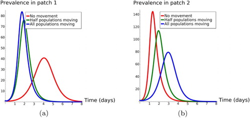
From our simulations in Figure 1, we observe that:

Figure 1. Dynamics of $I_1$ and $I_2$ when we vary $p_{11},p_{12},p_{21}$, $p_{22}$ and have no movement ($p_{11}=p_{22}=1$, $p_{12}=p_{21}=0$), half populations moving ($p_{11}=p_{22}=p_{12}=p_{21}=0.5$), and all populations moving ($p_{11}=p_{22}=0$, $p_{12}=p_{21}=1$). The figure on the left panel shows that the prevalence in patch 1 reaches its highest when in extreme mobility case (blue line) and is lowest when there is no mobility between patches (red line). The figure on the right panel show the opposite of this scenario in patch 2 (high risk). (a) The plot of Infected individuals ($I_1$) in patch 1 and (b) The plot of Infected individuals ($I_2$) in patch 2.

1. For the case of no movement between patches (no mobility), that is, $p_{11}=p_{22}=1$ and $p_{12}=p_{21}=0$, the system behaves as two separated patches where we have the disease prevalence to be at its highest in patch 2.

2. For the symmetric case in which $p_{11}=p_{12}=p_{21}=p_{22}=0.5$, the system has the same level of disease prevalence in both patches.

3. The case where everyone move from their patch to the other patch (high mobility), that is $p_{11}=p_{22}=1$ and $p_{12}=p_{21}=0$, the system has the highest disease prevalence in patch 1.

Our numerical results is similar to [10] where direct transmission pathway is considered as a form of disease spread. Our results show that considering indirect transmission pathway is of great importance and disease spread may be difficult to control (the case of cholera) if otherwise, as in Figure 1.

5. Conclusion

In this paper, we proposed and studied an epidemic model in which infection is transmitted when viruses are shed and acquired through host (population)-source (environment)-host (population) in heterogeneous environments. For the three models developed, we calculated the reproduction number, estimated the initial exponential growth rate and obtained the reproduction number in terms of parameters that can be estimated. The final size relation was also analysed to find the number of disease cases and disease deaths in terms of the model parameters.

We examined an SIVR model with residence times and develop a 2-patch model where infection risk is as a result of the residence time and other environmental factors. With this approach, we studied the disease prevalence in heterogeneous environment through indirect transmission pathways without needing to measure contact rates and our analysis was also buttressed by numerical results.

Our primary result shows that the number of populations being infected through indirect transmission medium which had been omitted in some other previous works is worth taking into account. The result of our numerical simulation is similar to one of the results in [10] in which only direct transmission pathway was considered. We were able to show how worst the prevalence of a disease could be when the disease transmission is indirect.

We considered indirect transmission of viruses in heterogeneous mixing population, but considering direct and indirect pathways (the case of Ebola), may give a different/better insight into the disease prevalence and how accurate treatment will be apportioned.

Despite these limitations, our models can be used to compare disease spread between two populations with different contact rates, such as cities against villages, rich against poor populations and so on. The derivation of the age of infection model could be extended to include direct transmission pathways. It is also possible to extend the model with the residence times to incorporate treatment strategies which may reduce the contact rates and then lower the reproduction number. In addition, it may be more realistic to extend the model to incorporate multiple class of hosts and sources in order to compare the disease spread among different populations and with different viruses.

Acknowledgments

This work was first communicated by Professor Fred Brauer. I sincerely appreciate Fred for weekly discussions, contributions and supports from the beginning and throughout the period of compiling the work. Special thanks to two anonymous reviewers for their valuable comments which have improve the paper significantly.

Disclosure statement

No potential conflict of interest was reported by the author.

Additional information

Funding

This work was supported by the Natural Sciences and Engineering Research Council of Canada (NSERC) under Grant RGPIN-2016-03706.

References

- G. Brankston, L. Gutterman, Z. Hirji, C. Lemieux, and M. Gardam, Transmission of influenza A in human beings, Lancet Infect Dis. 7 (2007), pp. 257–265. doi: 10.1016/S1473-3099(07)70029-4
- F. Brauer, Epidemic models with heterogeneous mixing and treatment, Bull. Math. Biol. 70 (2008), pp. 1869–1885. doi: 10.1007/s11538-008-9326-1
- F. Brauer, Age-of-infection and the final size relation, Math. Biosci. Eng. 5 (2008), pp. 681–690. doi: 10.3934/mbe.2008.5.681
- F. Brauer, A new epidemic model with indirect transmission, J. Biol. Dyn. 11 (2016), pp. 1–10.
- F. Brauer and C. Castillo-Chavez, Mathematical Models in Population Biology and Epidemiology, Vol. 41, Springer, New York, 2012.
- F. Brauer, Z. Feng, and C. Castillo-Chavez, Discrete epidemic models, Math. Biosci. Eng. 7 (2010), pp. 1–15. doi: 10.3934/mbe.2010.7.1
- F. Brauer, C. Castillo-Chavez, A. Mubayi, and S. Towers, Some models for epidemics of vector-transmitted diseases, Infect. Dis. Model. 1 (2016), pp. 79–87.
- C.B. Bridges, M.J. Kuehnert, and C.B. Hall, Transmission of influenza: Implications for control in health care settings, Clin. Infect. Dis. 42 (2003), pp. 1094–1101.
- C. Castillo-Chavez, D. Bichara, and B.R. Morin, Perspectives on the role of mobility, behavior, and time scales in the spread of diseases, Proc. Natl. Acad. Sci. 113 (2016), pp. 14582–14588. doi: 10.1073/pnas.1604994113
- Y.K. Derdei Bichara, C. Castillo-Chavez, R. Horan, and C. Perrings, SIS and SIR epidemic models under virtual dispersal, Bull. Math. Biol. 77 (2015), pp. 2004–2034. doi: 10.1007/s11538-015-0113-5
- B. Espinoza, V. Moreno, D. Bichara, and C. Castillo-Chavez, Assessing the efficiency of movement restriction as a control strategy of Ebola, in Mathematical and Statistical Modeling for Emerging and Re-emerging Infectious Diseases, Springer International Publishing, Cham, 2016, pp. 123–145.
- B. Fred, Heterogeneous mixing in epidemic models, Canad. Appl. Math. Q. 20 (2012), pp. 1–14.
- B. Fred and G. Chowell, On epidemic growth rates and the estimation of the basic reproduction number, pp. 1–27. Available at http://chowell.lab.asu.edu/publication_pdfs/notas_cimat.pdf.
- A. Jaichuang and W. Chinviriyasit, Numerical modelling of influenza model with diffusion, Int. J. Appl. Phys. Math. 4 (2014), pp. 15–21. doi: 10.7763/IJAPM.2014.V4.247
- W.O. Kermack and A.G. McKendrick, A contribution to the mathematical theory of epidemics. Part I, Proc. R. Soc. A 115 (1927), pp. 700–721. doi: 10.1098/rspa.1927.0118
- W.O. Kermack and A.G. McKendrick, Contributions to the mathematical theory of epidemics . II. The problem of endemicity, Proc. R. Soc. A 138 (1932), pp. 55–83. doi: 10.1098/rspa.1932.0171
- W.O. Kermack and A.G. McKendrick, Contributions to the mathematical theory of epidemics . III. Further studies of the problem of endemicity, Proc. R. Soc. A 141 (1932), pp. 94–122. doi: 10.1098/rspa.1933.0106
- J.J. Levin and D.F. Shea, On the asymptotic behaviour of the bounded solutions of some integral equations, I, J. Math. Anal. Appl. 37 (1972), pp. 42–82, 288–326, 537–575. doi: 10.1016/0022-247X(72)90258-2
- Z. Liang, Z.-C. Wang, and Y. Zhang, Dynamics of a reaction–diffusion waterborne pathogen model with direct and indirect transmission, J. Comput. Math. Appl. 72 (2016), pp. 202–215. doi: 10.1016/j.camwa.2016.05.013
- S. Mubareka, A.C. Lowen, J. Steel, A.L. Coates, A. Garcia-Sastre, and P. Palese, Transmission of influenza virus via aerosols and fomites in the guinea pig model, J. Infect. Dis. 199 (2009), pp. 858–865. doi: 10.1086/597073
- J.H. Tien and D.J.D. Earn, Multiple transmission pathways and disease dynamics in a waterborne pathogen model, Bull. Math. Biol. 72 (2010), pp. 1506–1533. doi: 10.1007/s11538-010-9507-6
- P. van den Driessche and J. Watmough, Reproduction numbers and sub-threshold endemic equilibria for compartmental models of disease transmission, Math Biosci. 180 (2002), pp. 29–48. doi: 10.1016/S0025-5564(02)00108-6