A mathematical model of malaria transmission in a periodic environment

ABSTRACT

In this paper, we present a mathematical model of malaria transmission dynamics with age structure for the vector population and a periodic biting rate of female anopheles mosquitoes. The human population is divided into two major categories: the most vulnerable called non-immune and the least vulnerable called semi-immune. By applying the theory of uniform persistence and the Floquet theory with comparison principle, we analyse the stability of the disease-free equilibrium and the behaviour of the model when the basic reproduction ratio ${\mathcal{R}}_0$ is greater than one or less than one. At last, numerical simulations are carried out to illustrate our mathematical results.

KEYWORDS:

• Uniform persistence
• basic reproduction ratio
• stability
• periodic solution
• immunity

AMS CLASSIFICATIONS:

• 37N30
• 37N25
• 65L12
• 65U05

1. Introduction

Malaria is a common and life-threatening infectious disease in many tropical and subtropical areas. It is caused by the Plasmodium parasite which is transmitted by female anopheles mosquitoes while they bite humans for a blood meal for the development of their eggs. During the blood meal, the mosquito injects sporozoites into the blood stream. In few minutes, the sporozoites enter the liver cells where each sporozoite develops into a tissue schizont that contains 10,000 to 30,000 merozoites. After 1–2 weeks, the schizont ruptures and releases the merozoites into the blood stream which then invade the red blood cells. The clinical symptoms of malaria are due to the rupture of the red blood cells and release of the parasites waste and cells debris into the blood stream. Note that human malaria is caused by five different species of Plasmodium: Plasmodium falciparum, Plasmodium malariae, Plasmodium ovale, Plasmodium vivax and Plasmodium knowlesi. However, P. falciparum is the most prevalent in Africa and it causes the highest mortality rate induced by the disease [27]. The biology of the five species of Plasmodium is generally similar and consists of two distinct phases: a sexual stage at the mosquito host and an asexual stage at the human host.

The World Health Organization (WHO) estimated that there were 214 million malaria cases in 2015, resulting in about 438,000 deaths [39]. Moreover, in endemic regions, children under 5, pregnant women and non-immune adults are most at risk of malaria mortality [12]. Indeed, there are currently over 100 countries where there is a risk of malaria transmission, and these are visited by more than 125 million international travellers every year. International travellers to countries with ongoing local malaria transmission arriving from countries with no transmission are at high risk of malaria infection and its consequences because they lack immunity. Migrants from countries with malaria transmission living in malaria-free countries and returning to their home countries to visit friends and relatives are similarly at risk because of waning or lack of immunity. Despite extensive efforts to eradicate it, malaria caused by P. falciparum remains a significant problem. A characteristic of falciparum malaria disease that complicates control efforts is clinical immunity: an immune response that develops with exposure to parasites and provides protection against the clinical symptoms of malaria, despite the presence of parasites [32]. This immunity is not complete and one can lose it and become susceptible after interruption of exposure. Those who have acquired immunity can host and tolerate malaria parasites without developing any clinical symptoms. They may become asymptomatic carriers of parasites and may transmit slightly the parasites to mosquitoes [15, 19, 34].

In order to reduce the spread of infectious diseases, mathematical models have been proposed to study their dynamics [5, 25, 40]. Models can provide estimates of underlying parameters of a real-world problem which are difficult or expensive to obtain through experiment or otherwise [28, 29]. They can predict whether the associated disease will spread through the population or die out [3, 8, 18]. It can also estimate the impact of a control measure and provide useful guidelines to public health for further efforts required for disease elimination.

Concerning the mathematical modelling of malaria, significant breakthroughs have been made in the recent years since the first model introduced by Ronald Ross [31]. According to Ross, if the mosquito population can be reduced to below a certain threshold, then malaria can be eradicated. Some years later, Macdonald [22] improved the model of Ross. He showed that reducing the number of mosquitoes has little effect on epidemiology of malaria in areas of intense transmission. Furthermore, Aron and May [1, 2] added various characteristics of malaria to the model of Macdonald, such as an incubation period in the mosquito, superinfection and a period of immunity in humans. An important addition to the malaria models was the inclusion of acquired immunity proposed by Dietz et al. [9].

Other reviews on mathematical modelling in malaria include Ngwa et al. [26] and Chitnis et al. [6]. Indeed, in the Ngwa and Shu model, humans follow an SEIRS-like pattern and mosquitoes follow an SEI pattern, similar to that described by Yang [42], but with only one immune class for humans. Humans move from the susceptible to the exposed class at some probability when they come into contact with an infectious mosquito, and then to the infectious class, as in conventional SEIRS models. However, infectious people can then recover with, or without, a gain in immunity, and either return to the susceptible class or move to the recovered class. Moreover, Chitnis et al. extended the model of Ngwa and Shu by assuming that although individuals in the recovered class are immune, in the sense that they do not suffer from serious illness and do not contract clinical malaria, they still have low levels of Plasmodium in their blood stream and can pass the infection to susceptible mosquitoes.

Recent works have shown that the age structure of vector population and the climate effects are very important factors on the dynamics of malaria transmission [11, 20, 37] because the dynamics of vector population and the biting rate from mosquitoes to humans are greatly influenced by environmental and climatic factors. In addition, based on the susceptibility, the exposedness and the infectivity of human host, Ducrot et al. [10] have developed a deterministic mathematical model for the transmission of malaria with two host types in the human population. The first type called non-immune is supposed to be very vulnerable to malaria because it has never acquired immunity against the disease. The second type called semi-immune is supposed to be non-vulnerable because it has at least once acquired immunity in his life.

This article is an extension of the model studied in [10] in the sense that we consider the life cycle of vector population and the climatic factors on the biting rate of female anopheles mosquitoes [34]. Thus the model is formulated as a non-autonomous system of differential equations. Through rigorous analysis via theories and methods of dynamical systems [16, 33, 43], we derive the epidemic threshold parameter ${\mathcal{R}}_0$, for predicting disease persistence or extinction in periodic environments and we explore the global stability of the equilibrium state and the existence of positive periodic solution under certain conditions.

This paper is organized as follows. In Section 2, we formulate the mathematical model. In Section 3, we show that the dynamical properties of the model are completely determined by the basic reproduction ratio ${\mathcal{R}}_0$. Computational simulations are provided in Section 4 in order to illustrate our mathematical results. Finally, we conclude in Section 5.

2. Mathematical model formulation

In the study of malaria transmission, it has been shown that the susceptibility and the infectivity of the human host depend on certain genetic factors. These two clinical states depend on whether the host has lost his immunity or if he has not yet acquired it. Indeed, acquired immunity is a very important factor in the dynamics of malaria transmission. Several studies have shown that humans who have never acquired immunity during their lifetime have a very high risk of succumbing to malaria compared to those who have already acquired it at least once in their lifetime [15, 21, 23]. This is the main reason why many children under 5 old years die of malaria in endemic areas. In fact, newborns (from an immunized mother) are protected because of the passive transfer of maternal antibodies through the placenta in the first 3–6 months of life. After these first few months, they are vulnerable to clinical episodes of malaria until they have built their own immunity. Thus, to better understand the dynamics of malaria transmission, it is important to divide human hosts according to their immune status. This will help to develop better strategies against the disease.

Hence, using this assumption, we divide the human population into two major types: the non-immune, namely those who have not acquired immunity (the most vulnerable), and the semi-immune, those who have already acquired their immunity at least once in their life (least vulnerable).

The non-immune population is divided into three epidemiological categories representing the state variables: the susceptible class $S_e$, the exposed class $E_e$ and the infectious class $I_e$. Similarly, the semi-immune population is divided into four epidemiological categories representing the state variables: the susceptible class $S_a$, the exposed class $E_a$, the infectious class $I_a$ and the immune class $R_a$. Humans in the class $R_a$ have some immunity to the disease and do not get clinically ill, but they still harbour low levels of parasite in their blood stream and can pass the infection to the susceptible mosquitoes [6].

Mosquito population is also divided into two major stages: the mature stage (those which can fly) and the aquatic stage (eggs, larvae and pupae). The mature stage is divided into three compartments: the susceptible class $S_v$, the exposed class $E_v$ and the infectious class $I_v$. The immature stage represented by the compartment L is constituted by eggs, larvae and pupae.

At any time t, the total size of humans, $N_h\left(t\right)$, and mature mosquitoes, $N_v\left(t\right)$, is respectively denoted by the following equations: $\begin{array}{rl}{N}_h\left(t\right)& =\left(S_e\left(t\right)+S_a\left(t\right)\right)+\left(E_e\left(t\right)+E_a\left(t\right)\right)+\left(I_e\left(t\right)+I_a\left(t\right)\right)+R_a\left(t\right),\\ N_v\left(t\right)& =S_v\left(t\right)+E_v\left(t\right)+I_v\left(t\right).\end{array}$ Furthermore, we assume throughout this paper that:

(A1)	all vector population measures refer to densities of female anopheles mosquitoes,
(A2)	the mosquitoes bite only humans, with periodic biting rate $\beta \left(t\right)$,
(A3)	there is no direct transmission (blood transfusion or from mother to baby) of malaria,
(A4)	all the new recruits are susceptible. There are no immigrations of infectious humans.

Note that in absence of disease, the vector population dynamics is described by the following diagram .

Hence, according to Figure 1 we obtain the following system: $\begin{array}{rl}{\dot{N}}_v\left(t\right)& =r_{v}L\left(t\right)-d_v{N}_v\left(t\right),\\ \dot{L}\left(t\right)& =b{N}_v\left(t\right)-(d_l+r_v)L\left(t\right).\end{array}$ Moreover, female mosquitoes lay their eggs on the surface of water or near rivers. However, if there are too many eggs in the oviposition habitat or very few nutrients and water resources, then females choose another site or lay less eggs. In addition, to complete their development, larvae and pupae need water or nutrients [24]. Hence, using the logistic growth [41], the per capita oviposition rate is given by $b\left(1-\frac{L\left(t\right)}{K}\right)N_v\left(t\right).$ Finally, we get the following system: (1) $\begin{array}{rl}{\dot{N}}_v\left(t\right)& =r_{v}L\left(t\right)-d_v{N}_v\left(t\right),\\ \dot{L}\left(t\right)& =b\left(1-\frac{L\left(t\right)}{K}\right)N_v\left(t\right)-(d_l+r_v)L\left(t\right),\end{array}$(1) where the biological meaning of parameters b, $r_v$, $d_v$, $d_l$ and K is given in Table 1.

Figure 1. Transfer diagram: the solid arrows represent the transition from one class to another and the blue dashed arrow represents the eggs laying of female mosquitoes.

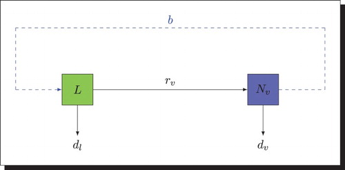
Table 1. Values for constant parameters of the model.

Symbols	Biological descriptions	Values	Sources	Dimensions
Λ	constant recruitment rate for humans	5000	estimated	/month
$d_h$	human death rate	$0.00167$	estimated	/month
${\alpha }_e$	transfer rate of humans from $I_e$ to $R_a$	0.03	[10]	/month
${\alpha }_a$	transfer rate of humans from $E_a$ to $R_a$	0.3	[10]	/month
${\gamma }_e$	disease-induced death rate for non-immune	0.00054	estimated	/month
${\gamma }_a$	disease-induced death rate for semi-immune	0.00027	estimated	/month
${\nu }_e$	transfer rate of humans from $E_e$ to $I_e$	3	[7]	/month
${\nu }_a$	transfer rate of humans from $E_a$ to $I_a$	2.7	[7]	/month
${\beta }_a$	per capita rate of loss of immunity for humans	0.081	[10]	/month
$c_{ev}$	probability of transmission of infection from $I_e$ to $S_v$	0.45	[10]	dimensionless
$c_{av}$	probability of transmission of infection from $I_a$ to $S_v$	0.35	[10]	dimensionless
${\overline{c}}_{av}$	probability of transmission of infection from $R_h$ to $S_v$	0.002	[10]	dimensionless
p	probability of recruitment for humans	0.4	estimated	/month
$r_v$	transfer rate from L to adult	–	estimated	/month
$d_v$	death rate for adult vectors	–	estimated	/month
$c_{ve}$	probability of transmission of infection from $I_v$ to $S_e$	0.07	[10]	dimensionless
$c_{va}$	probability of transmission of infection from $I_v$ to $S_a$	0.022	[10]	dimensionless
${\nu }_v$	transfer rate of mosquitoes from $E_v$ to $I_v$	2.49	[10]	/month
$\beta \left(t\right)$	biting rate of mosquitoes	–	estimated	/month
K	breeder site occupied by immature mosquitoes	150,000	estimated	dimensionless
b	eggs laying rate	–	estimated	/month
$d_l$	death rate of immature mosquitoes	–	estimated	/month

2.1. Interaction between humans and mosquitoes

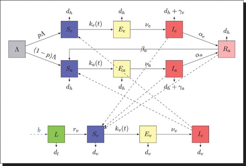
When an infectious mosquito bites a susceptible non-immune, the parasite enters the body of the non-immune with probability $c_{ve}$ and he moves to the exposed class $E_e$. Some time after, he moves from class $E_e$ to the infectious class $I_e$ with constant rate ${\nu }_e$. The infectious non-immune moves to the immune class $R_a$ at rate ${\alpha }_e$ after acquisition of his immunity. The non-immune disappears from the population through natural death rate $d_h$ and malaria death rate ${\gamma }_e$. In the same way, when an infectious mosquito bites a susceptible semi-immune, the parasite enters the body of the semi-immune with probability $c_{va}$ and he moves to the exposed class $E_a$. Some time after, he moves from class $E_a$ to the infectious class $I_a$ with constant rate ${\nu }_a$. By immunology memory, immunity of infectious semi-immune might be rapidly restored at rate ${\alpha }_a$ when they begin to be re-exposed to infection. Immune individuals in class $R_a$ can lose their immunity at rate ${\beta }_a$ and go back to susceptible class $S_a$. The infectious semi-immune leaves the population through natural death rate $d_h$ and malaria death rate ${\gamma }_a$ (${\gamma }_a\le {\gamma }_e$). At any time, the non-immune population receives a new recruitment, $p\mathrm{\Lambda }$, and the semi-immune population receives a new recruitment, $(1-p)\mathrm{\Lambda }$, with $p\in [0,1]$.

Similarly, when a susceptible mosquito bites an infectious non-immune (resp. semi-immune, immune), it enters the class $E_v$ with a probability $c_{ev}$ (resp. $c_{av},{\tilde{c}}_{av}$). Some time after, it moves from class $E_v$ to the infectious class $I_v$ with rate ${\nu }_v$ where it stays for life. Mature mosquitoes disappear from the population through natural mortality $d_v$.

Using the standard incidence as in the model of Ngwa and Shu [26], we define respectively the infection incidence from mosquitoes to non-immune, $k_e\left(t\right)$, from mosquitoes to semi-immune, $k_a\left(t\right)$, and from humans to mosquitoes, $k_v\left(t\right)$. $\begin{array}{rl}{k}_e\left(t\right)& =c_{ve}\beta \left(t\right)\frac{I_v\left(t\right)}{N_h\left(t\right)},\\ k_a\left(t\right)& =c_{va}\beta \left(t\right)\frac{I_v\left(t\right)}{N_h\left(t\right)},\\ k_v\left(t\right)& =c_{av}\beta \left(t\right)\frac{I_a\left(t\right)}{N_h\left(t\right)}+c_{ev}\beta \left(t\right)\frac{I_e\left(t\right)}{N_h\left(t\right)}+{\tilde{c}}_{av}\beta \left(t\right)\frac{R_a\left(t\right)}{N_h\left(t\right)}.\end{array}$ According to the above assumptions, we get the following schematic diagram (Figure 2) .

Figure 2. Transfer diagram: the black dashed arrows indicate the direction of the infection, the solid arrows represent the transition from one class to another and the blue dashed arrow represents the eggs laying of female mosquitoes.

2.2. Mathematical model

Using the above assumptions and by making a balance of the movements in each class, we obtain the following system: (2) $\begin{array}{rl}\dot{S_e}\left(t\right)& =p\mathrm{\Lambda }-\left(k_e\right(t)+d_h)S_e\left(t\right),\\ \dot{E_e}\left(t\right)& =k_e\left(t\right)S_e\left(t\right)-({\nu }_e+d_h)E_e\left(t\right),\\ \dot{I_e}\left(t\right)& ={\nu }_e{E}_e\left(t\right)-{\alpha }_e{I}_e\left(t\right)-(d_h+{\gamma }_e)I_e\left(t\right),\\ \dot{S_a}\left(t\right)& =(1-p)\mathrm{\Lambda }+{\beta }_a{R}_a\left(t\right)-\left(k_a\right(t)+d_h)S_a\left(t\right),\\ \dot{E_a}\left(t\right)& =k_a\left(t\right)S_a\left(t\right)-(d_h+{\nu }_a)E_a\left(t\right),\\ \dot{I_a}\left(t\right)& ={\nu }_a{E}_a\left(t\right)-d_h{I}_a\left(t\right)-({\alpha }_a+{\gamma }_a)I_a\left(t\right),\\ \dot{R_a}\left(t\right)& ={\alpha }_e{I}_e\left(t\right)+{\alpha }_a{I}_a\left(t\right)-(d_h+{\beta }_a)R_a\left(t\right),\\ \dot{L}\left(t\right)& =b\left(1-\frac{L\left(t\right)}{K}\right)\left(S_v\left(t\right)+E_v\left(t\right)+I_v\left(t\right)\right)-(d_l+r_v)L\left(t\right),\\ {\dot{S}}_v\left(t\right)& =r_{v}L\left(t\right)-(d_v+k_v(t\left)\right)S_v\left(t\right),\\ {\dot{E}}_v\left(t\right)& =k_v\left(t\right)S_v\left(t\right)-(d_v+{\nu }_v)E_v\left(t\right),\\ {\dot{I}}_v\left(t\right)& ={\nu }_v{E}_v\left(t\right)-d_v{I}_v\left(t\right),\end{array}$(2) with initial conditions: $\begin{array}{rl}& S_e\left(0\right)>0,E_e\left(0\right)>0,I_e\left(0\right)>0,\\ & S_a\left(0\right)>0,E_a\left(0\right)>0,I_a\left(0\right)>0,R_a\left(0\right)>0,\\ & L\left(0\right)>0,S_v\left(0\right)>0,E_v\left(0\right)>0,I_v\left(0\right)>0.\end{array}$ The growth of the whole human population and mature vector is respectively described by the following equations: (3) ${\dot{N}}_h\left(t\right)=\mathrm{\Lambda }-d_h{N}_h\left(t\right)-{\gamma }_e{I}_e\left(t\right)-{\gamma }_a{I}_a\left(t\right),$(3) (4) ${\dot{N}}_v\left(t\right)=r_{v}L\left(t\right)-d_v{N}_v\left(t\right).$(4) The evolution of the immature mosquitoes is described by the following equation: (5) $\dot{L}\left(t\right)=b\left(1-\frac{L\left(t\right)}{K}\right)N_v\left(t\right)-(d_l+r_v)L\left(t\right).$(5) Hence, the system (2(2) $\begin{array}{rl}\dot{S_e}\left(t\right)& =p\mathrm{\Lambda }-\left(k_e\right(t)+d_h)S_e\left(t\right),\\ \dot{E_e}\left(t\right)& =k_e\left(t\right)S_e\left(t\right)-({\nu }_e+d_h)E_e\left(t\right),\\ \dot{I_e}\left(t\right)& ={\nu }_e{E}_e\left(t\right)-{\alpha }_e{I}_e\left(t\right)-(d_h+{\gamma }_e)I_e\left(t\right),\\ \dot{S_a}\left(t\right)& =(1-p)\mathrm{\Lambda }+{\beta }_a{R}_a\left(t\right)-\left(k_a\right(t)+d_h)S_a\left(t\right),\\ \dot{E_a}\left(t\right)& =k_a\left(t\right)S_a\left(t\right)-(d_h+{\nu }_a)E_a\left(t\right),\\ \dot{I_a}\left(t\right)& ={\nu }_a{E}_a\left(t\right)-d_h{I}_a\left(t\right)-({\alpha }_a+{\gamma }_a)I_a\left(t\right),\\ \dot{R_a}\left(t\right)& ={\alpha }_e{I}_e\left(t\right)+{\alpha }_a{I}_a\left(t\right)-(d_h+{\beta }_a)R_a\left(t\right),\\ \dot{L}\left(t\right)& =b\left(1-\frac{L\left(t\right)}{K}\right)\left(S_v\left(t\right)+E_v\left(t\right)+I_v\left(t\right)\right)-(d_l+r_v)L\left(t\right),\\ {\dot{S}}_v\left(t\right)& =r_{v}L\left(t\right)-(d_v+k_v(t\left)\right)S_v\left(t\right),\\ {\dot{E}}_v\left(t\right)& =k_v\left(t\right)S_v\left(t\right)-(d_v+{\nu }_v)E_v\left(t\right),\\ {\dot{I}}_v\left(t\right)& ={\nu }_v{E}_v\left(t\right)-d_v{I}_v\left(t\right),\end{array}$(2) ) can be written as follows: $\begin{array}{rl}& \dot{Z}\left(t\right)=g(t,Z(t\left)\right),\\ & Z\left(0\right)>0,\end{array}$ where $Z\left(t\right)={\left(S_e\left(t\right),E_e\left(t\right),I_e\left(t\right),S_a\left(t\right),E_a\left(t\right),I_a\left(t\right),R_a\left(t\right),L\left(t\right),S_v\left(t\right),E_v\left(t\right),I_v\left(t\right)\right)}^{\mathrm{T}}$ and $g:{\mathbb{R}}_{+}\times {\mathbb{R}}^{11}⟶{\mathbb{R}}^{11}$ defined by $g\left(t,Z\left(t\right)\right)=\left(\begin{array}{c}p\mathrm{\Lambda }-k_e\left(t\right)S_e\left(t\right)-d_h{S}_e\left(t\right)\\ k_e\left(t\right)S_e\left(t\right)-{\nu }_e{E}_e\left(t\right)-d_h{E}_e\left(t\right)\\ {\nu }_e{E}_e\left(t\right)-{\alpha }_e{I}_e\left(t\right)-d_h{I}_e\left(t\right)-{\gamma }_e{I}_e\left(t\right)\\ (1-p)\mathrm{\Lambda }+{\beta }_a{R}_a\left(t\right)-k_a\left(t\right)S_a\left(t\right)-d_h{S}_a\left(t\right)\\ k_a\left(t\right)S_a\left(t\right)-d_h{E}_a\left(t\right)-{\nu }_a{E}_a\left(t\right)\\ {\nu }_a{E}_a\left(t\right)-d_h{I}_a\left(t\right)-{\alpha }_a{I}_a\left(t\right)-{\gamma }_a{I}_a\left(t\right)\\ {\alpha }_e{I}_e\left(t\right)-d_h{R}_a\left(t\right)+{\alpha }_a{I}_a\left(t\right)-{\beta }_a{R}_a\left(t\right)\\ b\left(1-\frac{L\left(t\right)}{K}\right)N_v\left(t\right)-(d_l+r_v)L\left(t\right)\\ r_{v}L\left(t\right)-d_v{S}_v\left(t\right)-k_v\left(t\right)S_v\left(t\right)\\ k_v\left(t\right)S_v\left(t\right)-d_v{E}_v\left(t\right)-{\nu }_v{E}_v\left(t\right)\\ {\nu }_v{E}_v\left(t\right)-d_v{I}_v\left(t\right)\end{array}\right).$ We assume that

1. the biting rate $\beta \left(t\right)$ is a continuous ω-periodic positive function with $\omega =12$ months,

2. all the parameters of the model are positive except the disease-induced death rates, ${\gamma }_e$ and ${\gamma }_a$, which are assumed to be non-negative.

3. Mathematical analysis

3.1. Positivity and boundedness of solutions

Lemma 3.1

For any positive initial condition, $\phi =\left(S_e\right(0),E_e(0),I_e(0),S_a(0),E_a(0),I_a(0),R_a(0),L(0),S_v(0),E_v(0),I_v(0\left)\right),$ the system (2(2) $\begin{array}{rl}\dot{S_e}\left(t\right)& =p\mathrm{\Lambda }-\left(k_e\right(t)+d_h)S_e\left(t\right),\\ \dot{E_e}\left(t\right)& =k_e\left(t\right)S_e\left(t\right)-({\nu }_e+d_h)E_e\left(t\right),\\ \dot{I_e}\left(t\right)& ={\nu }_e{E}_e\left(t\right)-{\alpha }_e{I}_e\left(t\right)-(d_h+{\gamma }_e)I_e\left(t\right),\\ \dot{S_a}\left(t\right)& =(1-p)\mathrm{\Lambda }+{\beta }_a{R}_a\left(t\right)-\left(k_a\right(t)+d_h)S_a\left(t\right),\\ \dot{E_a}\left(t\right)& =k_a\left(t\right)S_a\left(t\right)-(d_h+{\nu }_a)E_a\left(t\right),\\ \dot{I_a}\left(t\right)& ={\nu }_a{E}_a\left(t\right)-d_h{I}_a\left(t\right)-({\alpha }_a+{\gamma }_a)I_a\left(t\right),\\ \dot{R_a}\left(t\right)& ={\alpha }_e{I}_e\left(t\right)+{\alpha }_a{I}_a\left(t\right)-(d_h+{\beta }_a)R_a\left(t\right),\\ \dot{L}\left(t\right)& =b\left(1-\frac{L\left(t\right)}{K}\right)\left(S_v\left(t\right)+E_v\left(t\right)+I_v\left(t\right)\right)-(d_l+r_v)L\left(t\right),\\ {\dot{S}}_v\left(t\right)& =r_{v}L\left(t\right)-(d_v+k_v(t\left)\right)S_v\left(t\right),\\ {\dot{E}}_v\left(t\right)& =k_v\left(t\right)S_v\left(t\right)-(d_v+{\nu }_v)E_v\left(t\right),\\ {\dot{I}}_v\left(t\right)& ={\nu }_v{E}_v\left(t\right)-d_v{I}_v\left(t\right),\end{array}$(2) ) has a unique positive solution $u(t,\phi )$ for all $t\ge 0$.

Proof.

For any positive initial condition φ, the function $g(t,\phi )$ is continuous in $(t,\phi )$ and Lipschitzian in φ. So, thanks to Theorems 2.2.1 and 2.2.3 of Hale and Verduyn Lunel [13], the system (2(2) $\begin{array}{rl}\dot{S_e}\left(t\right)& =p\mathrm{\Lambda }-\left(k_e\right(t)+d_h)S_e\left(t\right),\\ \dot{E_e}\left(t\right)& =k_e\left(t\right)S_e\left(t\right)-({\nu }_e+d_h)E_e\left(t\right),\\ \dot{I_e}\left(t\right)& ={\nu }_e{E}_e\left(t\right)-{\alpha }_e{I}_e\left(t\right)-(d_h+{\gamma }_e)I_e\left(t\right),\\ \dot{S_a}\left(t\right)& =(1-p)\mathrm{\Lambda }+{\beta }_a{R}_a\left(t\right)-\left(k_a\right(t)+d_h)S_a\left(t\right),\\ \dot{E_a}\left(t\right)& =k_a\left(t\right)S_a\left(t\right)-(d_h+{\nu }_a)E_a\left(t\right),\\ \dot{I_a}\left(t\right)& ={\nu }_a{E}_a\left(t\right)-d_h{I}_a\left(t\right)-({\alpha }_a+{\gamma }_a)I_a\left(t\right),\\ \dot{R_a}\left(t\right)& ={\alpha }_e{I}_e\left(t\right)+{\alpha }_a{I}_a\left(t\right)-(d_h+{\beta }_a)R_a\left(t\right),\\ \dot{L}\left(t\right)& =b\left(1-\frac{L\left(t\right)}{K}\right)\left(S_v\left(t\right)+E_v\left(t\right)+I_v\left(t\right)\right)-(d_l+r_v)L\left(t\right),\\ {\dot{S}}_v\left(t\right)& =r_{v}L\left(t\right)-(d_v+k_v(t\left)\right)S_v\left(t\right),\\ {\dot{E}}_v\left(t\right)& =k_v\left(t\right)S_v\left(t\right)-(d_v+{\nu }_v)E_v\left(t\right),\\ {\dot{I}}_v\left(t\right)& ={\nu }_v{E}_v\left(t\right)-d_v{I}_v\left(t\right),\end{array}$(2) ) has a unique solution $u(t,\phi )$ on its maximal interval $[0,t_{max})$ of existence.

Moreover, for all $t\ge 0$, let $e\left(t\right)=min\left\{S_e\left(t\right),E_e\left(t\right),I_e\left(t\right),S_a\left(t\right),E_a\left(t\right),I_a\left(t\right),R_a\left(t\right),L\left(t\right),S_v\left(t\right),E_v\left(t\right),I_v\left(t\right)\right\}.$ Let us suppose that there exists $t_1>0$ such that $e\left(t_1\right)\notin {\mathbb{R}}_{+}^{\ast }$ and $e\left(t\right)>0$ for all $t\in [0,t_1)$.

If $e\left(t\right)=S_e\left(t\right)$, then $S_e\left(t\right)>0$ and $k_e\left(t\right)>0$. Thus, from the first equation of system (2(2) $\begin{array}{rl}\dot{S_e}\left(t\right)& =p\mathrm{\Lambda }-\left(k_e\right(t)+d_h)S_e\left(t\right),\\ \dot{E_e}\left(t\right)& =k_e\left(t\right)S_e\left(t\right)-({\nu }_e+d_h)E_e\left(t\right),\\ \dot{I_e}\left(t\right)& ={\nu }_e{E}_e\left(t\right)-{\alpha }_e{I}_e\left(t\right)-(d_h+{\gamma }_e)I_e\left(t\right),\\ \dot{S_a}\left(t\right)& =(1-p)\mathrm{\Lambda }+{\beta }_a{R}_a\left(t\right)-\left(k_a\right(t)+d_h)S_a\left(t\right),\\ \dot{E_a}\left(t\right)& =k_a\left(t\right)S_a\left(t\right)-(d_h+{\nu }_a)E_a\left(t\right),\\ \dot{I_a}\left(t\right)& ={\nu }_a{E}_a\left(t\right)-d_h{I}_a\left(t\right)-({\alpha }_a+{\gamma }_a)I_a\left(t\right),\\ \dot{R_a}\left(t\right)& ={\alpha }_e{I}_e\left(t\right)+{\alpha }_a{I}_a\left(t\right)-(d_h+{\beta }_a)R_a\left(t\right),\\ \dot{L}\left(t\right)& =b\left(1-\frac{L\left(t\right)}{K}\right)\left(S_v\left(t\right)+E_v\left(t\right)+I_v\left(t\right)\right)-(d_l+r_v)L\left(t\right),\\ {\dot{S}}_v\left(t\right)& =r_{v}L\left(t\right)-(d_v+k_v(t\left)\right)S_v\left(t\right),\\ {\dot{E}}_v\left(t\right)& =k_v\left(t\right)S_v\left(t\right)-(d_v+{\nu }_v)E_v\left(t\right),\\ {\dot{I}}_v\left(t\right)& ={\nu }_v{E}_v\left(t\right)-d_v{I}_v\left(t\right),\end{array}$(2) ), we have ${\dot{S}}_e\left(t\right)>-\left(k_e\right(t)+d_h)S_e\left(t\right).$ It then follows that $S_e\left(t_1\right)>S_e\left(0\right)\exp \left[-{\int }_0^{t_1}\left(k_e\right(t)+d_h)\mathrm{d}t\right]>0,$ which leads to a contradiction.

If $e\left(t\right)=E_e\left(t\right)$, then $S_e\left(t\right)>0$ and $k_e\left(t\right)>0$. Thus, from the second equation of system (2(2) $\begin{array}{rl}\dot{S_e}\left(t\right)& =p\mathrm{\Lambda }-\left(k_e\right(t)+d_h)S_e\left(t\right),\\ \dot{E_e}\left(t\right)& =k_e\left(t\right)S_e\left(t\right)-({\nu }_e+d_h)E_e\left(t\right),\\ \dot{I_e}\left(t\right)& ={\nu }_e{E}_e\left(t\right)-{\alpha }_e{I}_e\left(t\right)-(d_h+{\gamma }_e)I_e\left(t\right),\\ \dot{S_a}\left(t\right)& =(1-p)\mathrm{\Lambda }+{\beta }_a{R}_a\left(t\right)-\left(k_a\right(t)+d_h)S_a\left(t\right),\\ \dot{E_a}\left(t\right)& =k_a\left(t\right)S_a\left(t\right)-(d_h+{\nu }_a)E_a\left(t\right),\\ \dot{I_a}\left(t\right)& ={\nu }_a{E}_a\left(t\right)-d_h{I}_a\left(t\right)-({\alpha }_a+{\gamma }_a)I_a\left(t\right),\\ \dot{R_a}\left(t\right)& ={\alpha }_e{I}_e\left(t\right)+{\alpha }_a{I}_a\left(t\right)-(d_h+{\beta }_a)R_a\left(t\right),\\ \dot{L}\left(t\right)& =b\left(1-\frac{L\left(t\right)}{K}\right)\left(S_v\left(t\right)+E_v\left(t\right)+I_v\left(t\right)\right)-(d_l+r_v)L\left(t\right),\\ {\dot{S}}_v\left(t\right)& =r_{v}L\left(t\right)-(d_v+k_v(t\left)\right)S_v\left(t\right),\\ {\dot{E}}_v\left(t\right)& =k_v\left(t\right)S_v\left(t\right)-(d_v+{\nu }_v)E_v\left(t\right),\\ {\dot{I}}_v\left(t\right)& ={\nu }_v{E}_v\left(t\right)-d_v{I}_v\left(t\right),\end{array}$(2) ), we have ${\dot{E}}_e\left(t\right)>-(d_h+{\nu }_e)E_e\left(t\right).$ It then follows that $E_e\left(t_1\right)>E_e\left(0\right)\exp \left[-(d_h+{\nu }_e)t_1\right]>0,$ which leads to a contradiction.

If $e\left(t\right)=I_e\left(t\right)$, then $E_e\left(t\right)>0$. Thus, from the third equation of system (2(2) $\begin{array}{rl}\dot{S_e}\left(t\right)& =p\mathrm{\Lambda }-\left(k_e\right(t)+d_h)S_e\left(t\right),\\ \dot{E_e}\left(t\right)& =k_e\left(t\right)S_e\left(t\right)-({\nu }_e+d_h)E_e\left(t\right),\\ \dot{I_e}\left(t\right)& ={\nu }_e{E}_e\left(t\right)-{\alpha }_e{I}_e\left(t\right)-(d_h+{\gamma }_e)I_e\left(t\right),\\ \dot{S_a}\left(t\right)& =(1-p)\mathrm{\Lambda }+{\beta }_a{R}_a\left(t\right)-\left(k_a\right(t)+d_h)S_a\left(t\right),\\ \dot{E_a}\left(t\right)& =k_a\left(t\right)S_a\left(t\right)-(d_h+{\nu }_a)E_a\left(t\right),\\ \dot{I_a}\left(t\right)& ={\nu }_a{E}_a\left(t\right)-d_h{I}_a\left(t\right)-({\alpha }_a+{\gamma }_a)I_a\left(t\right),\\ \dot{R_a}\left(t\right)& ={\alpha }_e{I}_e\left(t\right)+{\alpha }_a{I}_a\left(t\right)-(d_h+{\beta }_a)R_a\left(t\right),\\ \dot{L}\left(t\right)& =b\left(1-\frac{L\left(t\right)}{K}\right)\left(S_v\left(t\right)+E_v\left(t\right)+I_v\left(t\right)\right)-(d_l+r_v)L\left(t\right),\\ {\dot{S}}_v\left(t\right)& =r_{v}L\left(t\right)-(d_v+k_v(t\left)\right)S_v\left(t\right),\\ {\dot{E}}_v\left(t\right)& =k_v\left(t\right)S_v\left(t\right)-(d_v+{\nu }_v)E_v\left(t\right),\\ {\dot{I}}_v\left(t\right)& ={\nu }_v{E}_v\left(t\right)-d_v{I}_v\left(t\right),\end{array}$(2) ), we have ${\dot{I}}_e\left(t\right)>-({\alpha }_e+d_h+{\gamma }_e)I_e\left(t\right).$ It then follows that $I_e\left(t_1\right)>I_e\left(0\right)\exp \left[-({\alpha }_e+d_h+{\gamma }_e)t_1\right]>0,$ which leads to a contradiction.

Similar contradictions can be obtained if $e\left(t\right)=S_a\left(t\right)$, $e\left(t\right)=E_a\left(t\right)$, $e\left(t\right)=I_a\left(t\right)$, $e\left(t\right)=R_a\left(t\right)$, $e\left(t\right)=L\left(t\right)$, $e\left(t\right)=S_v\left(t\right)$, $e\left(t\right)=E_v\left(t\right)$ and $e\left(t\right)=I_v\left(t\right)$. Hence, the solution $u(t,\phi )$ is positive.

Thus the system (2(2) $\begin{array}{rl}\dot{S_e}\left(t\right)& =p\mathrm{\Lambda }-\left(k_e\right(t)+d_h)S_e\left(t\right),\\ \dot{E_e}\left(t\right)& =k_e\left(t\right)S_e\left(t\right)-({\nu }_e+d_h)E_e\left(t\right),\\ \dot{I_e}\left(t\right)& ={\nu }_e{E}_e\left(t\right)-{\alpha }_e{I}_e\left(t\right)-(d_h+{\gamma }_e)I_e\left(t\right),\\ \dot{S_a}\left(t\right)& =(1-p)\mathrm{\Lambda }+{\beta }_a{R}_a\left(t\right)-\left(k_a\right(t)+d_h)S_a\left(t\right),\\ \dot{E_a}\left(t\right)& =k_a\left(t\right)S_a\left(t\right)-(d_h+{\nu }_a)E_a\left(t\right),\\ \dot{I_a}\left(t\right)& ={\nu }_a{E}_a\left(t\right)-d_h{I}_a\left(t\right)-({\alpha }_a+{\gamma }_a)I_a\left(t\right),\\ \dot{R_a}\left(t\right)& ={\alpha }_e{I}_e\left(t\right)+{\alpha }_a{I}_a\left(t\right)-(d_h+{\beta }_a)R_a\left(t\right),\\ \dot{L}\left(t\right)& =b\left(1-\frac{L\left(t\right)}{K}\right)\left(S_v\left(t\right)+E_v\left(t\right)+I_v\left(t\right)\right)-(d_l+r_v)L\left(t\right),\\ {\dot{S}}_v\left(t\right)& =r_{v}L\left(t\right)-(d_v+k_v(t\left)\right)S_v\left(t\right),\\ {\dot{E}}_v\left(t\right)& =k_v\left(t\right)S_v\left(t\right)-(d_v+{\nu }_v)E_v\left(t\right),\\ {\dot{I}}_v\left(t\right)& ={\nu }_v{E}_v\left(t\right)-d_v{I}_v\left(t\right),\end{array}$(2) ) is mathematically well-defined over the whole ${\mathbb{R}}_{+}^{11}$. Nevertheless, the region of biological interest is Γ defined by $\mathrm{\Gamma }=\left\{\left(S_e,E_e,I_e,S_a,E_a,I_a,R_a,L,S_v,E_v,I_v\right)\in {\mathbb{R}}_{+}^{11}\left|\begin{array}{c}{N}_h\le \frac{\mathrm{\Lambda }}{d_h}\\ L\le K\\ N_v\le \frac{r_{v}K}{d_v}\end{array}\right.\right\}.$

Lemma 3.2

The compact Γ is a positively invariant set, which attracts all positive orbits in ${\mathbb{R}}_{+}^{11}$. Moreover, all the solutions are bounded.

Proof.

According to Equations (3(3) ${\dot{N}}_h\left(t\right)=\mathrm{\Lambda }-d_h{N}_h\left(t\right)-{\gamma }_e{I}_e\left(t\right)-{\gamma }_a{I}_a\left(t\right),$(3) ), (4(4) ${\dot{N}}_v\left(t\right)=r_{v}L\left(t\right)-d_v{N}_v\left(t\right).$(4) ) and (5(5) $\dot{L}\left(t\right)=b\left(1-\frac{L\left(t\right)}{K}\right)N_v\left(t\right)-(d_l+r_v)L\left(t\right).$(5) ), we have $\begin{array}{rl}{\dot{N}}_h\left(t\right)& =\mathrm{\Lambda }-d_h{N}_h\left(t\right)-{\gamma }_e{I}_e\left(t\right)-{\gamma }_a{I}_a\left(t\right)\le \mathrm{\Lambda }-d_h{N}_h\left(t\right),\\ {\dot{N}}_v\left(t\right)& =r_{v}L\left(t\right)-d_v{N}_v\left(t\right)\le r_{v}K-d_v{N}_v\left(t\right),\\ \dot{L}\left(t\right)& =b\left(1-\frac{L\left(t\right)}{K}\right)N_v\left(t\right)-(d_l+r_v)L\left(t\right)\le \frac{b{r}_{v}K}{d_v}-\frac{b{r}_v}{d_v}L\left(t\right).\end{array}$ Thus if $N_h\left(t\right)>\frac{\mathrm{\Lambda }}{d_h},N_v\left(t\right)>\frac{r_{v}K}{d_v}\text{and}L\left(t\right)>K,$ then ${\dot{N}}_h\left(t\right)<0,{\dot{N}}_v\left(t\right)<0\text{and}\dot{L}\left(t\right)<0,\text{respectively}.$ Moreover, let us consider the following ordinary differential equations: $\begin{array}{rl}{\dot{N}}_h\left(t\right)& =\mathrm{\Lambda }-d_h{N}_h\left(t\right),\\ \dot{L}\left(t\right)& =\frac{b{r}_{v}K}{d_v}-\frac{b{r}_v}{d_v}L\left(t\right),\\ {\dot{N}}_v\left(t\right)& =r_{v}K-d_v{N}_v\left(t\right),\end{array}$ with respective general solutions: $\begin{array}{rl}{N}_h\left(t\right)& =\frac{\mathrm{\Lambda }}{d_h}+\left(N_h\left(0\right)-\frac{\mathrm{\Lambda }}{d_h}\right)\exp (-d_{h}t),\\ N_v\left(t\right)& =\frac{r_{v}K}{d_v}+\left(N_v\left(0\right)-\frac{r_{v}K}{d_v}\right)\exp (-d_{v}t),\\ L\left(t\right)& =K+\left(L\left(0\right)-K\right)\exp \left(-\frac{b{r}_v}{d_v}t\right).\end{array}$ By applying the standard comparison theorem, we have for all $t\ge 0$, $\begin{array}{rl}{N}_h\left(t\right)& \le \frac{\mathrm{\Lambda }}{d_h},\text{if}{N}_h\left(0\right)\le \frac{\mathrm{\Lambda }}{d_h},\\ N_v\left(t\right)& \le \frac{r_{v}K}{d_v},\text{if}{N}_v\left(0\right)\le \frac{r_{v}K}{d_v},\\ L\left(t\right)& \le K,\text{if}L\left(0\right)\le K.\end{array}$ Thus the compact set Γ is positively invariant, and then the solutions are bounded.

3.2. Disease-free equilibria

Let us consider the following threshold parameter: $\kappa =\left(\frac{b}{d_l+r_v}\right)\left(\frac{r_v}{d_v}\right).$ This threshold plays an important role in the dynamics of malaria transmission because it allows to regulate the mosquitoes population dynamics.

Proposition 3.3

The model (2(2) $\begin{array}{rl}\dot{S_e}\left(t\right)& =p\mathrm{\Lambda }-\left(k_e\right(t)+d_h)S_e\left(t\right),\\ \dot{E_e}\left(t\right)& =k_e\left(t\right)S_e\left(t\right)-({\nu }_e+d_h)E_e\left(t\right),\\ \dot{I_e}\left(t\right)& ={\nu }_e{E}_e\left(t\right)-{\alpha }_e{I}_e\left(t\right)-(d_h+{\gamma }_e)I_e\left(t\right),\\ \dot{S_a}\left(t\right)& =(1-p)\mathrm{\Lambda }+{\beta }_a{R}_a\left(t\right)-\left(k_a\right(t)+d_h)S_a\left(t\right),\\ \dot{E_a}\left(t\right)& =k_a\left(t\right)S_a\left(t\right)-(d_h+{\nu }_a)E_a\left(t\right),\\ \dot{I_a}\left(t\right)& ={\nu }_a{E}_a\left(t\right)-d_h{I}_a\left(t\right)-({\alpha }_a+{\gamma }_a)I_a\left(t\right),\\ \dot{R_a}\left(t\right)& ={\alpha }_e{I}_e\left(t\right)+{\alpha }_a{I}_a\left(t\right)-(d_h+{\beta }_a)R_a\left(t\right),\\ \dot{L}\left(t\right)& =b\left(1-\frac{L\left(t\right)}{K}\right)\left(S_v\left(t\right)+E_v\left(t\right)+I_v\left(t\right)\right)-(d_l+r_v)L\left(t\right),\\ {\dot{S}}_v\left(t\right)& =r_{v}L\left(t\right)-(d_v+k_v(t\left)\right)S_v\left(t\right),\\ {\dot{E}}_v\left(t\right)& =k_v\left(t\right)S_v\left(t\right)-(d_v+{\nu }_v)E_v\left(t\right),\\ {\dot{I}}_v\left(t\right)& ={\nu }_v{E}_v\left(t\right)-d_v{I}_v\left(t\right),\end{array}$(2) ) has a:

• trivial disease-free equilibrium $E^{-}=(S_e^{\ast },0,0,S_a^{\ast },0,0,0,0,0,0,0)\text{if}\kappa \le 1,$

• non-trivial disease-free equilibrium $E^{+}=(S_e^{\ast },0,0,S_a^{\ast },0,0,0,L^{\ast },S_v^{\ast },0,0)\text{if}\kappa >1,$ where $S_e^{\ast }=p\frac{\mathrm{\Lambda }}{d_h},S_a^{\ast }=(1-p)\frac{\mathrm{\Lambda }}{d_h},$ and $L^{\ast }=K\left(1-\frac{1}{\kappa }\right),S_v^{\ast }=\frac{r_{v}K}{d_v}\left(1-\frac{1}{\kappa }\right).$

Proof.

Solving the system at the disease-free equilibrium, we get $S_e^{\ast }=p\frac{\mathrm{\Lambda }}{d_h},S_a^{\ast }=(1-p)\frac{\mathrm{\Lambda }}{d_h},S_v^{\ast }=\frac{r_v}{d_v}{L}^{\ast },$ and (6) $b\left(1-\frac{L^{\ast }}{K}\right)S_v^{\ast }-(d_l+r_v)L^{\ast }=0.$(6) Replacing $S_v^{\ast }$ by its expression in (6(6) $b\left(1-\frac{L^{\ast }}{K}\right)S_v^{\ast }-(d_l+r_v)L^{\ast }=0.$(6) ), we have $b\left(1-\frac{L^{\ast }}{K}\right)\frac{r_v}{d_v}{L}^{\ast }-(d_l+r_v)L^{\ast }=0.$ Hence, it yields that $L^{\ast }=0\text{or}{L}^{\ast }=K\left(1-\frac{d_v(d_l+r_v)}{b{r}_v}\right)=K\left(1-\frac{1}{\kappa }\right).$ Thus

• If $\kappa \le 1$, $L^{\ast }=0$, then $S_v^{\ast }=0$. Hence, we obtain $E^{-}$.

• If $\kappa >1$, $L^{\ast }>0$, then $S_v^{\ast }=\left(r_{v}K/d_v\right)(1-1/\kappa )$. Hence, we obtain $E^{+}$.

Remark 3.1

In practice, it is very difficult to find regions completely devoid of anopheles. Hence, we only consider the non-trivial disease-free equilibrium because it is more biologically realistic. So, in the rest of the paper we assume that $\kappa >1$.

3.3. Threshold dynamics

Linearizing the system (2(2) $\begin{array}{rl}\dot{S_e}\left(t\right)& =p\mathrm{\Lambda }-\left(k_e\right(t)+d_h)S_e\left(t\right),\\ \dot{E_e}\left(t\right)& =k_e\left(t\right)S_e\left(t\right)-({\nu }_e+d_h)E_e\left(t\right),\\ \dot{I_e}\left(t\right)& ={\nu }_e{E}_e\left(t\right)-{\alpha }_e{I}_e\left(t\right)-(d_h+{\gamma }_e)I_e\left(t\right),\\ \dot{S_a}\left(t\right)& =(1-p)\mathrm{\Lambda }+{\beta }_a{R}_a\left(t\right)-\left(k_a\right(t)+d_h)S_a\left(t\right),\\ \dot{E_a}\left(t\right)& =k_a\left(t\right)S_a\left(t\right)-(d_h+{\nu }_a)E_a\left(t\right),\\ \dot{I_a}\left(t\right)& ={\nu }_a{E}_a\left(t\right)-d_h{I}_a\left(t\right)-({\alpha }_a+{\gamma }_a)I_a\left(t\right),\\ \dot{R_a}\left(t\right)& ={\alpha }_e{I}_e\left(t\right)+{\alpha }_a{I}_a\left(t\right)-(d_h+{\beta }_a)R_a\left(t\right),\\ \dot{L}\left(t\right)& =b\left(1-\frac{L\left(t\right)}{K}\right)\left(S_v\left(t\right)+E_v\left(t\right)+I_v\left(t\right)\right)-(d_l+r_v)L\left(t\right),\\ {\dot{S}}_v\left(t\right)& =r_{v}L\left(t\right)-(d_v+k_v(t\left)\right)S_v\left(t\right),\\ {\dot{E}}_v\left(t\right)& =k_v\left(t\right)S_v\left(t\right)-(d_v+{\nu }_v)E_v\left(t\right),\\ {\dot{I}}_v\left(t\right)& ={\nu }_v{E}_v\left(t\right)-d_v{I}_v\left(t\right),\end{array}$(2) ) at the equilibrium state $E^{+}$, we obtain the following system (only the equations for the infectious classes): $\begin{array}{rl}\dot{E_e}\left(t\right)& =p{c}_{ve}\beta \left(t\right)I_v\left(t\right)-({\nu }_e+d_h)E_e\left(t\right),\\ \dot{I_e}\left(t\right)& ={\nu }_e{E}_e\left(t\right)-({\alpha }_e+d_h+{\gamma }_e)I_e\left(t\right),\\ \dot{E_a}\left(t\right)& =(1-p)c_{va}\beta \left(t\right)I_v\left(t\right)-(d_h+{\nu }_a)E_a\left(t\right),\\ \dot{I_a}\left(t\right)& ={\nu }_a{E}_a\left(t\right)-(d_h+{\alpha }_a+{\gamma }_a)I_a\left(t\right),\\ \dot{R_a}\left(t\right)& ={\alpha }_e{I}_e\left(t\right)+{\alpha }_a{I}_a\left(t\right)-({\beta }_a+d_h)R_a\left(t\right),\\ {\dot{E}}_v\left(t\right)& =\beta \left(t\right)\frac{S_v^{\ast }}{N_h^{\ast }}\left(c_{ev}{I}_e\left(t\right)+c_{av}{I}_a\left(t\right)+{\tilde{c}}_{av}{R}_a\left(t\right)\right)-(d_v+{\nu }_v)E_v\left(t\right),\\ {\dot{I}}_v\left(t\right)& ={\nu }_v{E}_v\left(t\right)-d_v{I}_v\left(t\right).\end{array}$ This system can be rewritten as follows: $\dot{U}\left(t\right)=\left(F\left(t\right)-V\left(t\right)\right)U\left(t\right),$ where $\begin{array}{rl}U\left(t\right)& ={\left(E_e\left(t\right),I_e\left(t\right),E_a\left(t\right),I_a\left(t\right),R_a\left(t\right),E_v\left(t\right),I_v\left(t\right)\right)}^{\mathrm{T}},\\ F\left(t\right)& =\left(\begin{array}{ccccccc}0& 0& 0& 0& 0& 0& p{c}_{ve}\beta \left(t\right)\\ 0& 0& 0& 0& 0& 0& 0\\ 0& 0& 0& 0& 0& 0& (1-p)c_{va}\beta \left(t\right)\\ 0& 0& 0& 0& 0& 0& 0\\ 0& 0& 0& 0& 0& 0& 0\\ 0& c_{ev}\beta \left(t\right)\frac{S_v^{\ast }}{N_h^{\ast }}& 0& c_{av}\beta \left(t\right)\frac{S_v^{\ast }}{N_h^{\ast }}& {\tilde{c}}_{av}\beta \left(t\right)\frac{S_v^{\ast }}{N_h^{\ast }}& 0& 0\\ 0& 0& 0& 0& 0& 0& 0\end{array}\right)\end{array}$ and $V\left(t\right)=\left(\begin{array}{ccccccc}{M}_1& 0& 0& 0& 0& 0& 0\\ -{\nu }_e& M_2& 0& 0& 0& 0& 0\\ 0& 0& M_3& 0& 0& 0& 0\\ 0& 0& -{\nu }_a& M_4& 0& 0& 0\\ 0& -{\alpha }_e& 0& -{\alpha }_a& M_5& 0& 0\\ 0& 0& 0& 0& 0& M_6& 0\\ 0& 0& 0& 0& 0& -{\nu }_v& d_v\end{array}\right)$ with $\begin{array}{rl}{M}_1& ={\nu }_e+d_h,M_2=d_h+{\alpha }_e+{\gamma }_e,M_3={\nu }_a+d_h,\\ M_4& =d_h+{\alpha }_a+{\gamma }_a,M_5=d_h+{\beta }_a,M_6={\nu }_v+d_v.\end{array}$ For all $t\ge s$, let $Y(t,s)$ be the evolution operator of the linear periodic system $\dot{y}\left(t\right)=-V\left(t\right)y.$ That is, for each $s\in \mathbb{R}$, the $7\times 7$ matrix $Y(t,s)$ satisfies the equation: $\dot{Y}(t,s)=-V\left(t\right)Y(t,s),\mathrm{\forall }t\ge s,Y(s,s)=I,$ where I is the $7\times 7$ identity matrix.

Let ${\mathrm{C}}_{\omega }$ be the ordered Banach space of all ω-periodic functions from $\mathbb{R}$ to ${\mathbb{R}}^7$ which is equipped with the maximum norm $∥.∥$ and the positive cone ${\mathrm{C}}_{\omega }^{+}:=\left\{\phi \in {\mathrm{C}}_{\omega }:\phi \left(t\right)\ge 0,\mathrm{\forall }t\in \mathbb{R}\right\}.$ Let us suppose $\phi \left(s\right)\in {\mathrm{C}}_{\omega }$ is the initial distribution of infectious individuals in this periodic environment, then $F\left(s\right)\phi \left(s\right)$ is the rate of new infections produced by the infected individuals who were introduced at time s, and $Y(t,s)F\left(s\right)\phi \left(s\right)$ represents the distribution of those infected individuals who were newly infected at time s and remains in the infected compartments at time t for $t\ge s$. Hence, the distribution of accumulative new infections at time t produced by all those infected individuals $\phi \left(s\right)$ introduced at the previous time is given by $\psi \left(t\right)={\int }_{-\mathrm{\infty }}^{t}Y(t,s)F\left(s\right)\phi \left(s\right)\mathrm{d}s={\int }_0^{\mathrm{\infty }}Y(t,t-a)F(t-a)\phi (t-a)\mathrm{d}a.$ Let $\mathcal{L}:C_{\omega }⟶C_{\omega }$ be the linear operator defined by $\left(\mathcal{L}\phi \right)\left(t\right)={\int }_0^{\mathrm{\infty }}Y(t,t-a)F(t-a)\phi (t-a)\mathrm{d}a,\mathrm{\forall }t\in \mathbb{R},\phi \in C_{\omega }.$ Then, $\mathcal{L}$ is the next infection operator, and the basic reproduction ratio is ${\mathcal{R}}_0:=\rho \left(\mathcal{L}\right)$, the spectral radius of $\mathcal{L}$.

In order to calculate ${\mathcal{R}}_0$, we consider the following linear ω-periodic system: (7) $\dot{w}\left(t\right)=\left[\frac{1}{\lambda }F\left(t\right)-V\left(t\right)\right]w\left(t\right),\mathrm{\forall }t\in {\mathbb{R}}_{+},\lambda \in (0,\mathrm{\infty }).$(7) Let $W(t,s,\lambda ),t\ge s,s\in \mathbb{R}$, be the evolution operator of the system (7(7) $\dot{w}\left(t\right)=\left[\frac{1}{\lambda }F\left(t\right)-V\left(t\right)\right]w\left(t\right),\mathrm{\forall }t\in {\mathbb{R}}_{+},\lambda \in (0,\mathrm{\infty }).$(7) ) on ${\mathbb{R}}^7$. It is clear that $W(t,0,1)={\mathrm{\Phi }}_{F-V}\left(t\right),\mathrm{\forall }t\ge 0.$ The following result will be used in our numerical calculation of the basic reproduction ratio.

Lemma 3.4

[36]

1. If $\rho \left(W\right(\omega ,0,\lambda \left)\right)=1$ has a positive solution ${\lambda }_0,$ then ${\lambda }_0$ is an eigenvalue of $\mathcal{L},$ and hence ${\mathcal{R}}_0>0$.

2. If ${\mathcal{R}}_0>0,$ then $\lambda ={\mathcal{R}}_0$ is the unique solution of $\rho \left(W\right(\omega ,0,\lambda \left)\right)=1$.

3. ${\mathcal{R}}_0=0$ if and only if $\rho \left(W\right(\omega ,0,\lambda \left)\right)<1,\text{for all}\lambda >0$.

Proposition 3.5

Let $\epsilon >0$. If ${\hat{\mathcal{R}}}_0$ is the basic reproduction ratio corresponding to biting rate $\hat{\beta }\left(t\right)=\epsilon \beta \left(t\right),$ then ${\hat{\mathcal{R}}}_0=\epsilon {\mathcal{R}}_0$.

Proof.

If $\hat{\beta }\left(t\right)=\epsilon \beta \left(t\right)$, then the linear system (7(7) $\dot{w}\left(t\right)=\left[\frac{1}{\lambda }F\left(t\right)-V\left(t\right)\right]w\left(t\right),\mathrm{\forall }t\in {\mathbb{R}}_{+},\lambda \in (0,\mathrm{\infty }).$(7) ) becomes $\dot{w}\left(t\right)=\left[\frac{\epsilon }{\lambda }F\left(t\right)-V\left(t\right)\right]w\left(t\right),\mathrm{\forall }t\in {\mathbb{R}}_{+},\lambda \in (0,\mathrm{\infty }).$ Let $\hat{F}\left(t\right)=\epsilon F\left(t\right)\mathrm{and}\hat{V}\left(t\right)=V\left(t\right)$ and $\hat{W}(\omega ,0,\lambda )$, the monodromy matrix of the following system: $\dot{\hat{w}}\left(t\right)=\left[\frac{1}{\lambda }\hat{F}\left(t\right)-\hat{V}\left(t\right)\right]\hat{w}\left(t\right),\mathrm{\forall }t\in {\mathbb{R}}_{+},\lambda \in (0,\mathrm{\infty }).$ It is easy to remark that $\hat{W}(\omega ,0,\lambda )=W\left(\omega ,0,\frac{\lambda }{\epsilon }\right).$ Thus it then follows that $\rho \left(\hat{W}\right(\omega ,0,{\hat{\mathcal{R}}}_0\left)\right)=1⟺\rho \left(W\left(\omega ,0,\frac{{\hat{\mathcal{R}}}_0}{\epsilon }\right)\right)=1.$ Hence, ${\hat{\mathcal{R}}}_0=\epsilon {\mathcal{R}}_0$.

We have proved that the biting rate is an important parameter for the dynamics of malaria transmission. Thus it could be used as a very good strategy to control malaria.

Remark 3.2

Let $\overline{\beta }=\left(1/\omega \right){\int }_0^{\omega }\beta \left(s\right)\mathrm{d}s$ be the average number of bites. Then, the basic reproduction number, ${\overline{\mathcal{R}}}_0$, of the associated autonomous system is given by the spectral radius of the matrix $\overline{F}{V}^{-1}$ [35]. So ${\overline{\mathcal{R}}}_0=\sqrt{\frac{r_{v}K}{d_v}\left(1-\frac{1}{\kappa }\right)\left({\stackrel{\mathcal{~}}{\mathcal{R}}}_{0a}^2+{\stackrel{\mathcal{~}}{\mathcal{R}}}_{0e}^2\right)}$ with $\begin{array}{rl}{\stackrel{\mathcal{~}}{\mathcal{R}}}_{0a}^2& =\frac{{\nu }_a{\nu }_v{c}_{va}{\overline{\beta }}^2(1-p)}{d_v{M}_3{M}_4{M}_6{N}_h^{\ast }}\left(\frac{{\alpha }_a}{M_5}{\tilde{c}}_{av}+c_{av}\right),\\ {\stackrel{\mathcal{~}}{\mathcal{R}}}_{0e}^2& =\frac{{\nu }_e{\nu }_v{c}_{ve}{\overline{\beta }}^{2}p}{d_v{M}_1{M}_2{M}_6{N}_h^{\ast }}\left(\frac{{\alpha }_e}{M_5}{\tilde{c}}_{av}+c_{ev}\right).\end{array}$ We observe that the basic reproduction number, ${\overline{\mathcal{R}}}_0$, depends on the threshold κ. It could also be used to control the transmission of malaria.

3.4. Stability of disease-free equilibrium $E^{+}$

In this part of the paper, we focus on the stability of the disease-free equilibrium $E^{+}$. For that, we first study the global behaviour of the model (1(1) $\begin{array}{rl}{\dot{N}}_v\left(t\right)& =r_{v}L\left(t\right)-d_v{N}_v\left(t\right),\\ \dot{L}\left(t\right)& =b\left(1-\frac{L\left(t\right)}{K}\right)N_v\left(t\right)-(d_l+r_v)L\left(t\right),\end{array}$(1) ).

Let $\left(x\right(t),y(t\left)\right)=\left(N_v\right(t),L(t\left)\right).$ Then, we write the system (1(1) $\begin{array}{rl}{\dot{N}}_v\left(t\right)& =r_{v}L\left(t\right)-d_v{N}_v\left(t\right),\\ \dot{L}\left(t\right)& =b\left(1-\frac{L\left(t\right)}{K}\right)N_v\left(t\right)-(d_l+r_v)L\left(t\right),\end{array}$(1) ) as follows: (8) $\begin{array}{rl}& \dot{x}=r_{v}y-d_{v}x,\\ & \dot{y}=b\left(1-\frac{y}{K}\right)x-(d_l+r_v)y.\end{array}$(8) The system (8(8) $\begin{array}{rl}& \dot{x}=r_{v}y-d_{v}x,\\ & \dot{y}=b\left(1-\frac{y}{K}\right)x-(d_l+r_v)y.\end{array}$(8) ) has two equilibrium points:

• a mosquito-free equilibrium, $M_0=(0,0)$,

• a mosquito persistence equilibrium, $M_1=(x^{\ast },y^{\ast })$, with $x^{\ast }=\frac{r_{v}K}{d_v}\left(1-\frac{1}{\kappa }\right)\text{and}{y}^{\ast }=K\left(1-\frac{1}{\kappa }\right),\text{if}\kappa >1.$

As mentioned above, the equilibrium $M_0$ is not biologically realistic, so we suppose that $\kappa >1$.

Theorem 3.6

If $\kappa >1,$ then the equilibrium $M_1$ is locally asymptotically stable.

Proof.

By linearizing the system (8(8) $\begin{array}{rl}& \dot{x}=r_{v}y-d_{v}x,\\ & \dot{y}=b\left(1-\frac{y}{K}\right)x-(d_l+r_v)y.\end{array}$(8) ) at the steady state $M_1$, we obtain the following system: $\begin{array}{rl}& \dot{x}=r_{v}y-d_{v}x,\\ & \dot{y}=\frac{b}{\kappa }x-\left[d_l+r_v+\frac{b{r}_v}{d_v}\left(1-\frac{1}{\kappa }\right)\right]y.\end{array}$ Let us consider the following matrix: $\mathcal{B}=\left(\begin{array}{cc}-{\alpha }_1& {\alpha }_2\\ {\alpha }_3& -{\alpha }_4\end{array}\right)$ with ${\alpha }_1=d_v,{\alpha }_2=r_v,{\alpha }_3=\frac{b}{\kappa }\text{and}{\alpha }_4=d_l+r_v+\frac{b{r}_v}{d_v}\left(1-\frac{1}{\kappa }\right).$

The matrix $\mathcal{B}$ has two eigenvalues: ${\lambda }_1=-\frac{\sqrt{({\alpha }_1-{\alpha }_4{)}^2+4{\alpha }_2{\alpha }_3}+{\alpha }_1+{\alpha }_4}{2}\text{and}{\lambda }_2=\frac{\sqrt{({\alpha }_1-{\alpha }_4{)}^2+4{\alpha }_2{\alpha }_3}-{\alpha }_1-{\alpha }_4}{2}.$ It is clear that the eigenvalue ${\lambda }_1$ always is negative. Now, we aim to show that the eigenvalue ${\lambda }_2$ is also negative if $\kappa >1$. Indeed, we have ${\alpha }_2{\alpha }_3-{\alpha }_1{\alpha }_4=b{r}_v\left(\frac{1}{\kappa }-1\right).$ Thus if $\kappa >1$ both ${\lambda }_1$ and ${\lambda }_2$ are negative. Then, from Poincaré–Lyapunov theorem [24], we conclude that the equilibrium $M_1$ is locally asymptotically stable if $\kappa >1$.

Theorem 3.7

If $\kappa >1,$ then the equilibrium $M_1$ is globally asymptotically stable in Δ, where $\mathrm{\Delta }=\left\{(x,y)\in {\mathbb{R}}_{+}^2:x\le \frac{r_{v}K}{d_v},y\le K\right\}.$

Proof.

To prove the global stability of $M_1$, we consider the following Lyapunov function: $\begin{array}{rl}\mathcal{V}:{\mathbb{R}}^2& ⟶\mathbb{R}\\ (x,y)& \frac{1}{2}\left({\delta }_1(x-x^{\ast }{)}^2+{\delta }_2(y-y^{\ast }{)}^2\right),\end{array}$ where ${\delta }_1$ and ${\delta }_2$ are positive constants. Note that

• $\mathcal{V}(x^{\ast },y^{\ast })=0$ and $\mathcal{V}(x,y)>0$ if $(x,y)\ne (x^{\ast },y^{\ast })$,

• otherwise, calculating the derivative of the function $\mathcal{V}$, we get $\begin{array}{rl}\dot{\mathcal{V}}(x,y)& ={\delta }_1(x-x^{\ast })\dot{x}+{\delta }_2(y-y^{\ast })\dot{y}\\ & ={\delta }_1(x-x^{\ast })\left(r_{v}y-d_{v}x\right)+{\delta }_2(y-y^{\ast })\left[b\left(1-\frac{y}{K}\right)x-(d_l+r_v)y\right].\end{array}$ Let $\tilde{x}=x-x^{\ast },\tilde{y}=y-y^{\ast }\text{and}\tilde{X}=(\tilde{x},\tilde{y}{)}^{\mathrm{T}}.$ Denote $⟨.,.⟩$ the scalar product in ${\mathbb{R}}^2$. Then, we have $\dot{\mathcal{V}}(x,y)=⟨A\tilde{X},\tilde{X}⟩-\frac{{\delta }_{2}b}{K}{\tilde{y}}^{2}x$ with $A=\left(\begin{array}{cc}-{\delta }_2(r_v+d_l)& {\delta }_2\frac{b}{\kappa }\\ {\delta }_1{r}_v& -{\delta }_1{d}_v\end{array}\right).$ Let A=N−M with $N=\left(\begin{array}{cc}0& {\delta }_2\frac{b}{\kappa }\\ {\delta }_1{r}_v& 0\end{array}\right)\text{and}M=\left(\begin{array}{cc}{\delta }_2(r_v+d_l)& 0\\ 0& {\delta }_1{d}_v\end{array}\right).$ Now, we construct the symmetric matrix $S=-M+\frac{1}{2}(N+N^{\mathrm{T}})$.

  Let ${\beta }_1=a_2(r_v+d_l),{\beta }_2=\frac{1}{2}\left({\delta }_1{r}_v+{\delta }_2\frac{b}{\kappa }\right)\text{and}{\beta }_3={\delta }_1{d}_v.$ Then, we have $S=\left(\begin{array}{cc}-{\beta }_1& {\beta }_2\\ {\beta }_2& -{\beta }_3\end{array}\right).$ Moreover, we have $\begin{array}{rl}⟨S\tilde{X},\tilde{X}⟩& =⟨-M\tilde{X}+\frac{1}{2}(N+N^{\mathrm{T}})\tilde{X},\tilde{X}⟩\\ & =-⟨M\tilde{X},\tilde{X}⟩+\frac{1}{2}\left[⟨N^{\mathrm{T}}\tilde{X},\tilde{X}⟩+⟨N\tilde{X},\tilde{X}⟩\right]\\ & =-⟨M\tilde{X},\tilde{X}⟩+\frac{1}{2}\left[⟨\tilde{X},N\tilde{X}⟩+⟨N\tilde{X},\tilde{X}⟩\right]\\ & =-⟨M\tilde{X},\tilde{X}⟩+\frac{1}{2}\left[⟨N\tilde{X},\tilde{X}⟩+⟨N\tilde{X},\tilde{X}⟩\right]\\ & =⟨(-M+N)\tilde{X},\tilde{X}⟩=⟨A\tilde{X},\tilde{X}⟩.\end{array}$ Thus the matrix S has two eigenvalues ${\mu }_1$ and ${\mu }_2$ defined as follows: ${\mu }_1=-\frac{\sqrt{({\beta }_1-{\beta }_3{)}^2+4{\beta }_2^2}+{\beta }_1+{\beta }_3}{2}\text{and}{\mu }_2=\frac{\sqrt{({\beta }_1-{\beta }_3{)}^2+4{\beta }_2^2}-({\beta }_1+{\beta }_3)}{2}.$ Taking ${\delta }_1=\frac{1}{r_v}\text{and}{\delta }_2=\frac{r_v}{d_v(r_v+d_l)},$ then we obtain ${\mu }_1=-\frac{d_v^2+r_v^2}{d_v{r}_v}<0\text{and}{\mu }_2=0.$ It then follows that $⟨A\tilde{X},\tilde{X}⟩=⟨S\tilde{X},\tilde{X}⟩\le 0\text{for all}\tilde{X}\in {\mathbb{R}}^2.$ Moreover, if $(x,y)\in \mathrm{\Delta }\setminus M_1$, it yields that $\dot{\mathcal{V}}(x,y)<0$. Hence, LaSalle's invariant principle [17] implies that $M_1$ is globally asymptotically stable in Δ.

Theorem 3.8

[36]

1. ${\mathcal{R}}_0=1$ if only if $\rho \left({\mathrm{\Phi }}_{F-V}\right(\omega \left)\right)=1$.

2. ${\mathcal{R}}_0<1$ if only if $\rho \left({\mathrm{\Phi }}_{F-V}\right(\omega \left)\right)<1$.

3. ${\mathcal{R}}_0>1$ if only if $\rho \left({\mathrm{\Phi }}_{F-V}\right(\omega \left)\right)>1$.

Proof.

1. If ${\mathcal{R}}_0=1$, then from Lemma 3.4 (ii), we have $\rho \left(W\right(\omega ,0,1\left)\right)=\rho \left({\mathrm{\Phi }}_{F-V}\right(\omega \left)\right)=1$. Otherwise, if $\rho \left({\mathrm{\Phi }}_{F-V}\right(\omega \left)\right)=1$, then Lemma 3.4 (i) and (ii) imply that ${\mathcal{R}}_0=1$.

2. 1. Assume that ${\mathcal{R}}_0>1$. Since ${\mathcal{R}}_0$ is positive and the linear operator $\mathcal{L}$ is compact and positive, then thanks to Krein–Rutman theorem [14], ${\mathcal{R}}_0$ is an eigenvalue of $\mathcal{L}$ with a positive eigenfunction w in ${\mathrm{C}}_{\omega }$. Thus, for some $t_0\in [0,\omega ]$, $w\left(t_0\right)>0$ and we have (9) $\dot{w}\left(t\right)=\left(F\left(t\right)-V\left(t\right)\right)w\left(t\right)+\left(\frac{1}{{\mathcal{R}}_0}-1\right)F\left(t\right)w\left(t\right),\mathrm{\forall }t\in \mathbb{R}$(9) with $F\left(t\right)w\left(t\right)\ne 0$ for all t in $\mathbb{R}$. Moreover, by applying the constant–variation formula to Equation (9(9) $\dot{w}\left(t\right)=\left(F\left(t\right)-V\left(t\right)\right)w\left(t\right)+\left(\frac{1}{{\mathcal{R}}_0}-1\right)F\left(t\right)w\left(t\right),\mathrm{\forall }t\in \mathbb{R}$(9) ), we obtain $w\left(t_0\right)-W(t_0+\omega ,t_0,1)w\left(t_0\right)=k$ with $k:=\left(\frac{1}{{\mathcal{R}}_0}-1\right){\int }_{t_0}^{t_0+\omega }W(t_0+\omega ,s,1)F\left(s\right)w\left(s\right)\mathrm{d}s.$ Note that if the matrix $V\left(t\right)$ is irreducible, then $W(t,s,1)$ is strongly positive for each t>s, $s\in \mathbb{R}$ and $k\ll 0$ if ${\mathcal{R}}_0>1$. Hence, $-w\left(t_0\right)+W(t_0+\omega ,t_0,1)w\left(t_0\right)=-k\gg 0\text{in}{\mathbb{R}}^7.$ Since $-w\left(t_0\right)\ll 0$, then from [14], $\rho \left(W\right(t_0+\omega ,t_0,1\left)\right)=\rho \left({\mathrm{\Phi }}_{F-V}\right(\omega \left)\right)>1$.

   2. Assume that $\rho \left({\mathrm{\Phi }}_{F-V}\right(\omega \left)\right)>1$. Thus we have $\rho \left(W\right(\omega ,0,1\left)\right)=\rho \left({\mathrm{\Phi }}_{F-V}\right(\omega \left)\right)>1$ and from Lemma 3.4 (iii) we get ${\mathcal{R}}_0>0$. It then follows that (9(9) $\dot{w}\left(t\right)=\left(F\left(t\right)-V\left(t\right)\right)w\left(t\right)+\left(\frac{1}{{\mathcal{R}}_0}-1\right)F\left(t\right)w\left(t\right),\mathrm{\forall }t\in \mathbb{R}$(9) ) is still valid. Hence, if ${\mathcal{R}}_0\in (0,1)$, then in the case where $V\left(t\right)$ is irreducible, it follows that $\rho \left(W\right(t_0+\omega ,t_0,1\left)\right)=\rho \left({\mathrm{\Phi }}_{F-V}\right(\omega \left)\right)<1$ that leads a contradiction. So ${\mathcal{R}}_0>1$.

3. is a consequence of the conclusions (i) and (ii) above.

Lemma 3.9

[38]

Let $r=1/\omega \ln \rho \left({\mathrm{\Phi }}_{\mathcal{N}(.)}\right(\omega \left)\right),$ then there exists a positive ω-periodic function $v\left(t\right)$ such that ${\mathrm{e}}^{rt}v\left(t\right)$ is a solution of $\dot{z}\left(t\right)=\mathcal{N}\left(t\right)z\left(t\right)$.

Theorem 3.10

The disease-free equilibrium $E^{+}$ is locally asymptotically stable if ${\mathcal{R}}_0<1$ and unstable if ${\mathcal{R}}_0>1$.

Proof.

Let $\mathcal{A}\left(t\right)$ be the Jacobian matrix of (2(2) $\begin{array}{rl}\dot{S_e}\left(t\right)& =p\mathrm{\Lambda }-\left(k_e\right(t)+d_h)S_e\left(t\right),\\ \dot{E_e}\left(t\right)& =k_e\left(t\right)S_e\left(t\right)-({\nu }_e+d_h)E_e\left(t\right),\\ \dot{I_e}\left(t\right)& ={\nu }_e{E}_e\left(t\right)-{\alpha }_e{I}_e\left(t\right)-(d_h+{\gamma }_e)I_e\left(t\right),\\ \dot{S_a}\left(t\right)& =(1-p)\mathrm{\Lambda }+{\beta }_a{R}_a\left(t\right)-\left(k_a\right(t)+d_h)S_a\left(t\right),\\ \dot{E_a}\left(t\right)& =k_a\left(t\right)S_a\left(t\right)-(d_h+{\nu }_a)E_a\left(t\right),\\ \dot{I_a}\left(t\right)& ={\nu }_a{E}_a\left(t\right)-d_h{I}_a\left(t\right)-({\alpha }_a+{\gamma }_a)I_a\left(t\right),\\ \dot{R_a}\left(t\right)& ={\alpha }_e{I}_e\left(t\right)+{\alpha }_a{I}_a\left(t\right)-(d_h+{\beta }_a)R_a\left(t\right),\\ \dot{L}\left(t\right)& =b\left(1-\frac{L\left(t\right)}{K}\right)\left(S_v\left(t\right)+E_v\left(t\right)+I_v\left(t\right)\right)-(d_l+r_v)L\left(t\right),\\ {\dot{S}}_v\left(t\right)& =r_{v}L\left(t\right)-(d_v+k_v(t\left)\right)S_v\left(t\right),\\ {\dot{E}}_v\left(t\right)& =k_v\left(t\right)S_v\left(t\right)-(d_v+{\nu }_v)E_v\left(t\right),\\ {\dot{I}}_v\left(t\right)& ={\nu }_v{E}_v\left(t\right)-d_v{I}_v\left(t\right),\end{array}$(2) ) evaluated at $E^{+}$. Then, we have $\mathcal{A}\left(t\right)=\left(\begin{array}{cc}F\left(t\right)-V\left(t\right)& 0\\ {\mathcal{A}}_{21}\left(t\right)& {\mathcal{A}}_{22}\end{array}\right),$ where $\begin{array}{rl}{\mathcal{A}}_{22}& =\left(\begin{array}{cccc}-d_h& 0& 0& 0\\ 0& -d_h& 0& 0\\ 0& 0& -{\alpha }_4& {\alpha }_3\\ 0& 0& {\alpha }_2& -{\alpha }_1\end{array}\right),\\ {\mathcal{A}}_{21}\left(t\right)& =\left(\begin{array}{ccccccc}0& 0& 0& 0& 0& 0& -p_1\left(t\right)\\ 0& 0& 0& 0& {\beta }_a& 0& -p_2\left(t\right)\\ 0& 0& 0& 0& 0& 0& 0\\ 0& -p_3\left(t\right)& 0& -p_4\left(t\right)& -p_5\left(t\right)& 0& 0\end{array}\right),\end{array}$ with $\begin{array}{rl}{p}_1\left(t\right)& =p{c}_{ve}\beta \left(t\right),p_2\left(t\right)=(1-p)c_{va}\beta \left(t\right),p_3\left(t\right)=c_{ev}\beta \left(t\right)\frac{S_v^{\ast }}{N_h^{\ast }},\\ p_4\left(t\right)& =c_{av}\beta \left(t\right)\frac{S_v^{\ast }}{N_h^{\ast }},p_5\left(t\right)={\tilde{c}}_{av}\beta \left(t\right)\frac{S_v^{\ast }}{N_h^{\ast }}.\end{array}$ $E^{+}$ is locally asymptotically stable if $\rho \left({\mathrm{\Phi }}_{{\mathcal{A}}_{22}}\right(\omega \left)\right)<1$ and $\rho \left({\mathrm{\Phi }}_{F-V}\right(\omega \left)\right)<1$ [33].

We note that ${\mathcal{A}}_{22}$ is a constant matrix and its eigenvalues are given by $\begin{array}{rl}{\lambda }_1& =-\frac{\sqrt{({\alpha }_1-{\alpha }_4{)}^2+4{\alpha }_2{\alpha }_3}+{\alpha }_1+{\alpha }_4}{2},\\ {\lambda }_2& =\frac{\sqrt{({\alpha }_1-{\alpha }_4{)}^2+4{\alpha }_2{\alpha }_3}-{\alpha }_1-{\alpha }_4}{2},\\ {\lambda }_3& ={\lambda }_4=-d_h.\end{array}$ Since $\kappa >1$, then all the eigenvalues ${\lambda }_1$, ${\lambda }_2$, ${\lambda }_3$ and ${\lambda }_4$ are negative. It then follows that $\rho \left({\mathrm{\Phi }}_{{\mathcal{A}}_{22}}\right(\omega \left)\right)<1$. Furthermore, the stability of $E^{+}$ depends on $\rho \left({\mathrm{\Phi }}_{F-V}\right(\omega \left)\right)$.

Hence, if $\rho \left({\mathrm{\Phi }}_{F-V}\right(\omega \left)\right)<1$, then $E^{+}$ is stable, but if $\rho \left({\mathrm{\Phi }}_{F-V}\right(\omega \left)\right)>1$, then $E^{+}$ is unstable. Thus, thanks to Theorem 3.8, $E^{+}$ is locally asymptotically stable if ${\mathcal{R}}_0<1$ and unstable if ${\mathcal{R}}_0>1$.

Theorem 3.11

If ${\gamma }_e={\gamma }_a=0$ and ${\mathcal{R}}_0<1,$ then the disease-free equilibrium $E^{+}$ is globally asymptotically stable.

Proof.

If ${\gamma }_e={\gamma }_a=0$, we can rewrite (3(3) ${\dot{N}}_h\left(t\right)=\mathrm{\Lambda }-d_h{N}_h\left(t\right)-{\gamma }_e{I}_e\left(t\right)-{\gamma }_a{I}_a\left(t\right),$(3) ) and (4(4) ${\dot{N}}_v\left(t\right)=r_{v}L\left(t\right)-d_v{N}_v\left(t\right).$(4) ) as follows: $\begin{array}{rl}{\dot{N}}_h\left(t\right)& =\mathrm{\Lambda }-d_h{N}_h\left(t\right),\\ {\dot{N}}_v\left(t\right)& =r_{v}L\left(t\right)-d_v{N}_v\left(t\right).\end{array}$ Thus there exists a period ${\omega }^{\prime }$ such that for all $t>{\omega }^{\prime }$, $N_v\left(t\right)\le S_v^{\ast }+ϵ\text{and}{N}_h\left(t\right)\ge N_h^{\ast }-ϵ,\text{for all}ϵ>0.$ It then follows that $\frac{S_e\left(t\right)}{N_h\left(t\right)}\le \frac{S_e^{\ast }}{N_h^{\ast }-ϵ},\frac{S_a\left(t\right)}{N_h\left(t\right)}\le \frac{S_a^{\ast }}{N_h^{\ast }-ϵ}\mathrm{and}\frac{S_v\left(t\right)}{N_h\left(t\right)}\le \frac{S_v^{\ast }+ϵ}{N_h^{\ast }-ϵ}.$ Thus from the system (2(2) $\begin{array}{rl}\dot{S_e}\left(t\right)& =p\mathrm{\Lambda }-\left(k_e\right(t)+d_h)S_e\left(t\right),\\ \dot{E_e}\left(t\right)& =k_e\left(t\right)S_e\left(t\right)-({\nu }_e+d_h)E_e\left(t\right),\\ \dot{I_e}\left(t\right)& ={\nu }_e{E}_e\left(t\right)-{\alpha }_e{I}_e\left(t\right)-(d_h+{\gamma }_e)I_e\left(t\right),\\ \dot{S_a}\left(t\right)& =(1-p)\mathrm{\Lambda }+{\beta }_a{R}_a\left(t\right)-\left(k_a\right(t)+d_h)S_a\left(t\right),\\ \dot{E_a}\left(t\right)& =k_a\left(t\right)S_a\left(t\right)-(d_h+{\nu }_a)E_a\left(t\right),\\ \dot{I_a}\left(t\right)& ={\nu }_a{E}_a\left(t\right)-d_h{I}_a\left(t\right)-({\alpha }_a+{\gamma }_a)I_a\left(t\right),\\ \dot{R_a}\left(t\right)& ={\alpha }_e{I}_e\left(t\right)+{\alpha }_a{I}_a\left(t\right)-(d_h+{\beta }_a)R_a\left(t\right),\\ \dot{L}\left(t\right)& =b\left(1-\frac{L\left(t\right)}{K}\right)\left(S_v\left(t\right)+E_v\left(t\right)+I_v\left(t\right)\right)-(d_l+r_v)L\left(t\right),\\ {\dot{S}}_v\left(t\right)& =r_{v}L\left(t\right)-(d_v+k_v(t\left)\right)S_v\left(t\right),\\ {\dot{E}}_v\left(t\right)& =k_v\left(t\right)S_v\left(t\right)-(d_v+{\nu }_v)E_v\left(t\right),\\ {\dot{I}}_v\left(t\right)& ={\nu }_v{E}_v\left(t\right)-d_v{I}_v\left(t\right),\end{array}$(2) ), we have (10) $\begin{array}{rl}\dot{E_e}\left(t\right)& \le c_{ve}\frac{S_e^{\ast }}{N_h^{\ast }-ϵ}\beta \left(t\right)I_v\left(t\right)-({\nu }_e+d_h)E_e\left(t\right),\\ \dot{I_e}\left(t\right)& ={\nu }_e{E}_e\left(t\right)-({\alpha }_e+d_h)I_e\left(t\right),\\ \dot{E_a}\left(t\right)& \le c_{va}\frac{S_a^{\ast }}{N_h^{\ast }-ϵ}\beta \left(t\right)I_v\left(t\right)-(d_h+{\nu }_a)E_a\left(t\right),\\ \dot{I_a}\left(t\right)& ={\nu }_a{E}_a\left(t\right)-(d_h+{\alpha }_a)I_a\left(t\right),\\ \dot{R_a}\left(t\right)& ={\alpha }_e{I}_e\left(t\right)-(d_h+{\beta }_a)R_a\left(t\right)+{\alpha }_a{I}_a\left(t\right),\\ {\dot{E}}_v\left(t\right)& \le \frac{S_v^{\ast }+ϵ}{N_h^{\ast }-ϵ}\beta \left(t\right)\left(c_{av}{I}_a\left(t\right)+c_{ev}{I}_e\left(t\right)+{\tilde{c}}_{av}{R}_a\left(t\right)\right)-(d_v+{\nu }_v)E_v\left(t\right),\\ {\dot{I}}_v\left(t\right)& ={\nu }_v{E}_v\left(t\right)-d_v{I}_v\left(t\right).\end{array}$(10) Let us consider the following auxiliary system: (11) $\dot{\tilde{h}}\left(t\right)=A_{ϵ}\left(t\right)\tilde{h}\left(t\right),$(11) with $\tilde{h}\left(t\right)={\left({\tilde{E}}_e\left(t\right),{\tilde{I}}_e\left(t\right),{\tilde{E}}_a\left(t\right),{\tilde{I}}_a\left(t\right),{\tilde{R}}_a\left(t\right),{\tilde{E}}_v\left(t\right),{\tilde{I}}_v\left(t\right)\right)}^{\mathrm{T}},$ and the matrix $A_{ϵ}\left(t\right)$ defined by $A_{ϵ}\left(t\right)=\left(\begin{array}{ccccccc}-M_1& 0& 0& 0& 0& 0& \frac{c_{ve}{S}_e^{\ast }}{N_h^{\ast }-ϵ}\beta \left(t\right)\\ {\nu }_e& -M_2& 0& 0& 0& 0& 0\\ 0& 0& -M_3& 0& 0& 0& \frac{c_{va}{S}_a^{\ast }}{N_h^{\ast }-ϵ}\beta \left(t\right)\\ 0& 0& {\nu }_a& -M_4& 0& 0& 0\\ 0& {\alpha }_e& 0& {\alpha }_a& -M_5& 0& 0\\ 0& c_{ev}\beta \left(t\right)\frac{S_v^{\ast }+ϵ}{N_h^{\ast }-ϵ}& 0& c_{av}\beta \left(t\right)\frac{S_v^{\ast }+ϵ}{N_h^{\ast }-ϵ}& {\tilde{c}}_{av}\beta \left(t\right)\frac{S_v^{\ast }+ϵ}{N_h^{\ast }-ϵ}& -M_6& 0\\ 0& 0& 0& 0& 0& {\nu }_v& -d_v\end{array}\right).$ From Theorem 3.8, if ${\mathcal{R}}_0<1,$ then $\rho \left({\mathrm{\Phi }}_{F-V}\right(\omega \left)\right)<1$. Clearly, $\underset{ϵ\to 0^{+}}{lim}{\mathrm{\Phi }}_{A_{ϵ}}\left(\omega \right)={\mathrm{\Phi }}_{F-V}\left(\omega \right)$ and by continuity of the spectral radius, we have $\underset{ϵ\to 0^{+}}{lim}\rho \left({\mathrm{\Phi }}_{A_{ϵ}}\right(\omega \left)\right)=\rho \left({\mathrm{\Phi }}_{F-V}\right(\omega \left)\right)<1$. Thus there exists ${ϵ}_1>0$ such that $\rho \left({\mathrm{\Phi }}_{A_{ϵ}}\right(\omega \left)\right)<1$, for all $ϵ\in [0,{ϵ}_1]$. From Lemma 3.9, there exists a positive ω-periodic function $v\left(t\right)$ such that $\tilde{h}\left(t\right)={\mathrm{e}}^{rt}v\left(t\right)$ is a solution of (11(11) $\dot{\tilde{h}}\left(t\right)=A_{ϵ}\left(t\right)\tilde{h}\left(t\right),$(11) ) with $r=1/\omega \ln \rho \left({\mathrm{\Phi }}_{A_{ϵ}}\right(\omega \left)\right)$. Since $\rho \left({\mathrm{\Phi }}_{A_{ϵ}}\right(\omega \left)\right)<1$, so r<0. The ω-periodic function $v\left(t\right)$ is bounded and it then follows that $\underset{t\to \mathrm{\infty }}{lim}\tilde{h}\left(t\right)=0$. Applying comparison theorem [16] on system (10(10) $\begin{array}{rl}\dot{E_e}\left(t\right)& \le c_{ve}\frac{S_e^{\ast }}{N_h^{\ast }-ϵ}\beta \left(t\right)I_v\left(t\right)-({\nu }_e+d_h)E_e\left(t\right),\\ \dot{I_e}\left(t\right)& ={\nu }_e{E}_e\left(t\right)-({\alpha }_e+d_h)I_e\left(t\right),\\ \dot{E_a}\left(t\right)& \le c_{va}\frac{S_a^{\ast }}{N_h^{\ast }-ϵ}\beta \left(t\right)I_v\left(t\right)-(d_h+{\nu }_a)E_a\left(t\right),\\ \dot{I_a}\left(t\right)& ={\nu }_a{E}_a\left(t\right)-(d_h+{\alpha }_a)I_a\left(t\right),\\ \dot{R_a}\left(t\right)& ={\alpha }_e{I}_e\left(t\right)-(d_h+{\beta }_a)R_a\left(t\right)+{\alpha }_a{I}_a\left(t\right),\\ {\dot{E}}_v\left(t\right)& \le \frac{S_v^{\ast }+ϵ}{N_h^{\ast }-ϵ}\beta \left(t\right)\left(c_{av}{I}_a\left(t\right)+c_{ev}{I}_e\left(t\right)+{\tilde{c}}_{av}{R}_a\left(t\right)\right)-(d_v+{\nu }_v)E_v\left(t\right),\\ {\dot{I}}_v\left(t\right)& ={\nu }_v{E}_v\left(t\right)-d_v{I}_v\left(t\right).\end{array}$(10) ), we get $\underset{t\to \mathrm{\infty }}{lim}\left(E_e\right(t),I_e(t),E_a(t),I_a(t),R_a(t),E_v(t),I_v(t\left)\right)=(0,0,0,0,0,0,0).$ Hence, from the first and fourth equations of system (2(2) $\begin{array}{rl}\dot{S_e}\left(t\right)& =p\mathrm{\Lambda }-\left(k_e\right(t)+d_h)S_e\left(t\right),\\ \dot{E_e}\left(t\right)& =k_e\left(t\right)S_e\left(t\right)-({\nu }_e+d_h)E_e\left(t\right),\\ \dot{I_e}\left(t\right)& ={\nu }_e{E}_e\left(t\right)-{\alpha }_e{I}_e\left(t\right)-(d_h+{\gamma }_e)I_e\left(t\right),\\ \dot{S_a}\left(t\right)& =(1-p)\mathrm{\Lambda }+{\beta }_a{R}_a\left(t\right)-\left(k_a\right(t)+d_h)S_a\left(t\right),\\ \dot{E_a}\left(t\right)& =k_a\left(t\right)S_a\left(t\right)-(d_h+{\nu }_a)E_a\left(t\right),\\ \dot{I_a}\left(t\right)& ={\nu }_a{E}_a\left(t\right)-d_h{I}_a\left(t\right)-({\alpha }_a+{\gamma }_a)I_a\left(t\right),\\ \dot{R_a}\left(t\right)& ={\alpha }_e{I}_e\left(t\right)+{\alpha }_a{I}_a\left(t\right)-(d_h+{\beta }_a)R_a\left(t\right),\\ \dot{L}\left(t\right)& =b\left(1-\frac{L\left(t\right)}{K}\right)\left(S_v\left(t\right)+E_v\left(t\right)+I_v\left(t\right)\right)-(d_l+r_v)L\left(t\right),\\ {\dot{S}}_v\left(t\right)& =r_{v}L\left(t\right)-(d_v+k_v(t\left)\right)S_v\left(t\right),\\ {\dot{E}}_v\left(t\right)& =k_v\left(t\right)S_v\left(t\right)-(d_v+{\nu }_v)E_v\left(t\right),\\ {\dot{I}}_v\left(t\right)& ={\nu }_v{E}_v\left(t\right)-d_v{I}_v\left(t\right),\end{array}$(2) ), we get $\underset{t\to \mathrm{\infty }}{lim}{S}_e\left(t\right)=S_e^{\ast }\text{and}\underset{t\to \mathrm{\infty }}{lim}{S}_a\left(t\right)=S_a^{\ast }.$ Moreover, from Theorem 3.7, we have $\underset{t\to \mathrm{\infty }}{lim}L\left(t\right)=L^{\ast }\text{and}\underset{t\to \mathrm{\infty }}{lim}{S}_v\left(t\right)=S_v^{\ast }.$ It then follows that the equilibrium $E^{+}$ is globally attractive.

3.5. Persistence of malaria

Let us consider the following sets: $\begin{array}{rl}X& :={\mathbb{R}}_{+}^{11},\\ X_0& :=\left\{(S_e,\dots ,I_v)\in X|E_e>0,I_e>0,E_a>0,I_a>0,R_a>0,L>0,E_v>0,I_v>0\right\},\\ \mathrm{\partial }{X}_0& :=X\setminus X_0.\end{array}$ Let $u(t,\phi )$ be the unique solution of (2(2) $\begin{array}{rl}\dot{S_e}\left(t\right)& =p\mathrm{\Lambda }-\left(k_e\right(t)+d_h)S_e\left(t\right),\\ \dot{E_e}\left(t\right)& =k_e\left(t\right)S_e\left(t\right)-({\nu }_e+d_h)E_e\left(t\right),\\ \dot{I_e}\left(t\right)& ={\nu }_e{E}_e\left(t\right)-{\alpha }_e{I}_e\left(t\right)-(d_h+{\gamma }_e)I_e\left(t\right),\\ \dot{S_a}\left(t\right)& =(1-p)\mathrm{\Lambda }+{\beta }_a{R}_a\left(t\right)-\left(k_a\right(t)+d_h)S_a\left(t\right),\\ \dot{E_a}\left(t\right)& =k_a\left(t\right)S_a\left(t\right)-(d_h+{\nu }_a)E_a\left(t\right),\\ \dot{I_a}\left(t\right)& ={\nu }_a{E}_a\left(t\right)-d_h{I}_a\left(t\right)-({\alpha }_a+{\gamma }_a)I_a\left(t\right),\\ \dot{R_a}\left(t\right)& ={\alpha }_e{I}_e\left(t\right)+{\alpha }_a{I}_a\left(t\right)-(d_h+{\beta }_a)R_a\left(t\right),\\ \dot{L}\left(t\right)& =b\left(1-\frac{L\left(t\right)}{K}\right)\left(S_v\left(t\right)+E_v\left(t\right)+I_v\left(t\right)\right)-(d_l+r_v)L\left(t\right),\\ {\dot{S}}_v\left(t\right)& =r_{v}L\left(t\right)-(d_v+k_v(t\left)\right)S_v\left(t\right),\\ {\dot{E}}_v\left(t\right)& =k_v\left(t\right)S_v\left(t\right)-(d_v+{\nu }_v)E_v\left(t\right),\\ {\dot{I}}_v\left(t\right)& ={\nu }_v{E}_v\left(t\right)-d_v{I}_v\left(t\right),\end{array}$(2) ) with initial condition φ, $\mathrm{\Phi }\left(t\right)$ the periodic semiflow generated by periodic system (2(2) $\begin{array}{rl}\dot{S_e}\left(t\right)& =p\mathrm{\Lambda }-\left(k_e\right(t)+d_h)S_e\left(t\right),\\ \dot{E_e}\left(t\right)& =k_e\left(t\right)S_e\left(t\right)-({\nu }_e+d_h)E_e\left(t\right),\\ \dot{I_e}\left(t\right)& ={\nu }_e{E}_e\left(t\right)-{\alpha }_e{I}_e\left(t\right)-(d_h+{\gamma }_e)I_e\left(t\right),\\ \dot{S_a}\left(t\right)& =(1-p)\mathrm{\Lambda }+{\beta }_a{R}_a\left(t\right)-\left(k_a\right(t)+d_h)S_a\left(t\right),\\ \dot{E_a}\left(t\right)& =k_a\left(t\right)S_a\left(t\right)-(d_h+{\nu }_a)E_a\left(t\right),\\ \dot{I_a}\left(t\right)& ={\nu }_a{E}_a\left(t\right)-d_h{I}_a\left(t\right)-({\alpha }_a+{\gamma }_a)I_a\left(t\right),\\ \dot{R_a}\left(t\right)& ={\alpha }_e{I}_e\left(t\right)+{\alpha }_a{I}_a\left(t\right)-(d_h+{\beta }_a)R_a\left(t\right),\\ \dot{L}\left(t\right)& =b\left(1-\frac{L\left(t\right)}{K}\right)\left(S_v\left(t\right)+E_v\left(t\right)+I_v\left(t\right)\right)-(d_l+r_v)L\left(t\right),\\ {\dot{S}}_v\left(t\right)& =r_{v}L\left(t\right)-(d_v+k_v(t\left)\right)S_v\left(t\right),\\ {\dot{E}}_v\left(t\right)& =k_v\left(t\right)S_v\left(t\right)-(d_v+{\nu }_v)E_v\left(t\right),\\ {\dot{I}}_v\left(t\right)& ={\nu }_v{E}_v\left(t\right)-d_v{I}_v\left(t\right),\end{array}$(2) ) and $P:X⟶X$ the Poincaré map associated with system (2(2) $\begin{array}{rl}\dot{S_e}\left(t\right)& =p\mathrm{\Lambda }-\left(k_e\right(t)+d_h)S_e\left(t\right),\\ \dot{E_e}\left(t\right)& =k_e\left(t\right)S_e\left(t\right)-({\nu }_e+d_h)E_e\left(t\right),\\ \dot{I_e}\left(t\right)& ={\nu }_e{E}_e\left(t\right)-{\alpha }_e{I}_e\left(t\right)-(d_h+{\gamma }_e)I_e\left(t\right),\\ \dot{S_a}\left(t\right)& =(1-p)\mathrm{\Lambda }+{\beta }_a{R}_a\left(t\right)-\left(k_a\right(t)+d_h)S_a\left(t\right),\\ \dot{E_a}\left(t\right)& =k_a\left(t\right)S_a\left(t\right)-(d_h+{\nu }_a)E_a\left(t\right),\\ \dot{I_a}\left(t\right)& ={\nu }_a{E}_a\left(t\right)-d_h{I}_a\left(t\right)-({\alpha }_a+{\gamma }_a)I_a\left(t\right),\\ \dot{R_a}\left(t\right)& ={\alpha }_e{I}_e\left(t\right)+{\alpha }_a{I}_a\left(t\right)-(d_h+{\beta }_a)R_a\left(t\right),\\ \dot{L}\left(t\right)& =b\left(1-\frac{L\left(t\right)}{K}\right)\left(S_v\left(t\right)+E_v\left(t\right)+I_v\left(t\right)\right)-(d_l+r_v)L\left(t\right),\\ {\dot{S}}_v\left(t\right)& =r_{v}L\left(t\right)-(d_v+k_v(t\left)\right)S_v\left(t\right),\\ {\dot{E}}_v\left(t\right)& =k_v\left(t\right)S_v\left(t\right)-(d_v+{\nu }_v)E_v\left(t\right),\\ {\dot{I}}_v\left(t\right)& ={\nu }_v{E}_v\left(t\right)-d_v{I}_v\left(t\right),\end{array}$(2) ), namely: $\begin{array}{rl}P\left(\phi \right)& =\mathrm{\Phi }\left(\omega \right)\phi =u(\omega ,\phi ),\mathrm{\forall }\phi \in X,\\ P^m\left(\phi \right)& =\mathrm{\Phi }\left(m\omega \right)\phi =u(m\omega ,\phi ),\mathrm{\forall }m\ge 0.\end{array}$

Proposition 3.12

The sets $X_0$ and $\mathrm{\partial }{X}_0$ are positively invariant under the flow induced by (2(2) $\begin{array}{rl}\dot{S_e}\left(t\right)& =p\mathrm{\Lambda }-\left(k_e\right(t)+d_h)S_e\left(t\right),\\ \dot{E_e}\left(t\right)& =k_e\left(t\right)S_e\left(t\right)-({\nu }_e+d_h)E_e\left(t\right),\\ \dot{I_e}\left(t\right)& ={\nu }_e{E}_e\left(t\right)-{\alpha }_e{I}_e\left(t\right)-(d_h+{\gamma }_e)I_e\left(t\right),\\ \dot{S_a}\left(t\right)& =(1-p)\mathrm{\Lambda }+{\beta }_a{R}_a\left(t\right)-\left(k_a\right(t)+d_h)S_a\left(t\right),\\ \dot{E_a}\left(t\right)& =k_a\left(t\right)S_a\left(t\right)-(d_h+{\nu }_a)E_a\left(t\right),\\ \dot{I_a}\left(t\right)& ={\nu }_a{E}_a\left(t\right)-d_h{I}_a\left(t\right)-({\alpha }_a+{\gamma }_a)I_a\left(t\right),\\ \dot{R_a}\left(t\right)& ={\alpha }_e{I}_e\left(t\right)+{\alpha }_a{I}_a\left(t\right)-(d_h+{\beta }_a)R_a\left(t\right),\\ \dot{L}\left(t\right)& =b\left(1-\frac{L\left(t\right)}{K}\right)\left(S_v\left(t\right)+E_v\left(t\right)+I_v\left(t\right)\right)-(d_l+r_v)L\left(t\right),\\ {\dot{S}}_v\left(t\right)& =r_{v}L\left(t\right)-(d_v+k_v(t\left)\right)S_v\left(t\right),\\ {\dot{E}}_v\left(t\right)& =k_v\left(t\right)S_v\left(t\right)-(d_v+{\nu }_v)E_v\left(t\right),\\ {\dot{I}}_v\left(t\right)& ={\nu }_v{E}_v\left(t\right)-d_v{I}_v\left(t\right),\end{array}$(2) ).

Proof.

For any initial condition $\psi \in X_0$, by solving the equations of system (2(2) $\begin{array}{rl}\dot{S_e}\left(t\right)& =p\mathrm{\Lambda }-\left(k_e\right(t)+d_h)S_e\left(t\right),\\ \dot{E_e}\left(t\right)& =k_e\left(t\right)S_e\left(t\right)-({\nu }_e+d_h)E_e\left(t\right),\\ \dot{I_e}\left(t\right)& ={\nu }_e{E}_e\left(t\right)-{\alpha }_e{I}_e\left(t\right)-(d_h+{\gamma }_e)I_e\left(t\right),\\ \dot{S_a}\left(t\right)& =(1-p)\mathrm{\Lambda }+{\beta }_a{R}_a\left(t\right)-\left(k_a\right(t)+d_h)S_a\left(t\right),\\ \dot{E_a}\left(t\right)& =k_a\left(t\right)S_a\left(t\right)-(d_h+{\nu }_a)E_a\left(t\right),\\ \dot{I_a}\left(t\right)& ={\nu }_a{E}_a\left(t\right)-d_h{I}_a\left(t\right)-({\alpha }_a+{\gamma }_a)I_a\left(t\right),\\ \dot{R_a}\left(t\right)& ={\alpha }_e{I}_e\left(t\right)+{\alpha }_a{I}_a\left(t\right)-(d_h+{\beta }_a)R_a\left(t\right),\\ \dot{L}\left(t\right)& =b\left(1-\frac{L\left(t\right)}{K}\right)\left(S_v\left(t\right)+E_v\left(t\right)+I_v\left(t\right)\right)-(d_l+r_v)L\left(t\right),\\ {\dot{S}}_v\left(t\right)& =r_{v}L\left(t\right)-(d_v+k_v(t\left)\right)S_v\left(t\right),\\ {\dot{E}}_v\left(t\right)& =k_v\left(t\right)S_v\left(t\right)-(d_v+{\nu }_v)E_v\left(t\right),\\ {\dot{I}}_v\left(t\right)& ={\nu }_v{E}_v\left(t\right)-d_v{I}_v\left(t\right),\end{array}$(2) ) we derive that (12) $\begin{array}{rl}{S}_e\left(t\right)& =\exp \left(-{\int }_0^t{h}_1\left(s\right)\mathrm{d}s\right)\left[S_e\left(0\right)+p\mathrm{\Lambda }{\int }_0^t\exp \left({\int }_0^s{h}_1\left(\tau \right)\mathrm{d}\tau \right)\mathrm{d}s\right]\\ & \ge p\mathrm{\Lambda }\exp \left(-{\int }_0^t{h}_1\left(s\right)\mathrm{d}s\right)\left[{\int }_0^t\exp \left({\int }_0^s{h}_1\left(\tau \right)\mathrm{d}\tau \right)\mathrm{d}s\right]\\ & >0,\mathrm{\forall }t>0,\end{array}$(12) (13) $\begin{array}{rl}{E}_e\left(t\right)& =\exp (-M_{1}t)\left(E_e\left(0\right)+{\int }_0^t{k}_e\left(s\right)S_e\left(s\right)\exp \left(M_{1}s\right)\mathrm{d}s\right)\\ & \ge \exp (-M_{1}t)\left({\int }_0^t{k}_e\left(s\right)S_e\left(s\right)\exp \left(M_{1}s\right)\mathrm{d}s\right)\\ & >0,\mathrm{\forall }t>0,\end{array}$(13) (14) $\begin{array}{rl}{I}_e\left(t\right)& =\exp (-M_{2}t)\left(I_e\left(0\right)+{\nu }_e{\int }_0^t{E}_e\left(s\right)\exp \left(M_{2}s\right)\mathrm{d}s\right)\\ & \ge {\nu }_e\exp (-M_{2}t)\left({\int }_0^t{\nu }_e{E}_e\left(s\right)\exp \left(M_{2}s\right)\mathrm{d}s\right)\\ & >0,\mathrm{\forall }t>0,\\ S_a\left(t\right)& =\exp \left(-{\int }_0^t{h}_2\left(s\right)\mathrm{d}s\right)\left[S_a\left(0\right)+{\int }_0^t\left(\right(1-p)\mathrm{\Lambda }+R_a(s\left)\right)\exp \left({\int }_0^s{h}_2\left(\tau \right)\mathrm{d}\tau \right)\mathrm{d}s\right]\\ & \ge \exp \left(-{\int }_0^t{h}_2\left(s\right)ds\right)\left[{\int }_0^t\left(\right(1-p)\mathrm{\Lambda }+R_a(s\left)\right)\exp \left({\int }_0^s{h}_2\left(\tau \right)\mathrm{d}\tau \right)\mathrm{d}s\right]\\ & >0,\mathrm{\forall }t>0,\end{array}$(14) (15) $\begin{array}{rl}{E}_a\left(t\right)& =\exp (-M_{3}t)\left(E_a\left(0\right)+{\int }_0^t{k}_a\left(s\right)S_a\left(s\right)\exp \left(M_{3}s\right)\mathrm{d}s\right)\\ & \ge \exp (-M_{3}t)\left({\int }_0^t{k}_a\left(s\right)S_a\left(s\right)\exp \left(M_{3}s\right)\mathrm{d}s\right)\\ & >0,\mathrm{\forall }t>0,\end{array}$(15) (16) $\begin{array}{rl}{I}_a\left(t\right)& =\exp (-M_{4}t)\left(I_a\left(0\right)+{\nu }_a{\int }_0^t{E}_a\left(s\right)\exp \left(M_{4}s\right)\mathrm{d}s\right)\\ & \ge {\nu }_a\exp (-M_{4}t)\left({\int }_0^t{E}_a\left(s\right)\exp \left(M_{4}s\right)\mathrm{d}s\right)\\ & >0,\mathrm{\forall }t>0,\end{array}$(16) (17) $\begin{array}{rl}{R}_a\left(t\right)& =\exp (-M_{5}t)\left(R_a\left(0\right)+{\int }_0^t\left({\alpha }_e{I}_e\right(s)+{\alpha }_a{I}_a(s\left)\right)\exp \left(M_{5}s\right)\mathrm{d}s\right)\\ & \ge \exp (-M_{5}t)\left({\int }_0^t\left({\alpha }_e{I}_e\right(s)+{\alpha }_a{I}_a(s\left)\right)\exp \left(M_{5}s\right)\mathrm{d}s\right)\\ & >0,\mathrm{\forall }t>0,\end{array}$(17) (18) $\begin{array}{rl}L\left(t\right)& =\exp \left(-{\int }_0^t{h}_3\left(s\right)\mathrm{d}s\right)\left[L\left(0\right)+b{\int }_0^t{N}_v\left(s\right)\exp \left({\int }_0^s{h}_3\left(\tau \right)\mathrm{d}\tau \right)\mathrm{d}s\right]\\ & \ge b\exp \left(-{\int }_0^t{h}_3\left(\tau \right)\mathrm{d}s\right){\int }_0^t{N}_v\left(s\right)\exp \left({\int }_0^s{h}_3\left(\tau \right)\mathrm{d}\tau \right)\mathrm{d}s\\ & >0,\mathrm{\forall }t>0,\end{array}$(18) (19) $\begin{array}{rl}{S}_v\left(t\right)& =\exp \left(-{\int }_0^t{h}_4\left(s\right)\mathrm{d}s\right)\left[S_v\left(0\right)+r_v{\int }_0^{t}L\left(s\right)\exp \left({\int }_0^s\left(h_4\right(\tau \left)\right)\mathrm{d}\tau \right)\mathrm{d}s\right]\\ & \ge r_v\exp \left(-{\int }_0^t{h}_4\left(s\right)\mathrm{d}s\right)\left[{\int }_0^{t}L\left(s\right)\exp \left({\int }_0^s{h}_4\left(\tau \right)\mathrm{d}\tau \right)\mathrm{d}s\right]\\ & >0,\mathrm{\forall }t>0,\end{array}$(19) (20) $\begin{array}{rl}{E}_v\left(t\right)& =\exp (-M_{6}t)\left(E_v\left(0\right)+{\int }_0^t{k}_v\left(s\right)S_v\left(s\right)\exp \left(M_{6}s\right)\mathrm{d}s\right)\\ & \ge \exp (-M_{6}t)\left({\int }_0^t{k}_v\left(s\right)S_v\left(s\right)\exp \left(M_{6}s\right)\mathrm{d}s\right)\\ & >0,\mathrm{\forall }t>0,\end{array}$(20) (21) $\begin{array}{rl}{I}_v\left(t\right)& =\exp (-d_{v}t)\left(I_v\left(0\right)+{\nu }_v{\int }_0^t{E}_v\left(s\right)\exp \left(d_{v}s\right)\mathrm{d}s\right)\\ & \ge {\nu }_v\exp (-d_{v}t)\left({\int }_0^t{E}_v\left(s\right)\exp \left(d_{v}s\right)\mathrm{d}s\right)\\ & >0,\mathrm{\forall }t>0,\end{array}$(21) where $\begin{array}{rl}{h}_1\left(t\right)& =k_e\left(t\right)+d_h,h_2\left(t\right)=k_a\left(t\right)+d_h,\\ h_3\left(t\right)& =\frac{N_v\left(t\right)}{K}+d_l+r_v,h_4\left(t\right)=k_v\left(t\right)+d_v.\end{array}$ Thus $X_0$ is positively invariant. Since X is positively invariant and $\mathrm{\partial }{X}_0$ is relatively closed in X, it yields that $\mathrm{\partial }{X}_0$ is positively invariant.

Note that from Lemma 3.2, Γ is a compact set which attracts all positive orbits in X that implies that the discrete-time system $P:X⟶X$ is point dissipative. Moreover, $\mathrm{\forall }{n}_0\ge 1,P^{n_0}$ is compact, it then follows that P admits a global attractor in X.

Lemma 3.13

If ${\mathcal{R}}_0>1,$ there exists $\eta >0$ such that when $∥\phi -E^{+}∥\le \eta ,\mathrm{\forall }\phi \in X_0,$ we have $\underset{n\to \mathrm{\infty }}{lim sup}∥P^n\left(\phi \right)-E^{+}∥\ge \eta .$

Proof.

Suppose by contradiction that $\underset{n\to \mathrm{\infty }}{lim sup}∥P^n\left(\phi \right)-E^{+}∥<\eta$ for some $\phi \in X_0$. Then, there exists an integer $N_1\ge 1$ such that for all $n\ge N_1$, $∥P^n\left(\phi \right)-E^{+}∥<\eta$. By the continuity of the solution $u(t,\phi )$, we have $∥u(t,P^n(\phi \left)\right)-u(t,E^{+})∥\le \sigma$ for all $t\ge 0$ and $\sigma >0$. For all $t\ge 0$, let $t=n\omega +t^{\prime }$, where $t^{\prime }\in [0,\omega ]$ and $n=\left[t/\omega \right]$. $\left[t/\omega \right]$ is the greatest integer less or equal to $t/\omega$. If $∥\phi -E^{+}∥\le \eta$, then by the continuity of the solution $u(t,\phi )$, we have $\begin{array}{rl}∥u(t,\phi )-u(t,E^{+})∥& =∥u(t^{\prime }+n\omega ,\phi )-u(t^{\prime }+n\omega ,E^{+})∥\\ & =∥\mathrm{\Phi }(t^{\prime }+n\omega )\phi -\mathrm{\Phi }(t^{\prime }+n\omega )E^{+}∥\\ & =∥\mathrm{\Phi }\left(t^{\prime }\right)\mathrm{\Phi }\left(n\omega \right)\phi -\mathrm{\Phi }\left(t^{\prime }\right)\mathrm{\Phi }\left(n\omega \right)E^{+}∥\\ & =∥\mathrm{\Phi }\left(t^{\prime }\right)P^n\left(\phi \right)-\mathrm{\Phi }\left(t^{\prime }\right)P^n\left(E^{+}\right)∥\\ & =∥\mathrm{\Phi }\left(t^{\prime }\right)P^n\left(\phi \right)-\mathrm{\Phi }\left(t^{\prime }\right)E^{+}∥\le \sigma .\end{array}$ Moreover, there exists ${\sigma }^{\ast }>0$ such that for all $t\in [0,\omega ],$ $\frac{S_e\left(t\right)}{N_h\left(t\right)}\ge \frac{S_e^{\ast }}{N_h^{\ast }}-{\sigma }^{\ast },\frac{S_a\left(t\right)}{N_h\left(t\right)}\ge \frac{S_a^{\ast }}{N_h^{\ast }}-{\sigma }^{\ast }\mathrm{and}\frac{S_v\left(t\right)}{N_h\left(t\right)}\ge \frac{S_v^{\ast }}{N_h^{\ast }}-{\sigma }^{\ast }.$ Hence, we obtain the following system: $\begin{array}{rl}\dot{E_e}\left(t\right)& \ge \left(\frac{S_e^{\ast }}{N_h^{\ast }}-{\sigma }^{\ast }\right)c_{ve}\beta \left(t\right)I_v\left(t\right)-({\nu }_e+d_h)E_e\left(t\right)\\ \dot{I_e}\left(t\right)& ={\nu }_e{E}_e\left(t\right)-({\alpha }_e+d_h+{\gamma }_e)I_e\left(t\right)\\ \dot{E_a}\left(t\right)& \ge \left(\frac{S_a^{\ast }}{N_h^{\ast }}-{\sigma }^{\ast }\right)c_{va}\beta \left(t\right)I_v\left(t\right)-d_h{E}_a\left(t\right)-{\nu }_a{E}_a\left(t\right)\\ \dot{I_a}\left(t\right)& ={\nu }_a{E}_a\left(t\right)-(d_h+{\alpha }_a+{\gamma }_a)I_a\left(t\right)\\ \dot{R_a}\left(t\right)& ={\alpha }_e{I}_e\left(t\right)-(d_h+{\beta }_a)R_a\left(t\right)+{\alpha }_a{I}_a\left(t\right)\\ {\dot{E}}_v\left(t\right)& \ge \beta \left(t\right)\left(\frac{S_v^{\ast }}{N_h^{\ast }}-{\sigma }^{\ast }\right)\left(c_{av}{I}_a\left(t\right)+c_{ev}{I}_e\left(t\right)+{\tilde{c}}_{av}{R}_a\left(t\right)\right)-(d_v+{\nu }_v)E_v\left(t\right)\\ {\dot{I}}_v\left(t\right)& ={\nu }_v{E}_v\left(t\right)-d_v{I}_v\left(t\right).\end{array}$ Let us consider the following auxiliary linear system: (22) $\dot{\overline{J}}\left(t\right)=M_{{\sigma }^{\ast }}\left(t\right)\overline{J}\left(t\right),$(22) where $\overline{J}\left(t\right)={\left({\overline{E}}_e\left(t\right),{\overline{I}}_e\left(t\right),{\overline{E}}_a\left(t\right),{\overline{I}}_a\left(t\right),{\overline{R}}_a\left(t\right),{\overline{E}}_v\left(t\right),{\overline{I}}_v\left(t\right)\right)}^{\mathrm{T}}$ and $M_{{\sigma }^{\ast }}\left(t\right)$ a matrix defined by $\left(\begin{array}{ccccccc}-M_1& 0& 0& 0& 0& 0& c_{ve}\beta \left(t\right)q_1\\ {\nu }_e& -M_2& 0& 0& 0& 0& 0\\ 0& 0& -M_3& 0& 0& 0& c_{va}\beta \left(t\right)q_2\\ 0& 0& {\nu }_a& -M_4& 0& 0& 0\\ 0& {\alpha }_e& 0& {\alpha }_a& -M_5& 0& 0\\ 0& c_{ev}\beta \left(t\right)q_3& 0& c_{av}\beta \left(t\right)q_3& {\tilde{c}}_{av}\beta \left(t\right)q_3& -M_6& 0\\ 0& 0& 0& 0& 0& {\nu }_v& -d_v\end{array}\right),$ with $q_1=\frac{S_e^{\ast }}{N_h^{\ast }}-{\sigma }^{\ast },q_2=\frac{S_a^{\ast }}{N_h^{\ast }}-{\sigma }^{\ast }\text{and}{q}_3=\frac{S_v^{\ast }}{N_h^{\ast }}-{\sigma }^{\ast }.$ Once again by Lemma 3.9, there exists a positive ω-periodic function $v\left(t\right)$ such that $\overline{J}\left(t\right)={\mathrm{e}}^{rt}v\left(t\right)$ is a solution of system (22(22) $\dot{\overline{J}}\left(t\right)=M_{{\sigma }^{\ast }}\left(t\right)\overline{J}\left(t\right),$(22) ) with $r=\left(1/\omega \right)\ln \rho \left({\mathrm{\Phi }}_{M_{{\sigma }^{\ast }}}\right(\omega \left)\right)$. $\rho \left({\mathrm{\Phi }}_{M_{{\sigma }^{\ast }}}\right(\omega \left)\right)>1$ implies that r>0. In this case, $\overline{J}\left(t\right)\to \mathrm{\infty }$ as $t\to \mathrm{\infty }$. Applying the theorem of comparison [16], we have $\underset{t\to \mathrm{\infty }}{lim}|\left(E_e\right(t),I_e(t),E_a(t),I_a(t),R_a(t),E_v(t),I_v(t\left)\right)|=\mathrm{\infty },$ that contradicts the fact that solutions are bounded.

Theorem 3.14

If ${\mathcal{R}}_0>1,$ there exists $\xi >0$ such that any solution $u(t,\varphi )$ with the initial condition $\phi \in X_0$ satisfies $\begin{array}{rl}& \underset{t\to \mathrm{\infty }}{lim inf}{S}_e\left(t\right)\ge \xi ,\underset{t\to \mathrm{\infty }}{lim inf}{E}_e\left(t\right)\ge \xi ,\underset{t\to \mathrm{\infty }}{lim inf}{I}_e\left(t\right)\ge \xi ,\underset{t\to \mathrm{\infty }}{lim inf}{S}_a\left(t\right)\ge \xi ,\\ & \underset{t\to \mathrm{\infty }}{lim inf}{E}_a\left(t\right)\ge \xi ,\underset{t\to \mathrm{\infty }}{lim inf}{I}_a\left(t\right)\ge \xi ,\underset{t\to \mathrm{\infty }}{lim inf}{R}_a\left(t\right)\ge \xi ,\underset{t\to \mathrm{\infty }}{lim inf}L\left(t\right)\ge \xi ,\\ & \underset{t\to \mathrm{\infty }}{lim inf}{S}_v\left(t\right)\ge \xi ,\underset{t\to \mathrm{\infty }}{lim inf}{E}_v\left(t\right)\ge \xi ,\underset{t\to \mathrm{\infty }}{lim inf}{I}_v\left(t\right)\ge \xi ,\end{array}$ and the system (2(2) $\begin{array}{rl}\dot{S_e}\left(t\right)& =p\mathrm{\Lambda }-\left(k_e\right(t)+d_h)S_e\left(t\right),\\ \dot{E_e}\left(t\right)& =k_e\left(t\right)S_e\left(t\right)-({\nu }_e+d_h)E_e\left(t\right),\\ \dot{I_e}\left(t\right)& ={\nu }_e{E}_e\left(t\right)-{\alpha }_e{I}_e\left(t\right)-(d_h+{\gamma }_e)I_e\left(t\right),\\ \dot{S_a}\left(t\right)& =(1-p)\mathrm{\Lambda }+{\beta }_a{R}_a\left(t\right)-\left(k_a\right(t)+d_h)S_a\left(t\right),\\ \dot{E_a}\left(t\right)& =k_a\left(t\right)S_a\left(t\right)-(d_h+{\nu }_a)E_a\left(t\right),\\ \dot{I_a}\left(t\right)& ={\nu }_a{E}_a\left(t\right)-d_h{I}_a\left(t\right)-({\alpha }_a+{\gamma }_a)I_a\left(t\right),\\ \dot{R_a}\left(t\right)& ={\alpha }_e{I}_e\left(t\right)+{\alpha }_a{I}_a\left(t\right)-(d_h+{\beta }_a)R_a\left(t\right),\\ \dot{L}\left(t\right)& =b\left(1-\frac{L\left(t\right)}{K}\right)\left(S_v\left(t\right)+E_v\left(t\right)+I_v\left(t\right)\right)-(d_l+r_v)L\left(t\right),\\ {\dot{S}}_v\left(t\right)& =r_{v}L\left(t\right)-(d_v+k_v(t\left)\right)S_v\left(t\right),\\ {\dot{E}}_v\left(t\right)& =k_v\left(t\right)S_v\left(t\right)-(d_v+{\nu }_v)E_v\left(t\right),\\ {\dot{I}}_v\left(t\right)& ={\nu }_v{E}_v\left(t\right)-d_v{I}_v\left(t\right),\end{array}$(2) ) has at least one positive periodic solution.

Proof.

Let us consider the following sets: $\begin{array}{rl}{M}_{\mathrm{\partial }}& =\{\phi \in \mathrm{\partial }{X}_0:P^n(\phi )\in \mathrm{\partial }{X}_0,n\ge 0\},\\ D& =\left\{\right(S_e,0,0,S_a,0,0,0,L,S_v,0,0)\in X:S_e\ge 0,S_a\ge 0,L\ge 0,S_v\ge 0\}.\end{array}$ It is clear that $D\subset M_{\mathrm{\partial }}$. So we must prove that $M_{\mathrm{\partial }}\subset D$. That means, for any initial condition $\phi \in \mathrm{\partial }{X}_0$, $E_e\left(n\omega \right)=0$ or $I_e\left(n\omega \right)=0$ or $E_a\left(n\omega \right)=0$ or $I_a\left(n\omega \right)=0$ or $R_a\left(n\omega \right)=0$ or $E_v\left(n\omega \right)=0$ or $I_v\left(n\omega \right)=0,$ for all $n\ge 0$.

Let $\phi \in \mathrm{\partial }{X}_0$. Suppose by contradiction that there exists an integer $n_1\ge 0$ such that $E_e\left(n_1\omega \right)>0,$ $I_e\left(n_1\omega \right)>0,$ $E_a\left(n_1\omega \right)>0,$ $I_a\left(n_1\omega \right)>0,$ $R_a\left(n_1\omega \right)>0,$ $E_v\left(n_1\omega \right)>0,$ $I_v\left(n_1\omega \right)>0.$ Then, by replacing the initial time t=0 by $t=n_1\omega$ in (12(12) $\begin{array}{rl}{S}_e\left(t\right)& =\exp \left(-{\int }_0^t{h}_1\left(s\right)\mathrm{d}s\right)\left[S_e\left(0\right)+p\mathrm{\Lambda }{\int }_0^t\exp \left({\int }_0^s{h}_1\left(\tau \right)\mathrm{d}\tau \right)\mathrm{d}s\right]\\ & \ge p\mathrm{\Lambda }\exp \left(-{\int }_0^t{h}_1\left(s\right)\mathrm{d}s\right)\left[{\int }_0^t\exp \left({\int }_0^s{h}_1\left(\tau \right)\mathrm{d}\tau \right)\mathrm{d}s\right]\\ & >0,\mathrm{\forall }t>0,\end{array}$(12) )–(20(20) $\begin{array}{rl}{E}_v\left(t\right)& =\exp (-M_{6}t)\left(E_v\left(0\right)+{\int }_0^t{k}_v\left(s\right)S_v\left(s\right)\exp \left(M_{6}s\right)\mathrm{d}s\right)\\ & \ge \exp (-M_{6}t)\left({\int }_0^t{k}_v\left(s\right)S_v\left(s\right)\exp \left(M_{6}s\right)\mathrm{d}s\right)\\ & >0,\mathrm{\forall }t>0,\end{array}$(20) ), we obtain $S_e\left(t\right)>0,$ $E_e\left(t\right)>0,$ $I_e\left(t\right)>0,$ $S_a\left(t\right)>0,$ $E_a\left(t\right)>0,$ $I_a\left(t\right)>0,$ $R_a\left(t\right)>0,$ $L\left(t\right)>0,$ $S_v\left(t\right)>0,$ $E_v\left(t\right)>0,$ $I_v\left(t\right)>0$, that contradicts the fact that $\mathrm{\partial }{X}_0$ is positively invariant.

The equality $M_{\mathrm{\partial }}=D$ implies that $E^{+}$ is a fixed point of P and acyclic in $M_{\mathrm{\partial }}$, every solution in $M_{\mathrm{\partial }}$ approaches to $E^{+}$. Moreover, Lemma 3.13 implies that $E^{+}$ is an isolated invariant set in X and $W^s\left(E^{+}\right)\cap X_0=\mathrm{\varnothing }$. By the acyclicity theorem on uniform persistence for maps [43, Theorem 3.1.1], it then follows that P is uniformly persistent with respect to $(X_0,\mathrm{\partial }{X}_0)$. So the periodic semiflow $\mathrm{\Phi }\left(t\right)$ is also uniformly persistent. Hence, there exists $\xi >0$ such that $\begin{array}{rl}& \underset{t\to \mathrm{\infty }}{lim inf}{S}_e\left(t\right)\ge \xi ,\underset{t\to \mathrm{\infty }}{lim inf}{E}_e\left(t\right)\ge \xi ,\underset{t\to \mathrm{\infty }}{lim inf}{I}_e\left(t\right)\ge \xi ,\underset{t\to \mathrm{\infty }}{lim inf}{S}_a\left(t\right)\ge \xi ,\\ & \underset{t\to \mathrm{\infty }}{lim inf}{E}_a\left(t\right)\ge \xi ,\underset{t\to \mathrm{\infty }}{lim inf}{I}_a\left(t\right)\ge \xi ,\underset{t\to \mathrm{\infty }}{lim inf}{R}_a\left(t\right)\ge \xi ,\underset{t\to \mathrm{\infty }}{lim inf}L\left(t\right)\ge \xi ,\\ & \underset{t\to \mathrm{\infty }}{lim inf}{S}_v\left(t\right)\ge \xi ,\underset{t\to \mathrm{\infty }}{lim inf}{E}_v\left(t\right)\ge \xi ,\underset{t\to \mathrm{\infty }}{lim inf}{I}_v\left(t\right)\ge \xi .\end{array}$ Furthermore, thanks to Theorem 1.3.6 in [43], the system (2(2) $\begin{array}{rl}\dot{S_e}\left(t\right)& =p\mathrm{\Lambda }-\left(k_e\right(t)+d_h)S_e\left(t\right),\\ \dot{E_e}\left(t\right)& =k_e\left(t\right)S_e\left(t\right)-({\nu }_e+d_h)E_e\left(t\right),\\ \dot{I_e}\left(t\right)& ={\nu }_e{E}_e\left(t\right)-{\alpha }_e{I}_e\left(t\right)-(d_h+{\gamma }_e)I_e\left(t\right),\\ \dot{S_a}\left(t\right)& =(1-p)\mathrm{\Lambda }+{\beta }_a{R}_a\left(t\right)-\left(k_a\right(t)+d_h)S_a\left(t\right),\\ \dot{E_a}\left(t\right)& =k_a\left(t\right)S_a\left(t\right)-(d_h+{\nu }_a)E_a\left(t\right),\\ \dot{I_a}\left(t\right)& ={\nu }_a{E}_a\left(t\right)-d_h{I}_a\left(t\right)-({\alpha }_a+{\gamma }_a)I_a\left(t\right),\\ \dot{R_a}\left(t\right)& ={\alpha }_e{I}_e\left(t\right)+{\alpha }_a{I}_a\left(t\right)-(d_h+{\beta }_a)R_a\left(t\right),\\ \dot{L}\left(t\right)& =b\left(1-\frac{L\left(t\right)}{K}\right)\left(S_v\left(t\right)+E_v\left(t\right)+I_v\left(t\right)\right)-(d_l+r_v)L\left(t\right),\\ {\dot{S}}_v\left(t\right)& =r_{v}L\left(t\right)-(d_v+k_v(t\left)\right)S_v\left(t\right),\\ {\dot{E}}_v\left(t\right)& =k_v\left(t\right)S_v\left(t\right)-(d_v+{\nu }_v)E_v\left(t\right),\\ {\dot{I}}_v\left(t\right)& ={\nu }_v{E}_v\left(t\right)-d_v{I}_v\left(t\right),\end{array}$(2) ) has at least one periodic solution $u(t,{\phi }^{\ast })$ with ${\phi }^{\ast }\in X_0$.

Now, let us prove that $S_e^{\ast }\left(0\right),S_a^{\ast }\left(0\right)$ and $S_v^{\ast }\left(0\right)$ are positive. If $S_e^{\ast }\left(0\right)=S_a^{\ast }\left(0\right)=S_v^{\ast }\left(0\right)=0$, then we obtain that $S_e^{\ast }\left(t\right)>0,S_a^{\ast }\left(t\right)>0$ and $S_v^{\ast }\left(t\right)>0$ for all t>0. But using the periodicity of solution, we have $S_e\left(0\right)=S_e\left(n\omega \right)=0,S_a\left(0\right)=S_a\left(n\omega \right)=0$ and $S_v\left(0\right)=S_v\left(n\omega \right)=0$, that is a contradiction.

4. Numerical simulations and sensitivity analysis

In this section, we simulate the model in order to illustrate our mathematical results. The numerical values of the model are given in Table 1.

Using the periodicity of the function $\beta \left(t\right)$, we can write it in the following form [4, 30]: $\beta \left(t\right)=\left[a_1+b_1\cos \left(\frac{\pi t}{6}\right)\right]\text{per month},$ where $a_1$ and $b_1$ are constants chosen such that the function $\beta \left(t\right)$ is positive.

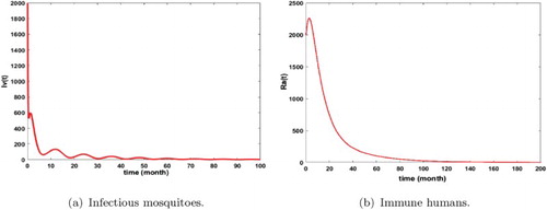
Figures 3–5 show that malaria is persistent and the system admits at least one positive periodic solution that illustrates our mathematical result of Theorem 3.14. Furthermore, we remark that the number of infected humans is very high (see Figures 3 and 4) that means that we are in the endemic region. In addition, we notice that the density of infectious non-immune is critical (see Figure 3b). As we mentioned it above, the non-immune humans are very vulnerable to malaria virus. Hence, it is very important to develop control measures in order to reduce their infectious number. These control measures can consist in fighting against immature mosquitoes proliferation (by reducing κ), avoiding contact between humans and mosquitoes (by reducing the biting rate $\beta \left(t\right)$), by protecting a proportion of non-immune through vaccination or by reducing the number of female anopheles already present in the area.

Figure 3. Distribution of infected non-immune with $d_l=4,r_v=15,d_v=3.5,b=180,{\gamma }_e=0.00054,{\gamma }_a=0.00027$ and $a_1=5,b_1=3$. The initial conditions are given by $S_e\left(0\right)=500,E_e\left(0\right)=250,I_e\left(0\right)=150,S_a\left(0\right)=1000,E_a\left(0\right)=500,I_a\left(0\right)=1000,R_a\left(0\right)=2000,S_v\left(0\right)=10,000,E_v\left(0\right)=4000,I_v\left(0\right)=2000\mathrm{and}L\left(0\right)=15,000$. We obtain $\kappa =40.6015$ and ${\mathcal{R}}_0=1.7127>1$. (a) Exposed non-immune and (b) infectious non-immune.

Figure 4. Distribution of infected semi-immune with $d_l=4,r_v=15,d_v=3.5,b=180,{\gamma }_e=0.00054,{\gamma }_a=0.00027$ and $a_1=5,b_1=3$. The initial conditions are given by $S_e\left(0\right)=500,E_e\left(0\right)=250,I_e\left(0\right)=150,S_a\left(0\right)=1000,E_a\left(0\right)=500,I_a\left(0\right)=1000,R_a\left(0\right)=2000,S_v\left(0\right)=10,000,E_v\left(0\right)=4000,I_v\left(0\right)=2000\mathrm{and}L\left(0\right)=15,000$. We obtain $\kappa =40.6015$ and ${\mathcal{R}}_0=1.7127>1$. (a) Exposed semi-immune and (b) infectious semi-immune.

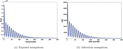
Figure 5. Distribution of infected mosquitoes with $d_l=4,r_v=15,d_v=3.5,b=180,{\gamma }_e=0.00054,{\gamma }_a=0.00027$ and $a_1=5,b_1=3$. The initial conditions are given by $S_e\left(0\right)=500,E_e\left(0\right)=250,I_e\left(0\right)=150,S_a\left(0\right)=1000,E_a\left(0\right)=500,I_a\left(0\right)=1000,R_a\left(0\right)=2000,S_v\left(0\right)=10,000,E_v\left(0\right)=4000,I_v\left(0\right)=2000,\mathrm{and}L\left(0\right)=15,000$. We obtain $\kappa =40.6015$ and ${\mathcal{R}}_0=1.7127>1$. (a) Exposed mosquitoes and (b) infectious mosquitoes.

Thus, let us assume that after some years, humans become more conscious about malaria mortality and then, develop some personal methods to avoid mosquitoes bites and also to reduce the mosquito population. By applying these measures, we obtain the following figures (Figures 6–8).

Figure 6. Distribution of infected non-immune with $a_1=3,b_1=2.5,d_l=4,d_v=7.5,b=90,{\gamma }_e={\gamma }_a=0$. The initial conditions are given by $S_e\left(0\right)=500,E_e\left(0\right)=500,I_e\left(0\right)=1000,S_a\left(0\right)=1000,E_a\left(0\right)=500,I_a\left(0\right)=1000,R_a\left(0\right)=2000,S_v\left(0\right)=10,000,E_v\left(0\right)=8000,I_v\left(0\right)=4000$ and $L\left(0\right)=15,000$. We obtain $\kappa =9.47$ and ${\mathcal{R}}_0=0.3828<1$. (a) Exposed non-immune and (a) infectious non-immune.

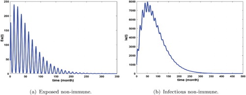
Figure 7. Distribution of semi-immune infected with $a_1=3,b_1=2.5,d_l=4,d_v=7.5,b=90,{\gamma }_e={\gamma }_a=0$. The initial conditions are given by $S_e\left(0\right)=500,E_e\left(0\right)=500,I_e\left(0\right)=1000,S_a\left(0\right)=1000,E_a\left(0\right)=500,I_a\left(0\right)=1000,R_a\left(0\right)=2000,S_v\left(0\right)=10,000,E_v\left(0\right)=8000,I_v\left(0\right)=4000$ and $L\left(0\right)=15,000$. We obtain $\kappa =9.47$ and ${\mathcal{R}}_0=0.3828<1$. (a) Exposed semi-immune and (b) infectious semi-immune.

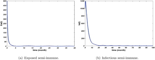
Figure 8. Distribution of infected mosquitoes with $a_1=3,b_1=2.5,d_l=4,d_v=7.5,b=90,{\gamma }_e={\gamma }_a=0$. The initial conditions are given by $S_e\left(0\right)=500,E_e\left(0\right)=500,I_e\left(0\right)=1000,S_a\left(0\right)=1000,E_a\left(0\right)=500,I_a\left(0\right)=1000,R_a\left(0\right)=2000,S_v\left(0\right)=10,000,E_v\left(0\right)=8000,I_v\left(0\right)=4000$ and $L\left(0\right)=15,000$. We obtain $\kappa =9.47$ and ${\mathcal{R}}_0=0.3828<1$. (a) Exposed mosquitoes and (b) infectious mosquitoes.

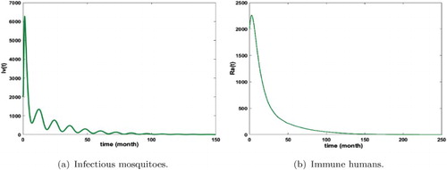
Figures 6–8 show that the solution of the system approaches the disease-free equilibrium $E^{+}$ which is globally asymptotically stable; that illustrates the result of our Theorem 3.11. Moreover, Figure 6 shows that the number of infected non-immune is rising in the short time but the disease cannot persist due to the current prevention and control measures. However, the application of these control measures must be intensified over the first 60 months of infection in order to reduce the malaria death rate for the non-immune.

Next, we perform some sensitivity analysis to determine the influence of parameters κ and $\beta \left(t\right)$ on the dynamics of malaria transmission. First, we analyse the impact of the parameter κ.

If we take the precautionary measures in the aquatic stage by reducing the parameter κ, the number of infectious humans and mosquitoes decreases rapidly as Figures 9 and 10 show it. Thus the parameter κ is very important in the dynamics of malaria transmission.

Figure 9. Distribution of infected non-immune and semi-immune with $d_l=6.5,r_v=7,d_v=7.5,b=20,{\gamma }_e={\gamma }_a=0$ and $a_1=5,b_1=3$. The initial conditions are given by $S_e\left(0\right)=500,E_e\left(0\right)=250,I_e\left(0\right)=150,S_a\left(0\right)=1000,E_a\left(0\right)=500,I_a\left(0\right)=1000,R_a\left(0\right)=2000,S_v\left(0\right)=10,000,E_v\left(0\right)=4000,I_v\left(0\right)=2000$ and $L\left(0\right)=15,000$. We get $\kappa =1.3827$ and ${\mathcal{R}}_0=0.2139<1$. (a) Infectious non-immune and (b) infectious semi-immune.

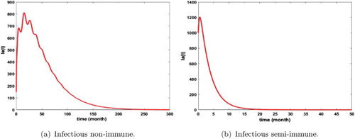
Figure 10. Distribution of infected mosquitoes and immune humans with $d_l=6.5,r_v=7,d_v=7.5,b=20,{\gamma }_e={\gamma }_a=0$ and $a_1=5,b_1=3$. The initial conditions are given by $S_e\left(0\right)=500,E_e\left(0\right)=250,I_e\left(0\right)=150,S_a\left(0\right)=1000,E_a\left(0\right)=500,I_a\left(0\right)=1000,R_a\left(0\right)=2000,S_v\left(0\right)=10,000,E_v\left(0\right)=4000,I_v\left(0\right)=2000$ and $L\left(0\right)=15,000$. We get $\kappa =1.3827$ and ${\mathcal{R}}_0=0.2139<1$. (a) Infectious mosquitoes and (b) immune humans.

Now, let us suppose that the only control measure applied by the humans consists in avoiding the bites of the mosquitoes. Let θ be the efficiency of intervention measures. By considering this prevention, we use $\hat{\beta }\left(t\right)=(1-\theta )\beta \left(t\right)$ to replace $\beta \left(t\right)$ in the model. If $\theta =0.85$, then we obtain the following results.

By applying this prevention measure, we remark that malaria disappears in the populations as shown in Figures 11 and 12. It must also be noticed that the basic reproduction decreases with this effort. In fact for the biting rate $\hat{\beta }\left(t\right)=(1-\theta )\beta \left(t\right)$, we have obtained ${\hat{\mathcal{R}}}_0=(1-\theta ){\mathcal{R}}_0$. This numerical result is consistent with our theoretical result of Proposition 3.5.

Figure 11. Distribution of infected non-immune and semi-immune with $d_l=4,r_v=15,d_v=3.5,b=180,{\gamma }_e={\gamma }_a=0$ and $a_1=5,b_1=3$. The initial conditions are given by $S_e\left(0\right)=500,E_e\left(0\right)=250,I_e\left(0\right)=150,S_a\left(0\right)=1000,E_a\left(0\right)=500,I_a\left(0\right)=1000,R_a\left(0\right)=2000,S_v\left(0\right)=10,000,E_v\left(0\right)=4000,I_v\left(0\right)=2000$ and $L\left(0\right)=15,000$. We get $\kappa =1.3827$ and ${\mathcal{R}}_0=0.2126=1.4173\times 0.15<1$. (a) Infectious non-immune and (b) infectious semi-immune.

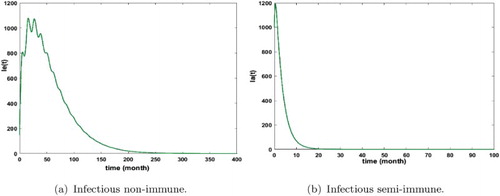
Figure 12. Distribution of infected mosquitoes and immune humans with $d_l=4,r_v=15,d_v=3.5,b=180,{\gamma }_e={\gamma }_a=0$ and $a_1=5,b_1=3$. The initial conditions are given by $S_e\left(0\right)=500,E_e\left(0\right)=250,I_e\left(0\right)=150,S_a\left(0\right)=1000,E_a\left(0\right)=500,I_a\left(0\right)=1000,R_a\left(0\right)=2000,S_v\left(0\right)=10,000,E_v\left(0\right)=4000,I_v\left(0\right)=2000$ and $L\left(0\right)=15,000$. We get $\kappa =1.3827$ and ${\mathcal{R}}_0=0.2126=1.4173\times 0.15<1$. (a) Infectious mosquitoes and (b) immune humans.

5. Conclusion

Based on the model in [10], we have formulated a mathematical model of malaria transmission with periodic biting rate and mosquitoes population structured in the heterogeneous humans host population. The basic reproduction ratios associated to the model has been determined and a new other threshold dynamics, κ, has been determined too. We have shown that κ is an important parameter which allows to control the dynamics of mosquito populations. Thus for the autonomous model, we clearly observe that basic reproduction number increases with κ. It also emerged from our study that the basic reproduction ratio is highly influenced by the biting rate. Then, these parameters could be used to fight against the disease in the populations.

Furthermore, we have determined the biological realistic disease-free equilibrium, $E^{+}$, of the model and then we have completely investigated its stability by using the Floquet theory. Indeed, we have proved that if the basic reproduction ratio, ${\mathcal{R}}_0$, is less than one, then $E^{+}$ is globally asymptotically stable and malaria dies out of the populations. Otherwise, if ${\mathcal{R}}_0$ is greater than one, the system admits at least one positive periodic solutions and malaria persists in the populations.

However, it must be noticed that our model is limited due to the following reasons:

1. seasonality is not incorporated in the evolution of immature mosquitoes, that is a mathematical simplification,

2. the immature class is not differentiated (eggs, larvae and pupae).

One can develop a more realistic model by incorporating these above assumptions and also include the investigation of the stability of positive periodic solution. Otherwise, this study could be applied to some regions with realistic data on malaria transmission that would allow to show the impact of climate on the transmission.

Disclosure statement

No potential conflict of interest was reported by the authors.

References

- J.L. Aron, Mathematical modelling of immunity to malaria, Math. Biosci. 90 (1988), pp. 385–396. doi: 10.1016/0025-5564(88)90076-4
- J.L. Aron and R.M. May, The population dynamics of malaria, in The Population Dynamics of Infectious Disease: Theory and Applications, R.M. Anderson, ed., Chapman and Hall, London, 1982, pp. 139–179.
- N. Bacaer and S. Guernaoui, The epidemic threshold of vector-borne diseases with seasonality. The case of cutaneous leishmaniasis in Chichaoua, Morocco, J. Math. Biol. 53(3) (2006), pp. 421–436. doi: 10.1007/s00285-006-0015-0
- Z. Bai and Y. Zhou, Global dynamics of an SEIRS epidemic model with periodic vaccination and seasonal contact rate, Nonlinear Anal. 13 (2012), pp. 1060–1068. doi: 10.1016/j.nonrwa.2011.02.008
- T. Berge, J.M.-S. Lubuma, G.M. Moremedi, N. Morris and R.K. Shava, A simple mathematical model for Ebola in Africa, J. Biol. Dyn. 11(1) (2017), pp. 42–74. doi: 10.1080/17513758.2016.1229817
- N. Chitnis, J.M. Cushing, and J.M. Hyman, Bifurcation analysis of a mathematical model for malaria transmission, SIAM J. Appl. Math. 67(1) (2006), pp. 24–45. doi: 10.1137/050638941
- N. Chitnis, J.M. Cushing, and J.M. Hyman, Determining important parameters in the spread of malaria through the sensitivity analysis of a mathematical model, Bull. Math. Biol. 70 (2008), pp. 1272–1296. doi: 10.1007/s11538-008-9299-0
- B. Dembele, A. Friedman, and A.A. Yakubu, Malaria model with periodic mosquito birth and death rates, J. Biol. Dyn. 3(4) (2009), pp. 430–445. doi: 10.1080/17513750802495816
- K. Dietz, L. Molineaux, and A. Thomas, A malaria model tested in the African savannah, Bull. World Health Organ. 50 (1974), pp. 347–357.
- A. Ducrot, S.B. Sirima, B. Somé, and P. Zongo, A mathematical model for malaria involving differential susceptibility, exposedness and infectivity of human host, J. Biol. Dyn. 3(6) (2009), pp. 574–598. doi: 10.1080/17513750902829393
- D.A. Ewing, C.A. Cobbold, B.V. Purse, M.A. Nunn, and S.M. white, Modelling the effect of temperature on the seasonal population dynamics of temperate mosquitoes, J. Theoret. Biol. 400 (2016), pp. 65–79. doi: 10.1016/j.jtbi.2016.04.008
- F. Forouzannia and A.B. Gumel, Mathematical analysis of an age-structured model for malaria transmission dynamics, Math. Biosci. 247 (2014), pp. 80–94. doi: 10.1016/j.mbs.2013.10.011
- J.K. Hale and S.M. Verduyn Lunel, Introduction to Functional Differential Equations, Springer, New York, 1993.
- P. Hess, Periodic–Parabolic Boundary Value Problems and Positivity, Pitman Res. Notes Math. Ser., vol. 247, Longman Scientific and Technical, Harlow, 1991.
- L.T. Keegan and J. Dushoff, Population-level effects of clinical immunity to malaria, BMC Infect. Dis. 13 (2013), 12 pages. doi: 10.1186/1471-2334-13-428
- V. Lakshmikantham, S. Leela, and A.A. Martynyuk, Stability Analysis of Nonlinear Systems, Marcel Dekker Inc., New York, Basel, 1989.
- J.P. Lasalle, The Stability of Dynamical Systems, SIAM, Philadelphia, PA, 1976.
- A.A. Lashari and G. Zaman, Global dynamics of vector-borne diseases with horizontal transmission in host population, Comput. Math. Appl. 61 (2011), pp. 745–754. doi: 10.1016/j.camwa.2010.12.018
- Y. Lou and X.-Q. Zhao, A climate-based malaria transmission model with structured vector population, SIAM J. Appl. Math. 70(6) (2010), pp. 2023–2044. doi: 10.1137/080744438
- L. Lou and X.-Q. Zhao, Modelling malaria control by introduction of larvivorous fish, Bull. Math. Biol. 73 (2011), pp. 2384–2407. doi: 10.1007/s11538-011-9628-6
- C.P. MacCormack, The human host as active agent in malaria epidemiology, Trop. Med. Parasitol. 38 (1987), pp. 233–235.
- G. Macdonald, The Epidemiology and Control of Malaria, Oxford University Press, London, 1957.
- W. McGuire, A.V.S. Hill, C.E.M. Allsopp, B.M. Greenwood, and D. Kwiatkowski, Variation in the TNF α-promoter region associated with susceptibility to cerebral malaria, Nature 371 (1994), pp. 508–511. doi: 10.1038/371508a0
- D. Moulay, M.A.A. Alaoui, and M. Cadivel, The Chikungunya disease: modelling, vector and transmission global dynamics, Math. Biosci. 229 (2011), pp. 50–63. doi: 10.1016/j.mbs.2010.10.008
- Y. Nakata and T. Kuniya, Global dynamics of a class of SEIRS epidemic models in a periodic environment, J. Math. Anal. Appl. 363 (2010), pp. 230–237. doi: 10.1016/j.jmaa.2009.08.027
- G.A. Ngwa and W.S. Shu, A mathematical model for endemic malaria with variable human and mosquito populations, Math. Comput. Model. 32 (2000), pp. 747–763. doi: 10.1016/S0895-7177(00)00169-2
- P. Olumese, Epidemiology and surveillance: changing the global picture of malaria-myth or reality?, Acta Tropica 95(3) (2005), pp. 265–269. doi: 10.1016/j.actatropica.2005.06.006
- W. Ouedraogo, B. Sangaré, and S. Traoré, Some mathematical problems arising in biological models: a predator–prey model fish-plankton, J. Appl. Math. Bioinform. 5(4) (2015), pp. 1–27.
- W. Ouedraogo, B. Sangaré, and S. Traoré, A mathematical study of cannibalism in the fish-plankton model by taking into account the catching effect, Adv. Model. Optim. 18(2) (2016), pp. 197–216.
- D. Posny and J. Wang, Modelling cholera in periodic environments, J. Biol. Dyn. 8(1) (2014), pp. 1–19. doi: 10.1080/17513758.2014.896482
- R. Ross, The Prevention of Malaria, John Murray, London, 1911.
- L. Schofield and I. Mueller, Clinical immunity to malaria, Curr. Mol. Med. 6(2) (2006), pp. 205–221. doi: 10.2174/156652406776055221
- J.P. Tian and J. Wang, Some results in Floquet theory, with application to periodic epidemic models, Appl. Anal. 2014 (2014). doi: 10.1080/00036811.2014.918606.
- B. Traoré, B. Sangaré, and S. Traoré, A mathematical model of malaria transmission with structured vector population and seasonality, J. Appl. Math. 2017 (2017), 15 pages. doi: 10.1155/2017/6754097.
- P. Van den Driessche and J. Watmough, Reproduction numbers and sub-threshold endemic equilibria for compartmental models of disease transmission, Math. Biosci. 180 (2002), pp. 29–48. doi: 10.1016/S0025-5564(02)00108-6
- W. Wang and X.-Q. Zhao, Threshold dynamics for compartmental epidemic models in periodic environments, J. Dynam. Differen. Equat. 20 (2008), pp. 699–717. doi: 10.1007/s10884-008-9111-8
- X. Wang and X.-Q. Zhao, A climate-based malaria model with the use of bed nets, J. Math. Biol. (2017). doi: 10.1007/s00285-017-1183-9.
- J. Wang, S. Gao, Y. Luo, and D. Xie, Threshold dynamics of a Huanglongbing model with logistic growth in periodic environments, Abstr. Appl. Anal. 2014 (2014), 10 pages. doi: 10.1155/2014/841367.
- World Health Organisation (WHO), Global malaria programme, World Malaria report, 2015.
- X. Xiao and X. Zou, On latencies in malaria infections and their impact on the disease dynamics, Math. Biosci. Eng. 10(2) (2013), pp. 463–481. doi: 10.3934/mbe.2013.10.463
- R. Xu, S. Zhang, and F. Zhang, Global dynamics of a delayed SEIS infectious disease model with logistic growth and saturation incidence, Math. Methods Appl. Sci. 39 (2016), pp. 3294–3308. doi: 10.1002/mma.3774
- H.M. Yang, Malaria transmission model for different levels of acquired immunity and temperature-dependent parameters (vector), Rev Saúd Públ 34 (2000), pp. 223–231. doi: 10.1590/S0034-89102000000300003
- X.-Q. Zhao, Dynamical Systems in Population Biology, Springer-Verlag, New York, 2003.