Dispersal altering local states has a limited effect on persistence of a metapopulation

ABSTRACT

Metapopulations are collections of local populations connected by dispersal. Metapopulation models often assume would-be colonists affect the states of local populations they disperse from and those they disperse to. Here, we build a new framework to include that effect and to assess the impact of dispersal. Our model predicts that a metapopulation will, in general, be found either in the state of global extinction or in the state of persistence. Our key finding is that dispersal, and the state changes associated with dispersal, have significant qualitative and quantitative effects on long-term dynamics only in a narrow range of parameter space. We conclude that life history features other than dispersal (e.g. mortality rate) have a greater influence over metapopulation persistence. We discuss the implications of our results for conservation biology, the future application of our model to the study of cooperative breeding, as well as our model's limitations.

KEYWORDS:

• Allee effect
• differential equations
• extinction–recolonization
• fragmented habitat
• tipping point

1. Introduction

Many species occupy patchy habitats, existing as a collection of local populations separated from one another in space, but linked via dispersal [6]. Understanding the dynamics of these collections of local populations, or ‘metapopulations’, is especially important to conservation efforts, as landscapes have become increasingly fragmented due to human activities [28]. Indeed, a number of mathematical models have been used to predict the conditions under which global (cf. local) extinction of metapopulations can occur.

Levins [15] provided the seminal model of metapopulation dynamics. His is a two-compartment model that classifies local populations as either empty (extinct) or occupied. It predicts that a metapopulation will persist only when the rate of local extinction is outstripped by the rate of recolonizations by dispersers from occupied areas. If, instead, the local extinction rate happens to exceed the rate of recolonization, then Levins' model predicts extinction on a global scale.

Since Levins' work [15], many more details have been incorporated into metapopulation models. Hanski [8], for example, recognized that small local populations are quite vulnerable to extinction and that emigrants from larger local populations can be a particularly important source of colonists. To capture these ideas, Hanski [8] developed a three-compartment model that subdivides occupied local populations according to their sizes (small versus large). This more elaborate model and others like it (e.g. [9]) predict that the persistence of a metapopulation and its global extinction can be alternative steady states under a limited range of conditions. In other words, a stable metapopulation could be pushed to global extinction due to a sufficiently large reduction in the population size; this represents a significant departure from the original predictions made by Levins [15].

One assumption common to metapopulation models, like those proposed by Levins and Hanski, is that dispersal from a given source population, during the course of a colonization event, does not diminish the quality of the source itself (see [1, 18, 29]). In particular, dispersal of colonists from a source population does not render the source, itself, any more vulnerable to extinction. While this assumption is convenient, it may not be reasonable, especially if local population sizes are small, or if local population dynamics highly depends on the maintenance of certain social bonds (e.g. socializing between potential mates or socializing between breeders and helpers in the nest) [14, 26].

In this paper we ask, to what extent is the persistence of a metapopulation impacted when the dispersal associated with colonization events results in a source population of diminished quality? To answer the question, we propose a simple model of a metapopulation in which local populations are made up of small numbers of individuals, with distinct social roles. We use our model to identify the conditions under which global extinction of the metapopulation can occur or be avoided. Our analysis is focused on (but not solely dedicated to) the effect of dispersal rate, as dispersal events fuel colonization in a metapopulation, and has the potential to reduce the quality of those source populations which colonists leave behind. Surprisingly, we find that the impact of dispersal, as we have modelled it, is limited. This, in turn, suggests that the standard approach is likely useful when modelling metapopulations consisting of small concentrations of social species. We discuss the implication of our findings for natural populations and their broader significance in light of model limitations.

2. Model

2.1. Preamble

In Sections 2.2–2.3.1, we build a four-compartment model of metapopulation dynamics aimed at understanding the demographic and social mechanisms that drive local extinction and recolonizations in a metapopulation. Like previous authors [8, 9], we recognize that rates of extinction and recolonization depend on the different kinds of occupied areas found in a metapopulation. Unlike previous authors, though, the way in which we classify local populations will vary according to the social status of individuals. In particular, this means that certain social roles must be filled in order for key demographic events to occur, and we expect metapopulation dynamics to change to some degree as a result.

2.2. Main assumptions

We consider a metapopulation made up of a very large number of territories. Each territory in the metapopulation can support at most two dominant individuals (as a breeding pair), with at most one non-breeding subordinate individual. In keeping with the conclusions of removal experiments with cooperatively breeding delayed dispersers [20], we assume if a subordinate happens to be found on a territory alongside only one dominant, the subordinate would immediately be recruited to the dominant class. It follows that any territory will be found in one of the four states: state 0, an empty territory; state 1, a territory with exactly one dominant and no subordinate; state 2, a territory with exactly two dominants and no subordinate; state 3, a saturated territory with exactly two dominants and one subordinate.

At time t, the state of the entire metapopulation is $n\left(t\right)=\left(n_0\right(t),n_1(t),n_2(t),n_3(t\left)\right)$, where $n_i\left(t\right)$ is the density of state-i territories. The metapopulation changes its state as a result of events associated with demographic processes, including mortality, birth and dispersal. We discuss each demographic process, in turn, below.

2.3. Demographic processes

2.3.1. Mortality

Each individual suffers mortality at rate of $\mu >0$ per unit time. Mortality of individuals on a state-i>0 territory implies a transition to state i−1 (Figure 1a). As is clear from Figure 1(a), the directions of arrows related to mortality rate are all pointing to left, which implies increasing mortality will promote global extinction.

Figure 1. Transitions among territory states. The demographic processes lead to state transitions: (a) due to mortality, (b) due to birth, (c) due to dispersal. Note that arrows associated with mortality are all pointing to the left, arrows associated with birth are all pointing to the right, but arrows associated with dispersal are not of the same direction.

2.3.2. Birth

A pair of dominant individuals gives birth at rate $\lambda >0$ per unit time. If the dominant pair inhabits a state-2 territory, any newborn they produce immediately becomes a subordinate on the same territory. In this case, the state-2 territory transitions to state 3 (Figure 1b). While it is true that birth events occur on state-3 territories, newborns produced on those saturated territories are assumed to migrate; the associated state transitions are discussed later. In Figure 1(b,c), the directions of arrows due to birth are all pointing right, meaning that birth promotes persistence of metapopulation.

2.3.3. Dispersal

A subordinate individual emigrates from a state-3 territory at rate $\delta >0$ per unit time. In addition, individuals born on a state-3 territory are assumed to emigrate at the moment of their birth (equivalently, the incumbent subordinate migrates the moment the birth event takes place and the newborn remains). Upon leaving a state-3 territory, an emigrant travels to a new territory, chosen uniformly at random, in an attempt to fill a dominant vacancy. If an emigrant chooses to travel to a territory with no dominant vacancy, that emigrant is assumed to die. In this way, dispersal is risky. In Figure 1(c), arrows associated with dispersal are not of the same direction, so the effect of dispersal on persistence of metapopulation is not obvious. This is indeed the basic motivation of this paper.

Our model of dispersal is consistent with the social behaviours of certain cooperatively breeding species who reject non-kin when these outsiders attempt to join their groups. Broadly speaking, the rejection of non-kin is predicted to occur whenever the group in question is in its most productive state (e.g. groups that are in state 2) [22]. Our model of dispersal also leads to kin-based social groups which is consistent with a number of studies of avian cooperative breeding (see [10]). Of course, allowing only kin to join certain social groups does lead to inbreeding, but certain social species are known to tolerate inbreeding to some degree [19].

Overall, dispersal contributes to the transitions of territories from state 3 to state 2, from state 1 to state 2, and from state 0 to state 1 (Figure 1c). Importantly, transitions from state 3 to state 2 at one locale can be linked to changes from state 1 to state 2, or 0 to 1, at another locale. In this way, our model differs from earlier ones [8, 9] that treat the degradation in quality of local environments as independent events.

2.4. Dynamics

2.4.1. ODE system

Combining the processes given in Figure 1(a–c), we obtain the following ODEs for $n_0$ to $n_3$, respectively: (1) $\begin{array}{rl}\frac{\mathrm{d}{n}_0}{\mathrm{d}t}& =\mu n_1-\frac{n_0}{N}(\lambda +\delta )n_3,\\ \frac{\mathrm{d}{n}_1}{\mathrm{d}t}& =-\mu n_1+\frac{n_0}{N}(\lambda +\delta )n_3+2\mu n_2-\frac{n_1}{N}(\lambda +\delta )n_3,\\ \frac{\mathrm{d}{n}_2}{\mathrm{d}t}& =(3\mu +\delta )n_3-\lambda n_2-2\mu n_0+\frac{n_1}{N}(\lambda +\delta )n_3,\\ \frac{\mathrm{d}{n}_3}{\mathrm{d}t}& =-(3\mu +\delta )n_3+\lambda n_2,\end{array}$(1) where the total number of territories is $N=n_0+n_1+n_2+n_3$. Note that $\mathrm{d}N/\mathrm{d}t=0$, so the total density is a constant. We then non-dimensionalize the system (1(1) $\begin{array}{rl}\frac{\mathrm{d}{n}_0}{\mathrm{d}t}& =\mu n_1-\frac{n_0}{N}(\lambda +\delta )n_3,\\ \frac{\mathrm{d}{n}_1}{\mathrm{d}t}& =-\mu n_1+\frac{n_0}{N}(\lambda +\delta )n_3+2\mu n_2-\frac{n_1}{N}(\lambda +\delta )n_3,\\ \frac{\mathrm{d}{n}_2}{\mathrm{d}t}& =(3\mu +\delta )n_3-\lambda n_2-2\mu n_0+\frac{n_1}{N}(\lambda +\delta )n_3,\\ \frac{\mathrm{d}{n}_3}{\mathrm{d}t}& =-(3\mu +\delta )n_3+\lambda n_2,\end{array}$(1) ) using $w=n_0/N,x=n_1/N,y=n_2/N,z=n_3/N,\tau =t\lambda$, so it becomes $\begin{array}{rl}\dot{w}& =mx-(1+d)wz,\\ \dot{x}& =-mx+(1+d)wz+2my-(1+d)xz,\\ \dot{y}& =-y+(3m+d)z-2my+(1+d)xz,\\ \dot{z}& =y-(3m+d)z,\end{array}$ where $m=\mu /\lambda$ is the non-dimensionalized mortality rate of an individual, $d=\delta /\lambda$ is the non-dimensionalized dispersal rate of a subordinate individual and dots denote derivatives with respect to τ. Note that w, x, y, z are fractions of territories in a given state (state 0, state 1, state 2, state 3, respectively) and that τ marks time in terms of birth events ($\tau =1$ when $t=1/\lambda$). Using w+x+y+z=1, the previous system can be reduced to our final three-dimensional system (2) $\begin{array}{rl}\dot{x}& =-mx+(1+d)(1-x-y-z)z+2my-(1+d)xz,\\ \dot{y}& =-y+(3m+d)z-2my+(1+d)xz,\\ \dot{z}& =y-(3m+d)z.\end{array}$(2) We present our analysis of the system (2(2) $\begin{array}{rl}\dot{x}& =-mx+(1+d)(1-x-y-z)z+2my-(1+d)xz,\\ \dot{y}& =-y+(3m+d)z-2my+(1+d)xz,\\ \dot{z}& =y-(3m+d)z.\end{array}$(2) ) here, but symbolic and numerical calculations are also outlined in the computer code included as supplemental files.

2.4.2. Forward invariance of the system

Before exploring further properties of the system, we present a proposition that serves, for now, as a check on correctness of system (2(2) $\begin{array}{rl}\dot{x}& =-mx+(1+d)(1-x-y-z)z+2my-(1+d)xz,\\ \dot{y}& =-y+(3m+d)z-2my+(1+d)xz,\\ \dot{z}& =y-(3m+d)z.\end{array}$(2) ). Of course, solutions that track fractions of some population ought to stay bounded within the simplex. Proposition 2.1 shows that this is true of solutions to the ODEs proposed above.

Proposition 2.1

Solutions to (2(2) $\begin{array}{rl}\dot{x}& =-mx+(1+d)(1-x-y-z)z+2my-(1+d)xz,\\ \dot{y}& =-y+(3m+d)z-2my+(1+d)xz,\\ \dot{z}& =y-(3m+d)z.\end{array}$(2) ), paired with an initial condition, remain in the region $C=\left\{\right(x,y,z)|x+y+z\le 1,0\le x,y,z\le 1\},$ as long as the initial condition is in the region C.

Proof.

We need only check that the dot product between the inward-pointing normal to C and the vector field $(\dot{x},\dot{y},\dot{z})$ is positive on boundaries of C.

Note that there are four sets that make up boundaries of C (its ‘faces’). Those includes x+y+z=1, x=0, y=0 and z=0. On the face x+y+z=1, the normal vector is $(-1,-1,-1)$, which is pointing inward the region C. Then, we can get $(-1,-1,-1)\cdot (\dot{x},\dot{y},\dot{z})=mx\ge 0$, which means the flow on the edge cannot cross the boundary. On the face x=0, the normal vector is $(1,0,0)$ pointing inward, and $(1,0,0)\cdot (\dot{x},\dot{y},\dot{z}){|}_{x=0}=z(1-y-z)(d+1)+2my\ge 0$. Similar proof can be obtained on the other two faces y=0 and z=0.

3. Results

Focusing on system (2(2) $\begin{array}{rl}\dot{x}& =-mx+(1+d)(1-x-y-z)z+2my-(1+d)xz,\\ \dot{y}& =-y+(3m+d)z-2my+(1+d)xz,\\ \dot{z}& =y-(3m+d)z.\end{array}$(2) ), it is obvious that there is an extinction equilibrium (when $(x,y,z)=(0,0,0)$) that always exists. As the reader will see, two addition (positive) equilibria may also exist, depending on the demographic parameters. We will investigate the stability of the extinction equilibrium in Section 3.1, and the existence and the stability of positive equilibria will be discussed in Section 3.2. We also study the effect of changing d and m on the persistence of metapopulation in Section 3.2.

3.1. Extinction equilibrium

The vector $E_0=(x,y,z)=(0,0,0)$ is an equilibrium solution to system (2(2) $\begin{array}{rl}\dot{x}& =-mx+(1+d)(1-x-y-z)z+2my-(1+d)xz,\\ \dot{y}& =-y+(3m+d)z-2my+(1+d)xz,\\ \dot{z}& =y-(3m+d)z.\end{array}$(2) ). At this equilibrium, all of the territories are at state 0, so the species is absent from the metapopulation, and we call $E_0$ the ‘extinction equilibrium’. To verify that the equilibrium is locally asymptotically stable (LAS), we consider the $3\times 3$ Jacobian matrix, constructed by linearizing (2(2) $\begin{array}{rl}\dot{x}& =-mx+(1+d)(1-x-y-z)z+2my-(1+d)xz,\\ \dot{y}& =-y+(3m+d)z-2my+(1+d)xz,\\ \dot{z}& =y-(3m+d)z.\end{array}$(2) ) about $E_0$: $J_{E_0}=\left[\begin{array}{ccc}-m& 2m& d+1\\ 0& -2m-1& d+3m\\ 0& 1& -(d+3m)\end{array}\right].$ We can see one of the eigenvalues of $J_{E_0}$ is $-m<0$. The sign of real part of the other two eigenvalues depends on the trace and determinant of a $2\times 2$ matrix located in the lower right corner of $J_{E_0}$. The trace of $J_{E_0}$ is $-2m-1-(d+3m)<0$, and its determinant is $2(d+3m)m>0$, so the remaining two eigenvalues both have negative real part. It follows, from the Routh–Hurwitz criteria (see, e.g. [4]), that all of the eigenvalues of $J_{E_0}$ have negative real parts, so the extinction equilibrium $E_0$ is LAS. Whether $E_0$ is globally asymptotically stable depends on the parameters, because there could be other equilibria. Hence, we have only the following proposition, in general.

Proposition 3.1

For system (2(2) $\begin{array}{rl}\dot{x}& =-mx+(1+d)(1-x-y-z)z+2my-(1+d)xz,\\ \dot{y}& =-y+(3m+d)z-2my+(1+d)xz,\\ \dot{z}& =y-(3m+d)z.\end{array}$(2) ), there always exists a trivial extinction equilibrium, which is locally asymptotically stable.

Proposition 3.1 distinguishes our model from earlier ones [8, 9] in that the extinction equilibrium in our model is stable for all parameters, not a subset of all parameters. We discuss this proposition in the final section.

3.2. Positive equilibria

If z=0, then the extinction equilibrium is the only steady-state solution to (2(2) $\begin{array}{rl}\dot{x}& =-mx+(1+d)(1-x-y-z)z+2my-(1+d)xz,\\ \dot{y}& =-y+(3m+d)z-2my+(1+d)xz,\\ \dot{z}& =y-(3m+d)z.\end{array}$(2) ). Biologically speaking, z=0 means there is no territory with a breeding pair and a subordinate, so there are not enough offspring being produced and subordinates to fill vacancies, which leads to the extinction of the population. When investigating the possibility of positive equilibria, then we ought to consider $z\ne 0$ only.

If $z\ne 0$, then a positive equilibrium, if it exists, satisfies $\begin{array}{rl}-mx+(1+d)(1-x-y-z)z+2my-(1+d)xz& =0,\\ -y+(d+3m)z-2my+(1+d)xz& =0,\\ y-(d+3m)z& =0,\end{array}$ which is equivalent to (3) $\begin{array}{rl}-mx+(1+d)(1-x-y-z)z& =0,\\ -2my+(1+d)xz& =0,\\ y-(d+3m)z& =0.\end{array}$(3) Using the last two equations in (3(3) $\begin{array}{rl}-mx+(1+d)(1-x-y-z)z& =0,\\ -2my+(1+d)xz& =0,\\ y-(d+3m)z& =0.\end{array}$(3) ), we can express x and y in terms of z: (4) $x=\frac{2(d+3m)m}{1+d},y=(d+3m)z.$(4) Substituting (4(4) $x=\frac{2(d+3m)m}{1+d},y=(d+3m)z.$(4) ) into the first equation in (3(3) $\begin{array}{rl}-mx+(1+d)(1-x-y-z)z& =0,\\ -2my+(1+d)xz& =0,\\ y-(d+3m)z& =0.\end{array}$(3) ), we obtain a quadratic equation for the equilibrium density of state-3 territories z. This can be solved to get (5) $z_{\pm }=\frac{d+1-2(d+3m)m\pm \sqrt{D}}{2(d+3m+1)(d+1)},$(5) where (6) $D=(d+1-2(d+3m)m{)}^2-8m^2(d+3m\left)\right(d+3m+1)$(6) is the discriminant. Of course, when D>0, we have $0<z_{\pm }<1$ and the corresponding two positive equilibria using Equations (4(4) $x=\frac{2(d+3m)m}{1+d},y=(d+3m)z.$(4) ) and (5(5) $z_{\pm }=\frac{d+1-2(d+3m)m\pm \sqrt{D}}{2(d+3m+1)(d+1)},$(5) ). We denote the two positive equilibria as $E_{-}=(x,y(z_{-}),z_{-})$ and $E_{+}=(x,y(z_{+}),z_{+})$, respectively. When D<0, there is no solution with real values. When D=0, the two equilibria coincide, i.e. $z_{+}=z_{-}=(d+1-2(d+3m\left)m\right)/\left(2\right(d+3m+1\left)\right(d+1\left)\right)$, and we will not concern ourselves with stability. Indeed, it is the case D>0 that concerns us in the proposition that follows.

Proposition 3.2

System (2(2) $\begin{array}{rl}\dot{x}& =-mx+(1+d)(1-x-y-z)z+2my-(1+d)xz,\\ \dot{y}& =-y+(3m+d)z-2my+(1+d)xz,\\ \dot{z}& =y-(3m+d)z.\end{array}$(2) ) has two positive equilibria if and only if D>0 is satisfied. The equilibrium corresponding to a larger population size is locally asymptotically stable; the other is unstable.

Proof.

The existence of two positive equilibria, when D>0, has been shown above, so we only need to examine their stability. The claims about local stability can be proven by investigating the linearization of the system (2(2) $\begin{array}{rl}\dot{x}& =-mx+(1+d)(1-x-y-z)z+2my-(1+d)xz,\\ \dot{y}& =-y+(3m+d)z-2my+(1+d)xz,\\ \dot{z}& =y-(3m+d)z.\end{array}$(2) ) about the corresponding positive equilibrium. The characteristic polynomial associated with the operator from the aforementioned linearization is $f\left(\nu \right)=\left|\begin{array}{ccc}\nu +2(d+1)z+m& (d+1)z-2m& (d+1)(2x+y+2z-1)\\ -(d+1)z& \nu +2m+1& -(d+1)x-(d+3m)\\ 0& -1& \nu +(d+3m)\end{array}\right|.$ Using Equation (4(4) $x=\frac{2(d+3m)m}{1+d},y=(d+3m)z.$(4) ), we simplify the polynomial and get (7) $\begin{array}{rl}f\left(\nu \right)& ={\nu }^3+\underset{=k_1}{\underbrace{\left[2\right(d+1)z+(d+3m)+3m+1]}}{\nu }^2\\ & +\underset{=k_2}{\underbrace{\left[\right(d+1{)}^2{z}^2+2(d+1)(d+4m+1)z+m(d+5m+1)]}}\nu \\ & +\underset{=k_3}{\underbrace{\left[2\right(d+1\left)z\right((d+1)(d+3m+1)z+\left(2\right(d+3m)m-(d+1\left)\right)\left)\right]}}.\end{array}$(7) If the real parts of each of the roots of the polynomial are negative, then the equilibrium is locally asymptotically stable. The Routh–Hurwitz criteria for polynomials like (7(7) $\begin{array}{rl}f\left(\nu \right)& ={\nu }^3+\underset{=k_1}{\underbrace{\left[2\right(d+1)z+(d+3m)+3m+1]}}{\nu }^2\\ & +\underset{=k_2}{\underbrace{\left[\right(d+1{)}^2{z}^2+2(d+1)(d+4m+1)z+m(d+5m+1)]}}\nu \\ & +\underset{=k_3}{\underbrace{\left[2\right(d+1\left)z\right((d+1)(d+3m+1)z+\left(2\right(d+3m)m-(d+1\left)\right)\left)\right]}}.\end{array}$(7) ) declares that all the roots of the equation have negative real parts if and only if each of $k_1>0,k_3>0$ and $k_1{k}_2-k_3>0$ hold. For our polynomial, the three conditions are (8a) $2(d+1)z+(d+3m)+3m+1>0,$(8a) (8b) $\begin{array}{rl}& \left[2(d+1)z+(d+3m)+3m+1\right]\left[\right(d+1{)}^2{z}^2+2(d+1)(d+4m+1)z+m(d+5m+1)]\\ & -\left[2(d+1)z\left(\right(d+1\left)\right(d+3m+1)z+(2(d+3m)m-(d+1)\left)\right)\right]>0,\end{array}$(8b) (8c) $2(d+1)z\left[(d+1)(d+3m+1)z+\left(2\right(d+3m)m-(d+1\left)\right)\right]>0.$(8c) It is obvious that the condition (8a(8a) $2(d+1)z+(d+3m)+3m+1>0,$(8a) ) holds for all z>0, because all parameters d,m are positive. To prove condition (8c(8c) $2(d+1)z\left[(d+1)(d+3m+1)z+\left(2\right(d+3m)m-(d+1\left)\right)\right]>0.$(8c) ) holds, we can partially expand the left-hand side of the expression to get $\begin{array}{rl}& 2{\left(d+1\right)}^3{z}^3+\left(3(d+3m)+7m+3\right){\left(d+1\right)}^2{z}^2\\ & +\left(d+10m^2+2\left(4(d+3m)+5\right)m+2{(d+3m)}^2+4(d+3m)+3\right)\left(d+1\right)z\\ & +m\left((d+3m)+3m+1\right)\left((d+3m)+2m+1\right).\end{array}$ This is also positive for positive parameters d,m and non-negative variable z. Since $z_{\pm }>0$, it is true that both equilibria satisfy the condition (8a(8a) $2(d+1)z+(d+3m)+3m+1>0,$(8a) ) and condition (8c(8c) $2(d+1)z\left[(d+1)(d+3m+1)z+\left(2\right(d+3m)m-(d+1\left)\right)\right]>0.$(8c) ).

As for the condition (8c(8c) $2(d+1)z\left[(d+1)(d+3m+1)z+\left(2\right(d+3m)m-(d+1\left)\right)\right]>0.$(8c) ), it is equivalent to $(d+1)(d+3m+1)z+\left(2\right(d+3m)m-(d+1\left)\right)>0,$ or (9) $z>\frac{d+1-2(d+3m)m}{(d+1)(d+3m+1)}.$(9) We then have $\begin{array}{rl}{z}_{+}& =\frac{d+1-2(d+3m)m+\sqrt{D}}{2(d+3m+1)(d+1)}\\ & >\frac{d+1-2(d+3m)m}{2(d+3m+1)(d+1)}>\frac{d+1-2(d+3m)m-\sqrt{D}}{2(d+3m+1)(d+1)}=z_{-},\end{array}$ for D>0. So, for $z=z_{+}$, the condition (8c(8c) $2(d+1)z\left[(d+1)(d+3m+1)z+\left(2\right(d+3m)m-(d+1\left)\right)\right]>0.$(8c) ) holds, and the equilibrium associated with $z=z_{+}$ is LAS. For $z=z_{-}$, the condition (8c(8c) $2(d+1)z\left[(d+1)(d+3m+1)z+\left(2\right(d+3m)m-(d+1\left)\right)\right]>0.$(8c) ) fails as the reverse inequality, so the equilibrium associated with $z_{-}$ is unstable.

The consequences of Propositions 3.1 and 3.2 for the bifurcation of solutions to system (2(2) $\begin{array}{rl}\dot{x}& =-mx+(1+d)(1-x-y-z)z+2my-(1+d)xz,\\ \dot{y}& =-y+(3m+d)z-2my+(1+d)xz,\\ \dot{z}& =y-(3m+d)z.\end{array}$(2) ) are illustrated in Figure 2.

Figure 2. The bifurcation diagram of system (2(2) $\begin{array}{rl}\dot{x}& =-mx+(1+d)(1-x-y-z)z+2my-(1+d)xz,\\ \dot{y}& =-y+(3m+d)z-2my+(1+d)xz,\\ \dot{z}& =y-(3m+d)z.\end{array}$(2) ). The equilibrium proportions of state-3 territories, generically denoted as z, change with increasing discriminant D, as does their respective stability properties. In the figure, z=0 and $z_{+}$ correspond to locally stable equilibria $E_0$ and $E_{+}$, respectively, and are shown in solid lines. The value $z_{-}$ corresponds to the locally unstable equilibrium, $E_{-}$, is shown as the dotted line. We obtain the corresponding values of the discriminant D and $z_{\pm }$, by fixing the dispersal rate d as a constant, and changing the mortality rate m.

In Figure 2, we use the discriminant D as a bifurcation parameter. If D<0, we see that there is only one equilibrium, the extinction equilibrium, $E_0$, and it is stable. At D=0 a bifurcation occurs, and for D>0 we see the appearance of a stable equilibrium (denoted $E_{+}$ in Figure 2) corresponding to $z_{+}$ and an unstable equilibrium (denoted $E_{-}$ in Figure 2) corresponding to $z_{-}$. In biological terms, D=0 can be viewed as a ‘tipping point’ [21, sensu] since any demographic or life history changes that take D below zero also result in guaranteed extinction of the metapopulation.

At the tipping point D=0, itself, the characteristic polynomial (7(7) $\begin{array}{rl}f\left(\nu \right)& ={\nu }^3+\underset{=k_1}{\underbrace{\left[2\right(d+1)z+(d+3m)+3m+1]}}{\nu }^2\\ & +\underset{=k_2}{\underbrace{\left[\right(d+1{)}^2{z}^2+2(d+1)(d+4m+1)z+m(d+5m+1)]}}\nu \\ & +\underset{=k_3}{\underbrace{\left[2\right(d+1\left)z\right((d+1)(d+3m+1)z+\left(2\right(d+3m)m-(d+1\left)\right)\left)\right]}}.\end{array}$(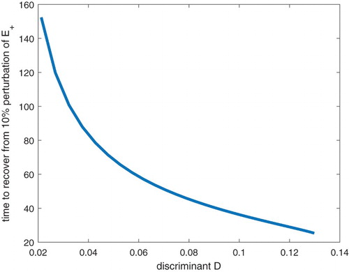7) ) has a zero root. By continuity, this means that near-equilibrium dynamics close to the tipping point will be dominated by small eigenvalues. Therefore we expect to see a critical slowing down for population density to get back to the stable positive equilibrium after perturbation [21]. In turn, that critical slowing down implies that, in a natural setting, perturbations of the stable equilibrium would take longer to be corrected in those systems nearer to D=0 (Figure 3), which might be an early sign that efforts to conserve the metapopulation need to be increased.

Figure 3. The relationship between the time required to recover from a $10\mathrm{\%}$ perturbation from $E_{+}$ and the discriminant D. We fix the mortality rate m as a constant, and change the dispersal rate d, to obtain corresponding values of correction time and the discriminant D. Other computational details included in supplementary files.

Close to this tipping point D=0, we observe how the metapopulation can be affected by changing mortality rate and dispersal rate. For any given value of d, increasing mortality rate m will eventually lead the metapopulation to lose its stable positive equilibrium and go extinct, because $\mathrm{\partial }D/\mathrm{\partial }m<0$ for all m and d (Figure 4 when d is a constant).

Figure 4. (a) The relationship between the sign of the discriminant D and parameters d and m. The solid curve is the contour of $D(d,m)=0$. (b) The relationship between the equilibria (represented by equilibrium value of state-3 territories, $z_{\pm }$) and parameters and m, for various values of d.

For given values of m, increasing dispersal rate d can have mixed effects on the metapopulation. Three cases are summarized as follows (Figure 4). First, if $m<m_1=(\sqrt{2}-1)/2$, then changing D does not change the sign of D, because $\mathrm{\partial }D/\mathrm{\partial }d>0$ for all d>0 with $D(m,0)>0$. So the metapopulation always has a stable positive equilibrium, and it always has a chance to persist. Second, if m is between $m_1$ and $m_0$, then increasing d will eventually push the metapopulation to extinction because $\mathrm{\partial }D/\mathrm{\partial }d{|}_{D(d,m)=0}<0$. Third, if $m>m_0$, increasing d will not change the sign of D, which stays negative. Overall, $m_0-m_1$ gives the range of mortality rates over which we observe the negative effect of increasing d. Importantly, this range is small relative to the width of the region to the left of $m_1$, where increasing d does not affect the existence of $E_{+}$ (Figure 4). In sum, for the vast majority of parameter combinations, changing d does not bring populations closer to D=0, and so does not bring them closer to extinction.

Figure 2 also suggests that there is a second kind of tipping point predicted by our model, when the metapopulation is to the right of the bifurcation (D>0 in Figure 2). Specifically, the tipping point is a set (possibly a surface) that separates the basins of attraction for $E_0$ and $E_{+}$, respectively, on which we find $E_{-}$ (Figure 5).

Figure 5. The boundary between the basin of attraction for $E_0$ and that for $E_{+}$. The boundary itself is shown as a dotted blue surface. Equilibria $E_0$ and $E_{+}$ are shown as the black dot and the red dot, respectively. The unstable equilibrium $E_{-}$ is shown as the large blue dot on the boundary surface.

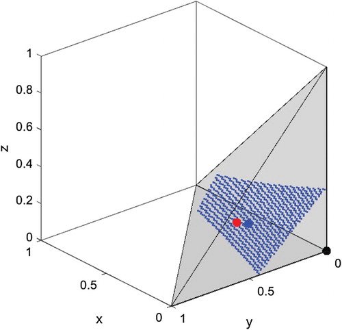
This second kind of tipping point has been identified in other metapopulation models, and is linked to an Allee effect, i.e. negative population growth below some density threshold [1, 18]. In our model, the tipping point can be avoided in stable populations provided perturbations remain inside the basin of attraction for $E_{+}$ (region above the boundary surface in Figure 5).

Unfortunately, neither Figure 2 nor 5 can clarify the effect of changing d on the volume of basin of attraction for $E_{+}$. To take a more detailed look at the second kind of tipping point, we investigate the volume of the basin of attraction of $E_{+}$ and how it is affected by the change of demographic parameters d given m. Since obtaining an explicit expression of the boundary surface is not possible, we introduce a numerical way to measure the fraction of the volume of the basin of attraction of $E_{+}$ in the phase space C. First, we generate ${10}^5$ random triples $(x_0,y_0,z_0)$ in $[0,1{]}^3$ and use those satisfying $x_0+y_0+z_0\le 0$ as initial conditions. From the initial conditions, we solve (2(2) $\begin{array}{rl}\dot{x}& =-mx+(1+d)(1-x-y-z)z+2my-(1+d)xz,\\ \dot{y}& =-y+(3m+d)z-2my+(1+d)xz,\\ \dot{z}& =y-(3m+d)z.\end{array}$(2) ) using the Runge–Kutta–Fehlberg (RKF) method (see supplementary information). If the solution ends up in a small neighbourhood surrounding $E_{+}$ (resp. $E_0$), then the corresponding initial condition is assigned to the basin of attraction for $E_{+}$ (resp. $E_0$). We utilize Proposition 2.1 in numerical simulations: if solutions leave the region C, we attribute their departure to numerical errors and discard them. We divide the number of initial points ending up in the neighbourhood of $E_{+}$ ($E_0$, respectively) by the total number of valid initial points, and get the fraction of C that corresponds to the basin of attraction for each of $E_{+}$ and $E_0$. We are interested in the persistence of metapopulation, so we report the fraction of C that corresponds to the basin of attraction for $E_{+}$ in Figure 6.

Figure 6. (a) Relationship between the volume of basin of attraction for the positive stable equilibrium $E_{+}$ and dispersal rate d and morality rate m (simulated results). (b) Five examples of the relationships in part (a) with specified values of m show the decreasing trend of the volume of basin of attraction, when increasing d.

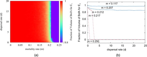
Numerical solution of (2(2) $\begin{array}{rl}\dot{x}& =-mx+(1+d)(1-x-y-z)z+2my-(1+d)xz,\\ \dot{y}& =-y+(3m+d)z-2my+(1+d)xz,\\ \dot{z}& =y-(3m+d)z.\end{array}$(2) ) reveals a negative relationship between the value of d>0 and the volume of the basin of attraction of $E_{+}$ (Figure 6b). Increasing dispersal rate only changes the volume of basin of attraction of $E_{+}$ dramatically in a narrow range where bifurcation occurs. It is obvious that for most of parameter space, change in dispersal rate does not significantly affect the metapopulation dynamics (the regions with constant mortality rate remain the same colour when changing dispersal rate in most of Figure 6a).

4. Discussion

Metapopulation models describe how a balance between occupied and unoccupied habitat patches is, or is not, maintained by colonization and extinction events. Most of these models assume that would-be colonists do not alter the state of the patch they leave upon departure (see [1, 8, 9, 15, 18, 29]). When habitat patches are occupied by small numbers of individuals, however, dispersal by would-be colonists could leave a patch more susceptible to extinction associated with random events. If dispersal by individuals also disrupts social roles, then departure by colonists could have an even greater negative effect on the patches they leave behind.

In this paper, we use a mathematical model to investigate how dispersal-associated state changes in a metapopulation might impact its dynamics. In particular, we are interested in extinction. In contrast to previous work [8, 9], our analysis shows that the extinction equilibrium is stable for all possible demographic conditions. The difference between our model and previous ones is due to the fact that successful colonization is a ‘second-order’ process. In our model, one colonist must be followed soon after by a second before reproduction can occur, and at low population densities this is very unlikely. Earlier models ignore the social complexities of the mating process, thereby allowing the extinction equilibrium to lose stability, under certain conditions.

Our model assumes local populations (patches) are occupied by small numbers of individuals, with distinct social roles. Admittedly, we make rigid assumptions about the way in which local populations are structured. However, our assumptions should emphasize, if not maximize, the influence of dispersal-related state changes on global dynamics. That said, our model predicts that dispersal from occupied patches by socially subordinate individuals has limited impact on the global persistence of a metapopulation. While it is true that changing dispersal could, in some cases, tip the population toward (or away from) global extinction or make the population less robust in the face of perturbation, those cases represented only a very narrow range of parameter space. Our principal conclusion, then, is that dispersal-related state changes do not impact significantly on the long-term persistence of the metapopulation as a whole. This does not mean that small local populations or social ties among neighbours play no role in metapopulation dynamics; rather, it means that the influence of dispersal is not as strong as the influence of other demographic processes like mortality.

The role played by dispersal in metapopulation dynamics is relevant to an on-going debate among conservation biologists about the use of dispersal corridors to prevent extinction [3, 5, 25]. On one hand, corridors are considered to be effective management tools because the movement they promote stems inbreeding depression and is thought to reduce size variation among small local populations [23]. On the other hand, dispersal corridors may promote the spread of disease, introduce additional sources of mortality and may otherwise be ineffective depending on the natural history of the species at risk [12, 24]. The resolution of the debate over the efficacy of dispersal corridors also has economic implications, as the construction of these corridors can cost several millions of dollars to establish and maintain [16, 25]. Insofar as conservation biologists are concerned with dispersal corridors impacting on the social lives of small local populations, our model's predictions can contribute to the resolution of the debate. In particular, we predict that any negative effects of dispersal would be observed in only a narrow range of background biological conditions. Provided corridors are used, our model indicates that concerns over the rate at which they are travelled are secondary to concerns about birth and mortality rates. Of course, movement corridors may benefit the metapopulation in some cases, and the demographic parameters should be monitored to assess the effectiveness of corridors. In that way, it is possible to reduce the cost–benefit ratio of investment for conservation.

Our conclusions should be tempered by the fact that our model, like all models, makes certain key assumptions. Perhaps the most important assumption we make is that demographic rates fixed. Although this assumption is common in models of population dynamics, generally speaking, longevity and birth rates are understood as being shaped by selection [2]. Moreover, dispersal rate is expected to evolve [17], especially in response to social-evolutionary pressure imposed by small local population [7, 13]. We have already identified a role for dispersal in a narrow range of parameter space. It is important to note that, if demographic rates were allowed to evolve, what seems to be a narrow range of parameter space could turn out to be exactly where selection on demographic traits pushes the metapopulation. Future work investigating the so-called ‘eco-evolutionary dynamics’ in metapopulations will resolve this issue.

One criticism that could be levied against our model has to do with the rather simplistic nature of the social interactions it incorporates. We have suggested, above, that our model captures certain elements of the biology of cooperative (i.e. communal) breeders. Certain other elements, though, are missing.

Before we launch into the missing elements, let us remind the reader that we have focused on relationships between mates, as well as on dominant–subordinate interactions among immediate neighbours. Most notably, subordinates can inherit dominant positions from their reproductively active parents. This fits well with the goals of the paper: given the uncertainty associated with dispersal, departures by would-be colonists could definitely disrupt the productivity of patches they leave behind. The feature also fits with certain hypothesized incentives for cooperative breeding [27].

Despite the various positives, what makes our model a poor one for understanding cooperative breeding is that cooperation itself is missing. Subordinates in our model do nothing to change the birth or mortality rates of dominants, whereas these rates are observed to change in natural cooperatively breeding populations [11]. Had our model incorporated richer social structure our conclusions may have changed – especially since cooperative interactions would be yet another thing for dispersal to disrupt. Importantly, incorporation of richer social structure would have (will) complicate the model, and so future work that seeks to resolve this issue must also find a way to cope with the perennial trade-off between realism and tractability.

Acknowledgments

Comments provided by an anonymous reviewer improve an earlier draft of the work.

Disclosure statement

The authors have no conflicts of interest.

ORCID

Jingjing Xu http://orcid.org/0000-0003-0581-0697

Geoff Wild http://orcid.org/0000-0001-7821-7304

Additional information

Funding

This work was supported by the Natural Sciences and Engineering Research Council of Canada under Discovery Grant number 549848.

References

- P. Amarasekare, Allee effects in metapopulation dynamics, Am. Nat. 152 (1998), pp. 298–302. doi: 10.1086/286169
- M. Begon, J.L. Harper, and C.R. Townsend, et al., Ecology. Individuals, Populations and Communities, Blackwell Scientific Publications, Boston, 1986.
- P. Beier and R.F. Noss, Do habitat corridors provide connectivity?, Conserv. Biol. 12 (1998), pp. 1241–1252. doi: 10.1046/j.1523-1739.1998.98036.x
- N. Britton, Essential Mathematical Biology, Springer Science & Business Media, London, 2012.
- L. Gilbert-Norton, R. Wilson, J.R. Stevens, and K.H. Beard, A meta-analytic review of corridor effectiveness, Conserv. Biol. 24 (2010), pp. 660–668. doi: 10.1111/j.1523-1739.2010.01450.x
- M. Gilpin, Metapopulation Dynamics: Empirical and Theoretical Investigations, Academic Press, London, 2012.
- W.D. Hamilton and R.M. May, Dispersal in stable habitats, Nature 269 (1977), pp. 578–581. doi: 10.1038/269578a0
- I. Hanski, Single-species spatial dynamics may contribute to long-term rarity and commonness, Ecology 66 (1985), pp. 335–343. doi: 10.2307/1940383
- A. Hastings, Structured models of metapopulation dynamics, Biol. J. Linnean Soc. 42 (1991), pp. 57–71. doi: 10.1111/j.1095-8312.1991.tb00551.x
- B.J. Hatchwell, The evolution of cooperative breeding in birds: Kinship, dispersal and life history, Philos. Trans. R. Soc. Lond. B 364 (2009), pp. 3217–3227. doi: 10.1098/rstb.2009.0109
- B.J. Hatchwell, P.R. Gullett, and M.J. Adams, Helping in cooperatively breeding long-tailed tits: A test of Hamilton's rule, Philos. Trans. R. Soc. Lond. B 369 (2014), p. 20130565. doi: 10.1098/rstb.2013.0565
- B.R. Hudgens and N.M. Haddad, Predicting which species will benefit from corridors in fragmented landscapes from population growth models, Am. Nat. 161 (2003), pp. 808–820. doi: 10.1086/374343
- A.J. Irwin and P.D. Taylor, Evolution of dispersal in a stepping-stone population with overlapping generations, Theor. Popul. Biol. 58 (2000), pp. 321–328. doi: 10.1006/tpbi.2000.1490
- W.D. Koenig and J.L. Dickinson, Ecology and Evolution of Cooperative Breeding in Birds, Cambridge University Press, Cambridge, 2004.
- R. Levins, Some demographic and genetic consequences of environmental heterogeneity for biological control, Bull. Entomol. Soc. Am. 15 (1969), pp. 237–240.
- M.B. Main, F.M. Roka, and R.F. Noss, Evaluating costs of conservation, Conserv. Biol. 13 (1999), pp. 1262–1272. doi: 10.1046/j.1523-1739.1999.98006.x
- M.A. McPeek and R.D. Holt, The evolution of dispersal in spatially and temporally varying environments, Am. Nat. 140 (1992), pp. 1010–1027. doi: 10.1086/285453
- R. McVinish and P. Pollett, Interaction between habitat quality and an allee-like effect in metapopulations, Ecol. Model. 249 (2013), pp. 84–89. doi: 10.1016/j.ecolmodel.2012.07.001
- H. Nichols, The causes and consequences of inbreeding avoidance and tolerance in cooperatively breeding vertebrates, J. Zool. 303 (2017), pp. 1–14. doi: 10.1111/jzo.12466
- S.G. Pruett-Jones and M.J. Lewis, Sex ratio and habitat limitation promote delayed dispersal in superb fairy-wrens, Nature 348 (1990), pp. 541–542. doi: 10.1038/348541a0
- M. Scheffer, J. Bascompte, W.A. Brock, V. Brovkin, S.R. Carpenter, V. Dakos, H. Held, E.H. Van Nes, M. Rietkerk, and G. Sugihara, Early-warning signals for critical transitions, Nature 461 (2009), pp. 53–59. doi: 10.1038/nature08227
- S.F. Shen, S.T. Emlen, W.D. Koenig, D.R. Rubenstein, and D. Hosken, The ecology of cooperative breeding behaviour, Ecol. Lett. 20 (2017), pp. 708–720. doi: 10.1111/ele.12774
- D. Simberloff, The contribution of population and community biology to conservation science, Annu. Rev. Ecol. Syst. 19 (1988), pp. 473–511. doi: 10.1146/annurev.es.19.110188.002353
- D. Simberloff and J. Cox, Consequences and costs of conservation corridors, Conserv. Biol. 1 (1987), pp. 63–71. doi: 10.1111/j.1523-1739.1987.tb00010.x
- D. Simberloff, J.A. Farr, J. Cox, and D.W. Mehlman, Movement corridors: Conservation bargains or poor investments?, Conserv. Biol. 6 (1992), pp. 493–504. doi: 10.1046/j.1523-1739.1992.06040493.x
- N.G. Solomon and J.A. French, Cooperative Breeding in Mammals, Cambridge University Press, Cambridge, 1997.
- P.B. Stacey and J.D. Ligon, The benefits-of-philopatry hypothesis for the evolution of cooperative breeding: Variation in territory quality and group size effects, Am. Nat. 137 (1991), pp. 831–846. doi: 10.1086/285196
- W.L. Thomas, et al., Man's Role in Changing the Face of the Earth, The University of Chicago Press, London, 1956.
- S.R. Zhou and G. Wang, Allee-like effects in metapopulation dynamics, Math. Biosci. 189 (2004), pp. 103–113. doi: 10.1016/j.mbs.2003.06.001